
Review of Reactive Power Dispatch Strategies for Loss Minimization in a DFIG-based Wind Farm

1
Department of Energy Technology, Aalborg University, Aalborg 9220, Denmark
2
National Renewable Energy Laboratory, Golden, CO 80401, USA
*
Author to whom correspondence should be addressed.
Energies 2017, 10(7), 856; https://doi.org/10.3390/en10070856
Submission received: 30 April 2017
/
Revised: 7 June 2017
/
Accepted: 21 June 2017
/
Published: 27 June 2017
(This article belongs to the Special Issue Wind Turbine 2017)
Abstract
:This paper reviews and compares the performance of reactive power dispatch strategies for the loss minimization of Doubly Fed Induction Generator (DFIG)-based Wind Farms (WFs). Twelve possible combinations of three WF level reactive power dispatch strategies and four Wind Turbine (WT) level reactive power control strategies are investigated. All of the combined strategies are formulated based on the comprehensive loss models of WFs, including the loss models of DFIGs, converters, filters, transformers, and cables of the collection system. Optimization problems are solved by a Modified Particle Swarm Optimization (MPSO) algorithm. The effectiveness of these strategies is evaluated by simulations on a carefully designed WF under a series of cases with different wind speeds and reactive power requirements of the WF. The wind speed at each WT inside the WF is calculated using the Jensen wake model. The results show that the best reactive power dispatch strategy for loss minimization comes when the WF level strategy and WT level control are coordinated and the losses from each device in the WF are considered in the objective.
1. Introduction
Wind energy has become the leading renewable energy in the world. In 2015, the increase in wind generation was equal to almost half of the global electricity growth. In Europe, wind energy overtook hydropower as the third largest source of power generation, with a 15.6% share of the total power capacity [1]. In the same year, the total wind generation in Denmark consisted of 42 percent of the Danes’ electricity consumption [2].
The high percentage of wind power penetration will influence the system stability [3]. In order to deal with this issue and to have the ability to integrate more renewable energies, power system operators have imposed strict grid codes for Wind Farms (WFs). For large WFs, one of the mandatory requirements is to provide voltage and reactive power support [4,5], including the voltage ride through under fault conditions [6,7] and the reactive power provision under steady states. Both of these functions need WFs to provide extra reactive power [8], which may increase the active power losses in devices providing the reactive power. The loss of the active power will affect the benefits of the WF owners and reduce their initiative to participate in the reactive power support. Therefore, the idea of considering the reactive power as an ancillary service and allowing different providers to compete in electricity markets is proposed in [9].
Traditionally, there are few suppliers of reactive power support when it is needed in a particular location, because reactive power does not travel far on the transmission line, which limits the competition for this service [10]. However, as the penetration of renewable energy increases, especially the highly distributed generation penetration, there will be more reactive power suppliers in a region, which increases the practicability to introduce the reactive power market to clear the reactive power price in this region. The introduction of the reactive power market can present an incentive for the renewable energy generations to provide the reactive power service [11].
Many sources can provide reactive power to the WF, like capacitor banks, STATic COMpensators (STATCOMs), and Static Var Compensators (SVCs) [12]. Modern WTs equipped with power electronic devices can also inject reactive power into the grid to provide this service. The IEEE 1547 standard states that the distributed generation units (capacity less than 10 MVA) should not participate in the voltage regulation at the PCC. In this case, additional reactive power sources, like STATCOMs and SVCs, should be equipped at the PCC to provide voltage regulation. However, for large WFs and WFs connected to the transmission grids, it is more economical for the WF owners to use WTs as reactive power sources, because it can save the investment in additional reactive power sources or at least reduce the capacity of the additional sources. In this case, the WTs should be operated in unison to meet the power system requirements and to maintain the stability inside the cluster or the WF [13,14]. In addition, the WTs should also be operated in a manner that will create more profit for the owners. This brings about the problem of economic dispatch at the WF control level.
The reactive power dispatch between WTs will mainly influence the active power losses inside the devices in the WF. The losses come from the transmission cables, the transformers equipped with WTs, and the power generation systems of the WTs. The reactive power dispatch will change the reactive power flow and even the active power flow (because of the maximum current and voltage limits) inside the WF, which will change the active power and reactive power losses. The reactive power losses will increase the total dispatched reactive power because the total reactive power injection to the grid should follow an order. This will cause more active power losses inside the WF.
Another factor that will influence the active power losses is the reactive power control for the power generation systems of the WTs, specifically, the reactive power dispatch between the rotor side converter (RSC) and the grid side converter (GSC) inside a doubly fed induction generator (DFIG)-based generation system. Both the RSC and GSC can provide reactive power. Their total reactive power provision should fulfill the reactive power command for the WT while compensating for the reactive power used for the excitation of the generator. Different reactive power dispatch between the RSC and GSC will cause different amounts of active power losses inside the devices in the WT, including the DFIG, the converters, and the filter. Under fault conditions, the circuit configuration or the control strategy of the DFIG-based generation system need to be modified in order to withstand the voltage ride. The common circuit change includes connecting the crowbar resistors across the rotor winding terminals [15], placing a series dynamic resistor in series with the stator [16], placing a DC link chopper in parallel with the capacitor [17], and connecting the dynamic voltage restorer in series with the grid [18]. Common control strategy modifications aim to reduce the peak of the rotor current or DC link voltage [19,20]. A strategy proposed in [21] stores a portion of the input wind energy in the rotor’s inertial energy to keep the reactive power capacity of the DFIG consistent with the requirements of grid codes. As different modifications may result in a different reactive power capacity of the DFIG-based generation system, the reactive power dispatch inside the WFs under fault conditions is not discussed in this paper.
The different amounts of active power loss will result in different costs for per unit of reactive power in the optimization problems for WF level reactive power dispatch. Therefore, reactive power control of the WTs should be considered in the WF level reactive power dispatch. In addition, the reactive power dispatch at the WF level and reactive power control at the WT level should be combined and solved as a whole problem. Another problem for the optimization at the WF level reactive power dispatch is the reactive power constraints limited by the parameters of the components inside the WF. The currents and the voltages of these components should not exceed their rated values under normal operation, so the apparent power should be limited. Therefore, the reactive power limits of each WT are dependent on the active power control strategies. In the case where the WF active power is not limited, there are two kinds of WF active power control strategies: Maximum power point tracking (MPPT) control of each WT and MPPT control of the WF. The first one is the traditional way used in many WFs and the second one is a newly developed which aims at minimizing the wake effects inside the WF [22].
This paper reviews the WT level reactive power control strategies and the WF level reactive power dispatch strategies, and compares all of the possible combinations of WF level reactive power dispatch strategies and WT level reactive power control. The loss models for all of the devices that will cause active power and reactive power losses are also given in this paper. The twelve combined reactive power dispatch strategies are evaluated on a WF with 40 NREL 5MW reference WTs under a series of cases. A modified particle swarm optimization (MPSO) algorithm is adopted to solve the optimization problem. The wind speed at each WT inside the WF is calculated using the Jensen wake model [23]. Since the WF active power dispatch is not the main concern in this paper, the MPPT control is used on each WT. The results show that the best reactive power dispatch strategy for loss minimization occurs when the WF level strategy and WT level strategy are coordinated and the losses from each device in the WF are considered in the objective.
The paper is organized as follows. Section 2 reviews the WF reactive power sources and the loss models. Section 3 introduces the reactive power control strategies inside a DFIG based WT system. Section 4 states the reactive power dispatch strategies within a WF. Section 5 introduces the combinations of WT level control and WF level dispatch, and the optimization method. The effectiveness of these strategies is calculated and analyzed in different case studies in Section 6. Finally, conclusions are drawn in Section 7.
2. Reactive Power Sources and Loss Models
Many sources can be used to regulate the reactive power for the WF, like capacitor banks, STATCOMs, SVCs, load tap changers (LTCs), and WTs [12]. Capacitor banks are discrete reactive power sources, so they are usually used in relatively old WFs. The LTC is only equipped on the transformer connected to the grid, because the transformers equipped with the WTs do not need to have LTCs [5]. Meanwhile, the LTC connected to the grid will not influence the losses related to reactive power dispatch inside the WF. Therefore, in modern WFs, the reactive power dispatch is usually between STATCOMs, SVCs, and WTs equipped with power electronic devices, which are all continuous reactive power sources. In addition, the loss models of the components inside STATCOMs and SVCs are similar to the loss models of the components inside DFIG-based WTs. Therefore, only the DFIG-based WTs are considered as reactive power sources in this paper.
In DFIG-based WFs, the active power losses mainly arise from the WTs, the transformers for WTs, and the transmission cables. The active power losses inside a WT are illustrated in Figure 1, which consist of friction loss of the mechanical part, core loss and copper loss inside the DFIG, and losses in the converters and the filter. The friction loss and core loss can be considered constant under a certain operating point [24], and therefore, they are not considered in this paper.
2.1. Loss Model of DFIG
The copper losses of the DFIG can be calculated using:
where and are the stator and rotor resistance, respectively. The calculation of the currents of the stator and the rotor can be given in [25].
2.2. Loss Model of Converters and the Filter
According to [26,27], the loss of a converter can be expressed as:
where is the rms value of the sinusoidal current, and and are the power module constants, which can be expressed as:
where is the voltage across the collector and emitter of the IGBT, represents the turn-on and turn-off losses of the IGBTs, is the turn-off (reverse recovery) loss of the diodes, is the nominal collector current of the IGBT, is the switching frequency, and is the lead resistance of the IGBT.
The loss of the filter can now be calculated by:
where and are the d-axis and q-axis currents of the RSC and the GSC, respectively, and can be calculated using the equations described in [25].
Thus, the total loss of a WT, , is:
2.3. Loss Model of Transformers
The transformer loss can be expressed by the equation in [28]:
where , , and are the load ratio, no-load loss, and load loss, respectively. The reactive power loss of the transformer is neglected in this paper.
2.4. Loss Model of Cables
The power loss in cable can be expressed by [29]:
where , are the voltage at bus i and bus j, respectively, is the cable current measured at bus i and defined positive in the direction , and is the cable current measured at bus j and defined positive in the direction .
3. Reactive Power Control Inside a DFIG based WT System
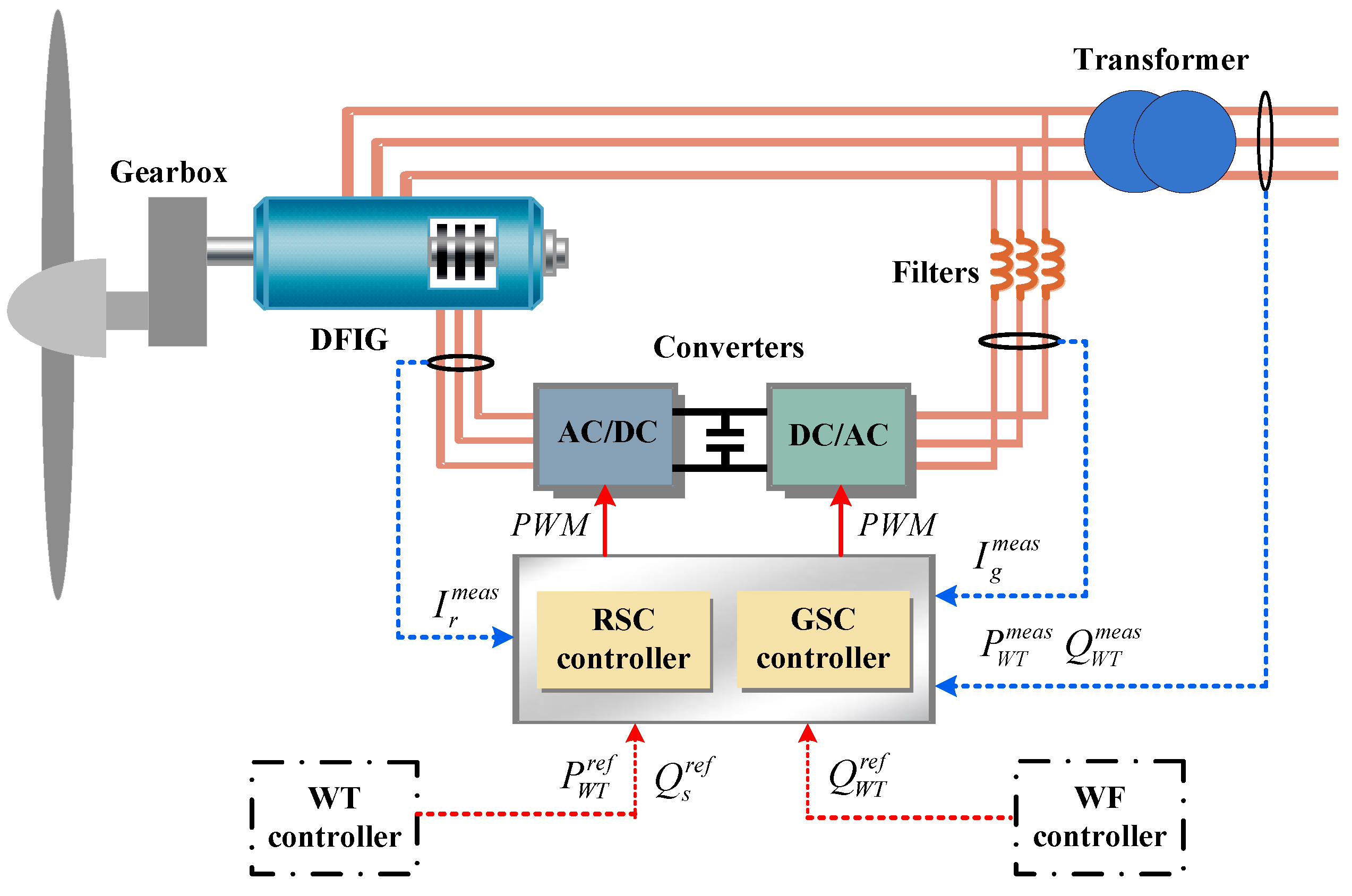
The reactive power control strategies inside a DFIG based WT system are reviewed in this section. The typical control flow of the converters inside a DFIG based WT system is shown in Figure 2.
The total reactive power reference of the WT, , is received from the WF controller, while the reference of reactive power from the stator of the DFIG is set by the WT controller. Therefore, the reactive power reference for GSC can be calculated by:
The total reactive power requirement can be provided by either RSC or GSC, or the combined effort of both RSC and GSC.
3.1. Strategy 1: = 0
This strategy is proposed in [30,31]. The reactive power required by the WF controller is only provided from the stator side. In this case, the reactive power is controlled by the RSC, which also controls the WT active power. In the RSC controller, the q-axis current of the DFIG rotor is controlled to regulate the stator reactive power . This method is commonly used, but it will cause more copper loss inside the DFIG if the required power factor is far from the unity power factor.
3.2. Strategy 2: = 0
In this control concept, the reactive power is only provided by the GSC [30,32]. In this case, GSC is responsible for regulating the reactive power and keeping the dc-link voltage constant, which are controlled by the q-axis current and d-axis current , respectively. This method can fully utilize the capacity of the GSC, but it will increase the losses from the GSC and the filter and the copper loss is not minimal.
3.3. Strategy 3: Minimum Copper Loss Control
The copper loss minimizing strategy is proposed in [33,34]. This method regulates reactive power using both the RSC and the GSC. The reactive power sharing between the RSC and the GSC can be derived using the method described in Equation (11). The optimal reactive current can be derived by equating the derivative of the copper loss with respect to to zero. The result can be expressed as:
Then, the optimal stator side reactive power can be calculated using the steady-state voltage equations of the DFIG in [25]:
Further, the reference reactive power of the GSC can be calculated by Equation (9). This method can minimize the copper losses in the DFIG. However, it may increase the losses from the GSC and the filter, which contributes to a significant part of the total loss.
3.4. Strategy 4: Minimum WT Loss Control
A strategy which shares the reference reactive power of the RSC and the GSC to minimize the total loss is proposed in [35,36]. The sharing ratio is iteratively calculated and a look-up table is formed, which can be used to set the reactive power reference for the GSC controller and the RSC controller. The loss of the filter is included in the objective function in [37] for minimizing the total electrical losses inside the DFIG-based WT system. The authors derived an equation to calculate the reference of the q-axis rotor current with the changing variables and . However, this equation is derived based on the piecewise-linear model of the converter loss, which will cause errors. The proper and of each WT can also be dispatched by the centralized WF controller [25]. However, this will increase the computational burden on the centralized WF controller. In fact, the optimal can be found by solving an optimization problem in Equation (12) under certain and , which is an extension to the method proposed in [35,36].
The constraints for this optimization problem include Equation (9) and the WT reactive power limits.
3.5. Range of Reactive Power
The range of is mainly constrained by the rated rotor side current, which is the rated RSC current and the rated stator current [31]:
The range of is determined by the rated current of the GSC [31]:
These constraints are nonlinear constraints and the currents are calculated using the steady state equations of the system.
4. Reactive Power Dispatch Strategies within a WF
Besides the WT level reactive power control strategy, the WF level reactive power dispatch strategy is critical to the total loss minimization in WFs. This section reviews the reactive power dispatch strategies within a WF.
4.1. Strategy A: Proportional Dispatch
The traditional dispatch strategy is the proportional dispatch, which distributes the reference reactive power required by the WF operator proportionally among all the operational WTs based on their available reactive power [38,39,40,41,42]. This scheme can be expressed using the following equation:
where and are the reference reactive power and the available reactive power of , respectively, and is the WF total reactive power requirement.
This method has the advantage that it can be easily implemented and can ensure that the reactive power reference of each WT does not exceed its limit. However, the active power losses are not considered.
4.2. Strategy B: WF Transmission Loss Minimization
This strategy minimizes the active power losses along the transmission system in a WF, which includes the transmission cables and the transformers for WTs [12,43,44,45,46]. The optimization objective for this strategy is:
where and represent the active power losses for the i-th transformer and the k-th cable, respectively.
This strategy aims at minimizing the active power losses along the transmission system; however, the active power losses inside the WTs are not considered, which are actually responsible for a great share of the total loss.
4.3. Strategy C: WF Total Loss Minimization
This strategy includes the losses along the transmission system, as well as the losses inside the WTs, in the objective [25,47,48]. Thus, the optimization problem can be written as:
s.t.
where and are the active power loss inside the i-th WT and reactive power loss on the k-th cable, respectively; , , and are the active power, reactive power, and voltage at the j-th bus, respectively; and and are the reactive power set point of the i-th WT and the WF, respectively. The calculation of , and uses Equations (1)–(8), which are introduced in Section 2. The voltage range is set as [0.95, 1.05] in all of the case studies.
This strategy considers all of the losses inside the WF in the optimization objective, which is promising for producing the lowest active power loss for the WF.
5. Combinations of WT Level Control and WF Level Dispatch and the Optimization Method
The reactive power control strategies at the WT level can affect the total loss inside the WT under certain and . If the wind distribution and the active power control strategy for each WT are determined, the reactive power dispatch strategy at the WF level will influence not only the transmission losses, but also the losses inside the WTs. Therefore, from the WF controller’s perspective, it is reasonable to find the possible combinations of reactive power control strategies at the WT level and reactive power dispatch strategies at the WF level to check which combination gives the best performance.
5.1. Combinations of WT Level Control and WF Level Dispatch
Based on the aforementioned description, there are twelve reasonable combinations of WT level control and WF level dispatch strategies, which are listed in Table 1.
Many of the combined strategies have been proposed in previous literature. For example, Strategy A1, which is the combination of Strategy A and Strategy 1, has been introduced in [38,39,40,41]. This method is the most common and basic strategy used in WF control.
Strategy C4 is the combination of the WF total loss minimization strategy at WF level and minimum WT loss control at WT level. This strategy has the best chance to reach the minimum active power loss for the WF; however, it may be very difficult to implement because of the complexity. There are different ways to implement Strategy C4. The scheme proposed in [18] uses the centralized WF controller to dispatch the optimal and to each WT, which will change the control strategy of the WT, i.e., each WT should receive two references from the WF controller. Besides, this method doubles the optimization variables, and will thus demand many more computational resources for the WF controller.
In this paper, the optimization problem of Strategy 4 is considered as the inner loop of the optimization problem of Strategy C. The problem is formulated as Equation (12) and is solved offline to generate a lookup table , rather than being solved online. In the process of solving the optimization problem of Strategy C, the optimal is found by searching the lookup table, which saves computational effort for the WF controller.
In order to calculate the currents of the cables and the voltages of each bus, the AC power flow should be implemented. However, it is not easy to include the AC power flow in the optimization problem. In this paper, the AC power flow is computed using the Newton-Raphson method and is considered as an inner loop of the optimization problem. The solutions giving infeasible power flow will be excluded.
5.2. Optimization Method
The problems for WF dispatch strategies B and C are nonlinear and non-convex, and therefore, the PSO algorithm is chosen to provide the solution [49]. In order to improve the performance of standard PSO, a linearly time-varying acceleration constant is applied, as suggested in [49]. It modifies the velocity updating method with a high cognitive constant () and low social constant (), and gradually decreases and increases to search the entire search space, rather than to converge towards a local minimum:
where k is the iteration number and kmax is the maximum iteration number.
A method for improving the convergence speed of the Modified PSO (MPSO) is properly handling the constraints. In this paper, a penalty factor method [50] is adopted to handle the constraints, where the objective function for strategies B and C will be defined by:
where is the total loss of the WF; and are the penalty factors for the equality constraints and inequality constraints, respectively; and ceq and c are the equality constraints and inequality constraints for the optimization problem, respectively, which can be expressed as:
where the tolerance of the voltage violation is selected as 0.05 in this paper, the unit for all the variables in ceq is kW, and all of the variables in c are in per unit system. The penalty factors and are chosen as 0.03 and 100, respectively.
6. Case Study
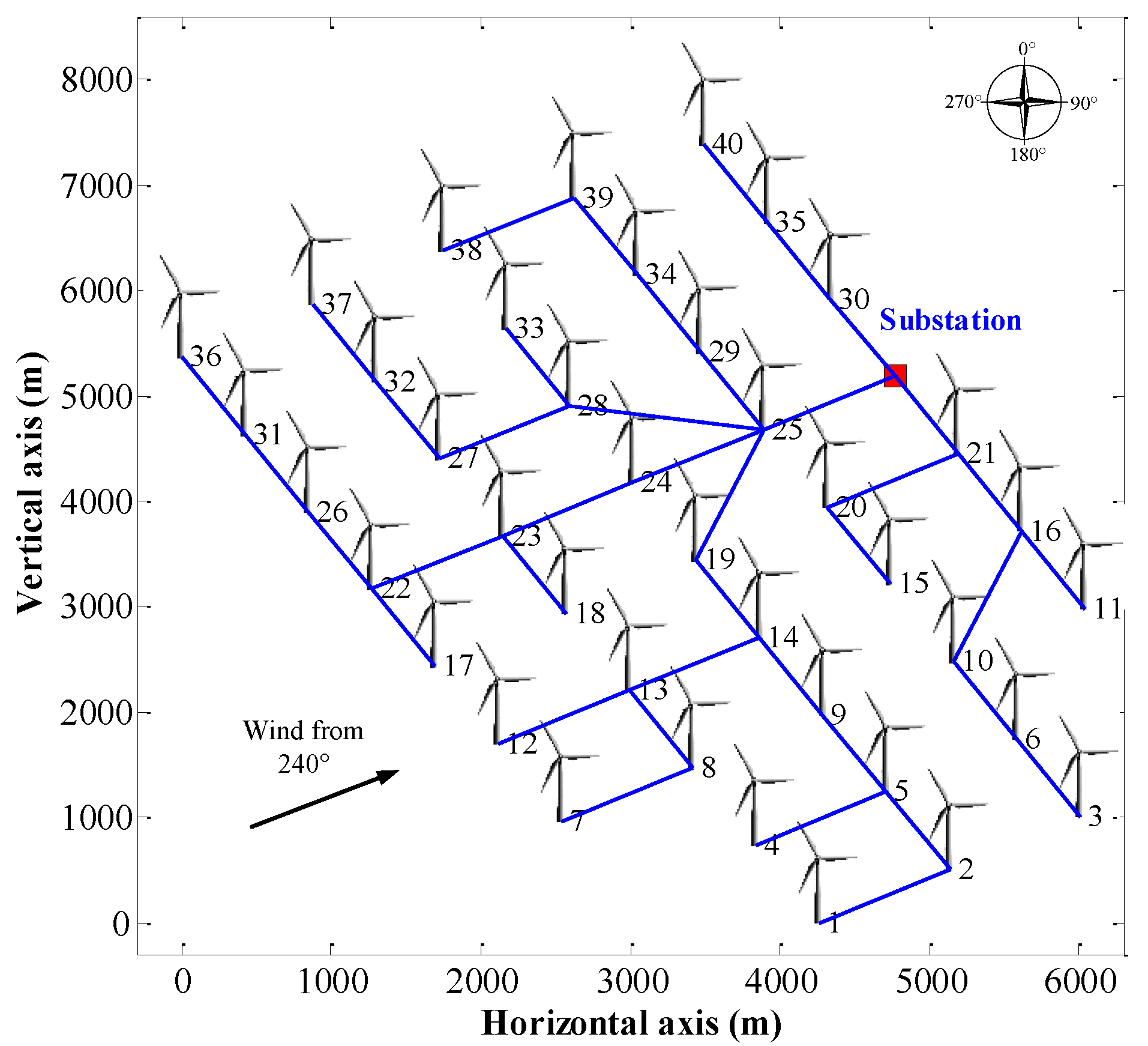
In this paper, a WF with 40 NREL 5MW reference WTs is used to test the combined strategies, as shown in Figure 3. The distance between WTs in the prevailing wind direction is 8 rotor diameters and in the non-prevailing wind direction is 6.7 rotor diameters. The red square is the substation and the number besides the red stars indicates the predefined WTs’ sequence number. The blue line shows the cables connecting the WTs and the substation. The cables are 630, 500, 300, 240, or 95 mm2 (chosen by load) XLPE-Cu cables, which are operated at a 66 kV nominal voltage. The parameters of the WTs are the same as in [25]. The MPSO method is employed to solve the optimization problems.
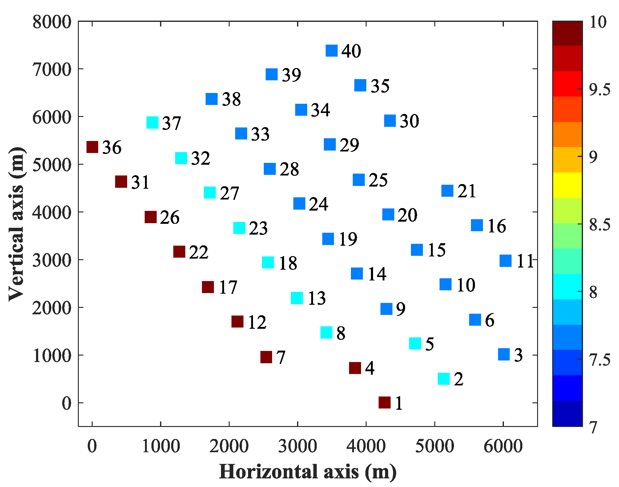
6.1. Case I: V = 10 m/s, Wind Direction = 240°
Considering the wake effect, the wind velocities in front of each WT are different. By using the traditional MPPT control strategy of WTs, the active powers of each WT will be different if the wind velocities are below the rated value. Since the reactive power dispatch between WTs is highly related to their active power, the active power distribution in the WF should be calculated beforehand. In this paper, the wakes are calculated by the Jensen model and the wake combination refers to the multiple wake model in [33]. In this scenario, the wind velocities at each WT are shown in Figure 4.
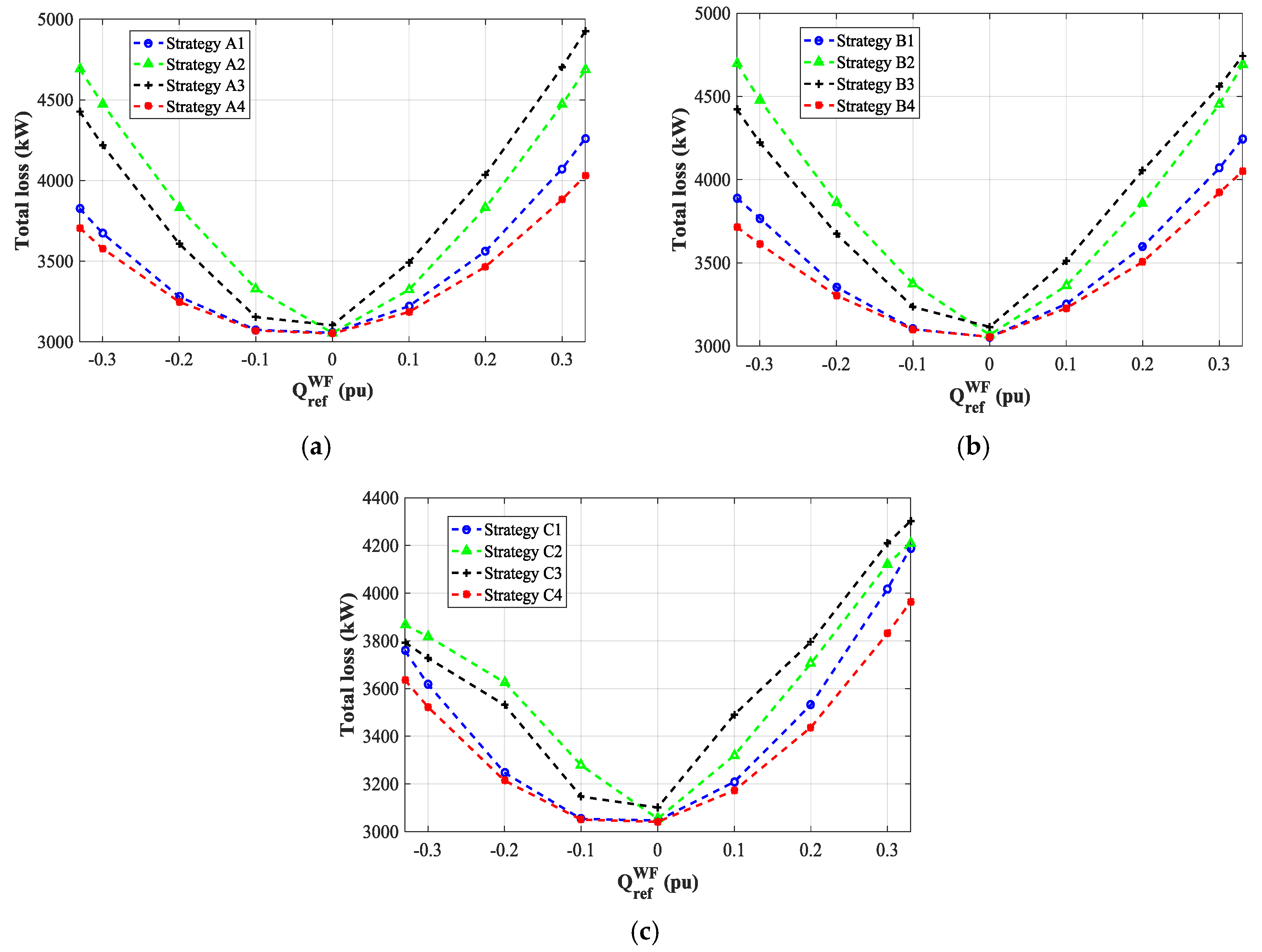
The performances of four WT control strategies with each WF dispatch strategy are shown in Figure 5. As can be seen, the total loss of the WF using WT control Strategy 4 (the red dashed line) is always optimal with all three WF dispatch strategies. Meanwhile, the WT control Strategy 1 (the blue dashed line) is the second best. Using WT control Strategy 4, the total losses are almost the same as when is −0.1 pu and 0 pu. That is because the minimum loss for the DFIG is reached when absorbing a portion of reactive power from the stator side. Therefore, the best for the minimal total loss should lie between 0 pu and −0.1 pu. By the same reason, WT control Strategy 3 (the black dashed line) causes more loss than WT control Strategy 2 (the green dashed line) when is larger than zero.
Since WT control Strategy 4 has the best performance of the four WT control strategies, it is used as the base WT control strategy to compare the performances of the WF dispatch strategies. The results are shown in Figure 6, from which it can be seen that WF dispatch Strategy C exhibits the best performance, while WF dispatch Strategy B causes the largest total loss. Besides, the WF total loss is higher when is positive rather than negative, though the absolute value of is the same. That is also because the loss in the DFIG is minimal when absorbing a portion of reactive power from the stator side.
The losses using Strategies A4, B4 and C4 are shown in Table 2. It can be seen that the losses inside the WTs and the losses on the transformers using Strategy A4 are the minimum. The losses along the cables using Strategy B4 are the minimum; however, the losses inside the WTs and the losses from the transformers using Strategy B4 are the highest, and the total loss using Strategy B4 is the highest. This means that Strategy B4 can minimize the losses in the cables, but increases the losses in the WTs and transformers more significantly. None of the losses on individual parts using Strategy C4 are optimal, but the total loss using Strategy C4 is the minimum, which means the minimal total loss is reached as a compromise of the trend to minimize the losses along the cables and the trend to minimize the losses in the WTs and transformers.
Strategy A is the proportional dispatch of the reactive power. The implementation of Strategy A needs iterations to reduce the error between the actual output reactive power and the reference reactive power at the PCC. Strategies B and C need to solve a nonlinear and nonconvex optimization problem by MPSO, which is quite time consuming compared to the real-time implementation requirement. Therefore, Strategies B and C are solved offline to generate lookup-tables, which are used for online implementation. This method is called the lookup table-based method. The lookup tables are generated offline using a series of wind velocities, wind directions, and reactive power reference of the WF.
The computing times of these strategies are compared in Table 3. The computing time for generating the lookup table result in each scenario and the computing time for real-time implementation were calculated. The swarm size of the MPSO for solving Strategy B and Strategy C is set as 50 and the maximum iteration time setting is 60. In order to obtain better results, the MPSO is repeated 50 times for each scenario and the best result is adopted for generating the lookup tables. An Intel(R) Core(TM) i7-4800MQ [email protected] GHz processor with 8 GB RAM is used for the simulation. The maximum reactive power error at the PCC for Strategy A is set as 0.1 kVA. The offline calculation for Strategies B and C in each scenario is conducted using parallel computing with four cores. In can be seen from Table 3 that though the offline calculation of Strategies B and C is very time consuming, the online implementation of the lookup tables is very fast. Different strategies are suitable for different cases. In the case where the wakes are simulated accurately, the lookup table-based method, Strategy C4, is the best strategy regarding the active power loss. In the case where the wakes simulation may cause large errors, Strategy A4 may be the best strategy regarding the active power loss and online implementation.
6.2. Case II:
In this case, performances of these strategies will be evaluated under different wind directions. The total losses using Strategies A4, B4, and C4 are calculated when is 0.3 pu and the wind direction varies from 180° to 270° at 10° intervals. The results are shown in Figure 7. The total loss in direction 240° is lower than that in other wind directions, because the stronger wake effects in this direction make the wind power at downwind WTs lower, which leads to reduced losses in the WF. However, the loss reduction in this direction is higher than those in other directions. The reason for this is that stronger wake effects cause a higher diverse for the wind distribution in the WF, and thus a higher diverse for the active power distribution. A higher diverse in active power generates more space for reducing the total loss by properly dispatching the reactive power.
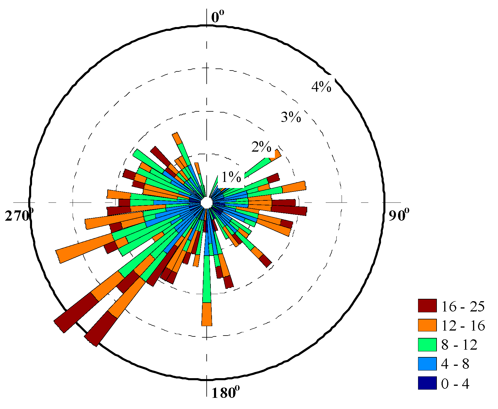
6.3. Case III: Total WF Loss in a Year
In this case, the effectiveness of Strategies A4, B4 and C4 are evaluated in a year. The wind data is obtained from a WF called FINO 3, where the wind speeds are sampled per 3 hours, and then averaged each day. The wind rose is plotted with the intervals of wind directions and wind velocities as 5° and 4 m/s, respectively, as shown in Figure 8.
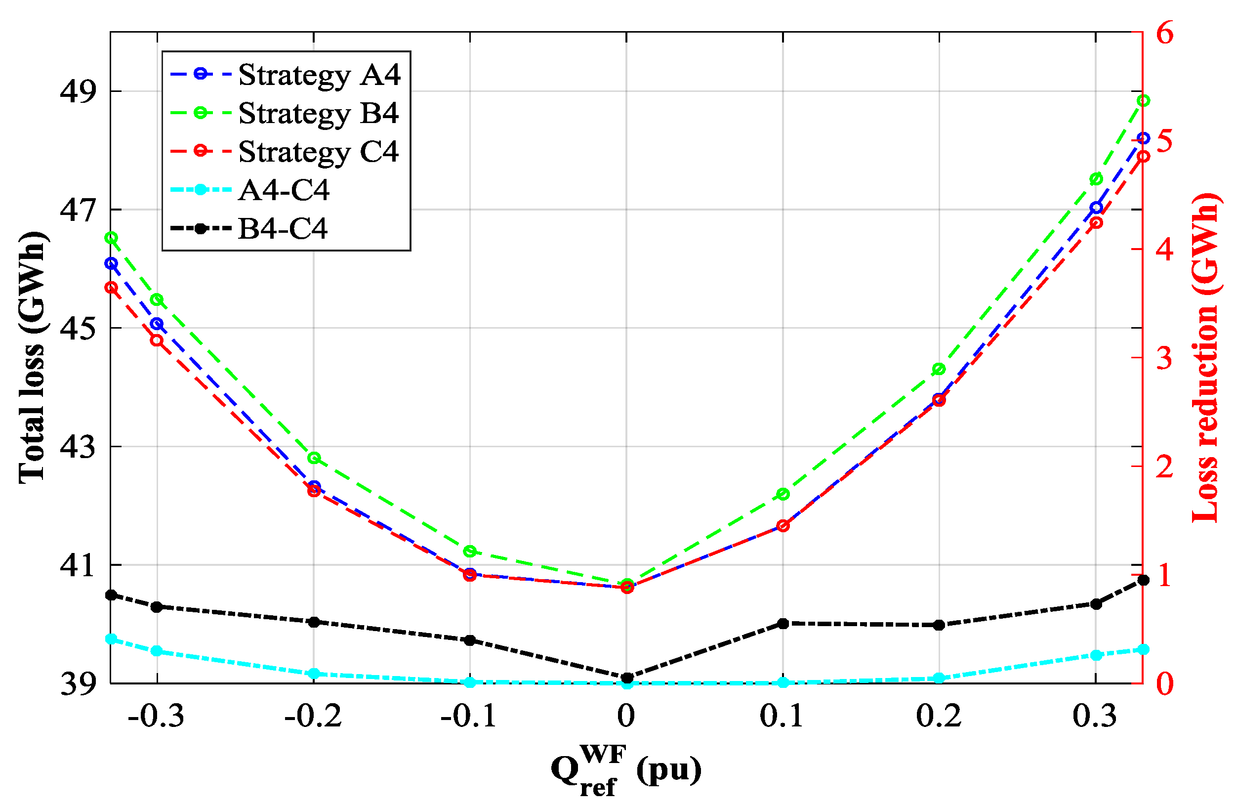
With the data from the wind rose, the total loss using Strategies A4, B4 and C4 are calculated at each wind speed and summed up as the total loss in one year at each , as seen in Figure 9. Compared with Strategy A4, Strategy C4 can save around 0.3 GWh electricity when operating at = 0.33 pu for the whole year. The saving amount of Strategy C4 reaches around 1 GWh when compared with Strategy B4, which is the largest saving amount for every . Based on the results calculated in every case, the WF reactive power dispatch Strategy C4 can ensure minimal active power losses among all of the twelve combined strategies. Meanwhile, Strategy A4 is the second best for loss minimization. However, the implementation of Strategy A4 is much easier than the implementation of Strategy C4, because Strategy C4 needs to solve a nonlinear and nonconvex optimization problem, which requires more computing resources. Therefore, Strategy A4 can be a good choice in WFs with limited computing resources.
7. Conclusions
The total loss in a WF with twelve possible combinations of three WF reactive power dispatch strategies and four WT reactive power control strategies is calculated and compared in different cases. The following conclusions can be drawn based on the results and analysis:
- The reactive power control strategies on the WF level and the WT level interact with each other and should be considered at the same time to achieve a further loss reduction.
- When considering the loss minimization in the WF, the losses of every device, including the losses of the generators, converters, filters, transformers, and cables should be included in the objective at the same time, because reducing the losses on parts of the devices may increase the losses on the other parts.
- The dispatch of reactive power is strongly related to the distribution of the active power. The stronger the wake effect is, the larger the improvement is when using the optimal dispatch strategy.
- The WF losses are lower when is negative, which is because the copper loss on the DFIG is minimal when the stator absorbs a certain amount of inductive reactive power.
- Strategy C4 can give the minimum WF active power loss, but Strategy A4 can be a good choice in WFs with limited computing resources.
The combined strategies can be implemented in the WF energy management system. For future research, different active power dispatch strategies can be combined with the optimal reactive power dispatch strategy.
Acknowledgments
This research work is supported by the Program for Professor of Special Appointment (Eastern Scholar) at the Shanghai Institutions of Higher Learning, and the Danish ForskEL project Harmonized Integration of Gas, District Heating and Electric Systems (HIGHE, 2014-1-12220).
Author Contributions
Baohua Zhang is the main author of this work. This paper provides a further elaboration of some of the results associated with his Ph.D. dissertation. Zhe Chen, Weihao Hu, Jin Tan, and Mohsen Soltani have supported the research in terms of both scientific and technical expertise. Peng Hou contributed to the programming work in the paper. All authors have been involved in the manuscript preparation.
Conflicts of Interest
The authors declare no conflict of interest.
References
- Global Wind Energy Council. Global Wind Report—Annual Market Update. 2015. Available online: http://www.gwec.net/publications/global-wind-report-2/ (accessed on 22 June 2017).
- New Record-Breaking Year for Danish Wind Power. Available online: https://en.energinet.dk/About-our-news/News/2017/04/25/New-record-breaking-year-for-Danish-wind-power (accessed on 22 June 2017).
- Tan, J.; Zhang, Y. Coordinated control strategy of a battery energy storage system to support a wind power plant providing multi-timescale frequency ancillary services. IEEE Trans. Sustain. Energy 2017. [Google Scholar] [CrossRef]
- Technical Regulation 3.2.5 for Wind Power Plants with a Power Output above 11 kW. Available online: https://en.energinet.dk/Electricity/Rules-and-Regulations/Regulations-for-grid-connection (accessed on 22 June 2017).
- National Grid Electricity Transmission plc. The Grid Code—Issue 5, Revision 21. Available online: http://www2.nationalgrid.com/uk/industry-information/electricity-codes/grid-code/the-grid-code/ (accessed on 22 June 2017).
- Zhao, X.; Guerrero, J.M.; Savaghebi, M.; Vasquez, J.C.; Wu, X.; Sun, K. Low-voltage ride-through operation of power converters in grid-interactive microgrids by using negative-sequence droop control. IEEE Trans. Power Electron. 2017, 32, 3128–3142. [Google Scholar] [CrossRef]
- Wang, Y.; Wang, X.; Chen, Z.; Blaabjerg, F. Distributed optimal control of reactive power and voltage in islanded microgrids. IEEE Trans. Ind. Appl. 2017, 53, 340–349. [Google Scholar] [CrossRef]
- Wang, Y.; Chen, Z.; Wang, X.; Tian, Y.; Tan, Y.; Yang, C. An estimator-based distributed voltage-predictive control strategy for AC islanded microgrids. IEEE Trans. Power Electron. 2015, 30, 3934–3951. [Google Scholar] [CrossRef]
- Rueda-Medina, A.C.; Padilha-Feltrin, A. Distributed generators as providers of reactive power support—A market approach. IEEE Trans. Power Syst. 2013, 28, 490–502. [Google Scholar] [CrossRef]
- Ela, E.; Gevorgian, V.; Fleming, P.; Zhang, Y.C.; Singh, M.; Muljadi, E.; Scholbrook, A.; Aho, J.; Pao, L.; Singhvi, V.; et al. Active Power Controls from Wind Power: Bridging the Gaps; Tech. Report: NREL/TP-5D00-605742013; National Renewable Energy Laboratory: Golden, CO, USA, 2014. [Google Scholar]
- Saraswat, A.; Saini, A.; Saxena, A.K. A novel multi-zone reactive power market settlement model: A pareto-optimization approach. Energy 2013, 51, 85–100. [Google Scholar] [CrossRef]
- Sørensen, P.E.; Hansen, A.D.; Iov, F.; Blaabjerg, F.; Donovan, M.H. Wind Farm Models and Control Strategies; Tech. Report: Risø-R-1464(EN); Risø National Laboratory: Roskilde, Denmark, 2005. [Google Scholar]
- Zhao, B.; Li, H.; Wang, M.; Chen, Y.; Liu, S.; Yang, D.; Yang, C.; Hu, Y.; Chen, Z. An optimal reactive power control strategy for a DFIG-based wind farm to damp the sub-synchronous oscillation of a power system. Energies 2014, 7, 3086–3103. [Google Scholar] [CrossRef]
- Hou, P.; Hu, W.; Zhang, B.; Soltani, M.; Chen, C.; Chen, Z. Optimised power dispatch strategy for offshore wind farms. IET Renew. Power Gener. 2016, 10, 399–409. [Google Scholar] [CrossRef]
- Morren, J.; deHaan, S.W.H. Ridethrough of wind turbines with doubly-fed induction generator during a voltage dip. IEEE Trans. Energy Convers. 2005, 20, 435–441. [Google Scholar] [CrossRef]
- Rahimi, M.; Parniani, M. Efficient control scheme of wind turbines with doubly fed induction generators for low-voltage ride-through capability enhancement. IET Renew. Power Gener. 2010, 4, 242. [Google Scholar] [CrossRef]
- Pannell, G.; Zahawi, B.; Atkinson, D.J.; Missailidis, P. Evaluation of the performance of a dc-link brake chopper as a DFIG low-voltage fault-ride-through device. IEEE Trans. Energy Convers. 2013, 28, 535–542. [Google Scholar] [CrossRef]
- Wessels, C.; Gebhardt, F.; Fuchs, F.W. Fault ride-through of a DFIG wind turbine using a dynamic voltage restorer during symmetrical and asymmetrical grid faults. IEEE Trans. Power Electron. 2011, 26, 807–815. [Google Scholar] [CrossRef]
- Zhu, R.; Deng, F.; Chen, Z.; Liserre, M. Enhanced control of DFIG wind turbine based on stator flux decay compensation. IEEE Trans. Energy Convers. 2016, 31, 1366–1376. [Google Scholar] [CrossRef]
- Zhu, R.; Chen, Z.; Wu, X.; Deng, F. Virtual damping flux-based LVRT control for DFIG-based wind turbine. IEEE Trans. Energy Convers. 2015, 30, 714–725. [Google Scholar] [CrossRef]
- Xie, D.; Xu, Z.; Yang, L.; Østergaard, J.; Xue, Y.; Wong, K.P. A comprehensive LVRT control strategy for DFIG wind turbines with enhanced reactive power support. IEEE Trans. Power Syst. 2013, 28, 3302–3310. [Google Scholar] [CrossRef]
- Jensen, N.O. A Note on Wind Generator Interaction; Tech. Report: Risø-M-2411; Risø National Laboratory: Roskilde, Denmark, 1983. [Google Scholar]
- Martinez-Rojas, M.; Sumper, A.; Gomis-Bellmunt, O.; Sudrià-Andreu, A. Reactive power dispatch in wind farms using particle swarm optimization technique and feasible solutions search. Appl. Energy 2011, 88, 4678–4686. [Google Scholar] [CrossRef]
- Krajangpan, K.; Sadara, W.; Neammanee, B. Control strategies for maximum active power and minimum copper loss of doubly fed induction generator in wind turbine system. In Proceedings of the 2010 International Conference on Power System Technology, Hangzhou, China, 24–28 October 2010; pp. 1–7. [Google Scholar]
- Zhang, B.; Hou, P.; Hu, W.; Soltani, M.; Chen, C.; Chen, Z. A reactive power dispatch strategy with loss minimization for a DFIG-based wind farm. IEEE Trans. Sustain. Energy 2016, 7, 914–923. [Google Scholar] [CrossRef]
- Ullah, N.R.; Bhattacharya, K.; Thiringer, T. Wind farms as reactive power ancillary service providers-technical and economic issues. IEEE Trans. Energy Convers. 2009, 24, 661–672. [Google Scholar] [CrossRef]
- Petersson, A. Analysis, Modeling and Control of Doubly-Fed Induction Generators for Wind Turbines. Ph.D. Thesis, Chalmers University of Technology, Göteborg, Sweden, 2005. [Google Scholar]
- Siemens Power Engineering Guide: Transformer. Available online: http://www.energy.siemens.com/hq/pool/hq/power-transmission/Transformers/downloads/peg-kapitel-5.pdf (accessed on 31 October 2016).
- Saadat, H. Power System Analysis; WCB/McGraw-Hill: Boston, MA, USA, 1999. [Google Scholar]
- Kayk, M.; Milanovi, J.V. Reactive power control strategies for DFIG-based plants. IEEE Trans. Energy Convers. 2007, 22, 389–396. [Google Scholar] [CrossRef]
- Zhou, D.; Blaabjerg, F.; Lau, M.; Tonnes, M. Thermal behavior optimization in multi-MW wind power converter by reactive power circulation. IEEE Trans. Ind. Appl. 2014, 50, 433–440. [Google Scholar] [CrossRef]
- Pena, R.; Clare, J.C.; Asher, G.M. Doubly fed induction generator using back-to-back PWM converters and its application to variable-speed wind-energy generation. IEE Proc. Electr. Power Appl. 1996, 143, 231–241. [Google Scholar] [CrossRef]
- Tang, Y.; Xu, L. A flexible active and reactive power control strategy for a variable speed constant frequency generating system. IEEE Trans. Power Electron. 1995, 10, 472–478. [Google Scholar] [CrossRef]
- Abo-Khalil, A.G.; Park, H.-G.; Lee, D.-C. Loss minimization control for doubly-fed induction generators in variable speed wind turbines. In Proceedings of the 33rd Annual Conference of the IEEE Industrial Electronics Society, Taipei, Taiwan, 5–8 November 2007; pp. 1109–1114. [Google Scholar]
- Rabelo, B.; Hofmann, W. Control of an optimized power flow in wind power plants with doubly-fed induction generators. In Proceedings of the IEEE 34th Annual Power Electronics Specialist Conference, Acapulco, Mexico, 15–19 June; pp. 1563–1568.
- Rabelo, B.; Hofmann, W.; Pinheiro, L. Loss reduction methods for doubly-fed induction generator drives for wind turbines. In Proceedings of the International Symposium on Power Electronics, Electrical Drives, Automation and Motion, Taormina, Italy, 23–26 May 2006; pp. 1217–1222. [Google Scholar]
- Zhang, B.; Hu, W.; Chen, Z. Loss minimizing operation of doubly fed induction generator based wind generation systems considering reactive power provision. In Proceedings of the 40th Annual Conference of the IEEE Industrial Electronics Society, Dallas, TX, USA, 29 October–1 November 2014; pp. 2146–2152. [Google Scholar]
- Tapia, A.; Tapia, G.; Ostolaza, J.X. Reactive power control of wind farms for voltage control applications. Renew. Energy 2004, 29, 377–392. [Google Scholar] [CrossRef]
- Saenz, J.R.; Tapia, A.; Tapia, G.; Jurado, F.; Ostolaza, X.; Zubia, I. Reactive power control of a wind farm through different control algorithms. In Proceedings of the 4th IEEE International Conference on Power Electronics and Drive Systems, Denpasar, Indonesia, 25–25 October 2001; pp. 203–207. [Google Scholar]
- Tapia, A.; Tapia, G.; Ostolaza, J.X.; Saenz, J.R.; Criado, R.; Berasategui, J.L. Reactive power control of a wind farm made up with doubly fed induction generators II. In Proceedings of the 2001 IEEE Porto Power Tech Proceedings, Porto, Portugal, 10–13 September 2001; pp. 5–9. [Google Scholar]
- Merahi, F.; Berkouk, E.M.; Mekhilef, S. New management structure of active and reactive power of a large wind farm based on multilevel converter. Renew. Energy 2014, 8, 814–828. [Google Scholar] [CrossRef]
- Ghennam, T.; Aliouane, K.; Akel, F.; Francois, B.; Berkouk, E.M. Advanced control system of DFIG based wind generators for reactive power production and integration in a wind farm dispatching. Energy Convers. Manag. 2015, 105, 240–250. [Google Scholar] [CrossRef]
- De Almeida, R.G.; Castronuovo, E.D.; PecasLopes, J.A. Optimum generation control in wind parks when carrying out system operator requests. IEEE Trans. Power Syst. 2006, 21, 718–725. [Google Scholar] [CrossRef]
- Kanna, B.; Singh, S.N. Towards reactive power dispatch within a wind farm using hybrid PSO. Int. J. Electr. Power Energy Syst. 2015, 69, 232–240. [Google Scholar] [CrossRef]
- Zhao, J.; Li, X.; Hao, J.; Lu, J. Reactive power control of wind farm made up with doubly fed induction generators in distribution system. Electr. Power Syst. Res. 2010, 80, 698–706. [Google Scholar] [CrossRef]
- Moyano, C.F.; Peças Lopes, J.A. An optimization approach for wind turbine commitment and dispatch in a wind park. Electr. Power Syst. Res. 2009, 79, 71–79. [Google Scholar] [CrossRef]
- Zhang, B.; Hu, W.; Hou, P.; Chen, Z. Reactive power dispatch for loss minimization of a doubly fed induction generator based wind farm. In Proceedings of the 17th International Conference on Electrical Machines and Systems, Hangzhou, China, 22–25 October 2014; pp. 1373–1378. [Google Scholar]
- Zhang, J.H.; Liu, Y.Q.; Tian, D.; Yan, J. Optimal power dispatch in wind farm based on reduced blade damage and generator losses. Renew. Sustain. Energy Rev. 2015, 44, 64–77. [Google Scholar] [CrossRef]
- Suganthan, P.N. Particle swarm optimiser with neighbourhood operator. In Proceedings of the 1999 Congress on Evolutionary Computation-CEC99, Washington, DC, USA, 6–9 July 1999; pp. 1958–1962. [Google Scholar]
- Clerc, M.; Kennedy, J. The particle swarm—Explosion, stability, and convergence in a multidimensional complex space. IEEE Trans. Evol. Comput. 2002, 6, 58–73. [Google Scholar] [CrossRef]
Figure 1.
Active power losses inside a DFIG based WT.
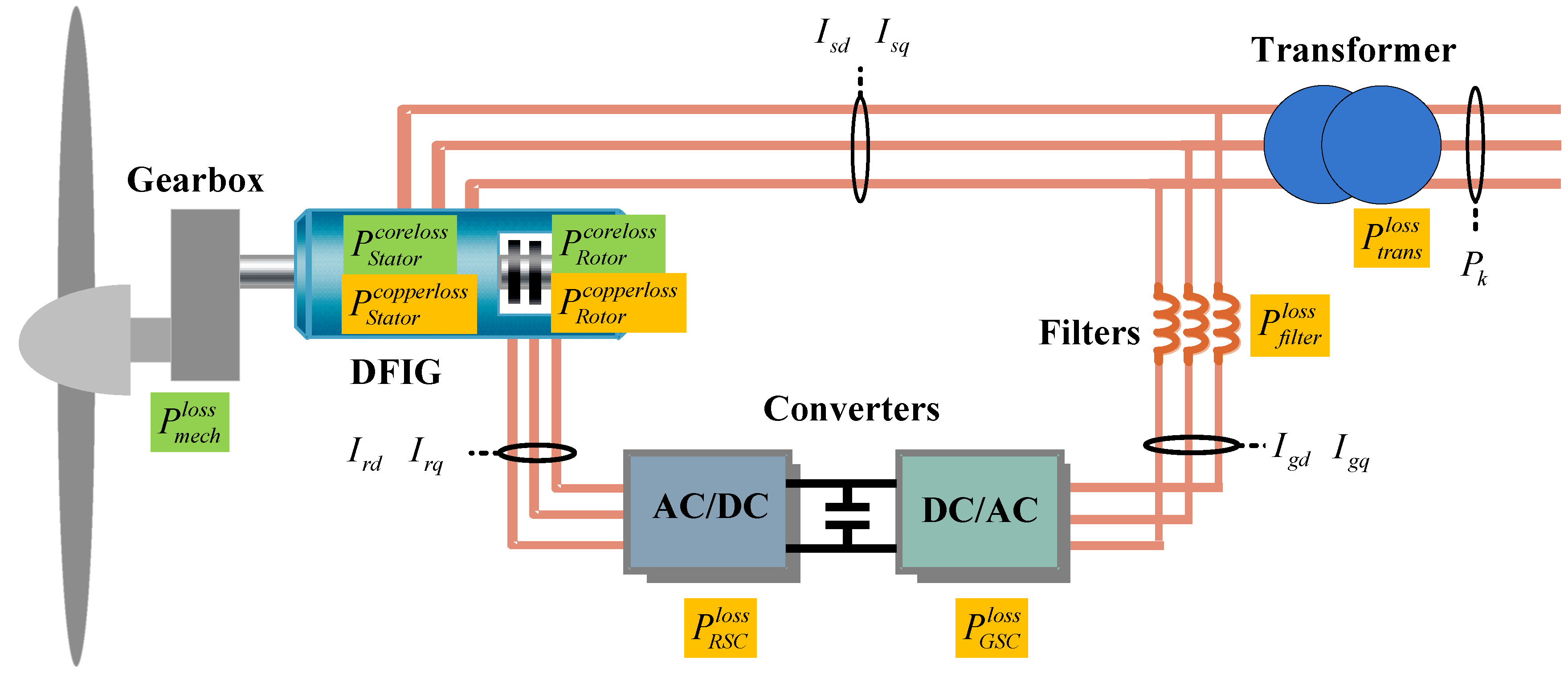
Figure 2.
Typical control flow of a DFIG based WT.

Figure 3.
The WF layout and cable connection.

Figure 4.
The wind velocity at each WT (Unit: m/s).

Figure 5.
The WFs total loss using each WT level control strategy with different WF level dispatch strategies: (a) With WF level dispatch Strategy A; (b) With WF level dispatch Strategy B; (c) With WF level dispatch Strategy C.
Figure 5.
The WFs total loss using each WT level control strategy with different WF level dispatch strategies: (a) With WF level dispatch Strategy A; (b) With WF level dispatch Strategy B; (c) With WF level dispatch Strategy C.

Figure 6.
The WF total loss using each WF dispatch strategy with WT control Strategy 4.
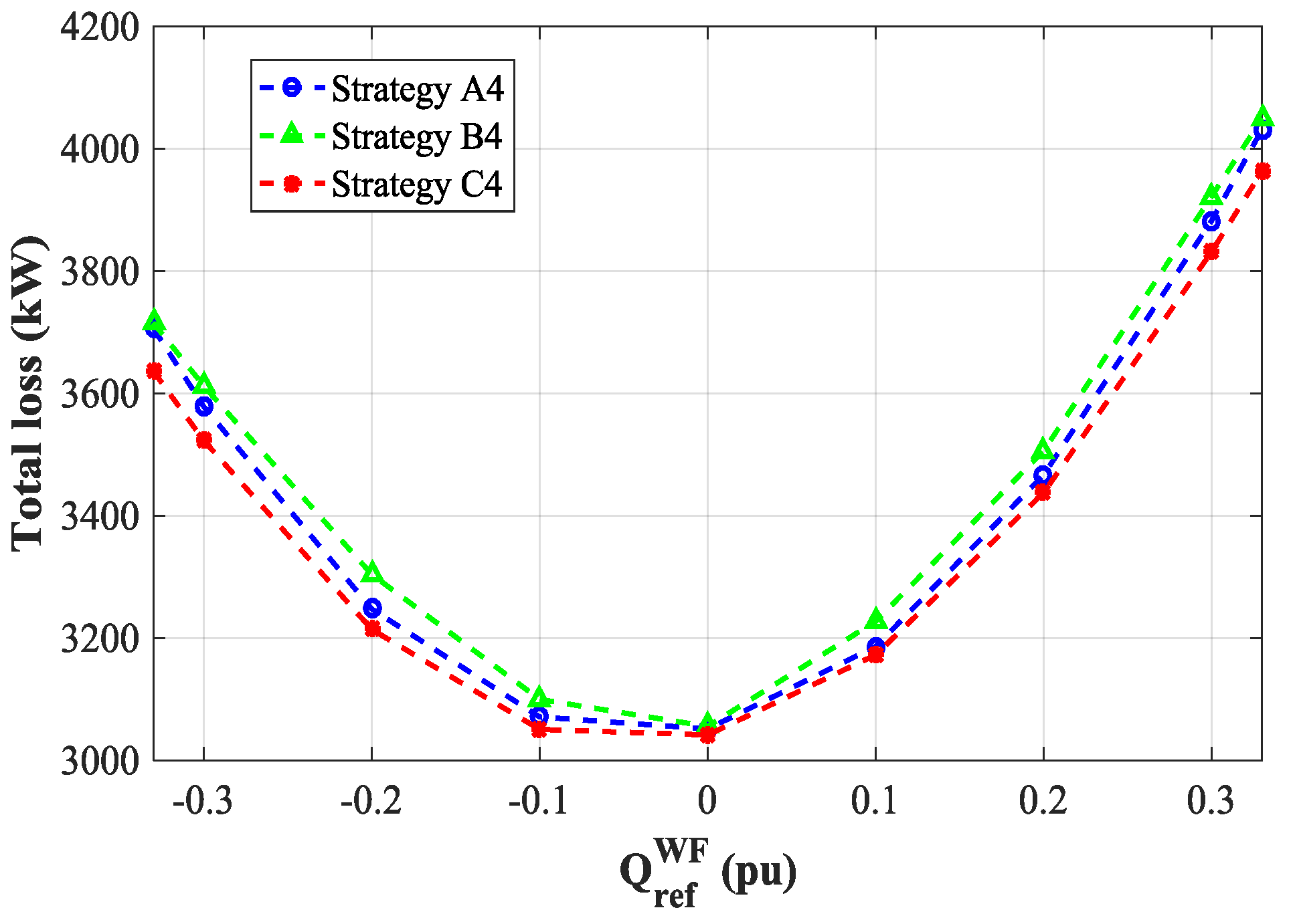
Figure 7.
The total loss using Strategies A4, B4 and C4 and the loss reduction with respect to Strategy C4.
Figure 7.
The total loss using Strategies A4, B4 and C4 and the loss reduction with respect to Strategy C4.
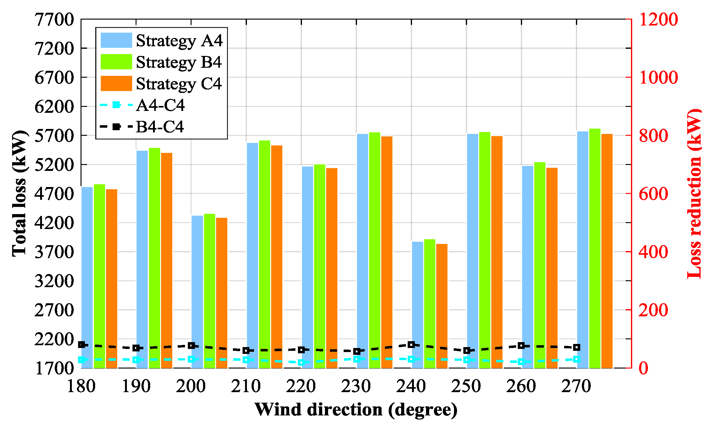
Figure 8.
Wind rose according to the data from the WF: FINO 3.

Figure 9.
Total loss over a year using Strategies A4, B4 and C4.

Table 1.
Combinations of WF level dispatch strategies and WT level control strategies.
| WF Level Dispatch | WT Level Control | Combined Strategy |
|---|---|---|
| Strategy A | Strategy 1 | Strategy A1 [38,39,40,41] |
| Strategy 2 | Strategy A2 [42] | |
| Strategy 3 | Strategy A3 | |
| Strategy 4 | Strategy A4 | |
| Strategy B | Strategy 1 | Strategy B1 [43,44,45,46] |
| Strategy 2 | Strategy B2 | |
| Strategy 3 | Strategy B3 [48] | |
| Strategy 4 | Strategy B4 | |
| Strategy C | Strategy 1 | Strategy C1 [47] |
| Strategy 2 | Strategy C2 | |
| Strategy 3 | Strategy C3 | |
| Strategy 4 | Strategy C4 [25] |
Table 2.
Losses inside the WF using Strategy A4, B4 and C4.
| (pu) | −0.33 | −0.3 | −0.2 | −0.1 | 0 | 0.1 | 0.2 | 0.3 | 0.33 | |
|---|---|---|---|---|---|---|---|---|---|---|
| Loss (kW) | ||||||||||
| A4 | Turbine | 2317 | 2236 | 2028 | 1927 | 1935 | 2050 | 2266 | 2570 | 2677 |
| Transformer | 718 | 708 | 679 | 662 | 656 | 661 | 677 | 704 | 714 | |
| Cable | 671 | 635 | 540 | 482 | 460 | 474 | 524 | 608 | 639 | |
| Total | 3706 | 3579 | 3247 | 3071 | 3051 | 3185 | 3467 | 3882 | 4030 | |
| B4 | Turbine | 2373 | 2315 | 2090 | 1962 | 1939 | 2089 | 2318 | 2645 | 2736 |
| Transformer | 725 | 717 | 688 | 666 | 656 | 661 | 683 | 713 | 722 | |
| Cable | 617 | 580 | 506 | 472 | 460 | 471 | 505 | 563 | 592 | |
| Total | 3715 | 3612 | 3284 | 3100 | 3055 | 3221 | 3506 | 3921 | 4050 | |
| C4 | Turbine | 2319 | 2237 | 2029 | 1927 | 1935 | 2051 | 2267 | 2572 | 2679 |
| Transformer | 719 | 709 | 680 | 662 | 656 | 662 | 678 | 705 | 715 | |
| Cable | 637 | 611 | 533 | 481 | 460 | 473 | 520 | 585 | 612 | |
| Total | 3676 | 3557 | 3241 | 3070 | 3051 | 3186 | 3464 | 3862 | 4006 |
Table 3.
Comparison of the computing time in each scenario using different strategies.
| Strategy | Computing Time for Offline Calculation Using Parallel Computing | Computing Time for Online Implementation |
|---|---|---|
| A1 | - | 0.3 s |
| A2 | - | 0.3 s |
| A3 | - | 0.36 s |
| A4 | - | 0.55 s |
| B1 | 847 s | 0.1 s |
| B2 | 836 s | 0.1 s |
| B3 | 867 s | 0.1 s |
| B4 | 1761 s | 0.1 s |
| C1 | 892 s | 0.1 s |
| C2 | 931 s | 0.1 s |
| C3 | 897 s | 0.1 s |
| C4 | 2011 s | 0.1 s |
© 2017 by the authors. Licensee MDPI, Basel, Switzerland. This article is an open access article distributed under the terms and conditions of the Creative Commons Attribution (CC BY) license (http://creativecommons.org/licenses/by/4.0/).
Share and Cite
MDPI and ACS Style
Zhang, B.; Hu, W.; Hou, P.; Tan, J.; Soltani, M.; Chen, Z. Review of Reactive Power Dispatch Strategies for Loss Minimization in a DFIG-based Wind Farm. Energies 2017, 10, 856. https://doi.org/10.3390/en10070856
AMA Style
Zhang B, Hu W, Hou P, Tan J, Soltani M, Chen Z. Review of Reactive Power Dispatch Strategies for Loss Minimization in a DFIG-based Wind Farm. Energies. 2017; 10(7):856. https://doi.org/10.3390/en10070856
Chicago/Turabian StyleZhang, Baohua, Weihao Hu, Peng Hou, Jin Tan, Mohsen Soltani, and Zhe Chen. 2017. "Review of Reactive Power Dispatch Strategies for Loss Minimization in a DFIG-based Wind Farm" Energies 10, no. 7: 856. https://doi.org/10.3390/en10070856
Note that from the first issue of 2016, this journal uses article numbers instead of page numbers. See further details here.