
Energy-Related CO2 Emissions Forecasting Using an Improved LSSVM Model Optimized by Whale Optimization Algorithm

School of Economics and Management, North China Electric Power University, Beijing 102206, China
*
Author to whom correspondence should be addressed.
Energies 2017, 10(7), 874; https://doi.org/10.3390/en10070874
Submission received: 31 May 2017
/
Revised: 12 June 2017
/
Accepted: 26 June 2017
/
Published: 29 June 2017
Abstract
:Accurate and reliable forecasting on energy-related carbon dioxide (CO2) emissions is of great significance for climate policy decision making and energy planning. Due to the complicated nonlinear relationships of CO2 emissions with its driving forces, the accurate forecasting for CO2 emissions is a tedious work, which is an important issue worth studying. In this study, a novel CO2 emissions prediction method is proposed which employs the latest nature-enlightened optimization method, named the Whale optimization algorithm (WOA), to search the optimized values of two parameters of LSSVM (least squares support vector machine), namely the WOA-LSSVM model. Meanwhile, the driving forces of CO2 emissions including GDP (gross domestic product), energy consumption and population are chosen to be the import variables of the proposed WOA-LSSVM method. Taking China’s CO2 emissions as an instance, the effectiveness of WOA-LSSVM-based CO2 emissions forecasting is verified. The comparative analysis results indicate that the WOA-LSSVM model is significantly superior to other selected models, namely FOA (fruit fly optimization algorithm)-LSSVM, LSSVM, and OLS (ordinary least square) models in terms of CO2 emissions forecasting. The proposed WOA-LSSVM model has the potential to effectively improve the accuracy of CO2 emissions forecasting. Meanwhile, as a new nature-enlightened heuristic optimization algorithm, the WOA has the prospect for wide application.
1. Introduction
With the high speed expansion of globalization and industrialization, energy consumption of the whole world has experienced a rapid increase in the last 2 decades. The consumption of fossil fuel, contributing to economic development to a large extent, constitutes 80% of the global energy consumption [1]. It has become widely that greenhouse gases emissions, particularly CO2 emissions, have destructive impacts on the environment, especially in terms of global warming, primarily from such sources as fossil fuel burning for electricity production and heat supply [2]. In the past 20 years, nearly 75% of the human-caused carbon emissions originated from fossil fuel burning. The scientific opinion holds that CO2 emissions are the main driving forces of climate change [3]. Therefore, it is essential to forecast CO2 emissions from the angle of energy consumption for climate policy making and energy planning. First, CO2 emissions forecasting can not only help predict how future global temperatures will rise, but also help to evaluate prospective expenses of emission reduction, as well as potential benefits from guarding against global temperatures rising [4]. Second, the Copenhagen Accord established that global temperatures rising ought to be confined to below 2 °C, which demands 40–70% emissions decrease by 2050, as compared to emissions in 2010. With the approaching of 2050, various carbon capture technologies have been developed for CO2 emissions reduction to achieve a 2 °C limitation on global warming [5,6,7,8,9]. In addition to carbon capture technologies, CO2 emissions prediction can also contribute toward examining whether the sustained reinforcing of global climate policy has the capability to bring a notable CO2 emissions decrease to achieve the 2 °C goal. If not, the governments need to carry out more aggressive climate policies.
Several kinds of estimation methods have been developed in CO2 forecasting modeling in recent years. The structure model, a popular approach, has been employed in some literatures to forecast CO2 emissions, such as the national energy modeling system (NEMS) and computable general equilibrium (CGE) models [10,11,12]. Nevertheless, these approaches are unable to reflect the dynamic instinct of the real economy, due to the stationary of parameter values in structural models. Therefore, there are also other methods used to forecast CO2 emissions. Meng [13] employed a logistic function to imitate emissions generated from non-renewable energy burning. Liang [14] constructed an input–output model of energy consumption and CO2 emissions of multi-areas in China and carried out scenario analysis for 2010 and 2020. Chen put forward a blended fuzzy regression and back propagation network method, which was used to forecast global CO2 concentration [15]. Pao [16] and Lin [17] employed grey model to forecast CO2 emissions of Brazil and Taiwan. Through estimating China’s future energy demand, He [18] predicted CO2 emissions during the period of 2010 to 2020 on the basis of scenario analysis method. From the previous studies, it can be seen that there are few studies employing the intelligent forecasting techniques (algorithms), which usually have the advantages of strong learning ability and high forecasting accuracy. Therefore, this paper attempts to employ the LSSVM (least squares support vector machine) technique, a famous and widely applied intelligent algorithm, to forecast CO2 emissions.
The LSSVM model has been widely utilized to deal with forecasting issues in different fields, such as gas [19], short-term electric load [20], wind speed [21], and hydropower consumption [22]. However, it is rare to find that the LSSVM technique has been used for CO2 emissions forecasting. Therefore, the application feasibility of LSSVM model to forecast CO2 emissions is examined in this paper. Generally speaking, the LSSVM method relies on the values of two parameters, namely the bandwidth of RBF kernel “” and the regularization parameter “c”. At present, some optimization methods were utilized to find the optimized values for the two parameters, such as genetic algorithm [20], artificial bee colony algorithm [23], chaotic differential evolution approach [24], and FOA (fruit fly optimization algorithm) [25]. However, most of these optimization methods have some disadvantages of being hard to understand, or achieving local optimum but reaching global optimum slowly. The WOA (Whale optimization algorithm), put forward by Seyedali Mirjalili in 2016, is a novel heuristic optimization algorithm enlightened by nature [26]. This new optimization method can be easily understood and achieve the global optimal solution in a quite short time. Considering these superiorities, this study tries to employ the WOA method to optimize two significant parameters of the LSSVM method, with the aim of improving the forecasting performance of CO2 emissions. Simultaneously, at the aim of further improving the prediction accuracy, the main driving factors of CO2 emissions including GDP (gross domestic product), energy consumption and population, are also taken to be the import variables for the established WOA-LSSVM approach to forecast CO2 emissions.
The primary contributions of this paper are the following:
- A novel LSSVM-based CO2 emissions forecasting model is proposed, of which the significant parameters in LSSVM are optimized by the meta-heuristic optimization algorithm WOA. It is verified that this hybrid intelligence forecasting method has the superiority in the forecasting precision of CO2 emissions through comparing with LSSVM model optimized by FOA, LSSVM without parameters optimization and OLS (ordinary least square). This paper extends the application domains of intelligence LSSVM forecasting technique.
- GDP, energy consumption and population, which are considered as the main driving forces of CO2 emissions, are imported into the proposed WOA-LSSVM approach. Therefore, the proposed CO2 emissions prediction model in this paper not only employs the intelligence forecasting technique, but also takes the social economic driving factors of CO2 emissions into consideration, which encapsulates the complicated nonlinear relationships of CO2 emissions with its main driving forces to some extent.
The remainder of the study is processed below. Section 2 represents the theory of WOA method and LSSVM model, and a novel CO2 emissions prediction method (namely WOA-LSSVM) that combines the WOA and LSSVM technique is illustrated. Section 3 proceeds with the empirical simulation and analysis for WOA-LSSVM-based CO2 emissions. In Section 4, the CO2 emissions forecasting performance of different models are compared. Finally, the conclusions are presented in Section 5.
2. The Methodology of WOA-LSSVM Forecasting Model
2.1. Basic Methodology of LSSVM Model
LSSVM is an improvement of the support vector machine (SVM), which replaces the inequality constraints of traditional SVM with equality constraints, studying with the principle of structural risk minimization through employing linear least squares guide lines to the loss function. So, the speed of problem solving and the accuracy of convergence can be enhanced [27]. The fundamental theory of LSSVM method is introduced as below.
Set a series of samples , taking as the entering vector and as the homologous output value of sample . Through employing a nonlinear function , the sample data are mapped to a higher dimension from the customary feature space, therefore, to approximately describe it in a linear form:
where implies the weight vector, and indicates the error.
In the original space, the LSSVM with the equality constraints is expressed as:
where indicates the regularization parameter, and represents the slack variable.
Then, the Lagrangian function L can be established as:
where implies Lagrange multiplier.
The conditions of Karush–Kuhn–Tucker (KKT) for optimal performance are provided by:
Removing the variables and , the majorization issue is converted into the linear form as follows:
where , ; . In accordance with the Mercer’s condition, the Kernel function is described as:
The LSSVM method for regression can be set by:
Owing to a fewer parameters to be set and a superior performance, the radial basis function (RBF) is chosen to be the Mercer kernel function in this paper, which is shown in Equation (8).
Consequently, two parameters are needed to be found if the LSSVM model is utilized to forecast CO2 emissions, which are the bandwidth of RBF kernel “” and the regularization parameter “c”. The latest intelligent algorithm WOA will be applied to search the optimal values of “” and “c”, and the optimization details are introduced in Section 2.2 and Section 2.3.
2.2. Basic Theory of WOA
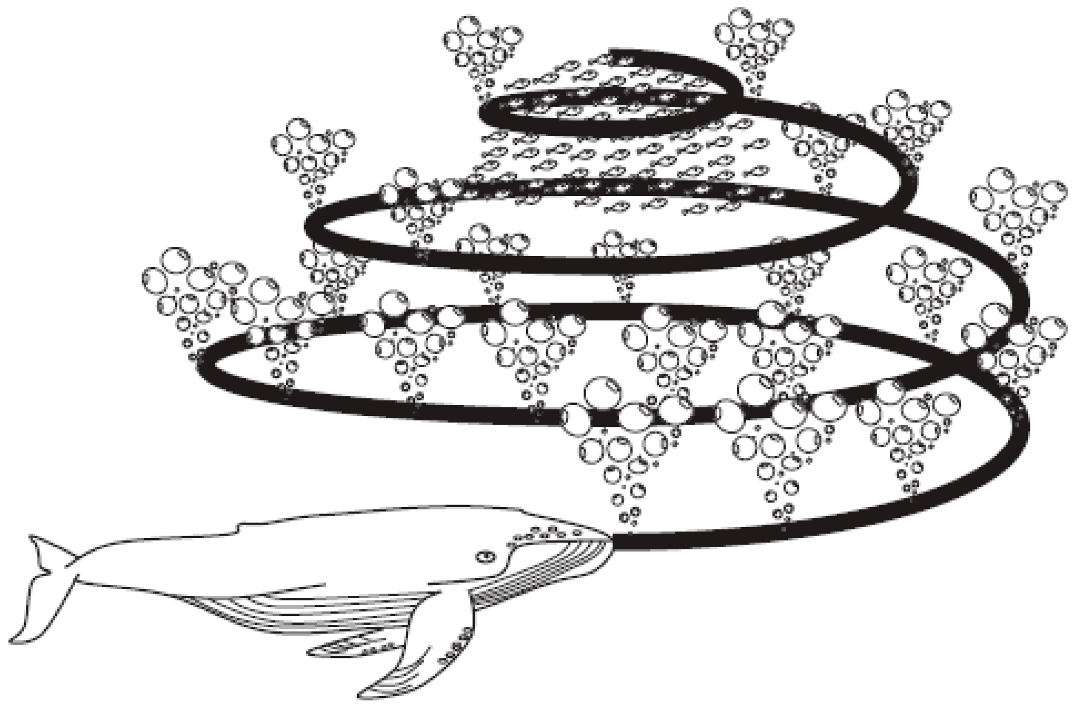
Enlightened by the humpback whales’ special hunting strategy, named the bubble-net feeding method [28], the researcher Seyedali Mirjalili proposed a novel nature-enlightened heuristic optimization method, namely WOA, simulating the public behavior of humpback whales [26]. The foraging behavior investigated by Goldbogen et al. employing tag sensors has found that there are two tactics bound up with the bubble, which are called “upward-spirals” and “double-loops” [29]. In “upward-spirals” strategy, humpback whales dive about 12 m and begin to generate bubbles in a heliciform around the prey and swim up to the surface, which is shown in Figure 1, taken from the original in study [26]. Therefore, it is worth mathematically imitating the heliciform bubble-net predation strategy to carry out optimization. WOA is proposed in accordance with this behavior.
For a detailed description of WOA, please refer to the work documented in study [26]. In accordance with the upward spiral bubble-net foraging maneuver, the WOA method is made up of several steps, which are illustrated as follows:
• Step 1: Parameters setting.
The vital parameters of WOA contain: the amount of search agents SearchAgents_no; the amount of variables dim; the maximum amount of generations Max_iteration; the lower bound , and upper bound of variables.
• Step 2: Population initialization.
As a method on the basis of population, the humpback whales in WOA method can be expressed in a matrix as below:
where W represents the position matrix of humpback whales; means the value of j-th parameter of the i-th humpback whale, , can be calculated by employing stochastic distribution which is indicated in Equation (10).
where is the value of the i-th row, j-th column of the matrix; and imply the lower bound and upper bound of i-th humpback whale; represents the stochastic number generated from uniform distribution in [0, 1] interval.
• Step 3: Fitness function determination.
At the aim of evaluating each humpback whale, the fitness function ought to be determined during the process of majorization, and the matrix is utilized to store the fitness values of humpback whales as follows:
• Step 4: Iteration process.
In WOA method, the search agents renovate their places according to a stochastically selected search agent or the best scheme attained till now. At the aim of performing a global search and avoiding local optimum, the WOA method begins with a series of random solutions, which means the location of a search agent would be updated with regard to a stochastically selected search agent. The mathematical model can be estimated as below:
where t represents the current iteration, and mean coefficient vectors, represents a stochastic location vector (a stochastic humpback whale) selected from the present population, implies the location vector, stands for the absolute value, and indicates an element-be-element multiplication. The vectors and can be computed as below:
where is linearly reduced from 2 to 0 through the process of iterations, and represents a stochastic vector in .
Since the value of depends on the diversification of , a stochastic search agent is selected when , while the best scheme is chosen when to renovate the location of the search agents. Under the condition of , the humpback whales swim around the prey in two forms of paths, which are the shrinking circle and heliciform path.
For the shrinking encircling path, the search agents can renew their positions on the basis of the following equations:
where indicates the location vector of the best solution attained till now. The vectors and can be calculated in accordance with Equations (14) and (15). Through reducing the value of in Equation (14), the shrinking encircling mechanism can be achieved.
For the spiral shaped path, the helix-shaped movement between the humpback whales and prey can be simulated as follows:
where implies the distance of the i-th humpback whale to the prey (best scheme attained till now), means a constant used to determine the shape of the logarithmic spiral, indicates a stochastic number in the interval , and illustrates an element multiplication.
Since the humpback whales swim around the best solution within a shrinking circle path and along a heliciform path at the same time, for the purpose of modeling this simultaneous behavior, it is assumed that there is a 50% probability of selecting either the spiral model or the shrinking circle mechanism to renovate the positions of humpback whales in the majorization process. The mathematical equation can be established as below:
where p represents a stochastic number in interval .
• Step 5: Optimal selection.
During every iteration process, the search agents renovate their places with regard to a stochastically selected search agent or the best scheme attained till now. A stochastic search agent is selected under the condition of and the search agents renew their locations in accordance with the Equation (13), while the best solution is chosen if and the search agents renovate their places according to Equations (17) and (18) relying on the value of p. Finally, the WOA method comes to the termination if the iteration criterion is satisfied.
The primary steps of WOA method are demonstrated in Figure 2.
2.3. Basic Principle of WOA-LSSVM Model for CO2 Emissions Forecasting
It is necessary to determine the optimal values of two parameters for LSSVM method before the operation of CO2 emissions prediction. For the purpose of improving the forecasting performance, the WOA method is utilized to optimize the value of these two parameters.
The process of WOA-LSSVM model for CO2 emissions forecasting is elaborated on below:
• Step 1: Parameters setting.
There are five primary parameters of WOA needed to be set, including the number of whales SearchAgents_no, the number of variables dim, the maximum number of iteration Max_iteration, the lower bound , and upper bound . In this paper, set SearchAgents_no = 50, dim = 2, Max_iteration = 100, , and .
• Step 2: Population initialization.
Since the values of SearchAgents_no, dim, Max_iteration, the lower bound and the upper bound have been initialized, the first stochastic population (location) of whales can be calculated using Equation (10). And the value of iteration is 1 at the original stage.
• Step 3: Fitness function determination.
In this study, the positions of whales are used to represent two parameters of LSSVM model, namely , and . Therefore, and are fed into the LSSVM model for CO2 emissions prediction. In accordance with the CO2 emissions prediction result, the homologous value of fitness function can be computed based on the root mean square error (RMSE) shown in Equation (20) utilized to establish the fitness function in this paper.
where indicates the actual value of CO2 emissions at time ; implies the forecasting value of CO2 emissions at time .
• Step 4: Optimization begins.
At the original iteration (iteration = 1), the fitness values of all the whales are computed based on Equation (20). Then, rank the first population of whales according to their fitness values, and choose the whale with the optimal fitness value. After the best whale is identified, other whales will attempt to renew their places with respect to the best whale, according to Equation (19).
• Step 5: Optimization ends.
When the first iteration comes to the termination, the best whale and the best fitness value of the whale can be obtained. Then, we can begin to generate the offspring generation, and renovate the location and fitness of the whale at each iteration on the basis of Equations (9)–(19). The whales update their positions with regard to the best whales selected according to the fitness value. The best whale and their corresponding fitness value can be obtained after each iteration. Therefore, after 100 iterations, the optimization process comes to the end, and the best position of whale can be obtained. Simultaneously, the regularization parameter “c” and the bandwidth of RBF kernel “” of LSSVM method are attained.
The optimization process of WOA-LSSVM method for CO2 emissions prediction is illustrated in Figure 3.
3. Empirical Simulation and Analysis
3.1. Data Sources and Preprocessing of Data Sample
In this study, the WOA-LSSVM method is utilized to predict the CO2 emissions in China. Before forecasting CO2 emissions, it is critical to determine the key drivers of China’s increasing CO2 emissions, which should be considered as the input variables of the proposed WOA-LSSVM-based CO2 emissions forecasting model. The CO2 emissions and its driving forces show complicated nonlinear relationships. In summarizing previous studies [30,31,32], GDP, population, total exports, energy consumption, and economic structure are found to be the main drivers of CO2 emissions. Based on these findings, we further explore the correlation degrees between these driving forces and China’s CO2 emissions between 1991 and 2014 by using the grey correlation analysis method, which measures the correlation degree between different factors according to the similarity or difference degree of trends, and the values are listed in Table 1. From Table 1, we can infer that GDP, energy consumption and population maintains the top three highest correlation degrees with China’s CO2 emissions, which are 0.6577, 0.6727, and 0.6798, respectively. Therefore, GDP, energy consumption and population are selected as the input variables for WOA-LSSVM-based CO2 emissions forecasting model in this paper.
The data of China’s CO2 emissions related to energy consumption from 1991 to 2014 are picked out from the British Petroleum (BP) Statistical Review of World Energy, which presents objective and high-quality data for world energy markets, including data about petroleum, coal, solar energy, natural gas, hydropower, wind power and nuclear power. According to the CO2 emissions data of 68 countries for the period from 1965 to 2014 provided in BP Statistical Review of World Energy, the CO2 emissions in China has a 5.58% average annual growth rate. As the largest CO2 emitter, China emitted 9.76 Gt CO2 in 2014, which increased 0.90% in comparison to that in 2013, which is a little more than the 0.5% global mean annual growth rate. The data of GDP, energy consumption, and population from 1991 to 2014 were picked out from the China Statistical Yearbook. Data on GDP were converted to the constant price by taking 2000 as the basic period.
The forecasting procedure should begin with the sample data normalization ranging from 0 to 1 employing Equation (21):
where and are the minimal and maximal value of each import data series.
The sample data are classified into the training set and testing set. In this study, the last four data of CO2 emissions and related driving factors are selected as the testing set. Therefore, the sample points of the training set range from 1991 to 2010, and the prediction points of the testing set begin in 2011 and end in 2014. The data of China’s CO2 emissions, GDP, energy consumption and population from 1991 to 2014 are indicated in Figure 4.
3.2. Optimal Parameters Determination for LSSVM Method
In WOA-LSSVM method, the optimal values of “” and “c” in LSSVM approach are determined by WOA method. Figure 5 displays the iterative root mean square error (RMSE) tendency of the WOA-LSSVM method finding for the optimized parameters. The iterative RMSE trend converges in the 6th generation after 100 iterations, and the optimal values of “” and “c” are 2.0684 and 93.2203, respectively, which will be applied for CO2 emissions prediction at the testing stage. Therefore, the CO2 emissions during the testing period of 2011 to 2014 can be forecasted, and the prediction data are displayed in Table 2. As illustrated in Table 2, the gaps between actual CO2 emissions values and forecasting CO2 emissions values are small. Specifically, the gaps between actual and forecasting CO2 emissions values at the year of 2011 and 2014 are only −3.55 million tons (Mt) and 7.71 Mt, respectively.
4. Forecasting Performance Evaluation
4.1. Selection of Comparison Models and Forecasting Performance Evaluation Index
For the purpose of evaluating the prediction accuracy of WOA-LSSVM method for China’s CO2 emissions forecasting, two things are essential to be determined, which are the choice of compared prediction methods, and the selection of the prediction performance evaluation indicator.
In order to comparatively analyze the prediction data of various methods, three compared prediction methods are chosen that are the LSSVM optimized by FOA (FOA-LSSVM), single LSSVM without parameters optimization, and OLS. For the FOA-LSSVM approach, the parameters “” and “c” are optimized by FOA. The iteration begins with programming the original parameters of FOA: maxgen = 100, sizepop = 20, , . For the OLS model, through minimizing the residual sum of squares, the OLS model can calculate the coefficients of a linear model [33]. For these selected models, just like that of WOA-LSSVM model, the training sample ranges from 1991 to 2010, and the data between 2011 and 2014 are treated as the testing sample. Meanwhile, the driving factors including GDP, energy consumption and population are also regarded as the input variables of three compared prediction methods, and the output variable is CO2 emissions.
The determined parameters “” and “c” of the FOA-LSSVM model, the single LSSVM model and the WOA-LSSVM model are all illustrated in Table 3.
To further analyze the prediction precision of each model, percentage error (PE), mean absolute percentage error (MAPE) and root mean square error (RMSE) are chosen to compare the prediction data of different models. They are computed by Equations (20)–(23), respectively.
where represents the actual data at time , and indicates the prediction data at time .
4.2. Comparisons of Prediction Performance for Different Prediction Methods
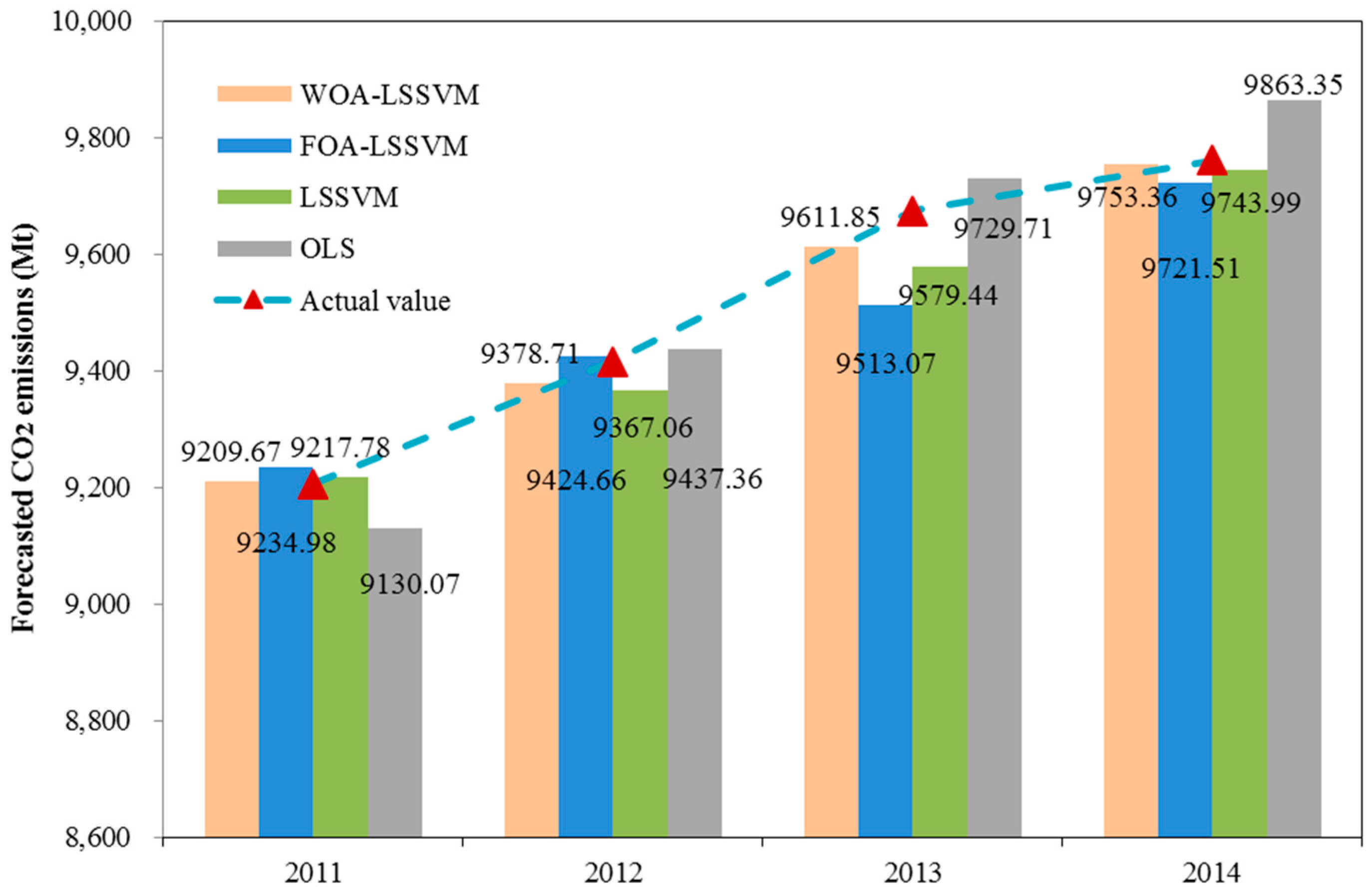
The actual data and prediction data for CO2 emissions in China by using WOA-LSSVM, FOA-LSSVM, LSSVM, and OLS methods during the period of 2011–2014 are illustrated in Figure 6. We can deduce that the WOA-LSSVM method performs best for CO2 emissions in 2011 and 2014 among all of the compared forecasting models. In 2013, the forecasted result attained from the OLS method has the smallest gap from the actual value, and the WOA-LSSVM model ranks second. In 2012, the forecasting result of FOA-LSSVM model is closest to the actual value, followed by OLS method, WOA-LSSVM, and single LSSVM models.
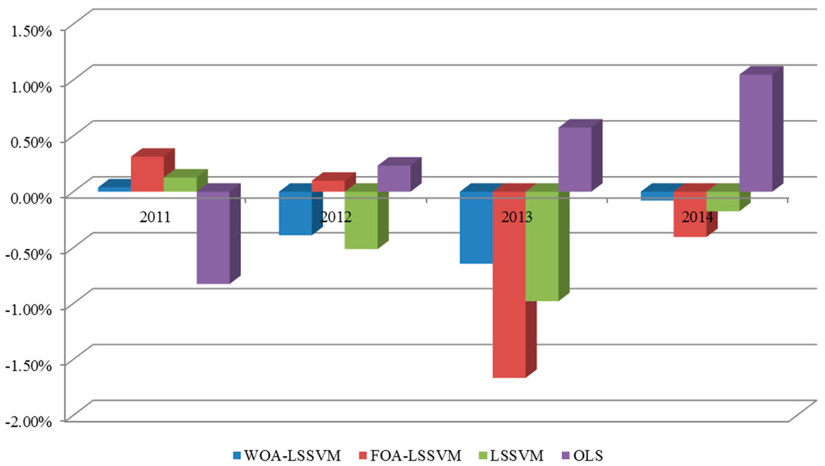
To accurately compare the CO2 emissions forecasting performances of different models, the evaluation indicators PE, MAPE, and RMSE are employed, and the results are demonstrated in Figure 7 and Table 4. Generally, the PE range in interval [−3%, 3%] is deemed as standard performance of forecasting results [34]. As can be seen from Figure 7, all of the prediction points are in the range of [−3%, 3%]. Meanwhile, the forecasting PEs of WOA-LSSVM model all fall within the scope of [−0.7%, 0.7%]. The proposed WOA-LSSVM model show the best CO2 emissions forecasting performance in 2011 and 2014 based on PE standard. Although the proposed WOA-LSSVM model does not reach the highest prediction accuracy in the remaining years based on PE standard, the gaps are small. Therefore, the WOA-LSSVM model has the superior CO2 emissions prediction performance compared to OLS, single LSSVM, and FOA-LSSVM models.
The calculation results listed in Table 4 also verify the superiority of WOA-LSSVM model in accordance with MAPE and RMSE. The MAPE value of WOA-LSSVM model is only 0.29%, which is the smallest among all of the compared models (0.62% of FOA-LSSVM, 0.45% of single LSSVM, and 0.67% of OLS model). The RMSE value of WOA-LSSVM approach is significantly less than that calculated by FOA-LSSVM, LSSVM, and OLS methods, which are 36.43 Mt, 84.34 Mt, 54.20 Mt, and 70.36 Mt, respectively. In this case, the prediction performance of WOA-LSSVM model is better than FOA-LSSVM, single LSSVM, and OLS. It is also very interesting to discover that the prediction precision of single LSSVM method is better than the FOA-LSSVM, but that the WOA-LSSVM has the best prediction performance. This implies that the WOA has a greater capacity for optimizing LSSVM-based CO2 emissions forecasting model than FOA. Therefore, it can be safely concluded that the WOA has great potential in optimizing parameters of LSSVM model for improving the CO2 emissions forecasting accuracy.
Conclusively, the established WOA-LSSVM approach can dramatically lessen the deviations between the actual CO2 emissions and prediction CO2 emissions, which is significantly superior to the single LSSVM, FOA-LSSVM, and OLS models in China’s CO2 emissions forecasting. As a new kind of nature-inspired meta-heuristic optimization algorithm, the WOA has the prospect for wide application.
5. Conclusions
The accurate and reliable prediction on CO2 emissions is of great significance for climate policy decision making and energy planning. In previous studies, it can be seen that the dramatic growth of CO2 emissions in China is driven by many factors. However, the nonlinear relationships of CO2 emissions with its driving forces are quite complicated, which makes the CO2 emissions forecasting a difficult task. Therefore, improving the accuracy of CO2 emissions forecasting is a field worth studying. In this study, the widely utilized LSSVM technique has been applied to build a new CO2 emissions forecasting model, the parameters of which are optimized by a latest nature-inspired meta-heuristic optimization algorithm, WOA. Meanwhile, the proposed WOA-LSSVM model takes the main driving factors including GDP, energy consumption and population as the input variables, which takes the social economic effects on CO2 emissions into consideration. To validate the potential of the presented WOA-LSSVM method in terms of CO2 emissions forecasting, three other models (namely FOA-LSSVM, single LSSVM, and OLS) are selected to compare the forecasting performance. The comparative analysis implies that the proposed WOA-LSSVM method show the best performance in China’s CO2 emissions forecasting based on three evaluation indicators (namely PE, MAPE and RMSE). The proposed WOA-LSSVM model is significantly superior to other selected models in terms of CO2 emissions forecasting, and the application of WOA to optimize LSSVM approach is valid and feasible. In future studies, the WOA, as a new nature-enlightened heuristic optimization algorithm, has the potential in optimizing other intelligent algorithms such as SVM and neural network for practical issues, such as electricity demand forecasting and renewable power output forecasting. In the meantime, we can also conduct research concentrating on scenario forecasting methods applied to CO2 emissions forecasting to give full consideration to the impacts of national policies, such as carbon-reduction policies, economic and social development levels, and human behaviors on CO2 emissions.
Acknowledgments
This paper is sponsored by the National Key R&D Program of China under Grant No. 2016YFB0900501, National Natural Science Foundation of China under Grant No. 71373076, the Fundamental Research Funds for the Central Universities under Grant No. 2017MS060 and 2017XS106.
Author Contributions
Huiru Zhao put forward the concept of this study. Haoran Zhao completed the paper. Sen Guo modified the final draft of the manuscript.
Conflicts of Interest
The authors declare no conflict of interest.
References
- Suganthi, L.; Samuel, A.A. Energy models for demand forecasting—A review. Renew. Sustain. Energy Rev. 2012, 16, 1223–1240. [Google Scholar] [CrossRef]
- Wang, W.; Kuang, Y.; Huang, N. Study on the decomposition of factors affecting energy-related carbon emissions in Guangdong province, China. Energies 2011, 4, 2249–2272. [Google Scholar] [CrossRef]
- Akbostancı, E.; Tunç, G.I.; Aşık, S.T. CO2 emissions of Turkish manufacturing industry: A decomposition analysis. Appl. Energy 2011, 88, 2273–2278. [Google Scholar] [CrossRef]
- Auffhammer, M.; Carson, R.T. Forecasting the path of China’s CO2 emissions using province-level information. J. Environ. Econ. Manag. 2008, 55, 229–247. [Google Scholar] [CrossRef]
- Safdarnejad, S.M.; Hedengren, J.D.; Baxter, L.L. Dynamic optimization of a hybrid system of energy-storing cryogenic carbon capture and a baseline power generation unit. Appl. Energy 2016, 172, 66–79. [Google Scholar] [CrossRef]
- Gopan, A.; Kumfer, B.M.; Phillips, J.; Thimsen, D.; Smith, R.; Axelbaum, R.L. Process design and performance analysis of a staged, pressurized oxy-combustion (SPOC) power plant for carbon capture. Appl. Energy 2014, 125, 179–188. [Google Scholar] [CrossRef]
- Safdarnejad, S.M.; Hedengren, J.D.; Baxter, L.L. Plant-level dynamic optimization of cryogenic carbon capture with conventional and renewable power sources. Appl. Energy 2015, 149, 354–366. [Google Scholar] [CrossRef]
- Kang, C.A.; Brandt, A.R.; Durlofsky, L.J. A new carbon capture proxy model for optimizing the design and time-varying operation of a coal-natural gas power station. Int. J. Greenh. Gas Control 2016, 48, 234–252. [Google Scholar] [CrossRef]
- Belaissaoui, B.; Cabot, G.; Cabot, M.S.; Willson, D.; Favre, E. CO2 capture for gas turbines: An integrated energy-efficient process combining combustion in oxygen-enriched air, flue gas recirculation, and membrane separation. Chem. Eng. Sci. 2013, 97, 256–263. [Google Scholar] [CrossRef]
- O’Neill, B.C.; Desai, M. Accuracy of past projections of US energy consumption. Energy Policy 2005, 33, 979–993. [Google Scholar] [CrossRef]
- Auffhammer, M. The rationality of EIA forecasts under symmetric and asymmetric loss. Resour. Energy Econ. 2007, 29, 102–121. [Google Scholar] [CrossRef]
- Bohringer, C.; Conrad, K.; Loschel, A. Carbon taxes and joint implementation: An applied general equilibrium analysis for Germany and India. Environ. Resour. Econ. 2003, 24, 49–76. [Google Scholar] [CrossRef]
- Meng, M.; Niu, D. Modeling CO2 emissions from fossil fuel combustion using the logistic equation. Energy 2011, 36, 3355–3359. [Google Scholar] [CrossRef]
- Liang, Q.M.; Fan, Y.; Wei, Y.M. Multi-regional input–output model for regional energy requirements and CO2 emissions in China. Energy Policy 2007, 35, 1685–1700. [Google Scholar] [CrossRef]
- Chen, T.; Wang, Y. A fuzzy-neural approach for global CO2 concentration forecasting. Intell. Data Anal. 2011, 15, 763–777. [Google Scholar]
- Pao, H.T.; Tsai, C.H. Modeling and forecasting the CO2 emissions, energy consumption, and economic growth in Brazil. Energy 2011, 36, 2450–2458. [Google Scholar] [CrossRef]
- Lin, C.S.; Liou, F.M.; Huang, C.P. Grey forecasting model for CO2 emissions: A Taiwan study. Appl. Energy 2011, 88, 3816–3820. [Google Scholar] [CrossRef]
- He, J.K.; Deng, J.L.; Su, M.S. CO2 emission from China’s energy sector and strategy for its control. Energy 2010, 35, 4494–4498. [Google Scholar] [CrossRef]
- Liao, R.J.; Zheng, H.B.; Grzybowski, S.; Yang, L.J. Particle swarm optimization-least squares support vector regression based forecasting model on dissolved gases in oil-filled power transformers. Electr. Power Syst. Res. 2011, 81, 2074–2080. [Google Scholar] [CrossRef]
- Wu, Q. Hybrid model based on wavelet support vector machine and modified genetic algorithm penalizing Gaussian noises for power load forecasts. Expert Syst. Appl. 2011, 38, 379–385. [Google Scholar] [CrossRef]
- Zhou, J.Y.; Shi, J.; Li, G. Fine tuning support vector machines for short-term wind speed forecasting. Energy Convers. Manag. 2011, 52, 1990–1998. [Google Scholar] [CrossRef]
- Wang, S.; Yu, L.; Tang, L.; Wang, S.Y. A novel seasonal decomposition based least squares support vector regression ensemble learning approach for hydropower consumption forecasting in China. Energy 2011, 36, 6542–6554. [Google Scholar] [CrossRef]
- Sulaimana, M.H.; Mustafab, M.W.; Shareefc, H.; Abd-Khalid, S.N. An application of artificial bee colony algorithm with least squares supports vector machine for real and reactive power tracing in deregulated power system. Int. J. Electr. Power 2012, 37, 67–77. [Google Scholar] [CrossRef]
- Dos Santosa, G.S.; Justi Luvizottob, L.G.; Marianib, V.C.; Dos Santos, L.C. Least squares support vector machines with tuning based on chaotic differential evolution approach applied to the identification of a thermal process. Expert Syst. Appl. 2012, 39, 4805–4812. [Google Scholar] [CrossRef]
- Li, H.; Guo, S.; Zhao, H.; Su, C.; Wang, B. Annual electric load forecasting by a least squares support vector machine with a fruit fly optimization algorithm. Energies 2012, 5, 4430–4445. [Google Scholar] [CrossRef]
- Mirjalili, S.; Lewis, A. The Whale optimization algorithm. Adv. Eng. Softw. 2016, 95, 51–67. [Google Scholar] [CrossRef]
- Huang, X.; Shi, L.; Suykens, J.A.K. Asymmetric least squares support vector machine classifiers. Comput. Stat Data Anal. 2014, 70, 395–405. [Google Scholar] [CrossRef]
- Watkins, W.A.; Schevill, W.E. Aerial observation of feeding behavior in four baleen whales: Eubalaena glacialis, Balaenoptera borealis, Megaptera novaean-gliae, and Balaenoptera physalus. J. Mammal. 1979, 60, 155–163. [Google Scholar] [CrossRef]
- Goldbogen, J.A.; Friedlaender, A.S.; Calambokidis, J.; Mckenna, M.F.; Simon, M.; Nowacek, D.P. Integrative approaches to the study of baleen whale diving behavior, feeding performance, and foraging ecology. BioScience 2013, 63, 90–100. [Google Scholar]
- Andresosso-O’Callaghan, B.; Yue, G. Sources of output change in China: 1987–1997 application of a structural decomposition analysis. Appl. Econ. 2002, 34, 2227–2237. [Google Scholar] [CrossRef]
- Peters, G.; Webber, C.; Guan, D.; Hubacek, K. China’s growing CO2 emissions a race between lifestyle changes and efficiency gains. Environ. Sci. Technol. 2007, 41, 5939–5944. [Google Scholar] [CrossRef]
- Guan, D.; Peters, G.P.; Weber, C.L.; Hubacek, K. Journey to world top emitter: An analysis of the driving forces of China’s recent CO2 emissions surge. Geophys. Res. Lett. 2009, 36, 1–5. [Google Scholar] [CrossRef]
- Wang, S.; Yang, J. A probabilistic model for latent least squares regression. Neurocomputing 2015, 149, 1155–1161. [Google Scholar] [CrossRef]
- Amiri, M.; Davande, H.; Sadeghian, A.; Chartier, S. Feedback associative memory based on a new hybrid model of generalized regression and self-feedback neural networks. Neural Netw. 2010, 23, 892–904. [Google Scholar] [CrossRef] [PubMed]
Figure 1.
Bubble-net predation strategy of humpback whales [26].
Figure 1.
Bubble-net predation strategy of humpback whales [26].

Figure 2.
The steps of WOA method.

Figure 3.
The procedure of the whale optimization algorithm of the least squares support vector machine (WOA-LSSVM) method for carbon dioxide (CO2) emissions prediction.
Figure 3.
The procedure of the whale optimization algorithm of the least squares support vector machine (WOA-LSSVM) method for carbon dioxide (CO2) emissions prediction.
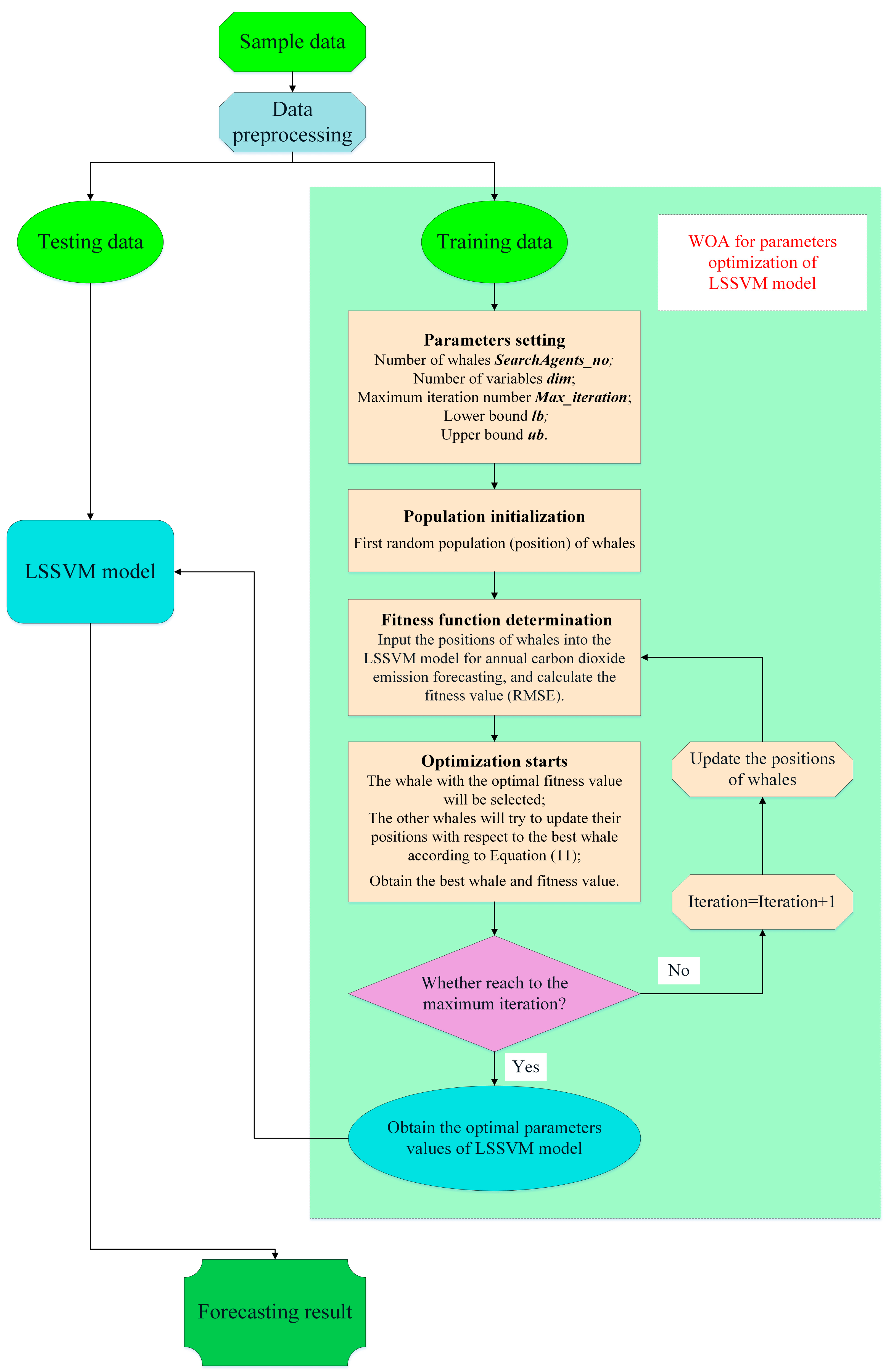
Figure 4.
The sample data of China’s CO2 emissions and selected driving factors.
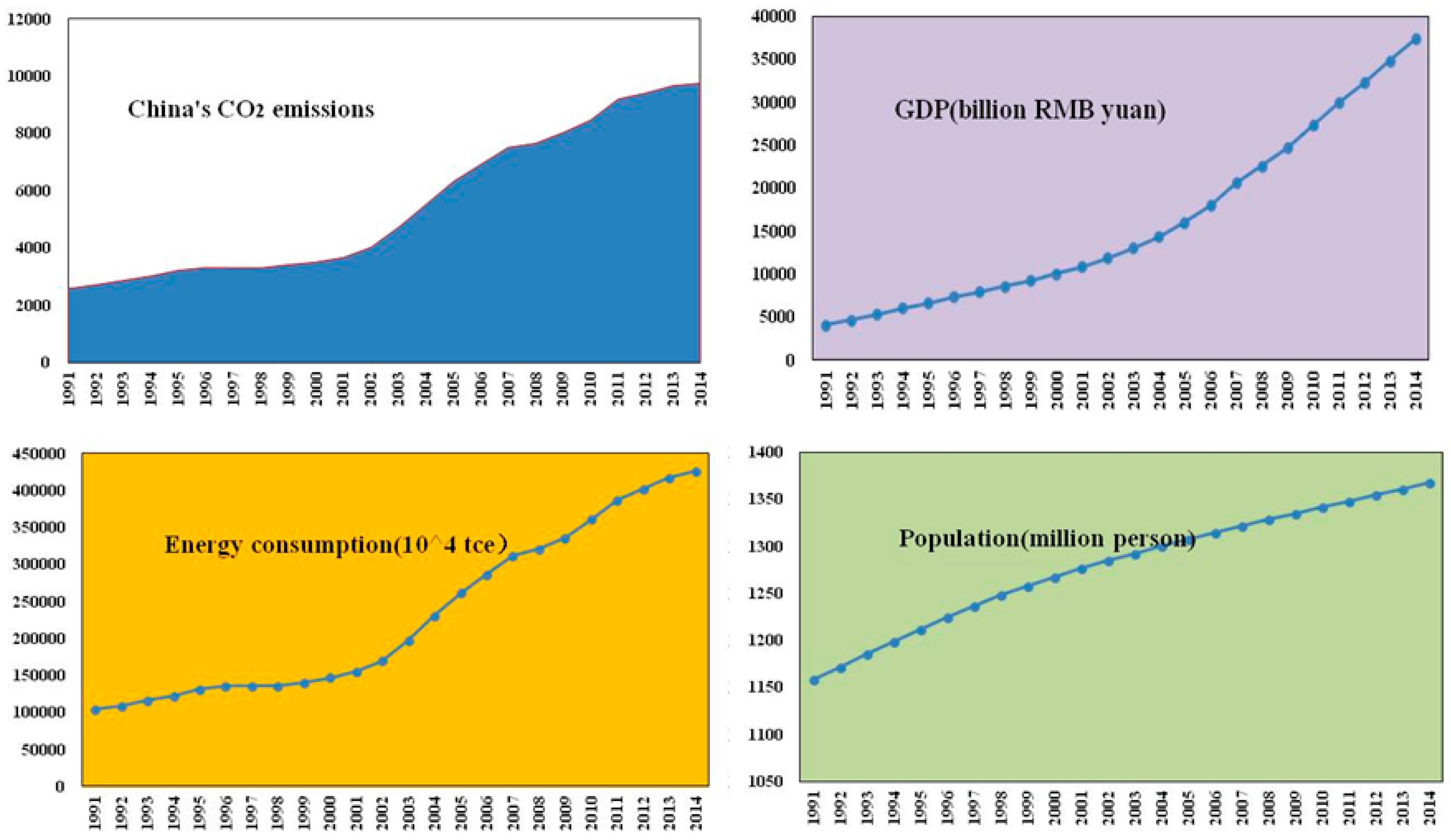
Figure 5.
The iterative root mean square error (RMSE) trend of the WOA-LSSVM method finding for optimized parameters.
Figure 5.
The iterative root mean square error (RMSE) trend of the WOA-LSSVM method finding for optimized parameters.
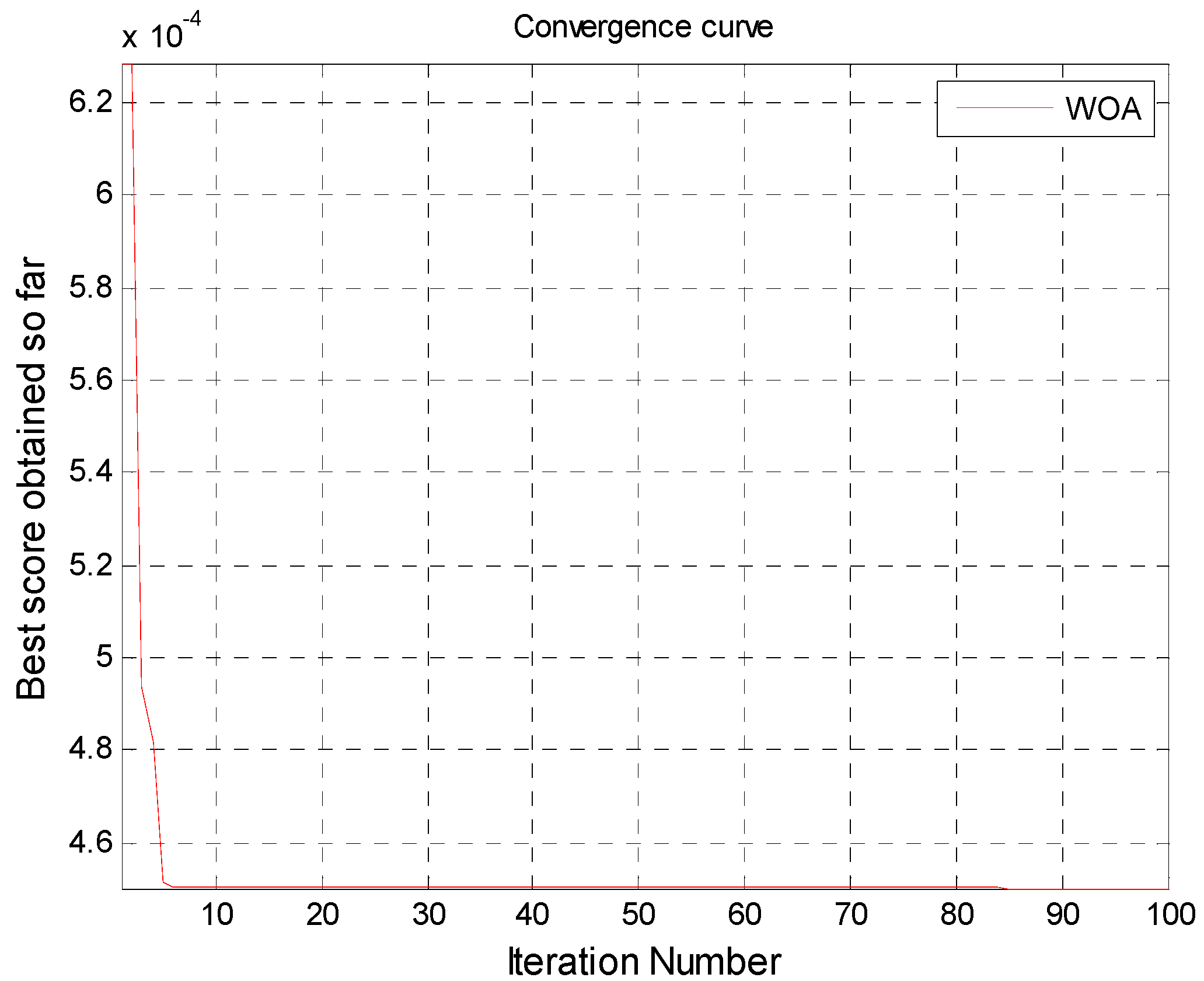
Figure 6.
Forecasting results of China’s CO2 emissions between 2011 and 2014 by using different models.
Figure 6.
Forecasting results of China’s CO2 emissions between 2011 and 2014 by using different models.

Figure 7.
Percentage error (PE) values of selected prediction methods.


Table 1.
The correlation degrees between China’s CO2 emissions and driving forces.
| Driving Forces | GDP | Energy Consumption | Population | Total Export | Economic Structure * |
|---|---|---|---|---|---|
| Correlation degree | 0.6577 | 0.6727 | 0.6798 | 0.6377 | 0.6015 |
* The economic structure is represented by the proportion of the secondary industry added value in GDP.
Table 2.
Forecasting results and gaps by using WOA-LSSVM model.
| Year | Forecasting Value (Unit: Mt) | Actual Value (Unit: Mt) | The Gap * (Unit: Mt) |
|---|---|---|---|
| 2011 | 9209.67 | 9206.12 | −3.55 |
| 2012 | 9378.71 | 9415.42 | 36.71 |
| 2013 | 9611.85 | 9674.22 | 62.37 |
| 2014 | 9753.36 | 9761.08 | 7.71 |
* The gap indicates the difference between the predicted value and actual value, the negative value of which demonstrates the actual data is less than the predicted one.
Table 3.
The determined values of parameters for fruit fly optimization (FOA)-LSSVM, single LSSVM model and WOA-LSSVM model.
Table 3.
The determined values of parameters for fruit fly optimization (FOA)-LSSVM, single LSSVM model and WOA-LSSVM model.
| Model | FOA-LSSVM | LSSVM | WOA-LSSVM |
|---|---|---|---|
| 0.2496 | 0.8 | 2.0684 | |
| C | 5.6947 | 20 | 93.2203 |
Table 4.
Mean absolute percentage error (MAPE) and RMSE for chosen prediction methods.
| Model | WOA-LSSVM | FOA-LSSVM | LSSVM | OLS |
|---|---|---|---|---|
| MAPE (%) | 0.29 | 0.62 | 0.45 | 0.67 |
| RMSE (Mt) | 36.43 | 84.34 | 54.20 | 70.36 |
© 2017 by the authors. Licensee MDPI, Basel, Switzerland. This article is an open access article distributed under the terms and conditions of the Creative Commons Attribution (CC BY) license (http://creativecommons.org/licenses/by/4.0/).
Share and Cite
MDPI and ACS Style
Zhao, H.; Guo, S.; Zhao, H. Energy-Related CO2 Emissions Forecasting Using an Improved LSSVM Model Optimized by Whale Optimization Algorithm. Energies 2017, 10, 874. https://doi.org/10.3390/en10070874
AMA Style
Zhao H, Guo S, Zhao H. Energy-Related CO2 Emissions Forecasting Using an Improved LSSVM Model Optimized by Whale Optimization Algorithm. Energies. 2017; 10(7):874. https://doi.org/10.3390/en10070874
Chicago/Turabian StyleZhao, Haoran, Sen Guo, and Huiru Zhao. 2017. "Energy-Related CO2 Emissions Forecasting Using an Improved LSSVM Model Optimized by Whale Optimization Algorithm" Energies 10, no. 7: 874. https://doi.org/10.3390/en10070874
Note that from the first issue of 2016, this journal uses article numbers instead of page numbers. See further details here.