
Impact Analysis of Demand Response Intensity and Energy Storage Size on Operation of Networked Microgrids


Department of Electrical Engineering, Incheon National University, 12-1 Songdo-dong, Yeonsu-gu, Incheon 406840, Korea
*
Author to whom correspondence should be addressed.
Energies 2017, 10(7), 882; https://doi.org/10.3390/en10070882
Submission received: 17 May 2017
/
Revised: 19 June 2017
/
Accepted: 27 June 2017
/
Published: 30 June 2017
(This article belongs to the Special Issue Battery Energy Storage Applications in Smart Grid)
Abstract
:Integration of demand response (DR) programs and battery energy storage system (BESS) in microgrids are beneficial for both microgrid owners and consumers. The intensity of DR programs and BESS size can alter the operation of microgrids. Meanwhile, the optimal size for BESS units is linked with the uncertainties associated with renewable energy sources and load variations. Similarly, the participation of enrolled customers in DR programs is also uncertain and, among various other factors, uncertainty in market prices is a major cause. Therefore, in this paper, the impact of DR program intensity and BESS size on the operation of networked microgrids is analyzed while considering the prevailing uncertainties. The uncertainties associated with forecast load values, output of renewable generators, and market price are realized via the robust optimization method. Robust optimization has the capability to provide immunity against the worst-case scenario, provided the uncertainties lie within the specified bounds. The worst-case scenario of the prevailing uncertainties is considered for evaluating the feasibility of the proposed method. The two representative categories of DR programs, i.e., price-based and incentive-based DR programs are considered. The impact of change in DR intensity and BESS size on operation cost of the microgrid network, external power trading, internal power transfer, load profile of the network, and state-of-charge (SOC) of battery energy storage system (BESS) units is analyzed. Simulation results are analyzed to determine the integration of favorable DR program and/or BESS units for different microgrid networks with diverse objectives.
1. Introduction
A microgrid is an integration of distributed energy sources, energy storage systems, and local demand. The demand of a microgrid could be controllable (curtailable and shiftable) and/or non-controllable [1]. Recently, the interconnection of various microgrids to form a network of microgrid has emerged as an application and advanced form of the single microgrid concept [2]. The operation of single/networked microgrids is challenging due to the involvement of various complex factors like the intermittent nature of renewable energy sources, demand fluctuations, uncertain market prices, and extreme weather conditions [3]. In the last decade, the operation of microgrids considering various prevailing uncertainties has been an active research field for researchers.
The major uncertainties considered in the literature can be categorized as the uncertainties related to the renewable energy sources [4,5], forecasted loads [6,7], both renewable energy sources and loads [8,9], and demand response (DR) programs [10,11]. Various uncertainty-modeling techniques have been used by different researchers for realizing the abovementioned uncertainties. The major techniques available in the literature can be categorized as stochastic modeling [12], robust optimization [13], and fuzzy modeling [14]. There are various merits and demerits of each technique, which can be found in [8,9]. Robust optimization has gained popularity over various other uncertainty-modeling techniques due to its ability to provide immunity against the worst-case uncertainty realization. In addition, the computational burden is reduced in robust optimization due to consideration of uncertainty bounds only. Due to the abovementioned merits, various forms of robust optimization have been used for the optimal operation of microgrids [8,9,13,15].
Integration of energy storage systems is necessary for microgrids to compensate for the uncertainties of renewable energy sources, increase the profit for microgrids, and increase service reliability to the consumers [16]. The major energy storage technologies being used for microgrids are summarized in [17], among which battery energy storage systems (BESS) are the most widely used technology. BESS have the capability to achieve these objectives by absorbing surplus power from renewables, buying power from the utility grid during off-peak hours and selling back at peak hours, and supporting local supply during system contingencies. In order to achieve these benefits, optimal sizing and siting of BESS units are required [18]. Various studies have been conducted for the optimal siting of BESSs for microgrids. Cost-benefit analysis has been conducted by [19] to determine the optimal sizing of energy storage systems in microgrids. A multi-objective optimal allocation model of BESS has been developed by [20] for maximum photovoltaic consumptive rate, along with annual net profits. The impact of BESS on voltage and frequency stability of microgrids has been analyzed by [21]. A BESS control model is proposed by [22] by considering BESS as an equivalent fuel-run generator and enabling it for use in the unit commitment of microgrids.
In addition to BESS, DR programs can also be used to overcome the challenges associated with the operation of microgrids. DR programs can be used by the utilities for managing the consumption behavior of consumers in response to supply conditions. DR has the capability to benefit utilities, regional transmission organizations (RTOs), independent system operators (ISOs), and end users. In order to benefit from the DR, various studies have been conducted for integration of DR programs in the operation of microgrids. Both DR programs and distributed generation units are used for compensating renewable forecast errors by [23] and incentive-based DR programs are considered by [24] for the scheduling of microgrids. An algorithm is proposed by [25] for the efficient management of event-based DR program in microgrids. A central DR program is proposed by [26] for frequency regulation and manipulated load minimization for microgrids. A multi-agent based DR program for industrial loads has been analyzed by [27] for optimal operation of microgrids using a central controller. A summary of the available approaches is presented in Table 1.
Optimal sizing and siting of BESS units have been widely studied in the literature, as mentioned in the previous paragraphs. Similarly, integration of various DR programs has also been widely studied for microgrids in the literature. However, the optimal size of BESS units is significantly affected by the uncertainties associated with renewable energy sources and load variations. Similarly, the participation of enrolled customers in DR programs is also uncertain. In addition, uncertainty in market price signals can affect the participation rate of enrolled customers. The size of BESS units and participation rate of enrolled customers (DR intensity) can affect the operation of microgrids. Therefore, the effects of variations in BESS size and DR intensity on the operation of microgrids need to be investigated to find an acceptable range for integration in microgrids.
In this paper, similar to [28], the impact of price-based DR programs, incentive-based DR programs, and BESS size on the operation of microgrid networks is analyzed. The effect of simultaneous change in DR program intensity and BESS size is also analyzed. In all cases, change in operation cost of the microgrid network, internal power transfer, external power trading, load profile of the network, and state-of-charge (SOC) of BESS units are analyzed. In contrast to [28], the uncertainties related to forecasted values of loads, output power of renewable power sources, and market price signals are realized by using the robust optimization method. Robust optimization has the capability to provide immunity against the worst-case scenario if the uncertainties lie within the specified bounds. The worst-case scenario of prevailing uncertainties is considered for evaluating the feasibility of the proposed method. Incentive-based DR programs are only triggered during specified intervals, defined by the utility grid. In addition, the maximum amount of load that can be shifted to a specific time interval is also constrained by the maximum intake capability of that interval. The major contributions of this study can be summarized as follows:
- In contrast to the existing literature, where sizing/siting of BESS and integration of DR programs are focused, the impact of change in BESS size and DR intensity on the operation of microgrids is considered in this study.
- Robust optimization is used and worst-case scenarios of renewables, loads, and price signals are considered for analyzing the impact of BESS size and DR intensity on the operation of microgrids.
- Finally, integration of favorable DR program and/or BESS units for different microgrid networks with diverse objectives is suggested by using simulation results.
2. Demand Response and Energy Storage for Networked Microgrids
2.1. Demand Response (DR) Programs and Battery Energy Storage System (BESS)
The demand response programs can be categorized into various categories based on their application horizon, incentive type, penalty enforcement, etc. An overview of different DR programs is shown in Figure 1. All the demand response programs can be broadly divided into price-based DR programs and incentive-based DR programs [29]. In the case of price-based DR programs, market price signals are varied over different periods and incentive-based DR programs are devised to incentivize the participants for curtailing their loads during system contingencies. Figure 1 shows that there are various programs in both price-based and incentive-based DR categories. However, the objective of all price-based DR programs is to allow customers to shift their loads from peak hours to non-peak hours. Similarly, the objective of all the incentive-based DR programs is to curtail loads during system contingencies.
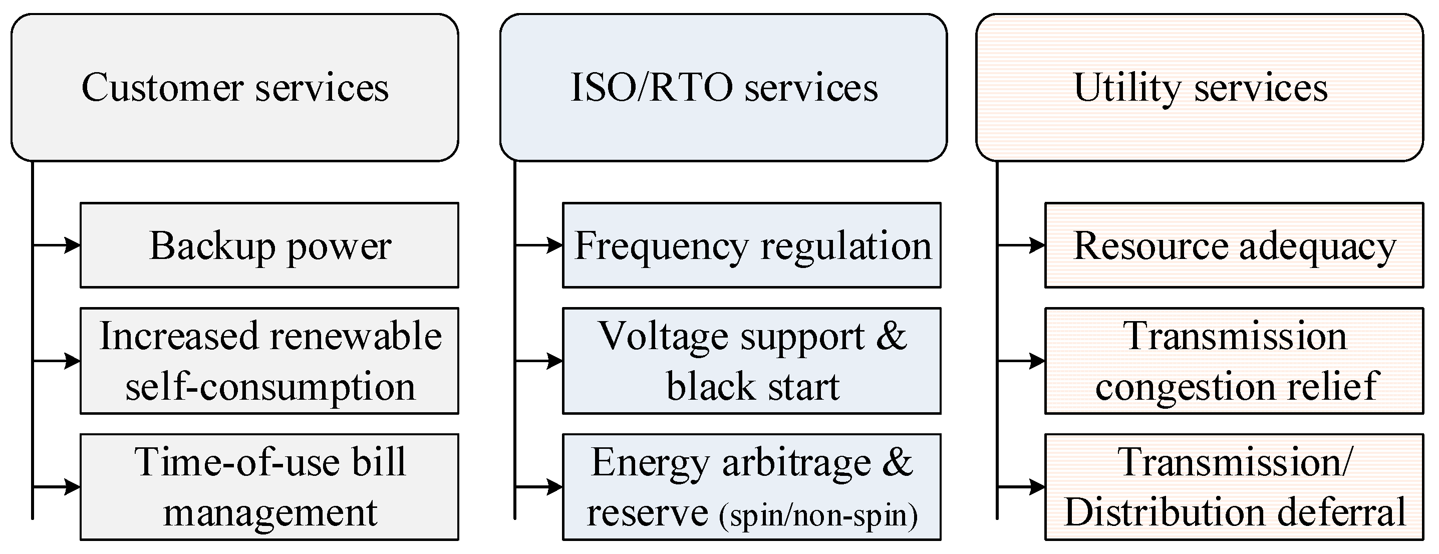
Similar to DR programs, BESS also has the capability to benefit not only the utilities but also the ISOs, RTOs, and end users [30]. An overview of different services, which can be achieved by integrating BESS units for different stakeholders in the power industry, is provided in Figure 2. BESS has the capability to absorb surplus power from renewables, which can be used for trading with the utility grid or for feeding loads during peak load intervals. Similarly, BESS can be used for buying power from the utility grid during off-peak price intervals and selling it back to the grid during peak-price intervals, which will benefit both the utility grid and the microgrid owners. DR programs and ESS can be used to reshape the load profiles, reduce the stress on the grid during peak periods, and decrease the operation cost of microgrids.
2.2. System Configuration
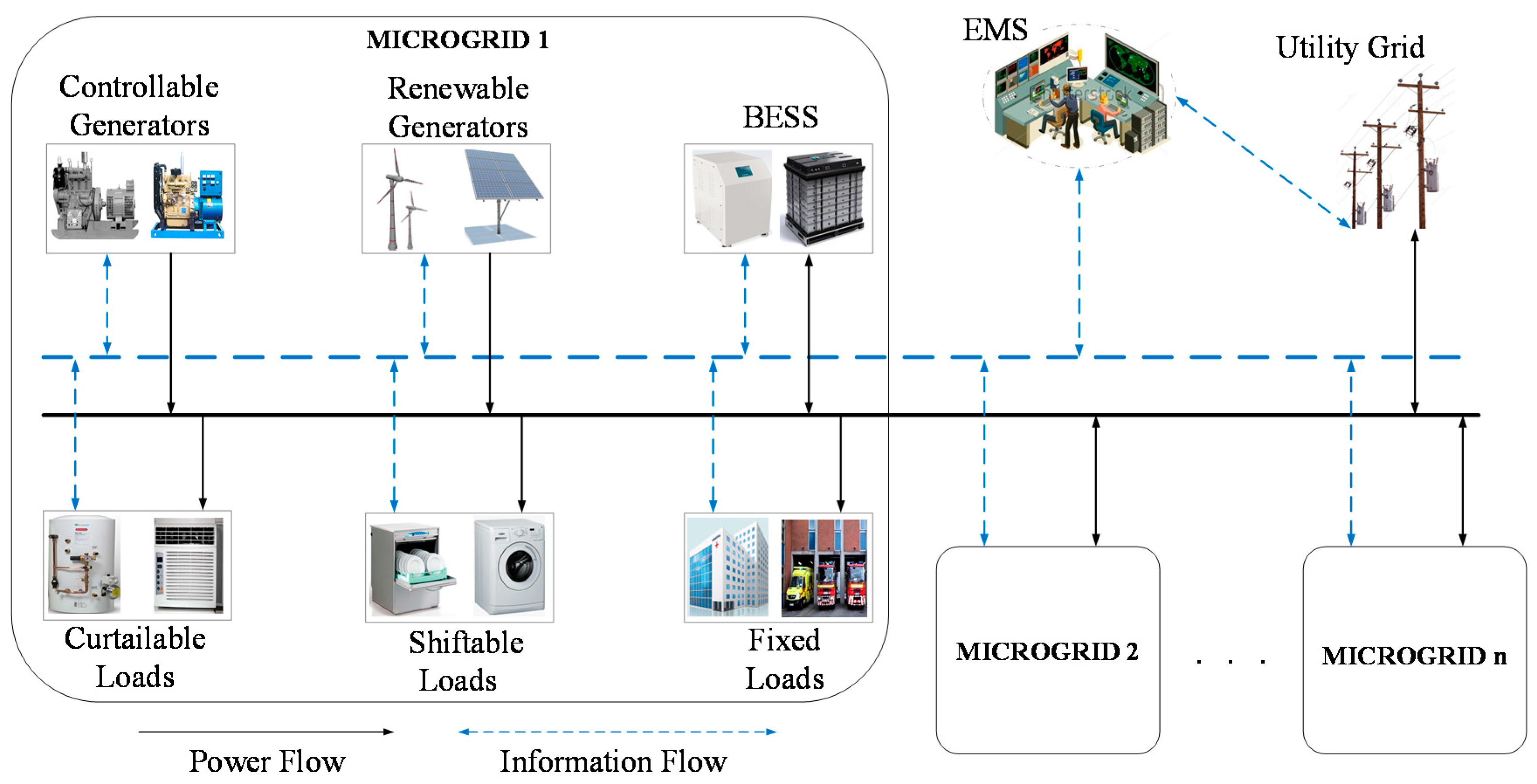
A typical networked microgrid, which is also considered in this study, is shown in Figure 3. Each microgrid contains controllable distributed generators (CDGs), renewable distributed generators (RDGs), BESS, and loads. All the microgrids contain diesel generators as CDG units. Microgrid 1 contains a wind turbine as an RDG unit, while microgrid 2 and microgrid 3 contain photovoltaic cells as RDG units. Similar to [10], loads in each microgrid are decomposed into fixed load, shiftable load, and curtailable load, and each load category is defined as follows:
- Fixed Loads: These loads are considered the most critical as they can be neither curtailed nor shifted. These loads cannot participate in any DR program and need to be served by the microgrid.
- Controllable Loads: These loads are considered less critical than fixed loads and are divided into shiftable loads and curtailable loads. Only controllable loads can participate in different DR programs offered by the utilities or RTOs/ISOs.
- Shiftable Loads: These loads are a sub-category of controllable loads, which can be shifted from one time interval to another time interval but cannot be curtailed, i.e., can participate in price-based DR programs only.
- Curtailable Loads: These loads are also a sub-category of controllable loads, which can be curtailed when the market price is very high or system stability is jeopardized, i.e., can participate in incentive-based DR programs.
An energy management system (EMS) is an important part of microgrids and plays a vital role in the operation of single/networked microgrids. Therefore, various EMS strategies have been investigated by the research community in the literature. Due to the merits of cooperative networked microgrid communities highlighted by [31,32], a cooperative microgrid community is considered in this study. A centralized EMS is utilized for scheduling the resources of the entire network. Each of the microgrids initially receives the market price signals (buying and selling prices) along with the peak price intervals information. In the first step, each microgrid reshapes its load profile by using the information of the utility grid, generation cost of local CDGs, and output of RDGs. The reshaped load profiles are sent to the EMS. EMS is responsible for receiving information from all the microgrids and for optimally scheduling all the resources while considering the controllable loads. Due to the networking of microgrids, power transfer among microgrids of the network is possible. EMS is responsible for deciding the power transfer among the microgrids of the network. Similarly, all the microgrids can trade power with the utility grid and the trading amount is also decided by the EMS.
3. Problem Formulation
In this section, a mathematical model for a network of microgrids is developed. The total microgrids in the network are assumed to be M, where M could be any finite integer number. Throughout the modeling, m is used as an indicator for microgrid number, i.e., m M. Therefore, the developed model can be extended for any finite number of microgrids, i.e., M.
3.1. Deterministic Model
The first step is to formulate a deterministic model for the microgrid network. Uncertainty models for renewable energy sources, loads, and market price signals are formulated in the next sections. Transformed uncertainty models are incorporated in the original deterministic model to obtain a tractable robust counterpart. The tractable robust counterpart can be implemented using commercial optimization tools like CPLEX.
3.1.1. Objective Function
The first term of the objective function of the deterministic model contains the generation costs, start-up, and shutdown costs of CDGs of all the microgrids. The second term contains the total profit gained by the microgrid network by trading electricity with the utility grid. The third term contains the penalty cost for shifting load from interval t to t’. The fourth term contains the incentive for curtailing loads by mth microgrid. is one (1) if load shifting is allowed and is infinity (a very large value) otherwise.
3.1.2. Load Balancing Constraints
In each microgrid, the adjusted load amount needs to be balanced by the generation of CDG units, RDGs, BESS charging/discharging, power transferred among microgrids, and power trading with the utility grid, as given by Equation (2). The adjusted load in each microgrid at time t can be computed using Equation (3). It contains fixed load, curtailable load, shiftable load, the amount of load shifted from other time intervals (t’) to t, and the amount of load shifted from t to other time intervals.
3.1.3. Constraints for Controllable Generators
Equations (4)–(8) show the constraints for dispatchable generators. In Equation (4), indicates the commitment status of in at time If the CDG is committed to operate at time , it takes the value of and otherwise. Equation (5) gives the upper and lower generation limits of gth CDG in mth microgrid. Equations (6) and (7) can be used to indicate startup and shutdown of gth CDG in mth microgrid at time t. Equation (8) shows that simultaneous startup and shutdown of a given CDG is not possible.
3.1.4. Energy Trading Constraints
The power trading between a microgrid m and the utility grid is limited by the maximum capacity of the line connecting them, as given by Equation (9). If any microgrid buys power from utility grid at t, the value of will be positive and vice versa. Similarly, constraints for transferring power from microgrid m to microgrid n at a given time interval t are given by Equations (10) and (11). Equation (12) shows that any microgrid can receive only a deficit amount of power from other microgrids and Equation (13) shows that only surplus power can be sent to other microgrids. Finally, Equation (14) shows that the total amount of power transferred among the microgrids of the network should be balanced.
3.1.5. Battery Constraints
The SOC limits of BESS unit in mth microgrid are given by Equation (15). Equation (16) shows that SOC at any time interval t depends upon the amount of electricity charged/discharged at that time interval and the SOC of the previous time step. The chargeable amount at any time interval t can be computed using Equation (17) and dischargeable amount at t by Equation (18). Equation (19) shows that at the beginning of the scheduling horizon, the SOC of the previous time step is equal to the initial SOC of the BESS. Finally, Equation (20) shows that simultaneous charging and discharging of BESS is not possible.
3.1.6. Demand Response Constraints
The total amount of load shifted from all other time intervals () to time interval t is constrained by Equation (21). Similarly, the amount of load shifted from time interval t to all other time intervals is constrained by Equation (22). is zero if shifting from t to t’ is allowed and is set to a very high value (); otherwise, it is as given by Equation (23). Finally, the amount of curtailable load at a given microgrid m at time t is constrained by Equation (24).
3.2. Uncertainty Modeling of Renewables and Loads
3.2.1. Uncertain Variables and Uncertainty Bounds
In the load balancing equation of deterministic model, the output power of renewable energy sources and adjusted load amount are uncertain. In the remaining part of the paper, only load will be used for adjustable load for the sake of simplicity. The bounded variables for load () are given by Equation (25) and renewables power generations () by Equation (26). The uncertainty bounds for load and renewables are also given by Equations (25) and (26). Where, and are lower and upper uncertainty bounds for load and and are lower and upper uncertainty bounds for renewables.
3.2.2. Worst-Case Identification and Problem Transformation
Similar to [8], the worst-case uncertainty scenario is identified and modeled. The worst-case () will occur for the load balancing of deterministic model (2), when the load takes the upper uncertainty bound and renewables take lower uncertainty bounds, as given by (27).
It can be observed from Equation (27) that maximization of uncertainty is another objective function inside the load balancing equation. Therefore, it will be treated as a sub-problem with the following constraints. is called the budget of uncertainty, which is used to control the conservatism of the solution.
This formulation results in a min-max problem. Therefore, the dual sub-problem is computed by using the method suggested by [13]. By applying the linear duality theory, following equations can be formulated. Equation (30) is the objective function of the dual problem and Equations (31)–(33) are the constraints.
3.2.3. Trackable Robust Load Balancing
In the final step of uncertainty modeling of renewables and loads, the dual problem is added to the load balancing equation of the deterministic model. Objective function at this stage is identical to that of the deterministic model. The robust trackable load balancing equation is updated as follows:
The objective function is constrained to all the constraints mentioned in the deterministic model, i.e., Equations (3)–(24). In addition, the objective function at this stage is also constrained by Equations (31)–(33).
3.3. Uncertainty Modeling of Buying and Selling Prices
3.3.1. Uncertain Variables and Uncertainty Bounds
The market buying price () and market selling price () signals in the objective function of the deterministic model are also uncertain. Similar to [33], the uncertainty deviations for buying and selling price signals are computed by using Equations (35)–(37). In Equation (35), is the deviation of the buying price signal from the nominal values. Similarly, in Equation (36), represents the deviation of the selling price signal. The constraints for uncertainty bounds for buying and selling price signals are given by Equation (28), which can by calculated by using the methods proposed by [33].
3.3.2. Robust Counterpart and Dual Problem
The robust counterpart of buying price signal is computed by using the method proposed by [33], as shown in Equations (38) and (39). Similarly, the robust counterpart of selling part is given by Equations (40) and (41).
Subject to
Equations (2) and (3)
Subject to
Equations (2) and (3).
These robust counterparts make min-max problem formulations. Therefore, the dual of both the inner sub-problems can be computed. The inner maximization problem is taken as an objective function and an equivalent mixed integer problem (MIP) formulation is computed, as suggested by [33].
Subject to
The dual for the buying part is given by Equations (42)–(45) and that of selling by Equations (46)–(49). and are defined as the budget of uncertainty for buying and selling prices, respectively. These variables can be used to control the conservatism and unfeasibility of the solution.
Subject to
3.4. Final Tractable Robust Counterpart
The final tractable robust counterpart is obtained by incorporating the dual of buying and selling price signals in the objective function and dual of renewables and load in the load balancing equation of the deterministic mode. The final tractable objective function is given by Equation (50) and the load balancing is given by Equation (51). The final tractable robust counterpart is a mixed integer linear programming problem, which can be easily implemented by using commercially available tools like CPLEX.
Subject to
Equations (3)–(24), (31)–(33), (35)–(37), (43)–(45), (47)–(49).
4. Numerical Simulations
The developed robust optimization model is applied to a microgrid network comprised of three microgrids, as shown in Figure 3. Each microgrid contains a CDG unit, a BESS unit, and an RDG unit, along with controllable and fixed loads. The operation horizon for the test cases is taken as 24 h, with a time interval of one hour. Simulations are carried out in CPLEX 12.3 in Java environment.
4.1. Input Data
The controllable load in each microgrid is divided into a shiftable (price-based DR) load and a curtailable load (incentive-based DR). The maximum and minimum amounts of both price-based and incentive-based DRs, as a function of total load, in each microgrid are shown in Table 2. Similarly, the maximum capacity of BESSs in all the microgrids is also tabulated in Table 2. The upper and lower bounds for all the uncertain quantities (renewable power, loads, and market price signals) are tabulated in Table 3. The maximum and minimum generation limits of CDGs in each microgrid are tabulated in Table 4. Finally, the capacities of power lines, which constrain the trading of power among microgrids of the network and with the utility grid, are tabulated in Table 4. The configuration assumptions and decision parameter values are taken as follows:
- It is assumed that each microgrid contains at least one BESS unit and has both shiftable and curtailable loads, i.e., controllable loads.
- A community EMS (CEMS) is assumed to be responsible for the operation of the entire multi-microgrid network.
- Each microgrid (MG) is assumed to have a BESS unit with a maximum capacity of 250 kWh.
- The maximum intensity of price-based DR programs and incentive-based DR programs is assumed to be 25% and 15% of the forecasted load, respectively, at each time interval.
- Incentive-based DR programs are assumed to be triggered in only peak-price intervals, i.e., 12 to 18 in this study.
- The uncertainty bounds for load, market price signals, and renewables are taken as ±10%, ±15%, and ±20%, respectively.
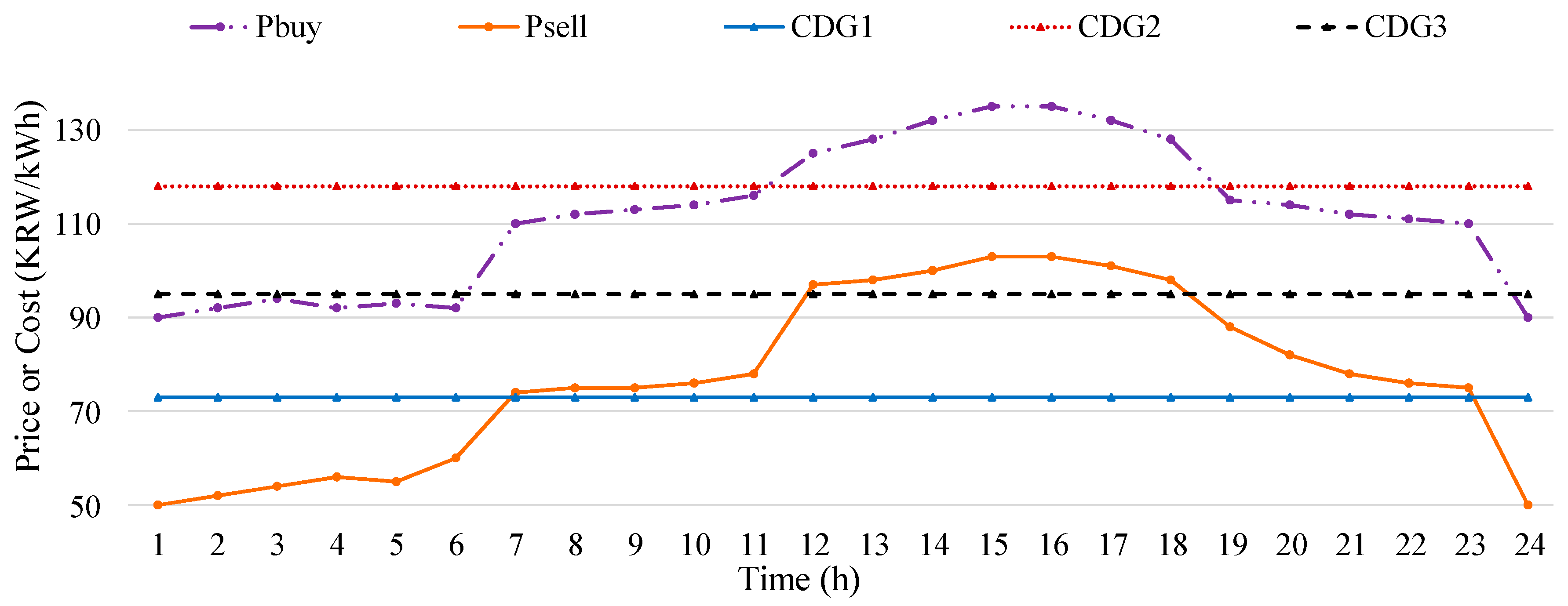
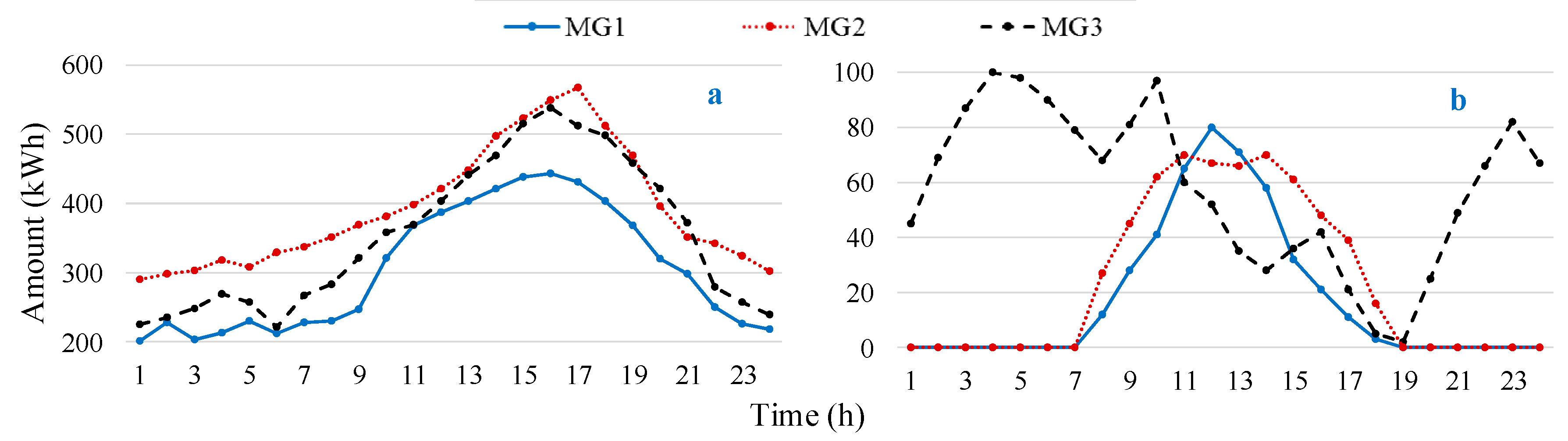
The real-time market price signals are taken as inputs and are shown in Figure 4 along with the generation cost of CDGs in each microgrid. Similarly, the hourly load profiles and output of renewable power sources of all the microgrids are shown in Figure 5. Figure 4 and Figure 5 show the worst-case values of all the uncertain variables. The nominal values can be obtained by using the uncertainty bounds shown in Table 3.
The effectiveness and applicability of the proposed method are evaluated by simulating three different cases in this study. In the first case, the DR intensity of both time-based DR and incentive-based DR is varied while setting the BESS capacity to zero. In the second case, the BESS capacity in each microgrid is varied while setting the DR intensity to zero. Finally, in the third case, both DR intensity and BESS capacity are varied in accordance with the maximum and minimum limits defined in Table 3. In all cases, the effect of each variable quantity on generation pattern of CDGs, load profiles of microgrids, internal power transfer (power transfer among microgrids), external power trading (power trading with the utility grid), BESS scheduling, and operation cost of the network are analyzed. In all cases, the worst-case values of uncertain parameters are considered. If the uncertainties lie within the specified bounds of Table 3, the developed model can provide a feasible solution.
4.2. Impact Analysis of DR Intensity
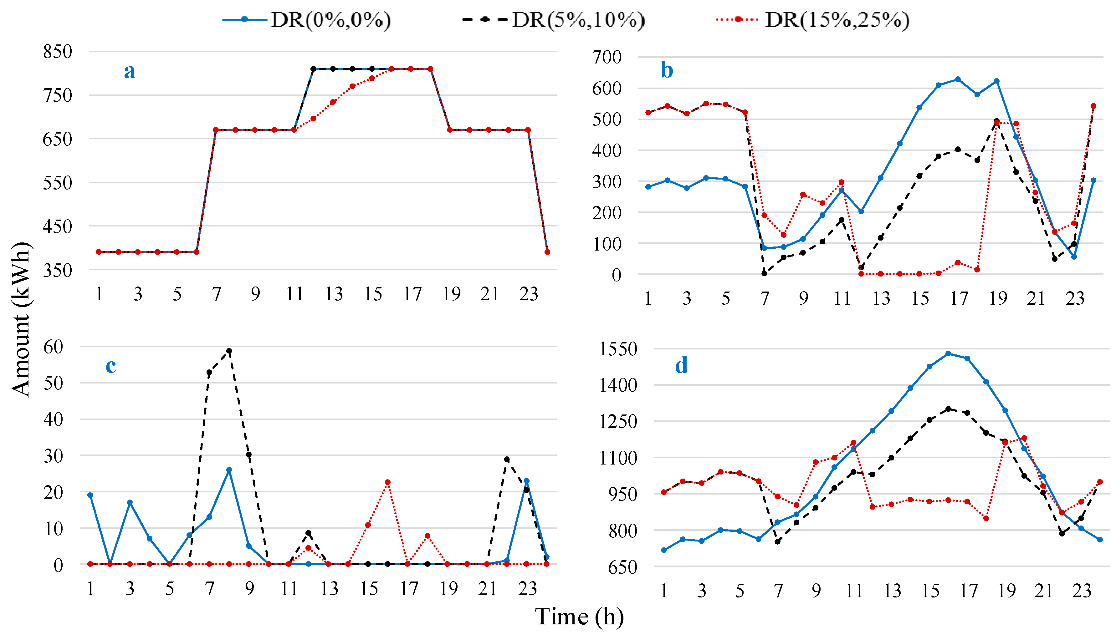
In this section, both price-based DR and incentive-based DR are considered and the impact of DR intensity is analyzed by considering three different cases. BESS size is taken as zero for all three cases in this section. The first term inside the parentheses in the legend of Figure 6 indicates the intensity of incentive-based DR and the second term indicates the intensity of price-based DR. The first case is the nominal case, where the intensity of both the DR programs is taken as zero. In the second case, the intensity of incentive-based DR is taken as 5% and the price-based DR as 10%. In the third case, both the DR programs have taken their highest values (15% and 25%), as mentioned in Table 2. The impact of different DR intensities on generation patterns of CDGs, power transfer among microgrids of the network, power trading with the utility grid, and load profiles of microgrids is analyzed. For the sake of visibility, the accumulated results of the entire network are shown in Figure 6.
Figure 6a shows that the generation pattern of CDGs is the same for the first and second cases, while in the third case the generation amount is reduced in the peak intervals. This reduction is due to a higher intensity of both DR programs during peak-price intervals. In the third case, due to a higher intensity of shiftable loads, more loads are shifted from peak hours to non-peak hours. Similarly, the intensity of curtailable loads is also increased; hence, more loads have participated to get incentives. In the first case, less electricity is bought from the utility grid during off-peak hours and more electricity is bought in the peak hours, as shown in Figure 6b. However, in the second case, less electricity is bought during peak price hours, while buying during off-peak hours has increased. This is due to a shifting of loads from peak to non-peak hours and curtailing of loads during peak price hours. Finally, in the third case, the amount of buying during peak hours has been reduced almost to zero and more electricity is bought during off-peak and shoulder peak intervals. Figure 6c shows that internal trading has reduced with the increase in DR intensity. In the first case, the load profile of the network has a peak during time intervals 12–18, as shown in Figure 6d. The peak has reduced for the second case and further reduced for the third case due to the higher intensity of DR programs. It can be observed from Figure 6d that the load magnitude of the remaining hours has increased for the second and the third cases due to a higher intensity of shiftable loads.
The intensity of DR in each microgrid is varied for six different cases and the summary of one day’s operation is tabulated in Table 5.
It can be observed that net external trading has been reduced with an increase in DR intensity due to the presence of curtailable loads. Table 5 also shows a reduction in the daily operation costs of the network with an increase in the DR intensity. The net internal trading does not follow a specific trend due to the changing of the load profile of individual microgrids with the change in DR intensity.
4.3. Impact Analysis of BESS Size
In this section, the size of BESS is varied from 0 kWh to 250 kWh in each microgrid of the network and three different cases are considered. The intensity of both the price-based DR and incentive-based DR programs is set to zero in this section. The first case is the nominal case, where the size of BESS in each microgrid is set to 0 kWh. In the second case, BESS size is set to 100 kWh and in the third case, BESS size is set to 250 kWh for each microgrid of the network. The impact of BESS size on the generation pattern of CDGs, power transfer among microgrids of the network, and power trading with the utility grid is analyzed. BESS size does not influence the load pattern of microgrids; therefore, the load profile of microgrids is not shown in Figure 7. Accumulated results of all microgrids are shown in Figure 7, for the sake of visibility.
The generation pattern of CDGs has remained the same for all three cases due to the same load profile of the network, as shown in Figure 7a. External trading has increased during initial off-peak price intervals with the increase in BESS size, as shown in Figure 7b. This increase reflects the fact that, during initial off-peak hours, more electricity is bought from the utility grid for charging BESS units. Contrarily, external trading has reduced during peak price intervals. This reduction indicates that BESS units are discharged during peak price intervals and buying from the utility grid has reduced.
Internal power transfer has reduced with the increase in BESS size due to an increase in self-reliance, as shown in Figure 7c. Figure 7d shows that BESS units are charged during initial off-peak hours and are discharged during peak hours for reducing the operation costs of the microgrid network. It can be observed from Figure 7b,d that the SOC of BESS units is in accordance with the external trading.
Six different cases are simulated by varying the BESS size in each microgrid with a step of 50 kWh. The impact of BESS size in each case is analyzed against the daily operation of the network and the summary is tabulated in Table 6. Net total internal power transfer has reduced with the increase in BESS size due to the increase in self-reliance of each microgrid. However, net external power trading has increased with the increase in BESS size. Finally, the daily operation costs have decreased with the increase in BESS size with a linear slope.
4.4. Impact Analysis of Both DR Intensity and BESS Size
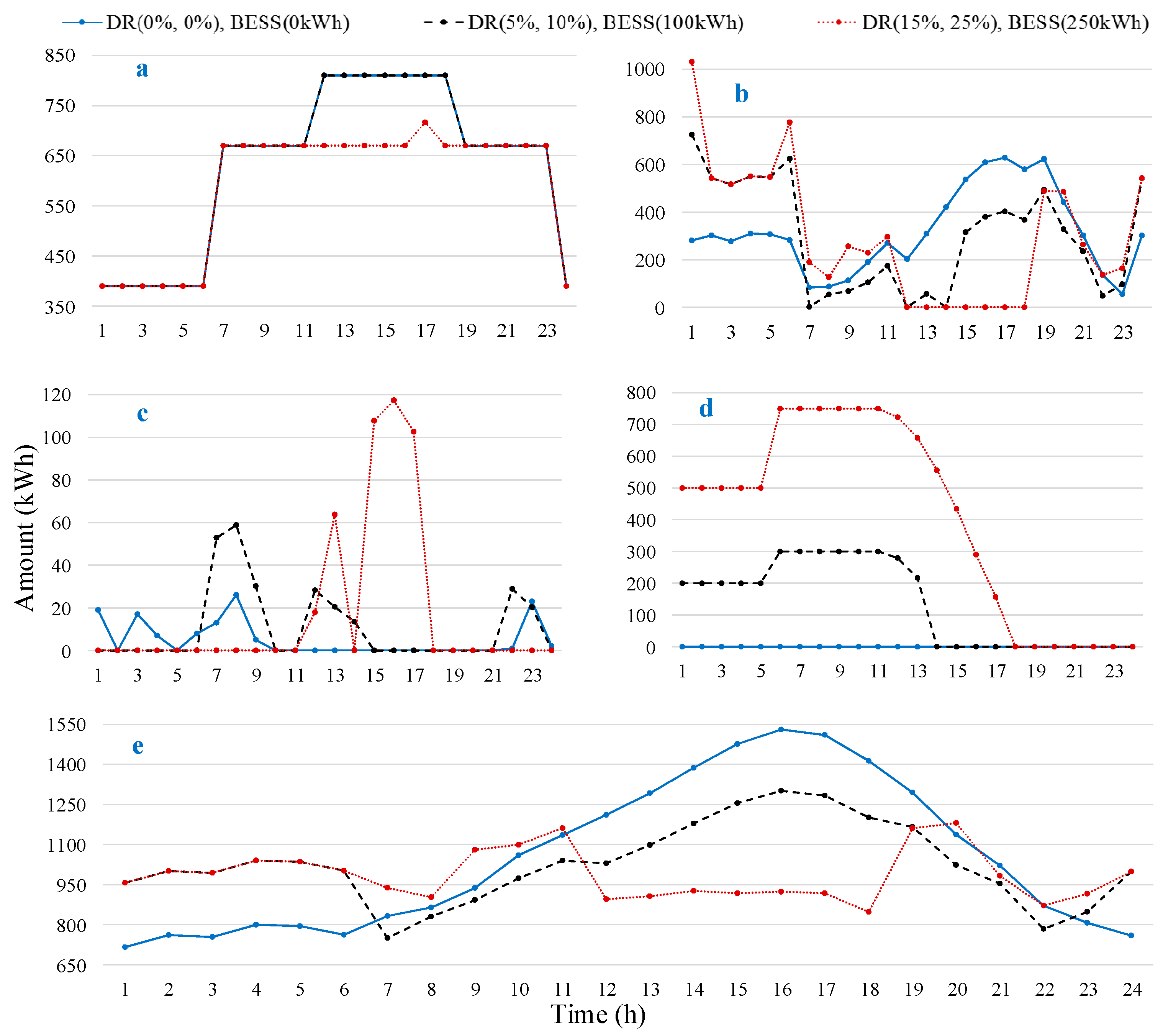
In this section, DR intensity and BESS size are varied simultaneously and three different cases are simulated. Similar to Section 4.2, both price-based DR and incentive-based DR are considered, and are varied from 0% to 25% and 0% to 15%, respectively. Similar to Section 4.3, BESS size is varied from 0 kWh to 250 kWh in each microgrid of the network. The incentive-based DR intensity, price-based DR intensity, and BESS sizes are set to 0%, 0%, 0 kWh for the first case; 5%, 10%, 100 kWh for the second case; and 15%, 25%, 250 kWh for the third case. The impact of these variations on generation pattern of CDGs, power transfer among microgrids of the network, power trading with the utility grid, SOC profile of BESS units, and load profile of the microgrid network is analyzed. Similar to the previous two sections, the accumulated results of all the microgrids are shown in Figure 8.
The generation pattern of CDGs follows the market price signals for the first two cases and is similar to corresponding cases of previous sections. However, in the third case, generation of CDGs is reduced during peak hours as compared to the first two cases, as shown in Figure 8a. This reduction is due to the presence of a higher amount of controllable loads (shiftable and curtailable). Due to both shifting and curtailment of loads during peak hours, load requirement has reduced. In addition, selling to the utility grid is not economical during peak hours due to lower selling price as compared to the generation cost. In this case, the external trading profile of the network is similar to that of Section 4.2, as shown in Figure 8b. However, the magnitude of external trading during initial off-peak intervals has increased from the first case to the last case, as expected. This increase is due to buying more power from the utility grid for charging BESS units. Similarly, the reduction of external trading during peak hours is also more prominent as compared to the results of Section 4.2. This reduction is due to the presence of fully charged BESS units along with higher DR intensity in each microgrid.
The SOC profile of BESS units is in accordance with the external trading profile of the network, as shown in Figure 8d. More electricity is bought during the initial off-peak price intervals and BESS units are charged. The BESS units are discharged during peak-price intervals to avoid buying from the utility grid. The load profile of the microgrid network is identical to that of Section 4.2, as shown in Figure 8e. This is due to the effect of DR programs only on the load profile of microgrids. Similar to previous sections, internal trading does not follow any specific pattern due to the variation of load profile with change in DR intensity, as shown in Figure 8c.
The effect of both DR intensity and BESS size on the net power trading/transfer and daily operation cost of the microgrid network is summarized in Table 7. The net power trading with the utility grid (external power trading) has decreased when both BESS size and DR intensity are increased. This is due to the larger amount of controllable loads in the network as compared to the BESS sizes. The daily operation cost is reduced when both DR intensity and BESS size are increased. The decreasing slope of operation cost is steeper as compared to the previous two sections, due to the presence of both DR programs and BESS units. Similar to the DR-only case, the net internal trading does not follow a specific trend due to the load profile change of individual microgrids with the change in DR intensity.
5. Conclusions
The impact of DR program intensity and BESS size on the operation of networked microgrids is analyzed in this paper. Both price-based DR programs and incentive-based DR programs are considered and BESS size is varied in each microgrid for three different cases. In all the cases, the operation cost of the microgrid network, internal power transfer, external power trading, load profile of the network, and SOC profile of BESS units are analyzed. The prevailing uncertainties in the microgrids, i.e., loads, renewables, and market price signals, are realized via a robust optimization method and a worst-case scenario is considered. Robust optimization can provide immunity against the worst-case scenario if the uncertainties lie within the specified bounds. Simulation results have shown that with an increase in price-based DR intensity, external trading remains the same due to only shifting loads from peak price hours to non-peak price hours. However, external trading has reduced with the increase in incentive-based DR programs, due to curtailment of loads during peak hours. Finally, external trading has reduced with the increase in BESS size due to the buying of electricity during off-peak hours and selling back during peak hours. The operation cost of the network has been reduced for increases in both DR intensity and BESS size. Therefore, it can be concluded that an increase in BESS size is favorable if an increase in external trading and a decrease in internal power transfer are required. On the other hand, an increase in incentive-based DR is favorable if decreases in both internal power transfer and external power trading are required. Finally, price-based DR is favorable for reducing operation costs and has no systematic effect on internal power transfer.
Acknowledgments
This work was supported by the Power Generation & Electricity Delivery Core Technology Program of the Korea Institute of Energy Technology Evaluation and Planning (KETEP), which granted financial assistance from the Ministry of Trade, Industry & Energy, Republic of Korea (No. 20141020402350).
Author Contributions
A. H conceived and designed the experiments; V.-H. B. performed the experiments and analyzed the data; H.-M. K. revised and analyzed the results; A. H. wrote the paper.
Conflicts of Interest
The authors declare no conflict of interest.
Nomenclature
| Identifiers and Binary Variables | |
| Index of time, running from 1 to . | |
| Index of microgrids, running from 1 to and 1 to , respectively. | |
| Index of dispatchable generators, running from 1 to . | |
| Commitment status identifier of dispatchable generator of at . | |
| Start-up and shut-down identifiers of dispatchable generator of at . | |
| , | Identifier for charging and discharging of BESS in . |
| Identifier for load shifting allowance in . | |
| Variables and Constants | |
| Generation cost of dispatchable unit of. | |
| Amount of power generated by dispatchable unit of. | |
| , | Incentive for load curtailment and amount of load curtailed in . |
| Start-up cost of dispatchable unit of. | |
| Shut-down cost of dispatchable unit of. | |
| , | Price for buying and selling power from the utility grid. |
| , | Amount of power bought from and sold to the utility grid by. |
| Amount of fixed and adjusted electric load of . | |
| Amount of curtailable and shiftable electric load of . | |
| Amount of load shifted from in microgrid m. | |
| , | Amount of electrical energy charged/discharged to/from BESS of . |
| , | Amount of power sent by/received from. |
| Forecasted power of RDG unit of. | |
| Capacity of line connecting mth MG with utility grid and nth MG, respectively. | |
| (t) | Amount of power received by mth MG from nth MG at. |
| (t) | Amount of power sent by mth MG to nth MG at |
| , | Surplus and deficit amount of power in. |
| Capacity and SOC of BEES in | |
| Charging and discharging loss of BESS in | |
| , | Maximum load allowed to shift to interval t and allowed to shift from t in MG m. |
| , | Bounded load and associated uncertainty bound in MG m at t |
| Bounded RDG output power and associated uncertainty bound in | |
| , | Upper and lower bounds of load in. |
| , | Upper and lower bounds of RDG output power in. |
| Scaled deviations for load of. | |
| Scaled deviations for WT power output of. | |
| , | Budget of uncertainty and uncertainty adjustment factor of. |
| , | Dual variables for load and RDG unit of. |
| , | Bounded buying price and associated uncertainty bound in at t |
| , | Bounded selling price and associated uncertainty bound in |
| , | Upper and lower bounds of buying price. |
| , | Upper and lower bounds of selling price. |
| Dual variables for buying price at . | |
| Dual variables for selling price at. | |
| , | Budget of uncertainty for buying and selling price. |
References
- Kim, H.M.; Lim, Y.; Kinoshita, T. An intelligent multiagent system for autonomous microgrid operation. Energies 2012, 5, 3347–3362. [Google Scholar] [CrossRef]
- Nguyen, D.T.; Le, L.B. Optimal energy management for cooperative microgrids with renewable energy resources. In Proceedings of the IEEE International Conference on Smart Grid Communications (Smart Grid Comm), Vancouver, BC, Canada, 21–24 October 2013; pp. 678–683. [Google Scholar]
- Farzan, F.; Vaghefi, S.A.; Mahani, K.; Jafari, M.A.; Gong, J. Operational planning for multi-building portfolio in an uncertain energy market. Energy Build. 2015, 103, 271–283. [Google Scholar] [CrossRef]
- Zhang, Y.; Gatsis, N.; Giannakis, G.B. Robust energy management for microgrids with high-penetration renewables. IEEE Trans. Sustain. Energy 2013, 4, 944–953. [Google Scholar] [CrossRef]
- Battistelli, C.; Baringo, L.; Conejo, A.J. Optimal energy management of small electric energy systems including V2G facilities and renewable energy sources. Electr. Power Syst. Res. 2012, 92, 50–59. [Google Scholar] [CrossRef]
- Hussain, A.; Bui, V.H.; Kim, H.M.; Im, Y.H.; Lee, J.Y. Optimal operation of tri-generation microgrids considering demand uncertainties. Int. J. Smart Home 2016, 10, 131–144. [Google Scholar] [CrossRef]
- Jian, L.; Xue, H.; Xu, G.; Zhu, X.; Zhao, D.; Shao, Z.Y. Regulated charging of plug-in hybrid electric vehicles for minimizing load variance in household smart microgrid. IEEE Trans. Ind. Electr. 2013, 60, 3218–3226. [Google Scholar] [CrossRef]
- Hussain, A.; Bui, V.H.; Kim, H.M. Robust optimization-based scheduling of multi-microgrids considering uncertainties. Energies 2016, 9, 278–298. [Google Scholar] [CrossRef]
- Xiang, Y.; Liu, J.; Liu, Y. Robust energy management of microgrid with uncertain renewable generation and load. IEEE Trans. Smart Grid 2016, 7, 1034–1043. [Google Scholar] [CrossRef]
- Hussain, A.; Bui, V.H.; Kim, H.M. Impact quantification of demand response uncertainty on unit commitment of microgrids. In Proceedings of the IEEE International Conference on Frontiers of Information Technology (FIT), Islamabad, Pakistan, 19–21 December 2016; pp. 274–279. [Google Scholar]
- Kwag, H.G.; Kim, J.O. Reliability modeling of demand response considering uncertainty of customer behavior. Appl. Energy 2014, 122, 24–33. [Google Scholar] [CrossRef]
- Soroudi, A. Possibilistic-scenario model for DG impact assessment on distribution networks in an uncertain environment. IEEE Trans. Power Syst. 2012, 27, 1283–1293. [Google Scholar] [CrossRef]
- Bertsimas, D.; Sim, M. The price of robustness. Oper. Res. 2004, 52, 35–53. [Google Scholar] [CrossRef]
- Hussain, A.; Bui, V.H.; Kim, H.M. Fuzzy logic-based operation of battery energy storage systems (BESSs) for enhancing the resiliency of hybrid microgrids. Energies 2017, 10, 271–290. [Google Scholar] [CrossRef]
- Hussain, A.; Arif, S.M.; Aslam, M.; Shah, S.D.A. Optimal siting and sizing of tri-generation equipment for developing an autonomous community microgrid considering uncertainties. Sustain. Cities Soc. 2017, 32, 318–330. [Google Scholar] [CrossRef]
- Hosseinimehr, T.; Ghosh, A.; Shahnia, F. Cooperative control of battery energy storage systems in microgrids. Int. J. Elect. Power Energy Syst. 2017, 87, 109–120. [Google Scholar] [CrossRef]
- Tan, X.; Li, Q.; Wang, H. Advances and trends of energy storage technology in Microgrid. Int. J. Elect. Power Energy Syst. 2013, 44, 179–191. [Google Scholar] [CrossRef]
- Kerdphol, T.; Qudaih, Y.; Mitani, Y. Optimum battery energy storage system using PSO considering dynamic demand response for microgrids. Int. J. Elect. Power Energy Syst. 2016, 83, 58–66. [Google Scholar] [CrossRef]
- Chen, S.X.; Gooi, H.B.; Wang, M. Sizing of energy storage for microgrids. IEEE Trans. Smart Grid 2012, 3, 142–151. [Google Scholar] [CrossRef]
- Zhou, N.; Liu, N.; Zhang, J.; Lei, J. Multi-objective optimal sizing for battery storage of PV-based microgrid with demand response. Energies 2016, 9, 591. [Google Scholar] [CrossRef]
- Khatibzadeh, A.; Besmi, M.; Mahabadi, A.; Reza Haghifam, M. Multi-agent-based controller for voltage enhancement in AC/DC hybrid microgrid using energy storages. Energies 2017, 10, 169. [Google Scholar] [CrossRef]
- Nguyen, T.A.; Crow, M.L. Stochastic optimization of renewable-based microgrid operation incorporating battery operating cost. IEEE Trans. Power Syst. 2016, 31, 2289–2296. [Google Scholar] [CrossRef]
- Mazidi, M.; Zakariazadeh, A.; Jadid, S.; Siano, P. Integrated scheduling of renewable generation and demand response programs in a microgrid. Energy Convers. Manag. 2014, 86, 1118–1127. [Google Scholar] [CrossRef]
- Nwulu, N.I.; Xia, X. Optimal dispatch for a microgrid incorporating renewables and demand response. Renew. Energy 2017, 101, 16–28. [Google Scholar] [CrossRef]
- Karapetyan, A.; Khonji, M.; Chau, C.K.; Elbassioni, K.; Zeineldin, H. Efficient algorithm for scalable event-based demand response management in microgrids. IEEE Trans. Smart Grid 2017. [Google Scholar] [CrossRef]
- Pourmousavi, S.A.; Nehrir, M.H. Real-time central demand response for primary frequency regulation in microgrids. IEEE Trans. Smart Grid 2012, 3, 1988–1996. [Google Scholar] [CrossRef]
- Cha, H.J.; Won, D.J.; Kim, S.H.; Chung, I.Y.; Han, B.M. Multi-agent system-based microgrid operation strategy for demand response. Energies 2015, 8, 14272–14286. [Google Scholar] [CrossRef]
- Hussain, A.; Bui, V.H.; Lee, B.H.; Kim, H.M. Impact analysis of demand response and energy storage in microgrids. In Proceedings of the Korea Institute of Electrical Engineers, Summer Conference, Pyeongchang-gun, South Korea, 4–6 July 2016; pp. 458–460. [Google Scholar]
- US DoE, Benefits of Demand Response in Electricity Markets and Recommendations for Achieving Them, Report to the US Congress. 2006. Available online: http://eetd.idi.gov.
- Garrett, F.; James, M.; Jesse, M.; Hervé, T. The Economics of Battery Energy Storage. 2015. Available online: http://www.rmi.org/ELECTRICITY_BATTERY_VALUE (accessed on 17 May 2017).
- Bui, V.H.; Hussain, A.; Kim, H.M. A multiagent-based hierarchical energy management strategy for multi-microgrids considering adjustable power and demand response. IEEE Trans. Smart Grid 2016, pp. [Google Scholar] [CrossRef]
- Wang, Y.; Shiwen, M.; Nelms, R.M. On hierarchical power scheduling for the macrogrid and cooperative microgrids. IEEE Trans. Ind. Inf. 2015, 11, 1574–1584. [Google Scholar] [CrossRef]
- Bertsimas, D.; Sim, M. Robust discrete optimization and network flows. Math. Program. 2003, 98, 49–71. [Google Scholar] [CrossRef]
Figure 1.
An overview of different demand response (DR) programs.
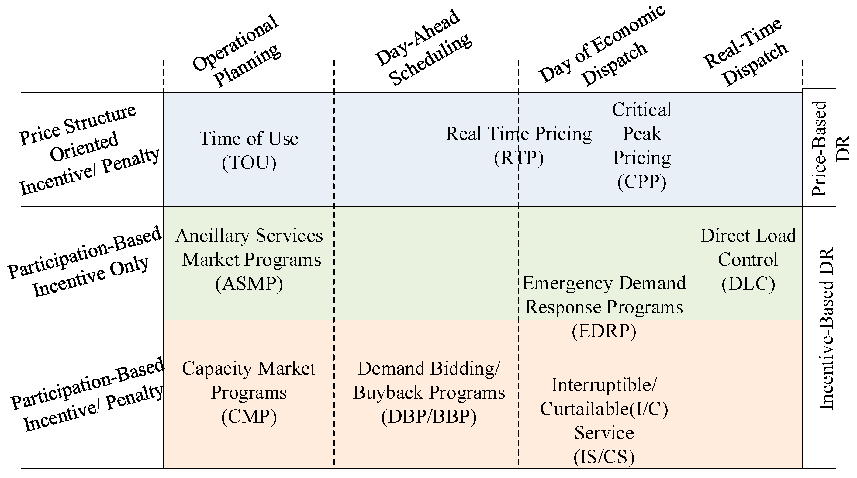
Figure 2.
An overview of the benefits of a battery energy storage system (BESS).

Figure 3.
A typical networked microgrid.

Figure 4.
Real-time market price signals and generation cost of CDGs in each microgrid.

Figure 5.
Input parameters of each microgrid: (a) Forecasted load values; (b) renewable power output.
Figure 5.
Input parameters of each microgrid: (a) Forecasted load values; (b) renewable power output.

Figure 6.
(a) Generation of CDGs; (b) external power trading; (c) internal power transfer; (d) load profile.
Figure 6.
(a) Generation of CDGs; (b) external power trading; (c) internal power transfer; (d) load profile.

Figure 7.
(a) Generation of CDGs; (b) external power trading; (c) internal power transfer; (d) BESS SOC.
Figure 7.
(a) Generation of CDGs; (b) external power trading; (c) internal power transfer; (d) BESS SOC.
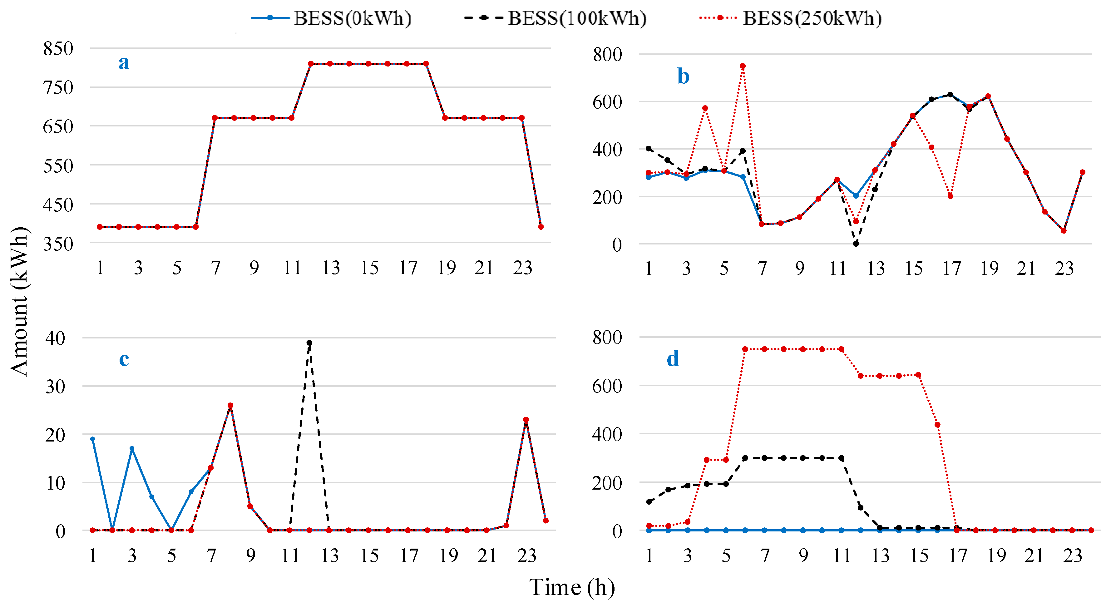
Figure 8.
(a) Generation of CDGs; (b) external power trading; (c) internal power transfer; (d) BESS SOC; (e) load profile of microgrid network.
Figure 8.
(a) Generation of CDGs; (b) external power trading; (c) internal power transfer; (d) BESS SOC; (e) load profile of microgrid network.


Table 1.
Summary of available approaches for battery energy storage systems (BESS) and demand response (DR) with uncertainties.
Table 1.
Summary of available approaches for battery energy storage systems (BESS) and demand response (DR) with uncertainties.
| Major Consideration(s) | Optimization Method | Ref. |
|---|---|---|
| Uncertainties in renewable energy sources | Robust optimization | [ 4,5] |
| Uncertainties in forecasted load values | [ 6] | |
| Using electrical vehicles | [ 7] | |
| Uncertainties in both renewables and forecasted loads | Robust optimization | [ 8,9] |
| Uncertainties in demand response | [ 10] | |
| Multi-stage modeling | [ 11] | |
| Impact of distributed generators on uncertainty | Stochastic optimization | [ 12] |
| Operation of BESS for improving resilience | Fuzzy logic | [ 14] |
| Optimal siting and sizing of BESS | Particle swarm optimization | [ 18] |
| Cost-benefit analysis | [ 19] | |
| Multi-objective model for maximum photovoltaic consumptive rate and net profit | Non-dominated sorting genetic algorithm II | [ 20] |
| Modeling for using BESS as a dispatchable generators | Stochastic optimization | [ 22] |
| DR for compensating forecasting errors | [ 23] | |
| Incentive-based DR programs | Sensitivity analysis | [ 24] |
| Event-based DR management in microgrids | A greedy approach | [ 25] |
| DR for frequency regulation and load minimization | Multi-agent system | [ 26] |
| Impact of DR on industrial loads | [ 27] |
Table 2.
Demand response intensity and BESS capacity range in each microgrid.
| Parameter | Price-Based DR (%) | Incentive-Based DR (%) | BESS Capacity (kW) | ||||||
|---|---|---|---|---|---|---|---|---|---|
| MG1 | MG2 | MG3 | MG1 | MG2 | MG3 | MG1 | MG2 | MG3 | |
| Minimum | 0 | 0 | 0 | 0 | 0 | 0 | 0 | 0 | 0 |
| Maximum | 25 | 25 | 25 | 15 | 15 | 15 | 250 | 250 | 250 |
Table 3.
Uncertainty bounds for uncertain parameters in each microgrid.
| Parameter | Renewable Power (%) | Load (%) | Market Price Signals (%) | |||||
|---|---|---|---|---|---|---|---|---|
| MG1 | MG2 | MG3 | MG1 | MG2 | MG3 | Buying price | Selling Price | |
| Upper bound | 20 | 20 | 20 | 10 | 10 | 10 | 15 | 15 |
| Lower bound | –20 | –20 | –20 | –10 | –10 | –10 | –15 | –15 |
Table 4.
Parameters related to controllable distributed generators (CDGs) and line capacities of the network.
Table 4.
Parameters related to controllable distributed generators (CDGs) and line capacities of the network.
| Parameter | CDG Generation (kW) | Line Capacity (kW) | |||||||
|---|---|---|---|---|---|---|---|---|---|
| MG1 | MG2 | MG3 | MG1 ↔ MG2 | MG1 ↔ MG3 | MG2 ↔ MG3 | MG1 ↔ UG | MG2 ↔ UG | MG3 ↔ UG | |
| Minimum | 0 | 170 | 0 | 0 | 0 | 0 | 0 | 0 | 0 |
| Maximum | 220 | 310 | 280 | 400 | 400 | 400 | 600 | 600 | 600 |
Table 5.
Effect of DR intensity on power transfer and operation cost.
| DR Intensity (%) | Internal Power Transfer (kW) | External Power Trading (kW) | Operation Cost (KRW) | Decrease (%) | |
|---|---|---|---|---|---|
| Price-Based | Incentive-Based | ||||
| 0 | 0 | 121 | 7648 | 2,279,910.0000 | 0.00 |
| 0.05 | 0.03 | 172.8 | 7353.43 | 2,240,424.0000 | 1.73 |
| 0.1 | 0.06 | 199.8 | 7157.05 | 2,209,872.0000 | 3.07 |
| 0.15 | 0.09 | 0.04 | 6900.31 | 2,201,409.5600 | 3.44 |
| 0.2 | 0.12 | 0 | 6675.3 | 2,195,181.2800 | 3.72 |
| 0.25 | 0.15 | 45.65 | 6426.4 | 2,192,273.0000 | 3.84 |
Table 6.
Effect of BESS size on power transfer and operation cost.
| BESS Size (kW) | Internal Power Transfer (kW) | External Power Trading (kW) | Operation Cost (KRW) | Decrease (%) |
|---|---|---|---|---|
| 0 | 121 | 7648 | 2,279,910.0000 | 0.00 |
| 50 | 121 | 7654.0604 | 2,273,044.8320 | 0.30 |
| 100 | 109 | 7660.1228 | 2,266,179.8240 | 0.60 |
| 150 | 114.003 | 7667.33799 | 2,259,464.7887 | 0.90 |
| 200 | 73.003 | 7672.246 | 2,252,449.6800 | 1.20 |
| 250 | 70.003 | 7678.471 | 2,245,605.9300 | 1.50 |
Table 7.
Effect of DR intensity & BESS size on power transfer and operation cost.
| DR Intensity (%) | BESS Size (kW) | Internal Power Transfer (kW) | External Power Trading (kW) | Operation Cost (KRW) | Decrease (%) | |
|---|---|---|---|---|---|---|
| Price-Based | Incentive-Based | |||||
| 0 | 0 | 0 | 121 | 7648 | 2,279,910.0000 | 0.00 |
| 0.05 | 0.03 | 50 | 179.84 | 7359.49 | 2,233,558.8000 | 2.03 |
| 0.1 | 0.06 | 100 | 253.551 | 7169.9853 | 2,196,247.4590 | 3.67 |
| 0.15 | 0.09 | 150 | 130.023 | 6919.7064 | 2,180,947.5760 | 4.34 |
| 0.2 | 0.12 | 200 | 56.535 | 6754.116 | 2,168,375.8000 | 4.89 |
| 0.25 | 0.15 | 250 | 409.65 | 7138.906 | 2,166,133.8800 | 4.99 |
© 2017 by the authors. Licensee MDPI, Basel, Switzerland. This article is an open access article distributed under the terms and conditions of the Creative Commons Attribution (CC BY) license (http://creativecommons.org/licenses/by/4.0/).
Share and Cite
MDPI and ACS Style
Hussain, A.; Bui, V.-H.; Kim, H.-M. Impact Analysis of Demand Response Intensity and Energy Storage Size on Operation of Networked Microgrids. Energies 2017, 10, 882. https://doi.org/10.3390/en10070882
AMA Style
Hussain A, Bui V-H, Kim H-M. Impact Analysis of Demand Response Intensity and Energy Storage Size on Operation of Networked Microgrids. Energies. 2017; 10(7):882. https://doi.org/10.3390/en10070882
Chicago/Turabian StyleHussain, Akhtar, Van-Hai Bui, and Hak-Man Kim. 2017. "Impact Analysis of Demand Response Intensity and Energy Storage Size on Operation of Networked Microgrids" Energies 10, no. 7: 882. https://doi.org/10.3390/en10070882
Note that from the first issue of 2016, this journal uses article numbers instead of page numbers. See further details here.