Combined Heat and Power Dispatch Considering Heat Storage of Both Buildings and Pipelines in District Heating System for Wind Power Integration


Department of Electrical Engineering, Dalian University of Technology, Dalian 116024, China
*
Author to whom correspondence should be addressed.
Energies 2017, 10(7), 893; https://doi.org/10.3390/en10070893
Submission received: 11 May 2017
/
Revised: 8 June 2017
/
Accepted: 28 June 2017
/
Published: 30 June 2017
(This article belongs to the Section F: Electrical Engineering)
Abstract
:The strong coupling between electric power and heat supply highly restricts the electric power generation range of combined heat and power (CHP) units during heating seasons. This makes the system operational flexibility very low, which leads to heavy wind power curtailment, especially in the region with a high percentage of CHP units and abundant wind power energy such as northeastern China. The heat storage capacity of pipelines and buildings of the district heating system (DHS), which already exist in the urban infrastructures, can be exploited to realize the power and heat decoupling without any additional investment. We formulate a combined heat and power dispatch model considering both the pipelines’ dynamic thermal performance (PDTP) and the buildings’ thermal inertia (BTI), abbreviated as the CPB-CHPD model, emphasizing the coordinating operation between the electric power and district heating systems to break the strong coupling without impacting end users’ heat supply quality. Simulation results demonstrate that the proposed CPB-CHPD model has much better synergic benefits than the model considering only PDTP or BTI on wind power integration and total operation cost savings.
1. Introduction
The installed capacity of wind turbines has been increasing recently in China [1], involving much uncertainty for the electric power system (EPS), which puts forward higher requirements for the system operational flexibility. The electric power generation range of the combined heat and power (CHP) units is severely restricted by the heat loads due to the power and heat coupling during heating seasons. The CHP units have to remain on certain constrained electric power output to meet the heat loads’ demand, leaving little room for wind power integration during the wind power on-peak hours with low electric loads, but high heat loads. This makes the system operational flexibility become low, which results in heavy wind power curtailment, especially in the cold region with a high percentage of CHP units and abundant wind power energy, such as northeastern China. [1]. Therefore, breaking the power and heat coupling of CHP units to improve the system operational flexibility is crucial to reduce wind power curtailment.
It is an effective way to realize the power and heat decoupling by the optimal operation of multi-energy systems, which coordinate at least two different energy systems, such as electric power, heating, cooling or gas system, etc., with many advantages of lower operation cost, higher renewable energy integration and more reliable energy supply. Installing heat storage facilities [2,3,4,5,6] and introducing electricity-heat conversion devices [7,8,9,10,11] in CHP plants can coordinate the electric power and heat energy to utilize the flexibility of the heating system. Moradi et al. [12,13] introduced a novel approach for optimal management of multi-energy including heating, cooling and power in residential buildings to achieve high energy efficiency, low greenhouse gas emission and low generation cost. Ye et al. [14] proposed an integrated natural gas, heat and power dispatch model considering wind power and a power-to-gas unit to reduce wind power curtailment, fuel cost and CO emissions.
The above approaches are greatly restricted by their high capital investment for introducing some other facilities, such as heat storage tanks, electric boilers, heat pumps, chillers, etc. Additionally, they abstract the pipeline network and heating buildings of the district heating system (DHS) into a single static heat load node model without considering their internal thermal characteristics. The urban DHS infrastructures already exist, including many insulated pipelines with a large capacity of internal heat water and a huge area of heating buildings with significant insulated envelope structures, which have plenty of heat storage capacity [15,16,17]. The DHS heat storage can be utilized to break the power and heat coupling without any additional investment in the scope of the combined heat and power system. Recently, several studies have focused on exploiting the DHS internal thermal characteristics including the pipelines’ dynamic thermal performance (PDTP) and the buildings’ thermal inertia (BTI) to improve the system operational flexibility.
Considering only PDTP, the thermal performance mainly refers to two factors including the water heat loss of pipelines and the water temperature time delays from heat sources to heat loads. The pipeline model was built considering heat loss [18,19,20] in the optimal supply and distribution of electric power and heat energy. Zhao et al. [21] studied the optimal operation of a CHP-type district heating system considering time delays in the distribution network. To further account for the effect of the pipelines’ heat storage, the two factors were both considered [16], which established the pipeline model based on the node method [22] to describe the temperature dynamic profiles along the pipelines. Fu et al. [23] described the thermal performance by AMRA time series considering the DHS as a black box.
For considering only BTI, the potential of residential buildings as thermal energy storage in the DHS was studied through pilot tests [24,25,26]. Satyavada et al. [27,28] proposed an integrated control-oriented approach to describe the thermal characteristics of the heating, ventilating and air conditioning equipment in the buildings with modular models effectively. Yang et al. [29] utilized thermal energy storage and distributed electric heat pumps considering BTI to improve wind power integration. Wu et al. [30] proposed a novel day-ahead scheduling method and strategy by use of the indoor temperature adjustable region and BTI to reduce wind power curtailment. Pan et al. [31] proposed a modified feasible region method to give a new formulation of the DHS models similar to conventional power plants. Jin et al. [17] developed a building-based virtual energy storage system model to participate in the economic dispatch of the hybrid energy microgrid.
Coordinating the operation of both PDTP and BTI should be better than considering only one of them, since the district heating pipelines and buildings are connected together, which constitute the heat transmission, distribution and consumption sections of the DHS. The approaches involving both pipeline and building models are rarely studied. Li et al. [32] set up a simulation model of a single back pressure CHP plant-based district heating system with Ebsilon software, which analyzed the system performance by the simulation method. The economic operation of a district electricity and heating system was studied [33], which focused on the two systems’ disturbance interaction effect on the system security. Further, they did not consider the coordinating effect of both PDTP and BTI in the optimal operation of EPS and DHS for wind power integration.
To bridge these gaps, this paper proposes a combined heat and power dispatch model considering both PDTP and BTI simultaneously (CPB-CHPD model) to reduce wind power curtailment and total operation cost, which meets the electric load and heat load demands, as well as satisfies the EPS and DHS constraints. This approach exploits the coordinating effect of both PDTP and BTI to break the strong linkage of power and heat supply of CHP units more effectively. The benefits of only PDTP, only BTI and both of them are separately evaluated in terms of improving wind power integration and reducing total operation cost to demonstrate the synergic benefits of both PDTP and BTI.
The main contributions of this paper are summarized as follows:
- A novel CPB-CHPD model is proposed with special emphasis on the coordinating operation of both PDTP and BTI aiming at breaking the power and heat coupling to significantly improve the system operational flexibility without any additional investment.
- A physical model of the DHS is proposed. The pipeline model is built considering heat loss, temperature time delays and network topology characteristics in terms of single and network level. The building model is formulated based on buildings’ thermal equilibrium considering building characteristics’ diversity and outdoor temperature variation.
- The synergic benefits of both PDTP and BTI on reducing wind power curtailment and total operation cost are evaluated, which are better than considering only one or neither of them.
This paper is organized as follows. In Section 2, the DHS is modeled regarding both PDTP and BTI. Then, the CPB-CHPD is formulated in Section 3. In Section 4, simulation cases are carried out to compare the four dispatch models (including considering both PDTP and BTI, or only one of them, or neither) to demonstrate the synergic effects of the CPB-CHPD model. Finally, the conclusions are given in Section 5.
2. System Model of the DHS
The typical DHS is composed of a heat source mainly referring to the high efficiency coal-fired CHP unit, a district heating pipeline network and many heat loads, which are usually space heating for the residential buildings especially in cold northeastern China.
2.1. Heat Sources
2.1.1. Electric and Heat Power Characteristics
The electric and heat power characteristics of both extraction condensing and back pressure turbine CHP units are shown in Figure 1. The operation points of the two kinds of CHP units are kept respectively inside the polygon region ABCD and on the line segment BC [34].
The electric and heat power limits of the extraction condensing turbine CHP units are described in Equations (1) and (2).
where the subscript i, the subscript t and the subscript chp denote the -th CHP unit, the -th dispatch period and the relevant variables of the CHP unit, respectively, and are the electric and heat power output (), and are the maximum and minimum electric power output in condensing operation condition (), is the maximum heat power output (), and are the curve slope of electric power to heat power in the extraction operation condition, refers to back pressure operation condition, is the electric power value at the intersection between the extension of back pressure curve and the electric power axis () and N is the index set of dispatch periods.
The back pressure turbine CHP units can be regarded as special operation conditions of the extraction condensing units when but . That is to say, the electric and heat power limits of the back pressure units can be described in Equation (3).
2.1.2. Operation Cost
The operation cost of the CHP unit is expressed as a quadratic function of their electric and heat power output [29]:
where is the operation cost function, is the coal consumption function, , and are the coal consumption coefficients (, , ), is the price of the standard coal, in this paper, and is the index set of CHP units.
2.2. District Heating Pipelines Network
Due to the lack of control devices at the end users in China, most of the DHSs are operated with constant flow and variable temperatures [31]. It is assumed that this operation mode is also utilized in this paper, where the mass flow rate is always constant, and the hydraulic conditions always keep stable. Then, we can focus on studying the thermodynamic model of the pipeline network with eliminating the nonlinear hydraulic model to simplify the solving [31]. This impact on the combined heat and power dispatch results is within acceptable limits [35]. In this paper, the PDTP is modeled at two levels, which are the single pipeline level and the pipeline network level.
2.2.1. Single Pipeline Level
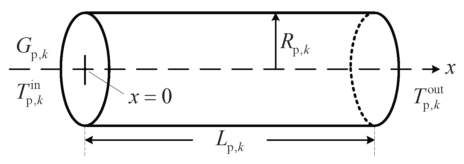
The dynamic characteristics on a single pipeline level mainly are reflected in thermal conduction along the pipeline. Figure 2 shows the general structure of a single pipeline [36].
The thermal conduction in each pipeline, including heat loss and temperature time delays, can be modeled by a partial differential equation [16,36] as follows:
where the subscript k and the subscript denote the -th pipeline and the relevant variables of the pipeline, is the water temperature at a length of x from the inlet inside the pipeline (), is the soil temperature outside the pipeline (), is the mass flow rate (), is the specific heat capacity of the hot water (), is the density of the hot water (), and are the radius and length of the pipeline (), is the thermal loss coefficient () and is the index set of pipelines.
The solution of Equation (5) can be obtained [36,37] as follows:
where and are the water temperature at the inlet and outlet of the pipeline (), and the delay time represents water flowing time from the inlet to the outlet of the pipeline, which can be comparable with one or several dispatch periods of the EPS. Since the mass flow rate is constant in this paper, is defined by:
The subscript in Equation (6) is required to be an integer. In order to utilize Equations (6) and (7) in the discrete dispatch model, we rewrite Equation (6) as Equation (8).
where is the multiples of the continuous delay time to the duration of the discrete dispatch period , which is:
Though this approach will lose some accuracy, it can still describe the PDTP adequately with the advantage of reducing the solving complexity of the combined dispatch model. Additionally, the shorter is, the more accurate the approach is. It requires some initial temperatures of a pipeline (i.e., temperatures before the first dispatch period, which can be known from measurement or prediction) to accomplish Equation (8) when .
2.2.2. Pipeline Network Level
In the district heating pipeline network, heat energy is carried by the circulating hot water, which is transported from the heat sources to the heat loads.
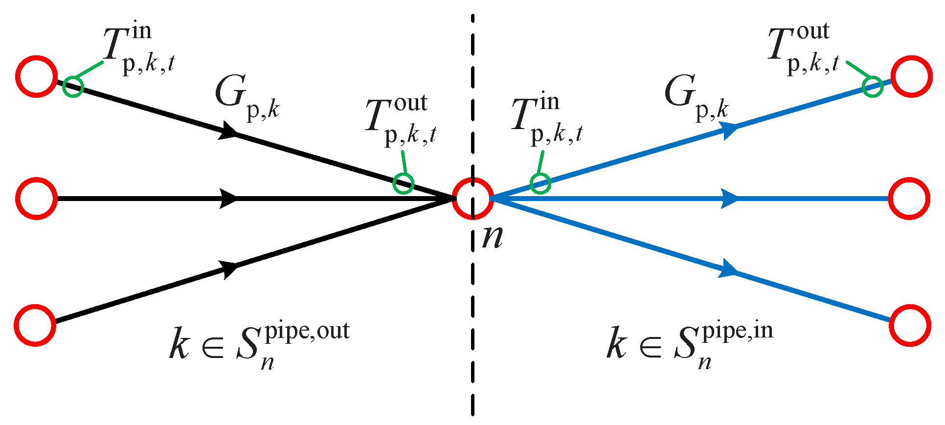
Figure 3 shows the general structure of a node connecting with cross pipelines in the pipelines network [16]. In this paper, we define that the water inflowing side is the inlet of a pipeline, and the water outflowing side is the outlet correspondingly.
The pipeline network topology characteristics are described from four aspects as follows.
- Relationship between heat power and water temperatures:The heat power of the hot water, flowing into the inlet and flowing out of the outlet, of pipeline k at period t is expressed respectively as follows:where and are the heat power flowing into the inlet and flowing out of the outlet of the pipeline ().
- Supply and return water temperature limits:The water temperatures in the water supply and return network should be kept within their limits:where and are the upper and lower limits of water temperatures in the water supply network pipelines (), and are the upper and lower limits of water temperatures in the water return network pipelines () and and are the index sets of pipelines in the water supply and return network.
- Mass flow rates’ continuity and limits:Similar to Kirchhoff’s current law, for each node in the pipeline network, the total mass flow rates of all pipelines connecting to this node is zero:where and are the index sets of pipelines whose inlet and outlet connect to pipeline network node n.The mass flow rates at each period should not exceed their upper or lower limits:where and are the upper and lower limits of the mass flow rate ().
- Node temperature characteristics:According to the energy conservation law, the water temperatures of all pipelines flowing into the same node are mixed at this node, and the water temperatures of all pipelines flowing out of this node are equal to the mixed temperature at this node, as described in Equation (15).where is the mixed temperature at node n in the water supply and return network ().
2.3. Buildings
Since there are many rooms with different structures from each other in a multi-story building and many different buildings in a heating region, it requires a huge calculation to model each room separately, which is almost impossible. In this paper, a lumped model is utilized to abstract a multi-story building or some adjacent buildings with similar characteristics as a large room for simplicity without affecting the thermal inertia performance. The lumped model can describe the BTI adequately for the combined heat and power dispatch model.
2.3.1. Relationship between Indoor Temperatures and Heat Power Supplied
The heat storage of a building is the difference of heat energy supplied and heat energy loss. Considering the winter heating scenario, the thermal equilibrium equation [17] of building j is shown as follows:
- denotes the change rate of the heat energy of the building, as expressed in Equation (17). When the indoor temperature increases, i.e., , the heat energy of the building increases, which means the building heat storage is charged. Oppositely, when the indoor temperature decreases, , the building heat storage is discharged.
- On the right side of Equation (16), the two items in the first parenthesis denote the building total heat energy supplied, where and are the heat power supplied by district heating pipelines and by internal heat gains (such as the effect of indoor lighting, persons, appliances, etc.), respectively. Here, the heat power supplied by internal heat gains is assumed as .
- On the right side of Equation (16), the two items in the second parenthesis denote the building total heat energy loss, where is the sum of the heat power transfer through each side of the building envelope structures including doors, windows, walls, floors, roofs, etc., as expressed in Equation (18). Meanwhile, the solar radiation is appended to the heat power transfer by orientation correction, and the outdoor cold wind speed effect is also appended by its additional correction. is the building heat power loss by cold air infiltration through the windows and doors gaps, as well as cold air intrusion from the opening windows and doors, as expressed in Equation (19); is the index set of buildings.
A concise equation can be obtained [31,38] from Equations (16)–(19) as follows:
where is the building total heat transfer coefficient between the indoor and outdoor air () and is the building equivalent heat storage time coefficient (s), which indicate the building heat energy transfer and storage capacity respectively, as shown in Equations (21) and (22).
In the discrete combined dispatch model, we only focus on the changes of indoor temperatures at the beginning and end of each discrete dispatch period t, neglecting the changes of both the heat power supplied by pipelines to the building and the outdoor temperature within the discrete dispatch period t. With a forward difference approximation on the time derivative, the differential Equation (20) can be converted to a finite difference equation [17], which can describe the coupling relationship of indoor temperatures, heat power supplied and discrete dispatch periods of the building in the discrete combined dispatch model, as expressed in Equation (23). The initial indoor temperatures before the first dispatch period can be known from measurement or prediction.
2.3.2. Indoor Temperatures Limits
In order to ensure the heat supply quality and the thermal comfort, indoor temperatures should be kept within their limits:
where and are the upper and lower limits of indoor temperature (C).
2.4. Interfaces among Heat Sources, Network and Loads
2.4.1. Between Heat Sources and Pipelines Network
At the side of the heat sources, the return water is heated by the CHP unit heat exchanger and then pumped into the supply pipeline network. Heat energy is extracted from the heat sources and distributed to the pipeline network, as expressed in Equations (25) and (26).
where is the heat power through the CHP unit heat exchanger to the pipeline network (), is the efficiency of the CHP unit heat exchanger (0.97), and are the index sets of pipelines in the water supply and return network connecting to pipeline network node n and is the index of pipeline network node connecting to CHP unit i.
2.4.2. Between Pipeline Network and Heat Loads
At the side of the heat loads, i.e., buildings, the supply water releases heat energy to indoor air via heat radiators to maintain the indoor temperatures and then flows into the return pipelines. Heat energy is extracted from the pipeline network and distributed to the heat loads, as expressed in Equation (27).
where is the index of the pipeline network node connecting to building j.
3. Optimization Model of the CPB-CHPD
The CPB-CHPD model including wind farms is formulated in this section. The proposed CPB-CHPD model seeks the optimal dispatch by coordinating the electric power of every power generation unit and the heat power of every heat source aiming at the minimum total operation cost, which includes the penalty cost of wind power spillage, while meeting the electric loads and heat loads demands, as well as satisfying the EPS and DHS constraints.
3.1. Decision Variables
The decision variables in the CPB-CHPD model are composed of two parts, which are the electricity and heat decision variables. The electricity decision variables include the electric power output of CHP units (), condensing power (CON) units () and wind farms (). The heat decision variables include the heat power output of CHP units (), water temperatures at the inlet and outlet of pipelines ( and ), mass flow rates of pipelines (), heat power supplied by pipelines to buildings () and indoor temperatures of buildings ().
3.2. Objective Function
The objective function is the total operation cost consisting of the operation cost of thermal power units and the penalty cost of wind power spillage, as expressed in Equation (28).
- The operation cost of the CHP unit is defined in Equation (4).
- The operation cost of the CON unit is expressed as a quadratic function of its electric power output [16]:where the subscript i and the subscript denote the -th CON unit and the relevant variables of the CON unit, is the operation cost function, is the coal consumption function, is the electric power output (), , and are the coal consumption coefficients (, and ) and is the index set of CON units.
- The penalty cost of the wind farm is proportional to the wind power spillage:where the subscript i and the subscript denote the -th wind farm and the relevant variables of the wind farm, is the penalty cost function, is the wind power output (), is the maximum available wind power (), is the penalty coefficient () and is the index set of wind farms.
3.3. Constraints
The proposed CPB-CHPD model is subject to the EPS constraints and the DHS constraints.
3.3.1. EPS Constraints
The EPS constraints consist of the electric power balance constraints and the units operation constraints, etc.
- Electric power balance constraints:The system total electric power output and total electric loads are equal at each dispatch period:where is the electric load demand () and is the index set of electric loads.
- Units’ operation constraints:
- Generation range constraints:The electric and heat power limits constraints of extraction condensing and back pressure turbine CHP units are defined in Equations (1)–(3).The electric power output of the CON units must be kept within their limits:where and are the maximum and minimum electric power ().The electric power output of the wind farms are limited by the maximum wind power:
- Ramping constraints:
In order to meet the requirements of different cases, some other EPS constraints may be needed, such as the wind power ramping constraints, the spinning reserve constraints, the system operation security constraints, the unit commitment constraints, etc.
3.3.2. DHS Consraints
The DHS constraints consist of the PDTP constraints, the BTI constraints and the interfaces constraints among heat sources, network and loads.
- PDTP constraints:
- BTI constraints:
3.3.3. Interfaces Constraints among Heat Sources, Network and Loads
4. Simulation Cases and Results Analysis
4.1. Simulation System Description
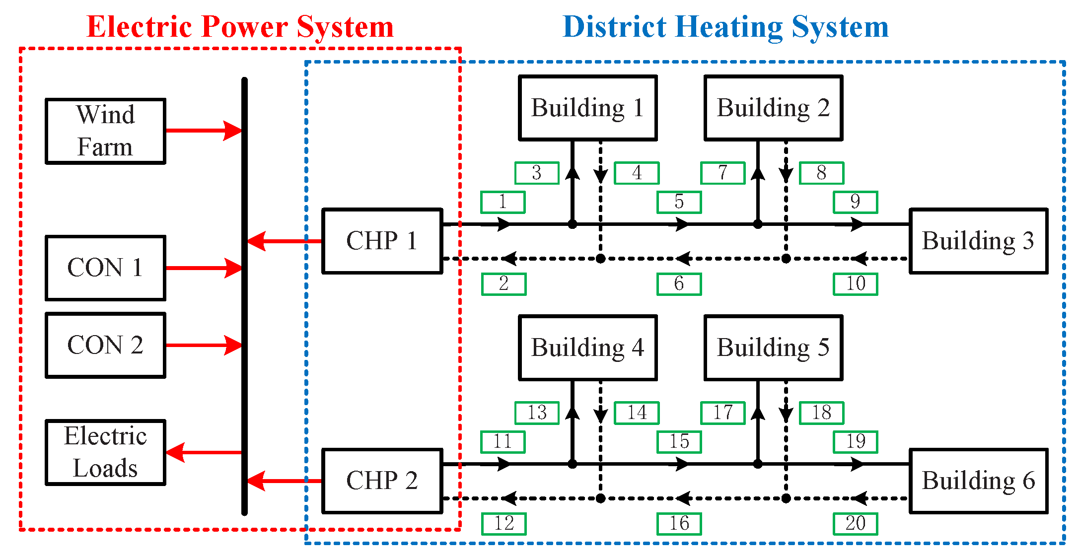
A simulation for the combined heat and power system shown in Figure 4 is carried out to demonstrate the effect of the proposed model, where the EPS consists of two CHP units, two CON units and one wind farm, and the DHS is composed of the two CHP units, twenty pipelines and six buildings. The two CHP units are coupling points between the EPS and DHS. The DHS has sixteen nodes, where Buildings 1–3 are heat supplied via Pipelines 1–10 by CHP 1, and Buildings 4–6 are heat supplied via Pipelines 11–20 by CHP 2.
The parameters of thermal power units, pipelines and buildings are listed in Table 1, Table 2 and Table 3, respectively. The upper and lower limits of water temperatures at every node in the district heating pipelines network are 130 and 50 . The upper and lower limits of the mass flow rates are 3700 and 800 . The standard indoor temperature for space heating is set as 18 , and the thermal comfort indoor temperature ranges of all buildings are set between 18 and 22 . These typical thermal power units are commonly used in northeastern China. The detailed parameters of pipelines and buildings, as well as the DHS operation data are from the typical design data of the standard design specification of heating, ventilation and air conditioning for civil buildings, which is established by the China Academy of Building Research.
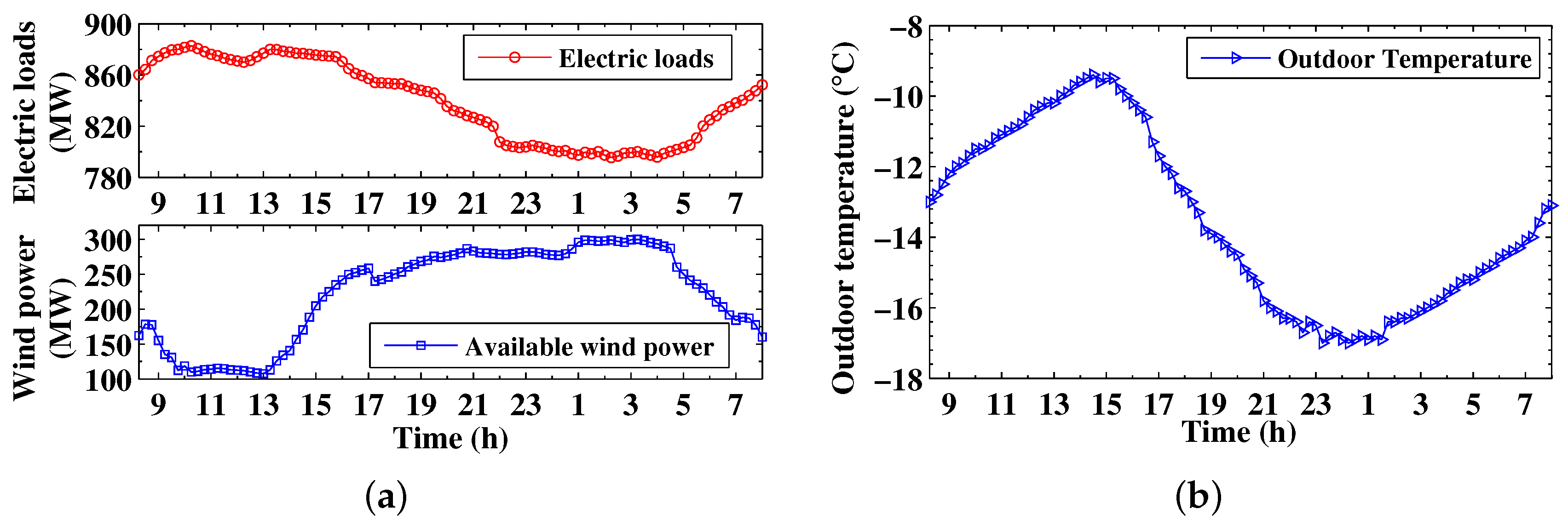
The typical day profiles of the total electric loads and forecast wind power, as well as the outdoor temperature are shown in Figure 5. The forecast wind power has almost the opposite peaks with the total electric loads, which is consistent with the characteristics of the EPS. With some modification, the outdoor temperature is from the historical data of the typical day during the medium heating season in northeastern China when the heat loads demand is high. These weather data were measured by the China Meteorological Administration during the past few years.
All simulation tests are considered for a 15-min operation scheduling over the course of 24 h.
4.2. Cases Settings
Four different dispatch models are given here including the CPB-CHPD, CP-CHPD, CB-CHPD and CED model, where the CPB-CHPD model refers to the model of combined heat and power dispatch considering both PDTP and BTI; the CP-CHPD model refers to the model of combined heat and power dispatch considering only PDTP; and the CB-CHPD refers to only BTI. The CED model refers to the conventional economic dispatch model, which just abstracts the whole of the pipelines and buildings as a simple static heat load node without considering their heat storage capacity. The objective functions of the other three models are the same as the CPB-CHPD model, but they are subject to different constraints listed as follows.
- The differences between the constraints of the CED and CPB-CHPD models are in two aspects. One is that Equations (7)–(15) and (26) should be replaced by Equation (36). The other is that Equations (21)–(24) and (27) should be replaced by Equation (37).where is the standard indoor temperature for space heating () and is the index set of buildings connecting to CHP unit i via pipelines.
The simulation cases are set as follows: (1) Case 1 is utilized to describe the promotion effects on wind power integration and total operation cost savings of the CPB-CHPD model; (2) Case 2 is carried out to compare different results of the four dispatch models (CPB-CHPD, CP-CHPD, CB-CHPD and CED) based on Case 1 to demonstrate the synergic effects by coordinating PDTP and BTI.
4.3. Results Analysis
The electricity tariff is an important factor to the optimal results of the total operation cost. Since the electricity tariff is still regulated at present in China, we do not analyze its effect on the optimal results in this paper. The simulation results of the two cases are given below.
4.3.1. Case 1
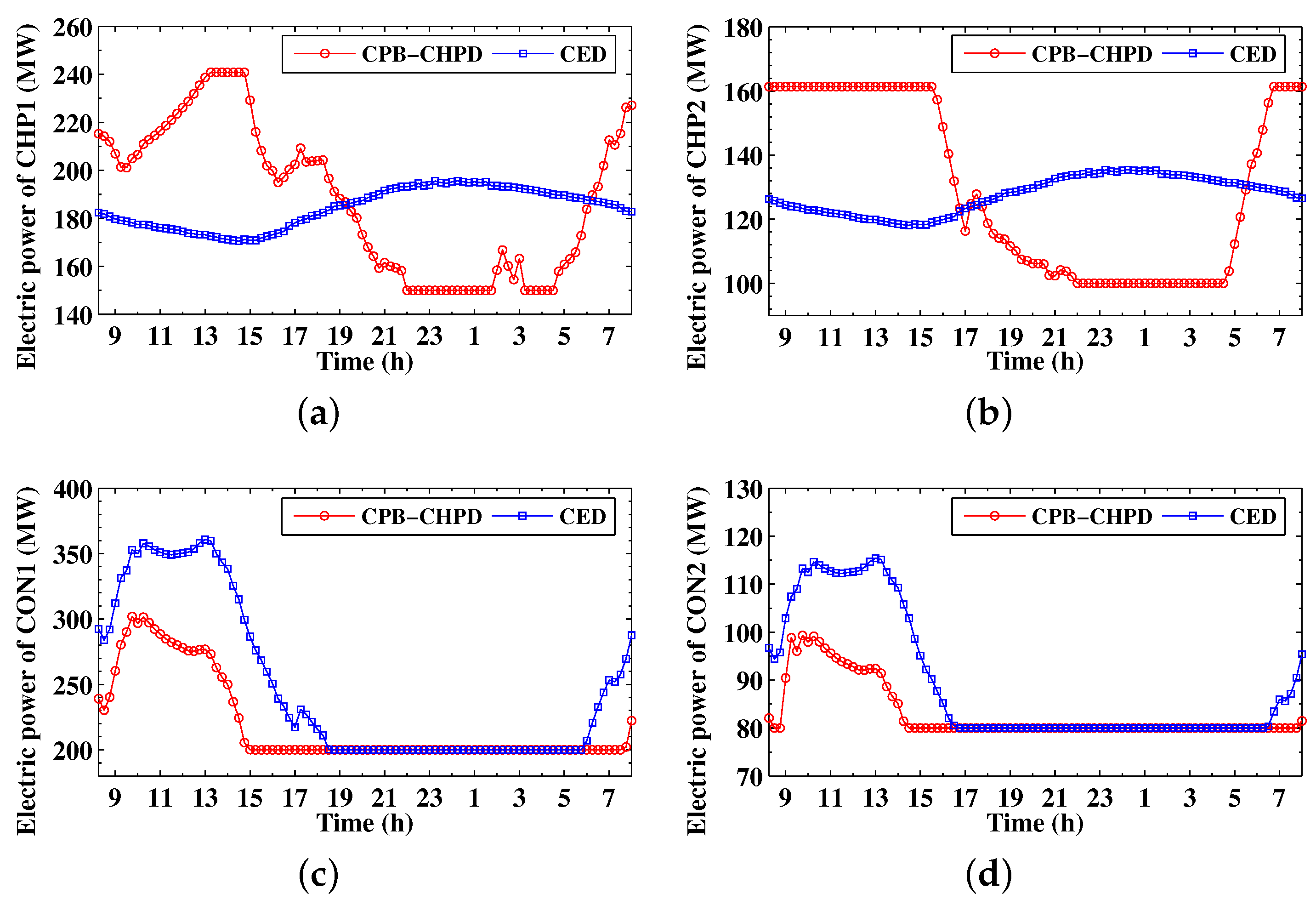
This part is utilized to describe the promotion effects on wind power integration and total operation cost savings of the CPB-CHPD model. The optimization results are shown in Figure 6, Figure 7, Figure 8 and Figure 9, respectively. Owing to the improved system operational flexibility by considering both PDTP and BTI, the total operation cost of the CPB-CHPD model is $521,741, reduced by nearly based on the CED model whose operation cost is $591,929.
For the CED model, the heat power output of the CHP units must be always equal to the heat loads at each period, which are reflected in Figure 7. Comparing Figure 6 and Figure 7 with Figure 8, during the wind power on-peak periods with low electric loads, but high heat load demand, the CHP units have to remain on certain constrained electric and heat power output to meet the high heat load demand because of the power and heat coupling and cannot be reduced any further; meanwhile other CON units have already been dispatched on their minimum technical generation, which results in that there is not enough space for wind power integration. Therefore, heavy wind power spillage occurs due to the inadequate downward spinning reserve.
For the CPB-CHPD model, the heat power output of the CHP units need not equal the heat loads at each period any more, which are required to satisfy the PDTP and BTI constraints instead. As shown in Figure 7, the heat power output of CHP1 and CHP2 is not restricted by the heat loads at each period. However, it is not indicated that they cannot meet the heating requirements of buildings. In contrast, all buildings’ indoor temperatures at each period are kept within the thermal comfort range, as shown in Figure 9.
The average indoor temperatures of all buildings are higher than the standard 18 , which indicates that there will be more heat energy stored in pipelines and buildings, resulting in more heat energy loss simultaneously. This requires the CHP units to produce more heat energy, which increases their operation cost. However, the total operation cost of the CPB-CHPD model decreases due to two reasons. One is that the operation cost of the CON units decreases greatly because their electric power output can be reduced significantly in the CPB-CHPD model, which can be seen in Figure 6c,d. The other is that a large amount of wind power energy can be integrated with saving much of the penalty cost of wind power spillage.
Pipelines and buildings both can be regarded as huge heat storage equipment. Their total heat storage/release capacity, as described in Figure 7, can be represented by the area that is enclosed by the red and blue curves when the red curve is higher/lower than the blue one.
The effect of heat storage in pipelines and buildings is illustrated in Figure 7 and Figure 8 clearly. During the wind power off-peak periods with high electric loads, but low heat load demand, the CHP units can appropriately increase heat power output more than needed. The extra heat energy can be stored in pipelines and buildings, with indoor temperatures rising.
On the contrary, during the wind power on-peak periods with low electric loads, but high heat load demand, the CHP units can appropriately decrease electric and heat power output less than the constrained one of the CED model, which can provide an extra wind power integration space. As shown in Table 4, the CPB-CHPD model can utilize more wind power energy than the CED model by 689.71 MWh accounting for approximate . Due to the lack of heat supply by the CHP units, indoor temperatures drop consequently, but not much, because they can be partly supplemented by heat release from pipelines and buildings. Since the operation status of the DHS changes very slowly, indoor temperatures will not change suddenly and dramatically, which can ensure the heat supply quality.
These simulation results demonstrate that, compared with the CED model, the CPB-CHPD model can break the power and heat coupling of the CHP units greatly, which can improve the system operational flexibility significantly.
4.3.2. Case 2
This part is carried out to compare different results of the four dispatch models (CPB-CHPD, CP-CHPD, CB-CHPD and CED) based on Case 1 to demonstrate the synergic effects by coordinating PDTP and BTI. The thermal comfort range of indoor temperatures are still 18–22 in the CB-CHPD model. Additionally, the indoor temperatures remain on the standard 18 in the CP-CHPD model, the same as the CED model.
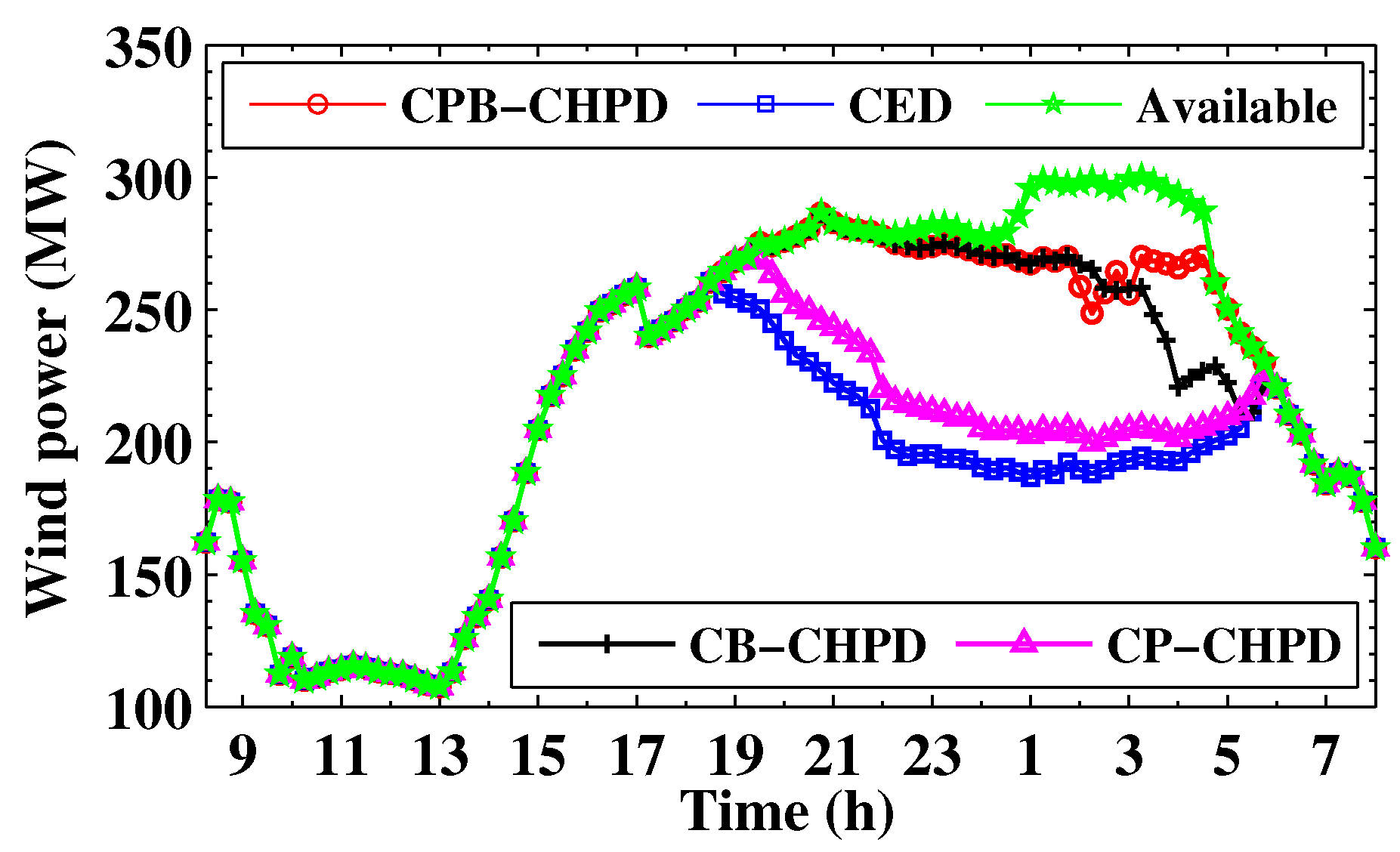
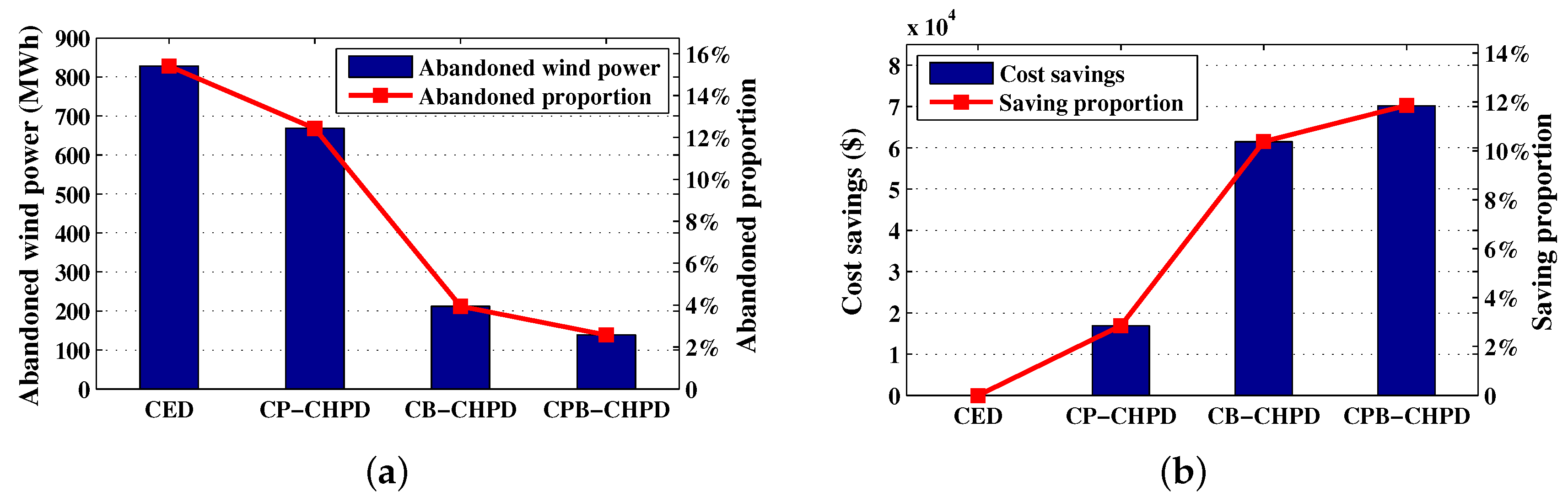
Figure 8 shows the electric power output of the wind farm of the four dispatch models at each period. The optimization results of wind power integration and operation cost savings are given in Table 4. Based on these data, the histograms of the amount of abandoned wind power and operation cost savings are shown in Figure 10.
It is observed that, the capability of wind power integration increases in the order of the CED, CP-CHPD, CB-CHPD and CPB-CHPD models as shown in Figure 10a, and so do the operation cost savings, as shown in Figure 10b. In Table 4, based on the CED model, the other three models utilize more wind power energy by 159.54 MWh, 616.22 MWh and 689.71 MWh respectively, and they save more operation cost by $16,866, $61,455 and $70,172 respectively.
The amount of wind power energy integration and operation cost savings of the CB-CHPD model are more than those of the CP-CHPD model, which indicates that the CB-CHPD model makes the power and heat decoupling better than the CP-CHPD model. That is because the heat storage capacity of pipelines is much smaller than that of the buildings group. Further, the CPB-CHPD model can significantly exploit the synergic effects of PDTP and BTI to realize the power and heat decoupling more fully.
This case indicates that each of the other three models (the CP-CHPD, CB-CHPD and CPB-CHPD models) has a good performance on wind power integration and operation economic benefits, while the CPB-CHPD model involving PDTP and BTI together has much better synergic benefits.
5. Conclusions
The coordination of pipelines and buildings heat storage can be utilized to break the strong linkage of electric power and heat supply of the CHP units more effectively, which can improve the system operational flexibility, with enhancing wind power integration and reducing total operation cost significantly. Several simulation tests demonstrate that the proposed CPB-CHPD model has a good performance on power and heat decoupling. The detailed results are summarized as follows.
Coordinating the generation of every electric power and heat supply source in the combined heat and power system can introduce significant system operational flexibility just by considering PDTP and BTI without any additional investment. This method need not adjust the configuration of electric power and heat supply sources or impact end users’ heat supply quality. The CPB-CHPD model can utilize more wind power energy than the CED model accounting for approximate , and the total operation cost is reduced by nearly .
The combined heat and power dispatch models considering PDTP or BTI can realize power and heat decoupling, where the effect of the latter BTI is more obvious than that of the former PDTP. However, the model considering both PDTP and BTI has much better synergic benefits. Based on the CED model, the CP-CHPD model can integrate more wind power energy and save more operation cost by approximate and , respectively, and the CB-CHPD model correspondingly and .
There is an interesting issue worth more study. In the large-scale electric power system, a simple equivalent model representing the heat storage capacity of pipelines and buildings in the district heating system may be concerned rather than the detailed and complex model to reduce the solving complexity of the combined heat and power dispatch model.
Acknowledgments
This work was supported by the National Natural Science Foundation of China (NSFC) (51607021).
Author Contributions
Ping Li and Weidong Li conceived of and designed the research problem. Ping Li wrote the whole manuscript. Weidong Li supervised the paper writing. Haixia Wang and Quan Lv participated in the results analysis.
Conflicts of Interest
The authors declare no conflict of interest.
Abbreviations
| CHP | Combined heat and power |
| CON | Condensing power |
| EPS | Electric power system |
| DHS | District heating system |
| PDTP | Pipelines dynamic thermal performance |
| BTI | Buildings thermal inertia |
| CPB-CHPD | Combined heat and power dispatch considering both PDTP and BTI |
| CP-CHPD | Combined heat and power dispatch only considering PDTP |
| CB-CHPD | Combined heat and power dispatch only considering BTI |
| CED | Conventional economic dispatch considering neither PDTP, nor BTI |
References
- Chinese Renewable Energy Industries Association (CREIA). China Wind Power Review and Outlook 2016; CREIA: Beijing, China, 2016. (In Chinese) [Google Scholar]
- Streckiené, G.; Martinaitis, V.; Andersen, A.N.; Katz, J. Feasibility of CHP-plants with thermal stores in the German spot market. Appl. Energy 2009, 86, 2308–2316. [Google Scholar] [CrossRef]
- Celador, A.C.; Odriozola, M.; Sala, J.M. Implications of the modelling of stratified hot water storage tanks in the simulation of CHP plants. Energy Convers. Manag. 2011, 52, 3018–3026. [Google Scholar] [CrossRef]
- Rong, S.; Li, Z.; Li, W. Investigation of the promotion of wind power consumption using the thermal-electric decoupling techniques. Energies 2015, 8, 8613–8629. [Google Scholar] [CrossRef]
- Yuan, R.; Ye, J.; Lei, J.; Li, T. Integrated combined heat and power system dispatch considering electrical and thermal energy storage. Energies 2016, 9, 474. [Google Scholar] [CrossRef]
- Chen, H.; Yu, Y.; Jiang, X. Optimal scheduling of combined heat and power units with heat storage for the improvement of wind power integration. In Proceedings of the 2016 IEEE PES Asia-Pacific Power and Energy Engineering Conference (APPEEC), Xi’an, China, 25–28 October 2016; pp. 1508–1512. [Google Scholar] [CrossRef]
- Mathiesen, B.V.; Lund, H. Comparative analyses of seven technologies to facilitate the integration of fluctuating renewable energy sources. IET Renew. Power Gener. 2009, 3, 190–204. [Google Scholar] [CrossRef]
- Long, H.; Xu, R.; He, J. Incorporating the variability of wind power with electric heat pumps. Energies 2011, 4, 1748–1762. [Google Scholar] [CrossRef]
- Papaefthymiou, G.; Hasche, B.; Nabe, C. Potential of heat pumps for demand side management and wind power integration in the German electricity market. IEEE Trans. Sustain. Energy 2012, 3, 636–642. [Google Scholar] [CrossRef]
- Chen, X.; Kang, C.; O’Malley, M.; Xia, Q.; Bai, J.; Liu, C.; Sun, R.; Wang, W.; Li, H. Increasing the flexibility of combined heat and power for wind power integration in China: Modeling and implications. IEEE Trans. Power Syst. 2015, 30, 1848–1857. [Google Scholar] [CrossRef]
- Zhang, N.; Lu, X.; McElroy, M.B.; Nielsen, C.P.; Chen, X.; Deng, Y.; Kang, C. Reducing curtailment of wind electricity in China by employing electric boilers for heat and pumped hydro for energy storage. Appl. Energy 2016, 184, 987–994. [Google Scholar] [CrossRef]
- Moradi, H.; Abtahi, A.; Esfahanian, M. Optimal energy management of a smart residential combined heat, cooling and power. Int. J. Tech. Phys. Probl. Eng. 2016, 8, 9–16. [Google Scholar]
- Moradi, H.; Moghaddam, I.G.; Moghaddam, M.P.; Haghifam, M.R. Opportunities to improve energy efficiency and reduce greenhouse gas emissions for a cogeneration plant. In Proceedings of the 2010 IEEE International Energy Conference and Exhibition (EnergyCon), Manama, Bahrain, 18–22 December 2010; pp. 785–790. [Google Scholar] [CrossRef]
- Ye, J.; Yuan, R. Integrated natural gas, heat, and power dispatch considering wind power and power-to-gas. Sustainability 2017, 9, 602. [Google Scholar] [CrossRef]
- Andersson, S. Influence of the net structure and operating strategy on the heat load of a district-heating network. Appl. Energy 1993, 46, 171–179. [Google Scholar] [CrossRef]
- Li, Z.; Wu, W.; Shahidehpour, M.; Wang, J.; Zhang, B. Combined heat and power dispatch considering pipeline energy storage of district heating network. IEEE Trans. Sustain. Energy 2016, 7, 12–22. [Google Scholar] [CrossRef]
- Jin, X.; Mu, Y.; Jia, H.; Wu, J.; Jiang, T.; Yu, X. Dynamic economic dispatch of a hybrid energy microgrid considering building based virtual energy storage system. Appl. Energy 2017, 194, 386–398. [Google Scholar] [CrossRef]
- Awad, B.; Chaudry, M.; Wu, J.; Jenkins, N. Integrated optimal power flow for electric power and heat in a microgrid. In Proceedings of the 20th International Conference and Exhibition on Electricity Distribution (CIRED), Prague, Czech Republic, 8–11 June 2009; pp. 869:1–869:4. [Google Scholar] [CrossRef]
- Jiang, X.; Jing, Z.; Li, Y.; Wu, Q.; Tang, W. Modelling and operation optimization of an integrated energy based direct district water-heating system. Energy 2014, 64, 375–388. [Google Scholar] [CrossRef]
- Li, J.; Fang, J.; Zeng, Q.; Chen, Z. Optimal operation of the integrated electrical and heating systems to accommodate the intermittent renewable sources. Appl. Energy 2016, 167, 244–254. [Google Scholar] [CrossRef]
- Zhao, H.; Bohm, B.; Ravn, H.F. On optimum operation of a CHP type district heating system by mathematical modeling. Euroheat Power 1995, 24, 618–622. [Google Scholar]
- Zhao, H. Analysis, Modelling and Operational Optimization of District Heating Systems. Ph.D. Thesis, Technical University of Denmark, Copenhagen, Denmark, 1995. [Google Scholar]
- Fu, L.; Jiang, Y. Optimal operation of a CHP plant for space heating as a peak load regulating plant. Energy 2000, 25, 283–298. [Google Scholar] [CrossRef]
- Wernstedt, F.; Davidsson, P.; Johansson, C. Demand side management in district heating systems. In Proceedings of the 6th International Joint Conference on Autonomous Agents and Multiagent Systems (AAMAS’07), Honolulu, HI, USA, 14–18 May 2007; pp. 1383–1389. [Google Scholar] [CrossRef]
- Kensby, J.; Trüschel, A.; Dalenbäck, J.O. Potential of residential buildings as thermal energy storage in district heating systems—Results from a pilot test. Appl. Energy 2015, 137, 773–781. [Google Scholar] [CrossRef]
- Brange, L.; Englund, J.; Lauenburg, P. Prosumers in district heating networks—A Swedish case study. Appl. Energy 2016, 164, 492–500. [Google Scholar] [CrossRef]
- Satyavada, H.; Baldi, S. An integrated control-oriented modelling for HVAC performance benchmarking. J. Build. Eng. 2016, 6, 262–273. [Google Scholar] [CrossRef]
- Satyavada, H.; Babus̆ka, R.; Baldi, S. Integrated dynamic modelling and multivariable control of HVAC components. In Proceedings of the 2016 European Control Conference (ECC), Aalborg, Denmark, 29 June–1 July 2016; pp. 1171–1176. [Google Scholar] [CrossRef]
- Yang, Y.; Wu, K.; Long, H.; Gao, J.; Yan, X.; Kato, T.; Suzuoki, Y. Integrated electricity and heating demand-side management for wind power integration in China. Energy 2014, 78, 235–246. [Google Scholar] [CrossRef]
- Wu, C.; Jiang, P.; Gu, W.; Sun, Y. Day-ahead optimal dispatch with CHP and wind turbines based on room temperature control. In Proceedings of the 2016 IEEE International Conference on Power System Technology (POWERCON), Wollongong, Australia, 28 September–1 October 2016; pp. 1–6. [Google Scholar] [CrossRef]
- Pan, Z.; Guo, Q.; Sun, H. Feasible region method based integrated heat and electricity dispatch considering building thermal inertia. Appl. Energy 2017, 192, 395–407. [Google Scholar] [CrossRef]
- Li, P.; Nord, N.; Ertesvåg, I.S.; Ge, Z.; Yang, Z.; Yang, Y. Integrated multiscale simulation of CHP based district heating system. Energy Convers. Manag. 2015, 106, 337–354. [Google Scholar] [CrossRef]
- Pan, Z.; Guo, Q.; Sun, H. Interactions of district electricity and heating systems considering time-scale characteristics based on quasi-steady multi-energy flow. Appl. Energy 2016, 167, 230–243. [Google Scholar] [CrossRef]
- Andersen, T.V. Integration of 50% Wind Power in a CHP-Based Power System: A Model-Based Analysis of the Impacts of Increasing Wind Power and the Potentials of Flexible Power Generation. Ph.D. Thesis, Technical University of Denmark, Copenhagen, Denmark, 2009. [Google Scholar]
- Liu, X.; Wu, J.; Jenkins, N.; Bagdanavicius, A. Combined analysis of electricity and heat networks. Appl. Energy 2015, 162, 1238–1250. [Google Scholar] [CrossRef]
- Sandou, G.; Font, S.; Tebbani, S.; Hiret, A.; Mondon, C. Predictive control of a complex district heating network. In Proceedings of the 44th IEEE Conference on Decision and Control, 2005 and 2005 European Control Conference (CDC-ECC’05), Seville, Spain, 12–15 December 2005; pp. 7372–7377. [Google Scholar] [CrossRef]
- Arvastson, L. Stochastic Modelling and Operational Optimization in District Heating Systems. Ph.D. Thesis, Lund Institute of Technology, Lund, Sweden, 2001. [Google Scholar]
- Lu, N. An evaluation of the HVAC load potential for providing load balancing service. IEEE Trans. Smart Grid 2012, 3, 1263–1270. [Google Scholar] [CrossRef]
Figure 1.
Electric and heat power characteristics of the CHP units.
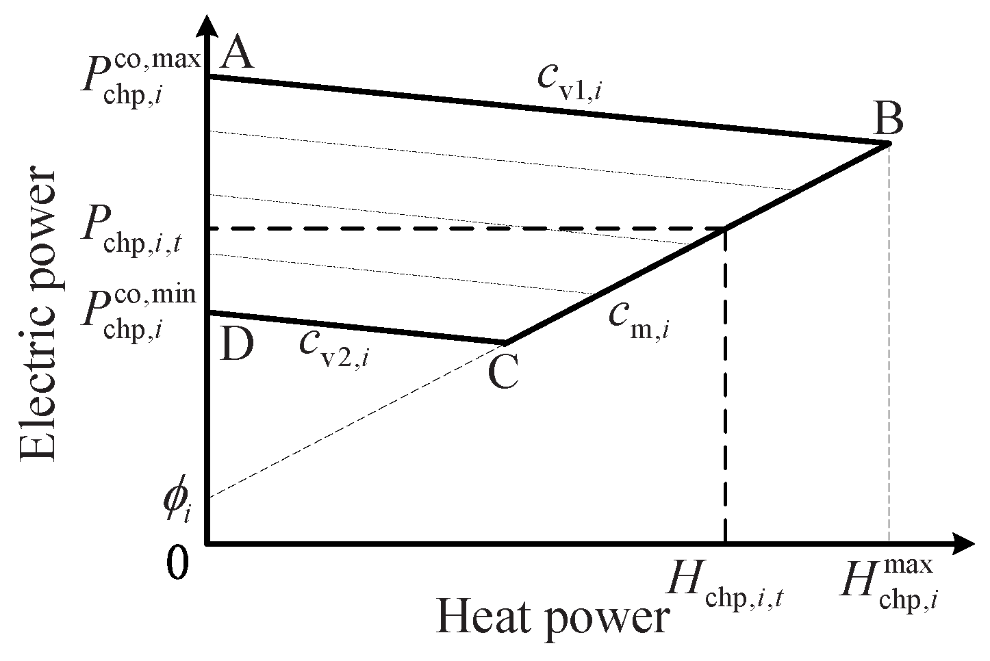
Figure 2.
General structure of a single pipeline.

Figure 3.
General structure of a node connecting with cross pipelines.

Figure 4.
Configuration of the combined heat and power simulation system.

Figure 5.
Profiles of the typical day during the heating season: (a) total electric loads and forecast wind power; (b) outdoor temperature.
Figure 5.
Profiles of the typical day during the heating season: (a) total electric loads and forecast wind power; (b) outdoor temperature.

Figure 6.
Electric power output of the thermal power units at each period in Case 1: (a) the first CHP unit CHP1; (b) the second CHP unit CHP2; (c) the first CON unit CON1; (d) the second CON unit CON2.
Figure 6.
Electric power output of the thermal power units at each period in Case 1: (a) the first CHP unit CHP1; (b) the second CHP unit CHP2; (c) the first CON unit CON1; (d) the second CON unit CON2.

Figure 7.
Heat power output of the CHP units at each period in Case 1: (a) the first CHP unit CHP1; (b) the second CHP unit CHP2.
Figure 7.
Heat power output of the CHP units at each period in Case 1: (a) the first CHP unit CHP1; (b) the second CHP unit CHP2.
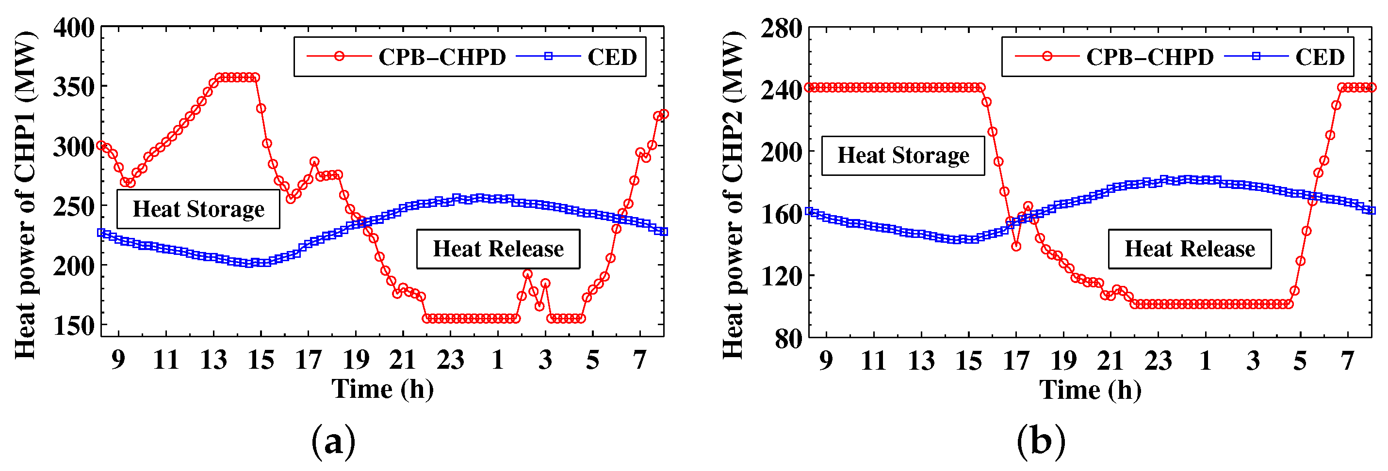
Figure 8.
Electric power output of the wind farm of the four dispatch models at each period, including the CPB-CHPD, CB-CHPD, CP-CHPD models (combined heat and power dispatch models considering both PDTP and BTI, only BTI, only PDTP, respectively) and the CED model (conventional economic dispatch model considering neither PDTP, nor BTI).

Figure 9.
Profiles of indoor temperatures in Case 1 at each period: (a) Building1; (b) Building2; (c) Building3; (d) Building4; (e) Building5 ; (f) Building6.
Figure 9.
Profiles of indoor temperatures in Case 1 at each period: (a) Building1; (b) Building2; (c) Building3; (d) Building4; (e) Building5 ; (f) Building6.
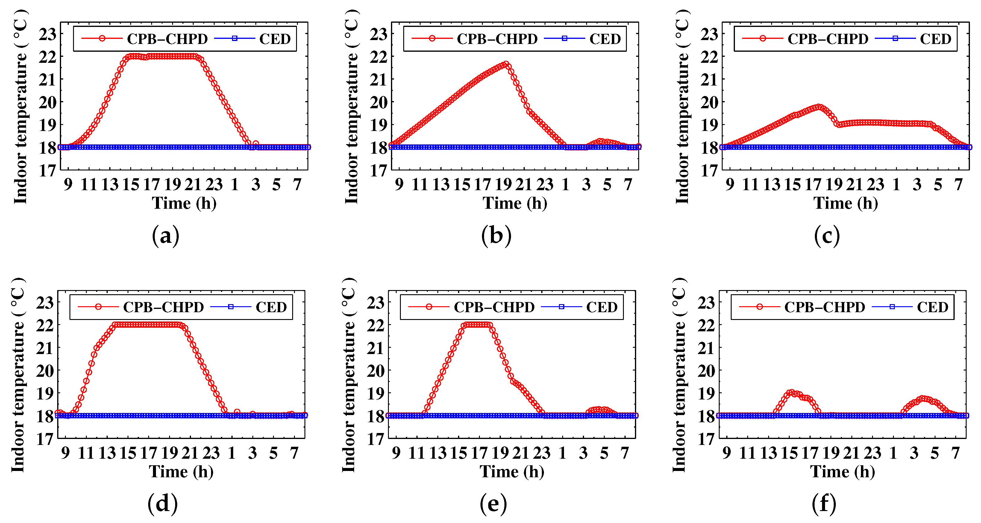
Figure 10.
Optimal result comparison of the four dispatch models, including the CPB-CHPD, CB-CHPD, CP-CHPD and CED models: (a) abandoned wind power; (b) operation cost savings.
Figure 10.
Optimal result comparison of the four dispatch models, including the CPB-CHPD, CB-CHPD, CP-CHPD and CED models: (a) abandoned wind power; (b) operation cost savings.


Table 1.
Parameters of thermal power units.
| Type | CHP Units | CON Units | ||
|---|---|---|---|---|
| Unit name | CHP1 | CHP2 | CON1 | CON2 |
| Capacity () | 300 | 200 | 500 | 200 |
| () | 323 | 212 | / | / |
| () | 150 | 100 | 200 | 80 |
| () | 357 | 241 | / | / |
| 0.23 | 0.21 | / | / | |
| 0 | 0 | / | / | |
| 0.45 | 0.44 | / | / | |
| Ramping rate () | 80 | 50 | 100 | 50 |
Table 2.
Parameters of pipelines.
| No. | () | () | () |
|---|---|---|---|
| 1, 2, 11, 12 | 3250 | 0.8 | 32 |
| 3, 4, 5, 6, 13, 14, 15, 16 | 1500 | 0.6 | 32 |
| 7, 8, 9, 10, 17, 18, 19, 20 | 1050 | 0.5 | 32 |
Table 3.
Parameters of buildings.
| No. | () | () | Equivalent area () |
|---|---|---|---|
| 1 | 1.85 | 16.20 | 1.32 |
| 2 | 2.45 | 12.60 | 1.74 |
| 3 | 2.95 | 10.08 | 2.09 |
| 4 | 1.45 | 13.68 | 1.16 |
| 5 | 1.75 | 10.44 | 1.40 |
| 6 | 1.95 | 8.64 | 1.56 |
Table 4.
Wind power integration and operation cost savings of the four dispatch models including the CPB-CHPD, CB-CHPD, CP-CHPD and CED models.
Table 4.
Wind power integration and operation cost savings of the four dispatch models including the CPB-CHPD, CB-CHPD, CP-CHPD and CED models.
| Wind Power Integration () | Total Operation Costs ($) | Cost Savings Based on CED ($) | Saving Proportion Based on CED | |
|---|---|---|---|---|
| CPB-CHPD | 5239.68 | 521,741 | 70,172.55 | 11.86% |
| CB-CHPD | 5166.19 | 530,458 | 61,455.19 | 10.38% |
| CP-CHPD | 4709.51 | 575,062 | 16,866.53 | 2.85% |
| CED | 4549.97 | 591,929 | / | / |
© 2017 by the authors. Licensee MDPI, Basel, Switzerland. This article is an open access article distributed under the terms and conditions of the Creative Commons Attribution (CC BY) license (http://creativecommons.org/licenses/by/4.0/).
Share and Cite
MDPI and ACS Style
Li, P.; Wang, H.; Lv, Q.; Li, W. Combined Heat and Power Dispatch Considering Heat Storage of Both Buildings and Pipelines in District Heating System for Wind Power Integration. Energies 2017, 10, 893. https://doi.org/10.3390/en10070893
AMA Style
Li P, Wang H, Lv Q, Li W. Combined Heat and Power Dispatch Considering Heat Storage of Both Buildings and Pipelines in District Heating System for Wind Power Integration. Energies. 2017; 10(7):893. https://doi.org/10.3390/en10070893
Chicago/Turabian StyleLi, Ping, Haixia Wang, Quan Lv, and Weidong Li. 2017. "Combined Heat and Power Dispatch Considering Heat Storage of Both Buildings and Pipelines in District Heating System for Wind Power Integration" Energies 10, no. 7: 893. https://doi.org/10.3390/en10070893
Note that from the first issue of 2016, this journal uses article numbers instead of page numbers. See further details here.