
A New Miniature Wind Turbine for Wind Tunnel Experiments. Part II: Wake Structure and Flow Dynamics


Wind Engineering and Renewable Energy Laboratory (WIRE), École Polytechnique Fédérale de Lausanne (EPFL), EPFL-ENAC-IIE-WIRE, 1015 Lausanne, Switzerland
*
Author to whom correspondence should be addressed.
Energies 2017, 10(7), 923; https://doi.org/10.3390/en10070923
Submission received: 10 May 2017
/
Revised: 24 June 2017
/
Accepted: 29 June 2017
/
Published: 4 July 2017
(This article belongs to the Collection Wind Turbines)
Abstract
:An optimized three-bladed horizontal-axis miniature wind turbine, called WiRE-01, with the rotor diameter of 15 cm is designed and fully characterized in Part I of this study. In the current part of the study, we investigate the interaction of the turbine with a turbulent boundary layer. The comparison of the spectral density of the thrust force and the one of the incoming velocity revealed new insights on the use of turbine characteristics to estimate incoming flow conditions. High-resolution stereoscopic particle image-velocimetry (S-PIV) measurements were also performed in the wake of the turbine operating at optimal conditions. Detailed information on the velocity and turbulence structure of the turbine wake is presented and discussed, which can serve as a complete dataset for the validation of numerical models. The PIV data are also used to better understand the underlying mechanisms leading to unsteady loads on a downstream turbine at different streamwise and spanwise positions. To achieve this goal, a new method is developed to quantify and compare the effect of both turbulence and mean shear on the moment of the incoming momentum flux for a hypothetical turbine placed downstream. The results show that moment fluctuations caused by turbulence are bigger under full-wake conditions, whereas those caused by mean shear are clearly dominant under partial-wake conditions. Especial emphasis is also placed on how the mean wake flow distribution is affected by wake meandering. Conditional averaging based on the instantaneous position of the wake center revealed that when the wake meanders laterally to one side, a high-speed region exists on the opposite side. The results show that, due to this high-speed region, large lateral meandering motions do not lead to the expansion of the mean wake cross-section in the lateral direction.
1. Introduction
Based on the energy outlook report published by the U.S. Energy Information Administration (EIA) [1] in 2016, renewables are the fastest growing energy source in the world with a projected increase of 2.6% per year from 2012 to 2040. A significant part of this fast growth is expected to come from the continuing boost in global wind power production. To maximize wind power production and minimize maintenance cost, a very common practice is to install multiple wind turbines close to each other as a group, thus forming a wind farm. The major existing challenge in wind farms is, however, wind turbine wakes. Turbine wakes are characterized by a decrease in velocity and an increase in turbulence. The former leads to the power reduction of downstream turbines while the latter increases harmful unsteady structural loads on downstream turbines.
Extensive research has been performed in the literature to understand and predict turbine wake characteristics using different numerical and experimental methods (see the reviews of [2,3,4,5,6]). Early works (e.g., [7]) studied turbine wakes under uniform inflow conditions. However, the interaction of turbine wakes with boundary-layer flows has gradually received more attention in the wind energy community as wind turbines operate in the atmospheric boundary-layer (ABL) flow. In particular, during the last ten years, wind tunnel experiments (e.g., [8,9,10,11,12,13,14,15,16,17,18,19]) have been performed to study wakes of down-scaled wind turbines in boundary-layer flows. These works sought to provide a better understanding on turbine wake characteristics. However, some essential wake characteristics are still far from being well understood. For instance, despite the recent attention given to wake meandering in the literature (e.g., [20,21,22,23]), the effect of meandering motions on flow distribution in turbine wakes is not well understood yet. As another example, the power reduction of downstream turbines caused by wake flows has been extensively studied (e.g., [24,25,26,27,28]) but relatively less attention has been given to unsteady structural loads induced by wake flows on downstream turbines. In general, both turbulence and mean shear in turbine wakes induce unsteady structural loads on rotating blades of downstream turbines. It is of great interest therefore to try to quantify and compare the effects of turbulence and mean shear on unsteady structural loads for downstream turbines under different wind-farm layout configurations.
The data obtained from wind tunnel experiments of turbine wakes under boundary-layer inflow conditions (e.g., [8]) have been also commonly used as a benchmark to validate numerical models (e.g., [29,30]). However, miniature turbines employed in these studies usually have poor performance with respect to large-scale turbines in the field, or their performance is not fully and properly characterized. As turbine characteristics can significantly affect wake flows [31], it is important that miniature turbines have more realistic characteristics (similar to those of utility-scale turbines). Moreover, turbine characteristics (e.g., thrust and power coefficients, tip-speed ratio and twist/chord distributions) should be fully provided for those who aim at using the wind tunnel data to validate their numerical models.
In Part I of this study [32], a new optimized miniature turbine with realistic characteristics is designed and fully characterized. In the current part of the study, the interaction of the new turbine with a boundary-layer flow is studied. The remainder of the paper is organized as follows. In Section 2, experimental setup is presented. Section 3 concerns the connection between the dynamic behaviour of the incoming flow and the one of the turbine thrust force. The data obtained from stereo particle image-velocimetry (S-PIV) measurements are employed in Section 4 to present and discuss the velocity and turbulence structure in the turbine wake. A new method is developed in Section 5 to assess and compare incoming flow unsteadiness due to both turbulence and mean shear for a hypothetical turbine placed in the turbine wake at different streamwise and spanwise positions. In Section 6, conditional averaging is performed on the wake velocity data to study wake meandering and its effect on mean flow distribution. Finally, a summary is presented in Section 7.
2. Experimental Setup
The new miniature wind turbine (WiRE-01) with the diameter of 15 cm was placed in the atmospheric boundary-layer wind tunnel of WiRE laboratory at EPFL, Switzerland. The test section of the wind tunnel is 28 m long, 2.6 m wide and 2 m high. Due to the very small frontal area of the turbine with respect to the wind tunnel cross-section, blockage effects are found to be negligible. Detailed information about the new rotor can be found in Part I of this study [32]. The turbine hub height is selected to be 12.5 cm in order to have a ratio of similar to the one of large-scale turbines in the field. The turbine nacelle has a diameter and length of 10 mm and 35 mm, respectively, and the tower has a diameter and length of 4.6 mm and 125 mm, respectively. A schematic figure of the miniature wind turbine is shown in Figure 1a. Due to the long test section of the wind tunnel, the boundary layer is naturally developed over the floor without the need of any tripping mechanism. A single hot-wire anemometer was used to characterize the incoming boundary-layer profile. Velocity measurements were performed in a vertical profile from cm up to 48 cm. At each position, the data were sampled at a rate of 15 kHz for a period of 120 s. Figure 2a,b shows the profiles of the normalized mean incoming velocity and the turbulence intensity , respectively, where is the incoming streamwise velocity at the turbine hub height and denotes the value of the standard deviation. The overbar denotes time averaging. The value of the mean incoming velocity and turbulence intensity at hub height are kept constant at 5 and , respectively. The boundary-layer thickness is approximately 40 cm at the measurement location. This gives that is similar to the case of off-shore wind turbines [33]. The friction velocity and the aerodynamic surface roughness length are estimated to be 0.21 and mm, respectively, based on fitting a logarithmic curve to the measured points in the surface layer (lowest of the boundary layer). The boundary-layer profile can be also approximated with a power-law relationship given by , where is the mean free-stream velocity. The value of the power-law exponent n for the fitted curve shown by the solid line in Figure 2a is . The variations of the thrust coefficient and the power coefficient versus the tip-speed ratio for the miniature turbine in the boundary layer is shown in Figure 1b. The values of thrust and power coefficients are given by
where T and P are the thrust force and the mechanical power of the turbine, respectively. d is the rotor diameter and is the air density. As shown in the figure and also discussed in Part I of this study [32], the new miniature turbine has more realistic values of and compared to those usually employed in prior wind tunnel experiments (e.g., [8,13]) to study the interaction of wind turbines with turbulent boundary layers. The optimal tip-speed ratio at which the extracted power is maximum is also shown in Figure 1b. Note that, as seen in the figure, the miniature turbine has a small value of with respect to utility-scale turbines. The reader is referred to Section 2.3 of Part I of this study [32] for the detailed discussion on the origin of this difference. It is also worth mentioning that the direct-current (DC) generator connected to the rotor in these measurements is relatively small (with a diameter of 1 cm) in order to minimize nacelle interferences on the wake flow. Power measurements were not therefore performed at tip-speed ratios lower than 2.5 as the shaft torque at this tip-speed ratio is beyond the operating range of the DC machine. See Part I of the study [32] for detailed discussion on the variation of and with the tip-speed ratio .
In addition, a high-resolution S-PIV system from LaVision was employed to measure the three velocity components in planes normal to the incoming flow (i.e., planes, where y and z denote the lateral and vertical directions, respectively). A 400 mJ dual-head Nd:Yag laser together with two 16-bit sCMOS cameras (2560 × 2160 pixels) was used to capture the wake flow in field of views (FOVs) with the size of and the spatial resolution of . The mean velocity field was obtained by ensemble averaging 1200 instantaneous velocity fields, and the data were sampled with a frequency of 10 Hz. Velocity measurements were performed for the incoming flow as well as the wake of the turbine operating at the optimal tip-speed ratio (). Figure 2c shows the profile of the vertical turbulent momentum flux normalized with for the incoming boundary layer flow. PIV data of the turbine wake will be discussed in detail in Section 4.
3. Dynamic Characteristics of Incoming Velocity Versus Thrust Force
Recent works (e.g., [34,35]) have shown the potential of using the information related to the wind-turbine performance to provide insights on the incoming-flow characteristics. In order to extend this stream of research, we compare the spectral density of the thrust force T with the one of the incoming flow at hub height, as seen in Figure 3 for two different tip-speed ratios. For the sake of comparison, the spectral density of , whose mean value is equal to , is also plotted in the figure, where A is the rotor area. For each operating condition, thrust measurements were performed over a period of 60 s with a sampling frequency of 15 kHz. As shown in the figure, the thrust spectral density closely matches the one of at very low frequencies. As low-frequency scales contain most of the turbulent kinetic energy of a turbulent flow, this matching can be employed as a useful technique to estimate incoming flow characteristics. It will be of interest to examine this possibility for wind turbines operating in the field, where thrust measurements are more feasible and affordable than time-resolved velocity measurements.
With the increase of frequency, the spectral densities of T and start to deviate from each other. In particular, there are some very strong peaks in the spectral density of the thrust force occurring exactly at the rotational frequency of the rotor and its harmonics (shown by dashed black lines in Figure 3a,b) which is in agreement with what was reported by Hu et al. [13]. For the higher tip-speed ratio, there are also some peaks exactly at half of the rotational frequency and its harmonics (shown by dotted black lines in Figure 3b). We also observed similar peaks in the spectral density of the rotor thrust force: (i) when the rotor is placed in free-stream flows; and even (ii) when there is no incoming wind, and the rotor is rotated with a DC motor. Therefore, although it is tempting to relate these peaks to the flow interaction with the wind turbine, we believe that structural machinery defects are likely responsible for the observed peaks in the spectral density of the thrust force. The ones associated with and its harmonics can be caused by the vibrations due to the rotor mass imbalance, bent shaft and angular or parallel misalignments [36]. The ones with and its harmonics can be also related to the blade pass frequency (BPF) [37]. Finally, the peaks at and its harmonics that are seen for the higher tip-speed ratio can be mainly due to the mechanical looseness. For instance, it occurs if the shaft is not properly fitted into the rotor or the turbine baseplate is not entirely fixed to the ground. See Scheffer and Girdhar [36] for more information on the vibration analysis of rotating machines.
4. Wake Structure
Figure 4 shows contours of the normalized velocity deficit overlaid with vectors of in-plane velocity components in planes at different downstream locations, where and is the mean incoming velocity. As seen in the figure, the wake cross-section of the new miniature turbine is qualitatively similar to those reported in previous wind tunnel studies (e.g., [8,11,38]). However, the wake is significantly stronger for the new turbine in terms of both velocity deficit (due to high ) and rotation (due to high ) than the ones reported in the mentioned studies, under relatively similar incoming flow conditions. Vertical and lateral profiles of the normalized velocity deficit at hub level are shown in Figure 5 with solid lines. For the sake of comparison, vertical profiles of reported by Chamorro and Porté-Agel [10] are also shown with dashed lines. As seen in the figure, the wake velocity deficit for the new turbine is almost twice the one reported by Chamorro and Porté-Agel [10]. In addition, Figure 6 shows vertical profiles of the normalized spanwise velocity and lateral profiles of the normalized vertical velocity at hub level at different downstream locations. The data reported in Zhang et al. [11] are also shown in the figure with dashed lines. The figure shows that the vertical and lateral velocities are significantly bigger for the wake of the new turbine with respect to those reported by Zhang et al. [11]. Based on the conservation of angular momentum, a higher value of the shaft torque for the new turbine leads to the stronger wake rotation, as seen in Figure 6. Note that the wake rotation is not negligible for the new rotor even 6 rotor diameters downwind of the turbine.
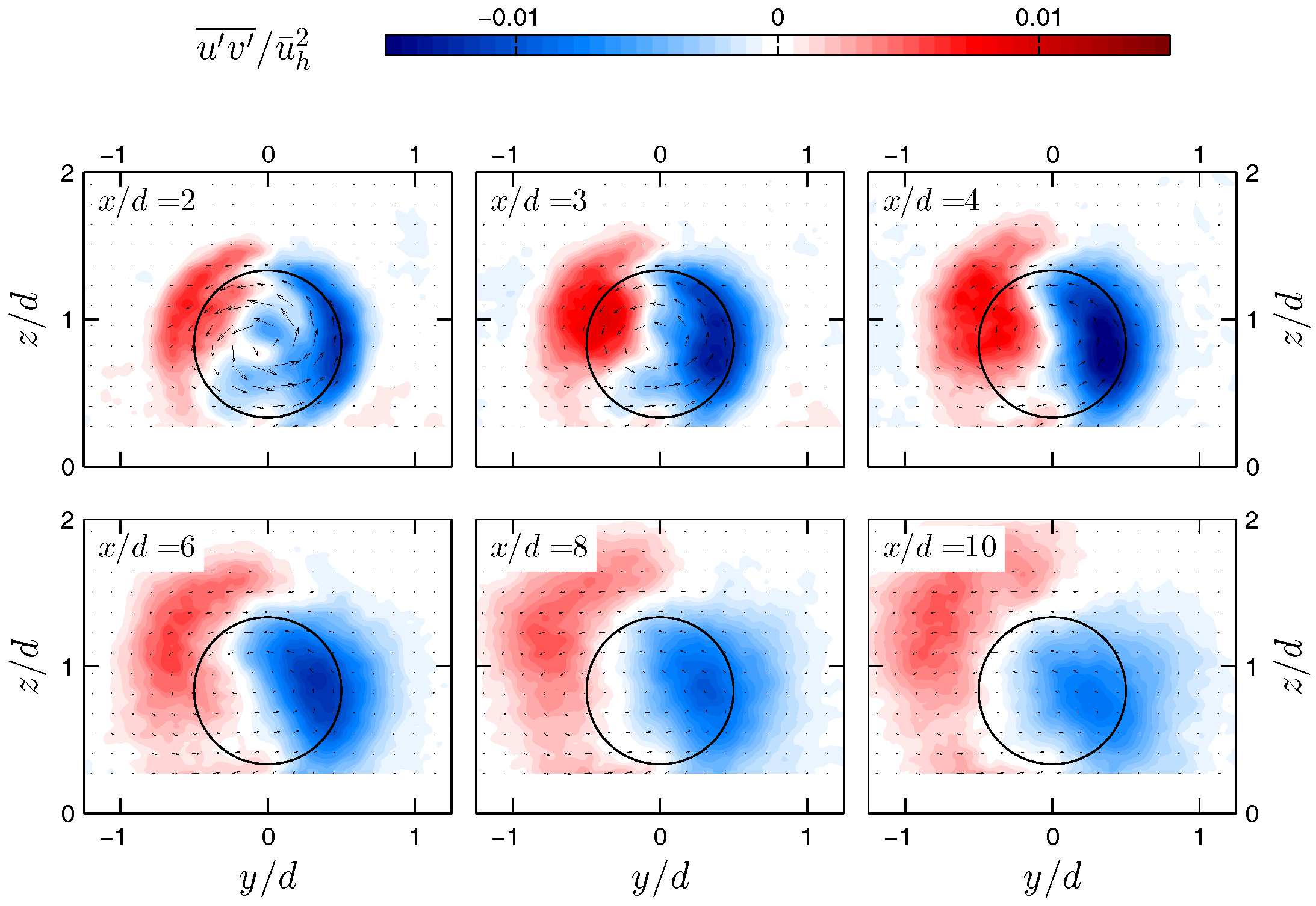
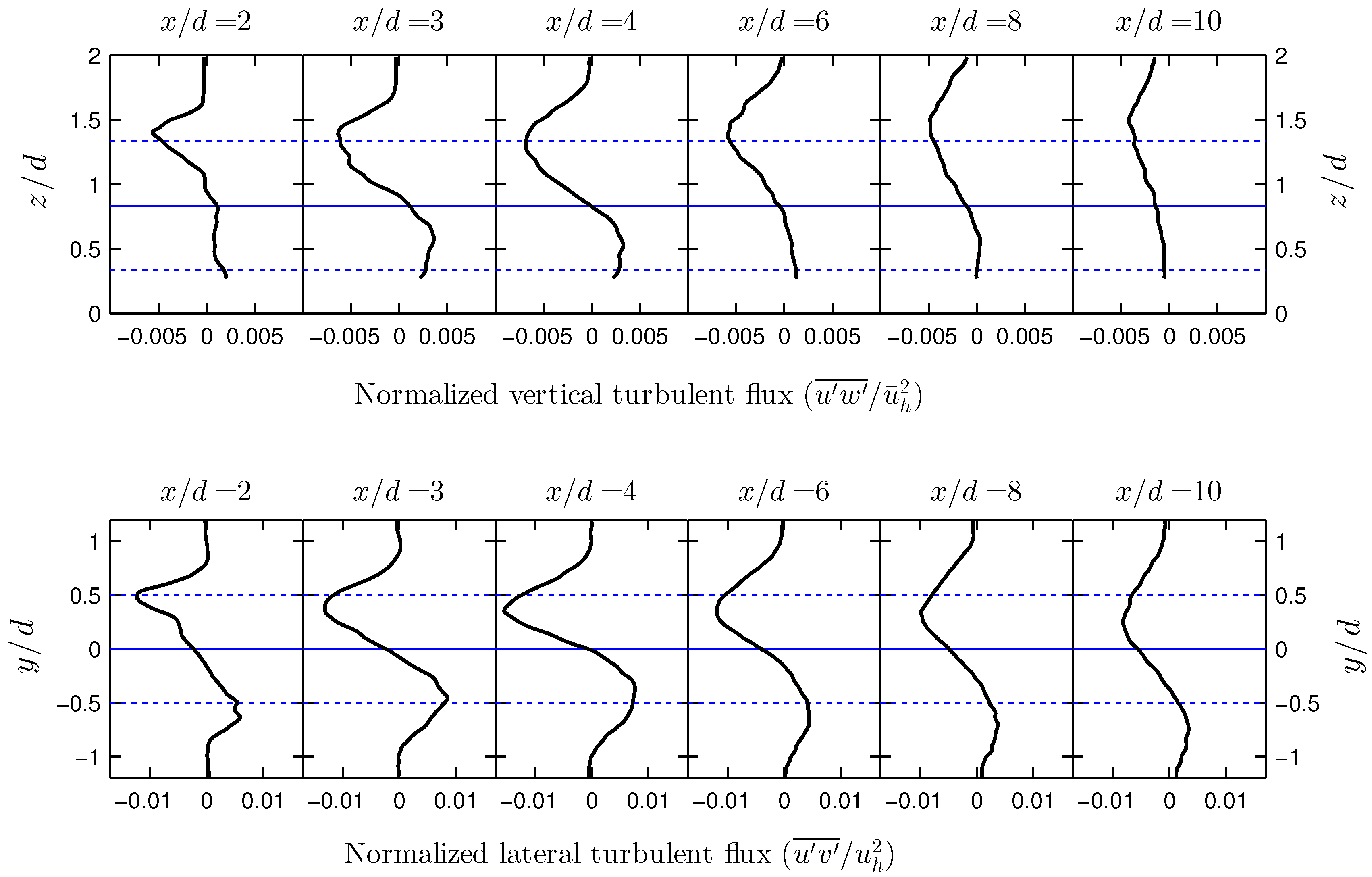
The wake recovery is usually associated with the turbulent momentum flux acting as a mechanism to transfer the energy from the outer flow into the wake. Figure 7 and Figure 8 show contours of the normalized vertical and lateral momentum fluxes (i.e., and ), respectively, at different downstream locations. To provide a more quantitative insight on the results, vertical profiles of the normalized vertical turbulent momentum flux as well as lateral profiles of the normalized lateral turbulent momentum flux at hub level are shown in Figure 9. As shown in Figure 7, Figure 8 and Figure 9, the maximum value of momentum turbulent fluxes occurs at around = 3–4, and they both have a non-symmetrical structure which is in agreement with previous studies (e.g., [8]). It is generally believed that the breakdown of tip vortices, which act as a a separating layer between the turbine wake and the outer flow [39], usually occurs at = 3–4. This results in a sudden increase of the flow entrainment at this region [8] . The tilting of turbulent flux distributions is also likely associated with the rotation of the wake [29]. Note also that the negative value of outside the turbine wake shown in Figure 7 is due to the fact that has a negative value in turbulent boundary layer flows over flat surfaces [40], as shown in Figure 2c for the incoming flow. Comparison of the profile of at seen in Figure 9 with the one of the incoming flow (Figure 2c) shows that the effect of the turbine can be still clearly seen at .
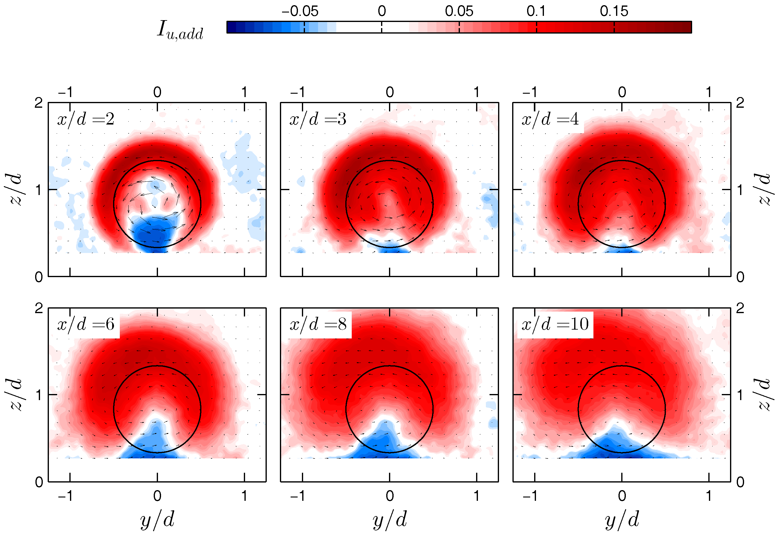
Figure 9 also shows that, for a given x, the maximum value of is higher than the one of , which has been reported by numerical studies of wake flows (e.g., [41]) as well. Even though more research has to be done to explain the reason for this, one possible explanation is that wake meandering motions are bigger in the lateral direction, discussed in detail in Section 6, which in turn enhance the flow entrainment in this direction. The streamwise turbulence intensity is one of the other important turbulence statistics of turbine wakes. The characterization of the turbulence intensity is of great importance as it induces harmful fatigue loads on blades of downstream turbines [42]. The turbulence intensity in turbine wakes consists of the turbulence intensity of the inflow and the one added (or subtracted) due to the presence of the turbine denoted by . The value of is given by [43]
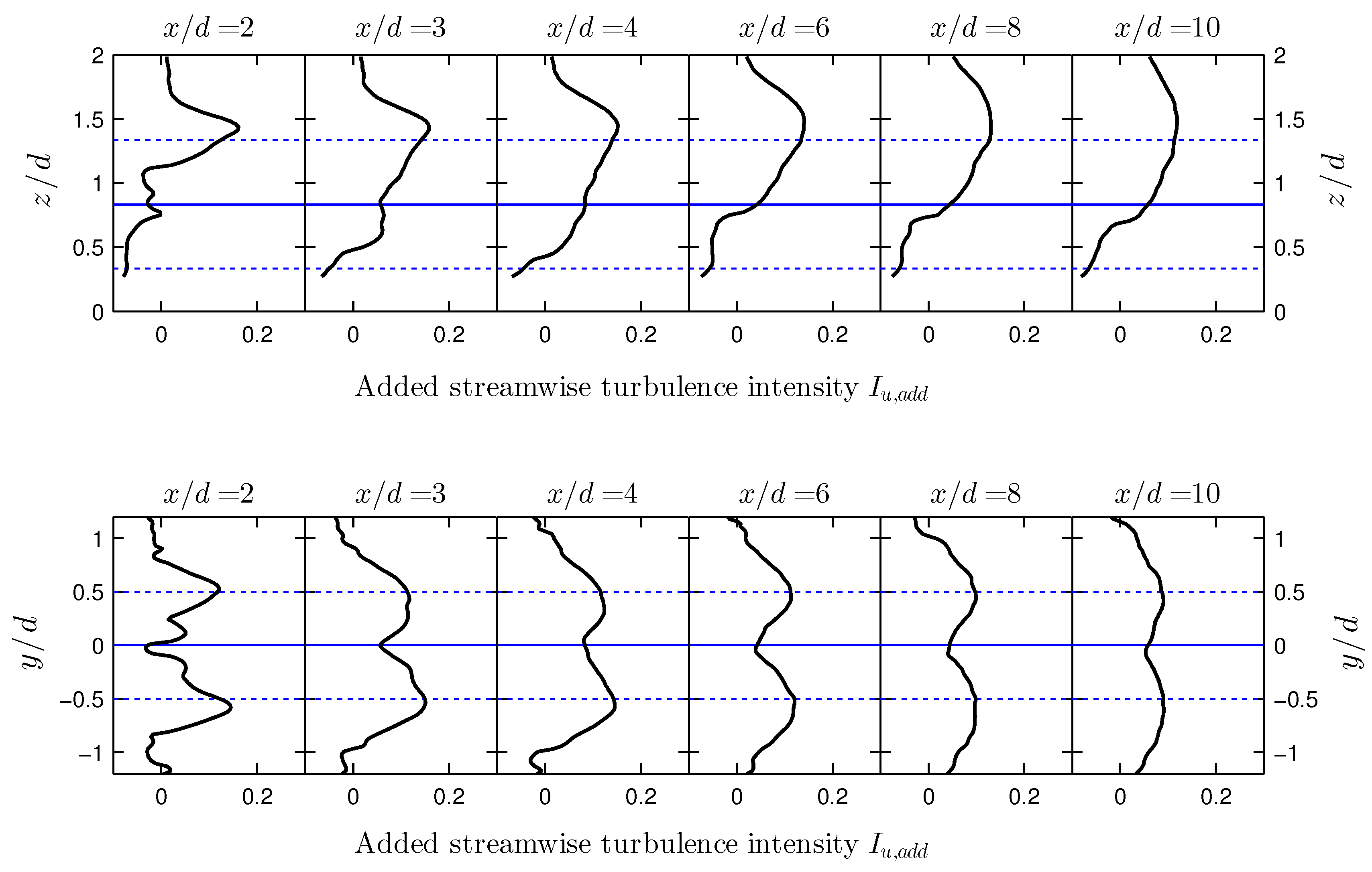
Figure 10 shows the contours of in planes at different downstream locations. As seen in the figure, the added streamwise turbulence intensity has a horseshoe shape with the maximum level close to the top-tip level. Moreover, the value of is negative downwind of the turbine bottom tip meaning that the turbine suppresses the turbulence in this region. This can be explained by the reduction of the mean flow shear near the ground [8], and consequently the reduction of the turbulence production in this region. To provide quantitative information on the turbine-induced turbulence, vertical and lateral profiles of at hub level are shown in Figure 11. The high level of added turbulence downwind of the top and the side tips of the rotor is clear in this figure.
5. Wake Flow Assessment: Fatigue Loads on Downstream Turbines
As mentioned earlier, it is quite common for wind turbines to work in the wake of upwind turbines in wind farms. In addition to the reduction in power production, this situation increases fatigue loads on wind turbines. In this section, we use the PIV data to investigate the unsteadiness of the wake flow at different positions. This helps us to have a better idea on the amount of unsteady loads on a wind turbine located downstream at different streamwise and spanwise positions.
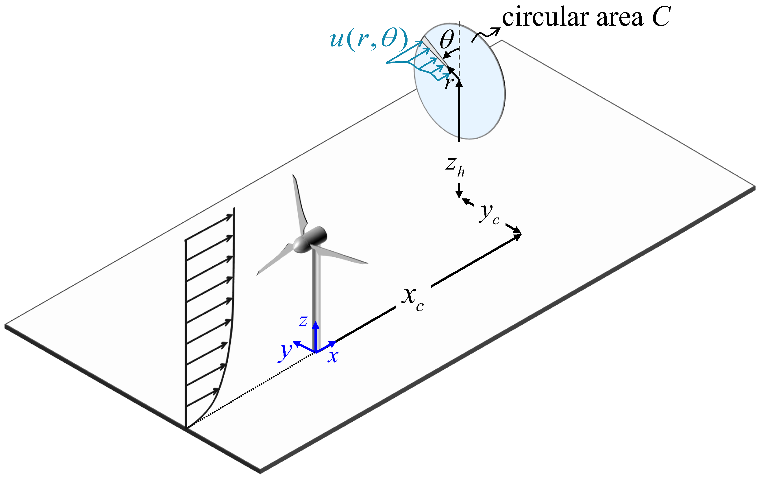
Let us consider the circular area C in a plane normal to the incoming flow (i.e., plane) with a diameter equal to the rotor diameter d, as shown in Figure 12. The center of C is located at , where and are arbitrary streamwise and spanwise positions, respectively, in the wake of the turbine. If a hypothetical turbine rotor is placed at C, the load moment on its blade root is given by
where is the acting force on the blade element at the radial position . As we know, the force acting on a blade element is proportional to the incoming momentum flux. Therefore, the equivalent moment (per unit area) of the incoming momentum flux for an infinitesimal circular sector element, shown in Figure 12, at the azimuthal angle of is equal to
where is the area of the infinitesimal circular sector element and . For any position of the circular area C in the turbine wake, the instantaneous value of at each azimuthal angle can be calculated based on the PIV data. The time-averaged moment (per unit area) for each azimuthal angle is thus equal to
The above equation states that is proportional to the sum of and although the former is usually significantly bigger than the latter. The time fluctuating part is also given by
Based on Equation 7, one can argue that time fluctuations of the moment is zero for laminar flows where , and it increases with the increase of both and in turbulent flows.
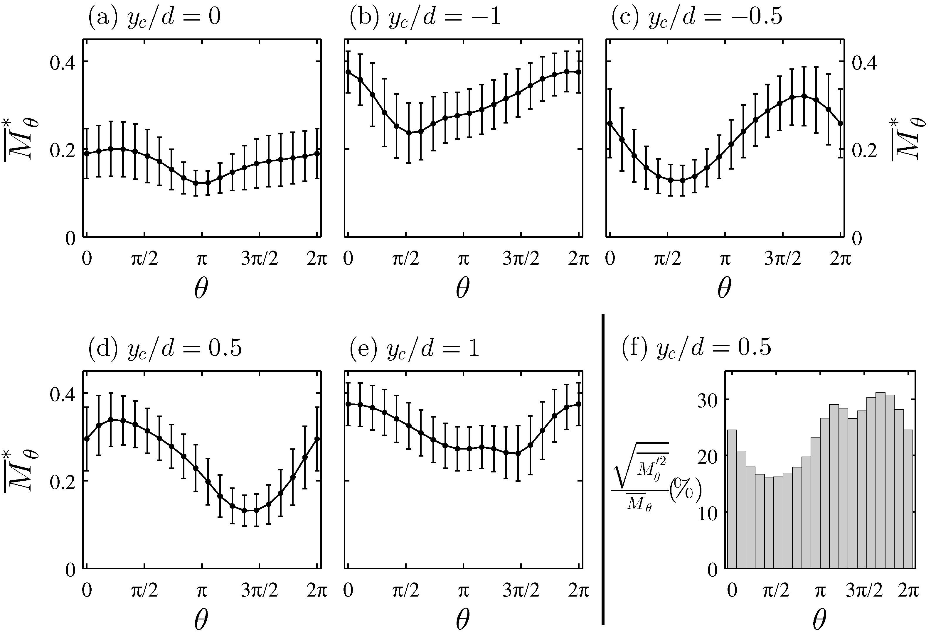
Figure 13a–e shows the variation of , non-dimensionalized with , with the azimuthal angle . The azimuthal angle is zero along the positive z-axis, and it increases towards the positive y-axis. As shown, each figure corresponds to a given while the value of is the same for all the figures, and it is equal to , which is in the typical range of turbine spacings in wind farms. Error bars in Figure 13a–e also indicate the value of the standard deviation of the moment , non-dimensionalized with .
Figure 13a corresponds to the case that the circular area C is in full-wake conditions (i.e., =0). The figure shows that is minimum at which can be explained by the lower value of at this azimuthal angle due to the boundary-layer shear flow. In addition to the low value of , velocity fluctuations are reduced at this azimuthal angle in the turbine wake as shown in Figure 10. Moment fluctuations have to be therefore minimum at this azimuthal angle, as shown in Figure 13a.
In Figure 13b,c, is not equal to zero, meaning that the circular area C is in partial-wake conditions. In general, the figures show that is minimum at where the velocity is smaller due to the turbine wake. At this azimuthal angle, it can be also seen that the value of is maximum for while it is minimum for (see the error bars in Figure 13b,c). In order to explain this difference, one has to recall that, based on Equation 7, moment fluctuations depend on both and . For , the circular area C only interacts with the border of the turbine wake, where velocity fluctuations are very large (see Figure 10) but is not drastically reduced by the turbine wake. As a result, moment fluctuations increase at this azimuthal angle. For , however, the value of is quite small at , which results in a reduction in moment fluctuations in this case despite the increase of . Similar discussions can be made for moment variations with at and shown in Figure 13d,e. For these cases, however, is the azimuthal angle at which C has the maximum overlap with the turbine wake. It is also of interest to examine the variation of with . This is shown in Figure 13f for and . As seen in the figure, the ratio of the standard deviation to the mean value is maximum at around even though the moment standard deviation is minimum at this azimuthal angle (Figure 13d).
As discussed earlier, flow turbulent fluctuations lead to moment fluctuations (shown by error bars in Figure 13a–e at each azimuthal angle. Apart from these fluctuations, we see in Figure 13a–e that varies with , caused by mean flow shear due to: (i) the incoming boundary layer; and (ii) the velocity reduction in the turbine wake. The variation of with leads to unsteady loads on the root of the rotating blade of the hypothetical turbine located at C. In order to quantify moment oscillations due to mean flow shear, one can calculate the value of at each azimuthal angle, where , and denotes spatial averaging over the azimuthal angles from 0 to . In other words, at each time instant and each azimuthal angle.
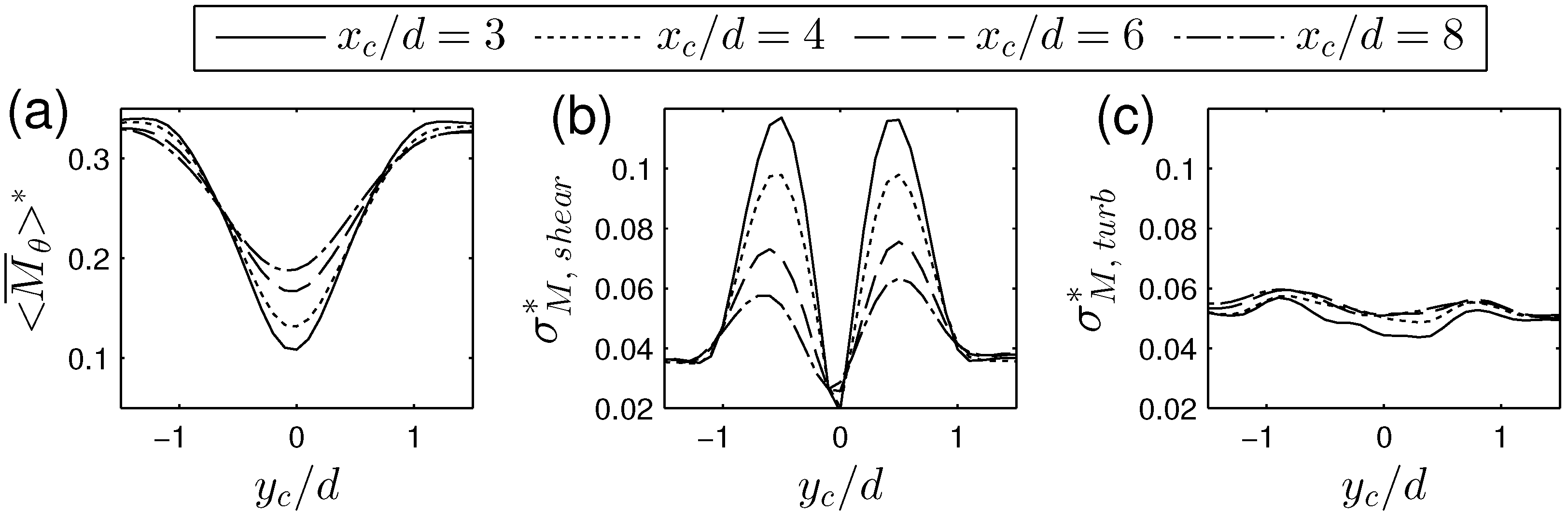
Figure 14a–c shows, respectively, the variation of , and with for different values of . For given and , is the normalized time-space-averaged moment over C. The value of represents moment fluctuations due to mean shear over C. Finally, represents the spatial average of moment fluctuations due to flow turbulent fluctuations.
Based on Figure 14a, for each , is minimum at around . This is expected as C is located in full-wake conditions in this case. With the increase of the magnitude of , the average velocity over C increases which leads to the increase of . Due to the wake growth, one can also observe that increases with for fairly small magnitudes of () and decreases with for large magnitudes of ().
Figure 14b shows that the value of is very sensitive to the relative position of C with respect to the upwind turbine. For the values of around , is maximum as C is located in partial-wake conditions in this case. This means that the blades of the hypothetical turbine located at C experience both the wake flow and the unperturbed outer one at each revolution. Figure 14c shows that the variation of with and is considerably less than that of . In general, we observe that the value of is higher than under full-wake conditions (i.e., ). Under partial-wake conditions, however, is considerably bigger.
The results presented in this section concern the moment of the streamwise momentum flux on the blade root of a hypothetical turbine. Even though this method cannot accurately predict the load bending moments on the blade roots, it is very useful for comparing moment fluctuations due to turbulence and mean shear under different wind-farm layout configurations. It is also worth mentioning that similar analyses can be done in future works for other types of moments acting on the turbine. For instance, the yaw moment of the streamwise momentum flux on the nacelle yaw bearing can be likewise studied.
6. Wake Dynamics: Meandering Motions
One of the most important characteristics of turbine wakes is the meandering motion as it greatly contributes to the unsteadiness of turbine wake flows. Despite its primary importance, the effect of wake meandering on the flow distribution in turbine wakes is not well understood. The S-PIV measurements performed in this paper enabled us to gain insight into how the meandering process affects the cross-section of turbine wakes.
For each instantaneous flow field, the magnitude of wake meandering can be expressed by the displacement of the center of the wake velocity deficit. The instantaneous lateral and vertical positions of the center of the wake velocity deficit, denoted by and respectively, are given by
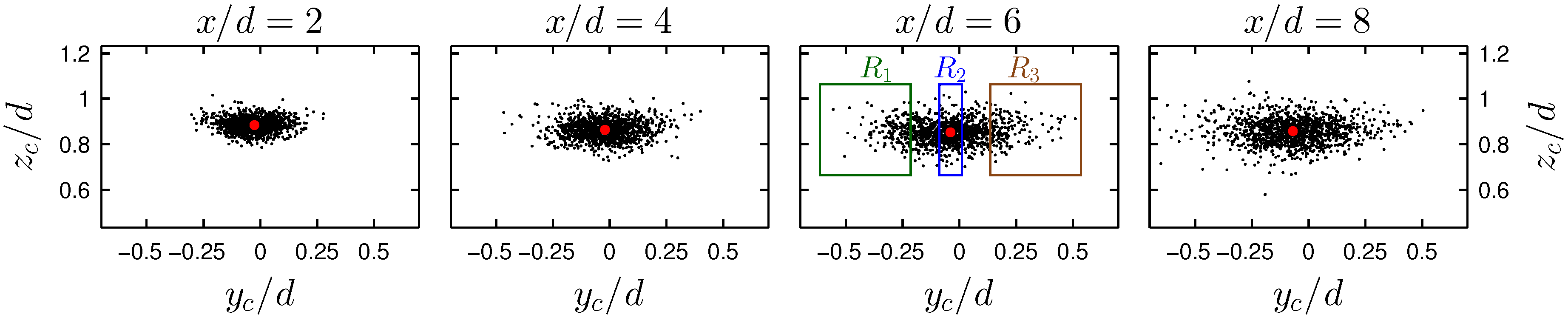
For the sake of brevity, the center of the wake velocity deficit is called wake center in the following. Figure 15 shows the distribution of the wake center position for all the instantaneous flow fields at different downstream locations. As expected, the figure shows that the magnitude of wake meandering increases as the wake moves downstream. The magnitude of wake meandering at different streamwise positions is found to be relatively similar to the one reported in the literature [22,23] for a different miniature turbine. Moreover, one can observe that meandering is significantly more pronounced in the lateral direction with respect to the one in the vertical direction, which is in agreement with prior experimental and numerical studies (e.g., [20,44]). This can be explained by the larger value of with respect to for turbulent boundary layers [20], or the lateral meandering tendency of very-large-scale structures in the incoming boundary layer [45]. The difference of the meandering magnitude in the lateral and vertical directions is also evident in Figure 16, which shows the probability density function (PDF) of the lateral and vertical positions of the wake center at . Moreover, the figure shows that the distribution of the instantaneous wake-center position can be acceptably estimated by a normal distribution. It is also worth mentioning that a normal distribution is found for the distribution of the instantaneous wake-center position at other streamwise positions, and the standard deviation of this normal distribution increases with x.
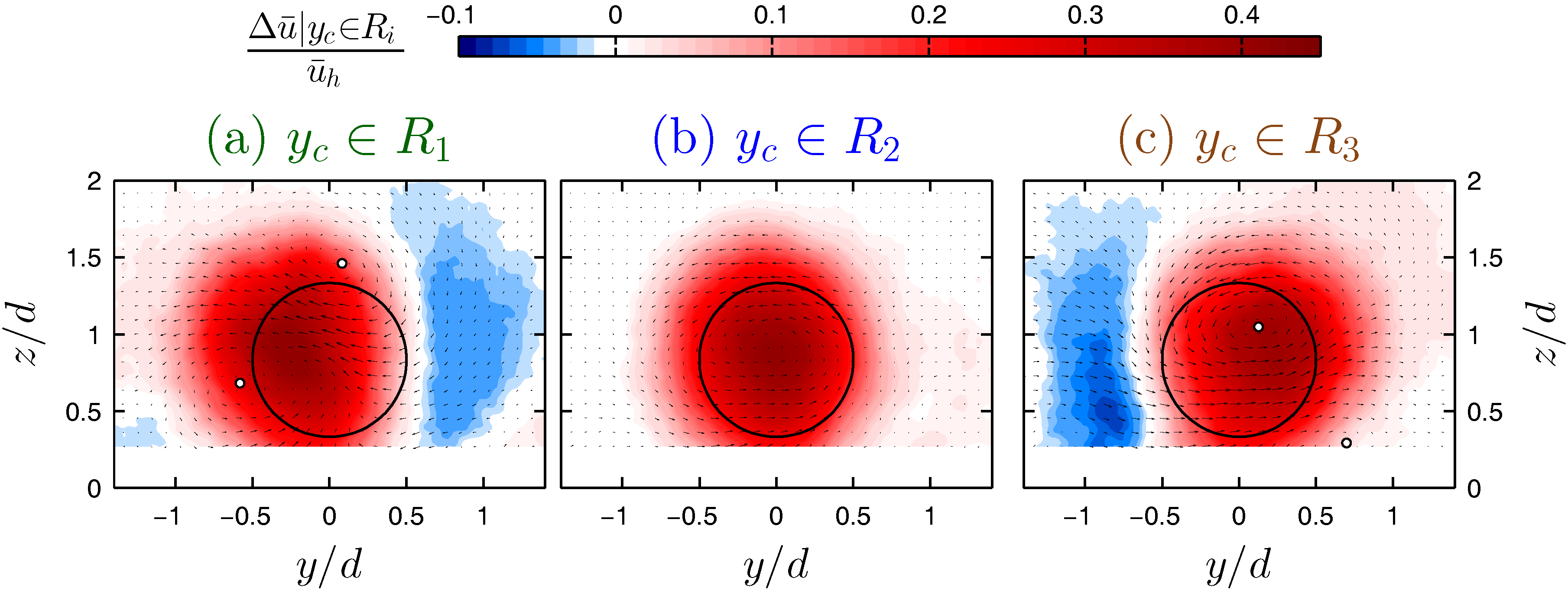
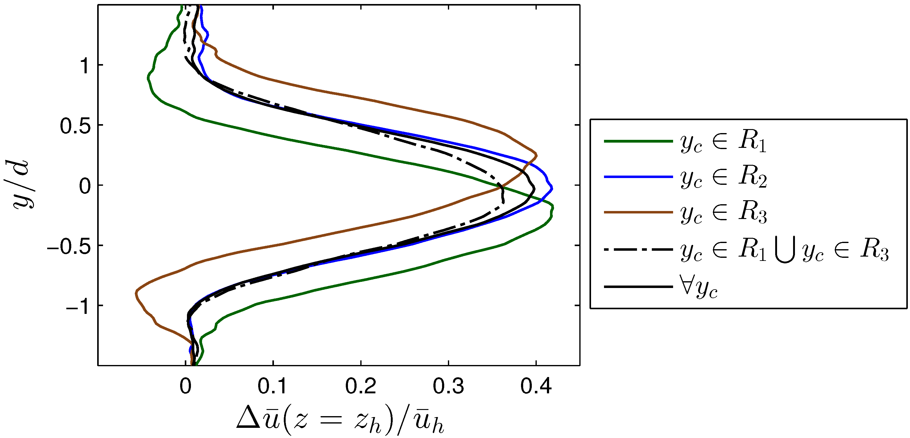
In order to study the effect of this strong lateral meandering tendency on the wake cross-section, conditional averaging is performed on the wake velocity distribution based on the instantaneous position of the wake center. In this regard, three different regions (, and ) are defined in the scatter plot of the wake-center position at in Figure 15. The regions and contain instantaneous flow fields with large lateral meandering motions, while the region contains those with negligible lateral meandering. These regions are selected to be wide enough so that there are at least 150 instantaneous flow fields available for each region. Figure 17 shows contours of the conditionally-averaged normalized velocity deficit at given , where i = 1, 2 and 3, overlaid with vectors of conditionally-averaged in-plane velocity components. In Figure 17a,c, one can observe that the flow has a strong spanwise velocity component, which is due to the lateral displacement of the wake. Moreover, the figure reveals the presence of a counter-rotating vortex pair (CVP) in both of these cases (shown by white dots) although it is more obvious for . It is interesting to mention that this strong lateral velocity with a CVP observed in Figure 17a,c is similar to what occurs for the wake of a yawed turbine, which has been recently reported in Bastankhah and Porté-Agel [18]. The mentioned study stated that the CVP exists in flows with a strong variation of cross-wind velocity to satisfy continuity, which is also the case in Figure 17a,c.
Figure 17a,c also shows that when the wake laterally moves to one side, a high-speed region (i.e., region with a negative velocity deficit) appears on the other side. The existence of the high-speed region in these cases can explain why the mean wake cross-section is not stretched laterally despite large lateral meandering motions. This is more evident in Figure 18 showing lateral profiles of the normalized velocity deficit, at hub height, conditionally averaged based on different positions of . As seen in the figure, cases with large meandering motions (i.e., and ) reduce the effect of each other on laterally expanding the mean wake cross-section due to the presence of these high-speed regions. In fact, the conditionally-averaged velocity-deficit profile given has the same width as the one corresponding to and also the mean normalized velocity deficit profile without any condition (i.e., ). Qualitatively-similar results can be also observed for other streamwise positions although they are not shown here for the sake of brevity.
In order to elucidate the possible origin of the high-speed region observed in Figure 17a,c, one can notice that the flow in both cases is generally directed from the high-speed region to the low-speed one at around turbine hub-height level, and it gradually changes direction with increasing height. This is similar to the flow motion between well-known high- and low-speed streaks, known as very-large-scale motions (VLSMs), in turbulent boundary layers [45,46,47]. In addition, the size of high-speed regions shown in Figure 17a,c is in the same order of magnitude as the values reported in the literature for the size of VLSMs in boundary-layer flows (e.g., [45]). This suggests that the cases and are probably dominated by the interaction of VLSMs with the turbine wake. In other words, what we see in Figure 17a,c is likely to be the superposition of low- and high-speed streaks in the boundary layer with the low-speed rotating wake. This can also explain why the mean width of passive scalar plumes, in contrast to wake flows, is usually bigger than their height (i.e., having an elliptic cross-section) (e.g., [48,49]). In that case, VLSMs do not superimpose on the passive scalar plume simply due to their different natures so that large lateral meandering motions expand the mean plume distribution in the lateral direction, contrary to what we observe for the turbine wake (Figure 18).
This study provides new insights into the effect of wake meandering on the wake cross-section and a possible role of VLSMs in this effect. More research should be performed in the future particularly on the connection between VLSMs and wake meandering.
7. Summary
A new optimized three-bladed miniature wind turbine, called WiRE-01, is designed and fully characterized in Part I of this study [32]. In the current part of the study, the wake structure and flow dynamic characteristics are studied for the new turbine immersed in a turbulent boundary layer. A similarity is found between the spectral density of the thrust force T and the one of at very low-frequency scales. This means that thrust measurements can be used in the field to provide useful information about the incoming flow.
High-resolution S-PIV measurements are carried out to quantify the wake of the miniature turbine and provide a unique dataset for the validation of numerical models. Key information on the wake structure such as velocity and turbulence distributions is presented and discussed in both qualitative and quantitative manners. The results show that the more realistic values of and of the new turbine, compared with previously used miniature turbines, leads to turbine wake flows that have stronger velocity deficit and wake rotation strength.
The wake velocity measurements performed in this study are then used to compare unsteady moments caused by mean shear and turbulence on the blade root of a hypothetical turbine placed downstream. To do so, the moment of the streamwise momentum flux is calculated over a circular area (with the diameter equal to the one of the turbine rotor) placed normal to the flow at different streamwise and lateral positions. The results suggest that, in order to assess moment fluctuations due to turbulence, both mean velocity and velocity turbulent fluctuations should be taken into account. Unlike moment fluctuations due to turbulence, those due to mean shear are found to be very sensitive to the relative position of the downstream hypothetical turbine. A new method is employed to calculate the standard deviation of the moment due to turbulence as well as the one due to mean shear. In general, the former is found to be bigger under full-wake conditions, while the latter is dominant under partial-wake conditions.
In addition, the PIV data are used to study wake meandering and its effect on the wake cross-section. Conditional averaging based on the instantaneous position of the wake center is performed to quantify the wake structure under large meandering motions. Strong spanwise velocity with a CVP is observed in the wake cross-section in this condition, akin to the wake cross-section of yawed turbines. Results also show that when the wake meanders laterally to one side, a high-speed region exists on the opposite side. This high-speed region is the reason that the mean wake cross-section is not stretched laterally despite large meandering motions in the lateral direction. The study also provides insight into the possible connection between the high-speed region and VLSMs in the incoming boundary layer.
Acknowledgments
This research was supported by the Swiss National Science Foundation (grant 200021_172538, and grant 206021_144976), the Swiss Federal Office of Energy (grant SI/501337-01), and the Swiss Innovation and Technology Committee (CTI) within the context of the Swiss Competence Center for Energy Research “FURIES: Future Swiss Electrical Infrastructure”. The first author was also partially supported by the EuroTech Greentech Initiative Wind Energy. The authors would also like to thank Vincent F.C. Rolin for his help on PIV setup preparations.
Author Contributions
This study was done as a part of Majid Bastankhah’s doctoral studies supervised by Fernando Porté-Agel.
Conflicts of Interest
The authors declare no conflict of interest.
References
- Conti, J.; Holtberg, P.; Diefenderfer, J.; LaRose, A. International Energy Outlook 2016; Technical Report; U.S. Energy Information Administration: Washington, DC, USA, 2016.
- Vermeer, L.; Sørensen, J.; Crespo, A. Wind turbine wake aerodynamics. Prog. Aerosp. Sci. 2003, 39, 467–510. [Google Scholar] [CrossRef]
- Sørensen, J.N. Aerodynamic aspects of wind energy conversion. Annu. Rev. Fluid Mech. 2011, 43, 427–448. [Google Scholar] [CrossRef]
- Sanderse, B.; Pijl, S.; Koren, B. Review of computational fluid dynamics for wind turbine wake aerodynamics. Wind Energy 2011, 14, 799–819. [Google Scholar] [CrossRef]
- Mehta, D.; Van Zuijlen, A.; Koren, B.; Holierhoek, J.; Bijl, H. Large eddy simulation of wind farm aerodynamics: A review. J. Wind Eng. Ind. Aerodyn. 2014, 133, 1–17. [Google Scholar] [CrossRef]
- Stevens, R.J.; Meneveau, C. Flow structure and turbulence in wind farms. Annu. Rev. Fluid Mech. 2017, 49, 311–339. [Google Scholar] [CrossRef]
- Medici, D.; Alfredsson, P. Measurement on a wind turbine wake: 3D effects and bluff body vortex shedding. Wind Energy 2006, 9, 219–236. [Google Scholar] [CrossRef]
- Chamorro, L.P.; Porté-Agel, F. A wind-tunnel investigation of wind-turbine wakes: Boundary-layer turbulence effects. Bound. Layer Meteorol. 2009, 132, 129–149. [Google Scholar] [CrossRef]
- Cal, R.B.; Lebrón, J.; Castillo, L.; Kang, H.S.; Meneveau, C. Experimental study of the horizontally averaged flow structure in a model wind-turbine array boundary layer. J. Renew. Sustain. Energy 2010, 2, 013106. [Google Scholar] [CrossRef]
- Chamorro, L.P.; Porté-Agel, F. Effects of thermal stability and incoming boundary-layer flow characteristics on wind-turbine wakes: A wind-tunnel study. Bound. Layer Meteorol. 2010, 136, 515–533. [Google Scholar] [CrossRef]
- Zhang, W.; Markfort, C.D.; Porté-Agel, F. Near-wake flow structure downwind of a wind turbine in a turbulent boundary layer. Exp. Fluids 2012, 52, 1219–1235. [Google Scholar] [CrossRef]
- Markfort, C.; Zhang, W.; Porté-Agel, F. Turbulent flow and scalar transport through and over aligned and staggered wind farms. J. Turbul. 2012, 13, N33. [Google Scholar] [CrossRef]
- Hu, H.; Yang, Z.; Sarkar, P. Dynamic wind loads and wake characteristics of a wind turbine model in an atmospheric boundary layer wind. Exp. Fluids 2012, 52, 1277–1294. [Google Scholar] [CrossRef]
- Zhang, W.; Markfort, C.D.; Porté-Agel, F. Wind-turbine wakes in a convective boundary layer: A wind-tunnel study. Bound. Layer Meteorol. 2013, 146, 161–179. [Google Scholar] [CrossRef]
- Iungo, G.V.; Viola, F.; Camarri, S.; Porté-Agel, F.; Gallaire, F. Linear stability analysis of wind turbine wakes performed on wind tunnel measurements. J. Fluid Mech. 2013, 737, 499–526. [Google Scholar] [CrossRef]
- Hancock, P.; Pascheke, F. Wind-tunnel simulation of the wake of a large wind turbine in a stable boundary layer: Part 2, the wake flow. Bound. Layer Meteorol. 2014, 151, 23–37. [Google Scholar] [CrossRef]
- Bastankhah, M.; Porté-Agel, F. A wind-tunnel investigation of wind-turbine wakes in yawed conditions. J. Phys. Conf. Ser. 2015, 625, 012014. [Google Scholar] [CrossRef]
- Bastankhah, M.; Porté-Agel, F. Experimental and theoretical study of wind turbine wakes in yawed conditions. J. Fluid Mech. 2016, 806, 506–541. [Google Scholar] [CrossRef]
- Bastankhah, M.; Porté-Agel, F. Wind tunnel study of the wind turbine interaction with a boundary-layer flow: Upwind region, turbine performance, and wake region. Phys. Fluids 2017, 29, 065105. [Google Scholar] [CrossRef]
- España, G.; Aubrun, S.; Loyer, S.; Devinant, P. Spatial study of the wake meandering using modelled wind turbines in a wind tunnel. Wind Energy 2011, 14, 923–937. [Google Scholar] [CrossRef]
- España, G.; Aubrun, S.; Loyer, S.; Devinant, P. Wind tunnel study of the wake meandering downstream of a modelled wind turbine as an effect of large scale turbulent eddies. J. Wind Eng. Ind. Aerodyn. 2012, 101, 24–33. [Google Scholar] [CrossRef]
- Howard, K.B.; Singh, A.; Sotiropoulos, F.; Guala, M. On the statistics of wind turbine wake meandering: An experimental investigation. Phys. Fluids 2015, 27, 075103. [Google Scholar] [CrossRef]
- Foti, D.; Yang, X.; Guala, M.; Sotiropoulos, F. Wake meandering statistics of a model wind turbine: Insights gained by large eddy simulations. Phys. Rev. Fluids 2016, 1, 044407. [Google Scholar] [CrossRef]
- Barthelmie, R.J.; Frandsen, S.T.; Nielsen, M.; Pryor, S.; Rethore, P.E.; Jørgensen, H.E. Modelling and measurements of power losses and turbulence intensity in wind turbine wakes at Middelgrunden offshore wind farm. Wind Energy 2007, 10, 517–528. [Google Scholar] [CrossRef]
- Porté-Agel, F.; Wu, Y.T.; Lu, H.; Conzemius, R.J. Large-eddy simulation of atmospheric boundary layer flow through wind turbines and wind farms. J. Wind Eng. Ind. Aerodyn. 2011, 99, 154–168. [Google Scholar] [CrossRef]
- Chamorro, L.P.; Porté-Agel, F. Turbulent flow inside and above a wind farm: A wind-tunnel study. Energies 2011, 4, 1916–1936. [Google Scholar] [CrossRef]
- Meyers, J.; Meneveau, C. Optimal turbine spacing in fully developed wind farm boundary layers. Wind Energy 2012, 15, 305–317. [Google Scholar] [CrossRef]
- Porté-Agel, F.; Wu, Y.T.; Chen, C.H. A numerical study of the effects of wind direction on turbine wakes and power losses in a large wind farm. Energies 2013, 6, 5297–5313. [Google Scholar] [CrossRef]
- Wu, Y.; Porté-Agel, F. Large-eddy simulation of wind-turbine wakes: Evaluation of turbine parametrisations. Bound. Layer Meterol. 2011, 138, 345–366. [Google Scholar] [CrossRef]
- Xie, S.; Archer, C. Self-similarity and turbulence characteristics of wind turbine wakes via large-eddy simulation. Wind Energy 2015, 18, 1815–1838. [Google Scholar] [CrossRef]
- Bastankhah, M.; Porté-Agel, F. A new analytical model for wind-turbine wakes. Renew. Energy 2014, 70, 116–123. [Google Scholar] [CrossRef]
- Bastankhah, M.; Porté-Agel, F. A new miniature wind turbine for wind tunnel experiments. Part I: Design and performance. Energies 2017, 10, 908. [Google Scholar] [CrossRef]
- Garratt, J.R. Review: the atmospheric boundary layer. Earth Sci. Rev. 1994, 37, 89–134. [Google Scholar] [CrossRef]
- Bottasso, C.; Cacciola, S.; Schreiber, J. A wake detector for wind farm control. J. Phys. Conf. Ser. 2015, 625, 012007. [Google Scholar] [CrossRef]
- Cacciola, S.; Bertelè, M.; Bottasso, C. Simultaneous observation of wind shears and misalignments from rotor loads. J. Phys. Conf. Ser. 2016, 753, 052002. [Google Scholar] [CrossRef]
- Scheffer, C.; Girdhar, P. Practical Machinery Vibration Analysis and Predictive Maintenance; Elsevier: Burlington, MA, USA, 2004. [Google Scholar]
- De Silva, C.W. Vibration Monitoring, Testing, and Instrumentation; CRC Press: Boca Raton, FL, USA, 2007. [Google Scholar]
- Yang, Z.; Sarkar, P.; Hu, H. Visualization of the tip vortices in a wind turbine wake. J. Vis. 2012, 15, 39–44. [Google Scholar] [CrossRef]
- Lignarolo, L.; Ragni, D.; Krishnaswami, C.; Chen, Q.; Simao Ferreira, C.; van Bussel, G. Experimental analysis of the kinetic energy transport and turbulence production in the wake of a model wind turbine. In Proceedings of the ICOWES Conference, Lyngby, Denmark, 17–19 June 2013; pp. 16–19. [Google Scholar]
- Stull, R.B. An Introduction to Boundary Layer Meteorology; Springer Science: Berlin, Germany, 2009; Volume 13. [Google Scholar]
- Shamsoddin, S.; Porté-Agel, F. A large-eddy simulation study of vertical axis wind turbine wakes in the atmospheric boundary layer. Energies 2016, 9, 366. [Google Scholar] [CrossRef]
- Frandsen, S.T. Turbulence and Turbulence-Generated Structural Loading in Wind Turbine Clusters. Ph.D. Thesis, Risø National Laboratoy, Roskilde, Denmark, 2007. [Google Scholar]
- Wu, Y.; Porté-Agel, F. Atmospheric turbulence effects on wind-turbine wakes: An LES study. Energies 2012, 5, 5340–5362. [Google Scholar] [CrossRef]
- Abkar, M.; Porté-Agel, F. Influence of atmospheric stability on wind-turbine wakes: A large-eddy simulation study. Phys. Fluids 2015, 27, 035104. [Google Scholar] [CrossRef]
- Hutchins, N.; Marusic, I. Evidence of very long meandering features in the logarithmic region of turbulent boundary layers. J. Fluid Mech. 2007, 579, 1–28. [Google Scholar] [CrossRef]
- Hutchins, N.; Chauhan, K.; Marusic, I.; Monty, J.; Klewicki, J. Towards reconciling the large-scale structure of turbulent boundary layers in the atmosphere and laboratory. Bound. Layer Meteorol. 2012, 145, 273–306. [Google Scholar] [CrossRef]
- Fang, J.; Porté-Agel, F. Large-Eddy Simulation of Very-Large-Scale Motions in the Neutrally Stratified Atmospheric Boundary Layer. Bound. Layer Meteorol. 2015, 155, 397–416. [Google Scholar] [CrossRef]
- Fackrell, J.; Robins, A. Concentration fluctuations and fluxes in plumes from point sources in a turbulent boundary layer. J. Fluid Mech. 1982, 117, 1–26. [Google Scholar] [CrossRef]
- Nironi, C.; Salizzoni, P.; Marro, M.; Mejean, P.; Grosjean, N.; Soulhac, L. Dispersion of a passive scalar fluctuating plume in a turbulent boundary layer. Part I: Velocity and concentration measurements. Bound. Layer Meteorol. 2015, 156, 415–446. [Google Scholar] [CrossRef]
Figure 1.
(a) Schematic figure of the miniature wind turbine placed in the turbulent boundary layer. (b) Variation of and with the tip-speed ratio for the miniature turbine placed in the boundary layer with ms.
Figure 1.
(a) Schematic figure of the miniature wind turbine placed in the turbulent boundary layer. (b) Variation of and with the tip-speed ratio for the miniature turbine placed in the boundary layer with ms.
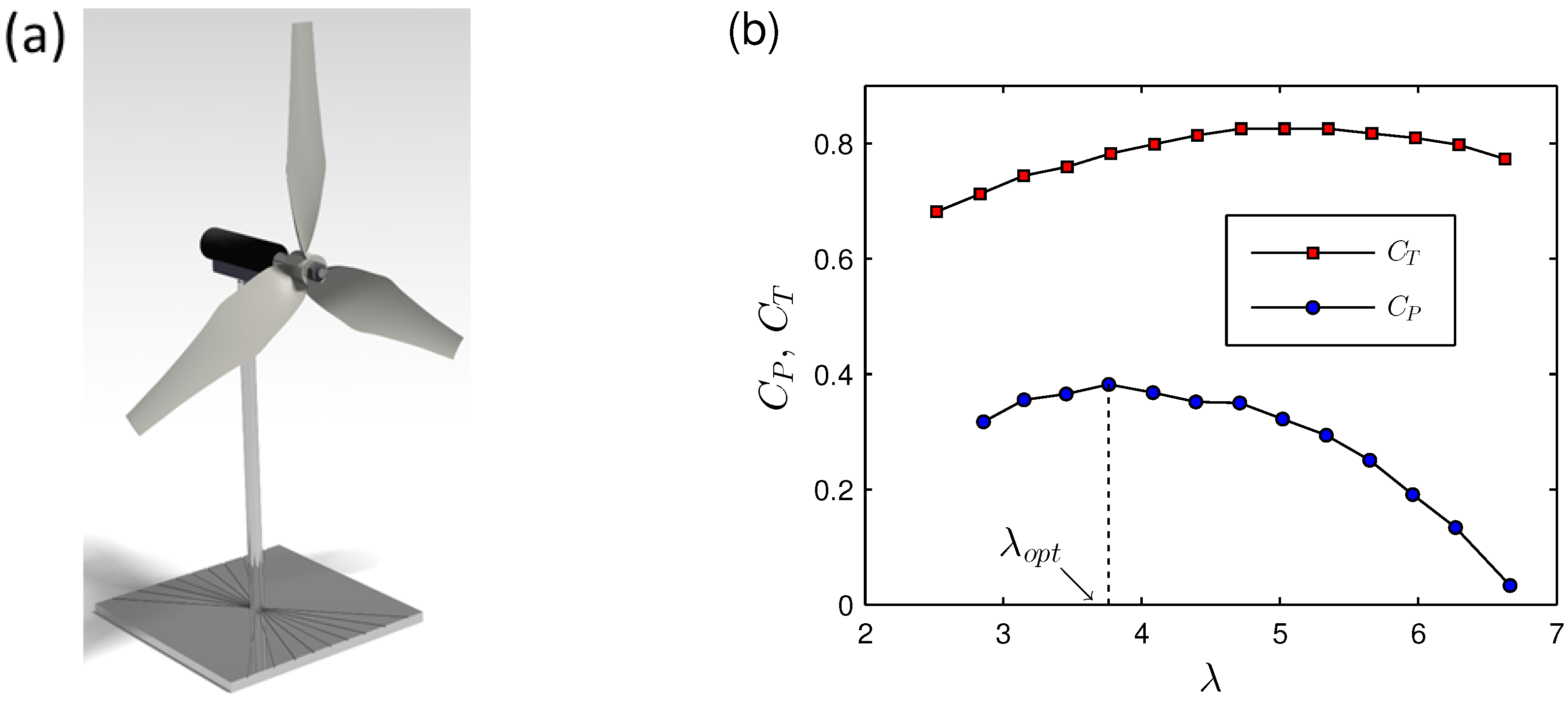
Figure 2.
Characteristics of the incoming boundary layer: (a) normalized mean velocity and (b) turbulence intensity, obtained with a single hot-wire anemometer. The dashed and solid lines represent the turbine axis and fitted power-law curve, respectively. (c) Normalized vertical turbulent momentum flux, obtained with a stereo particle image-velocimetry (S-PIV) system.
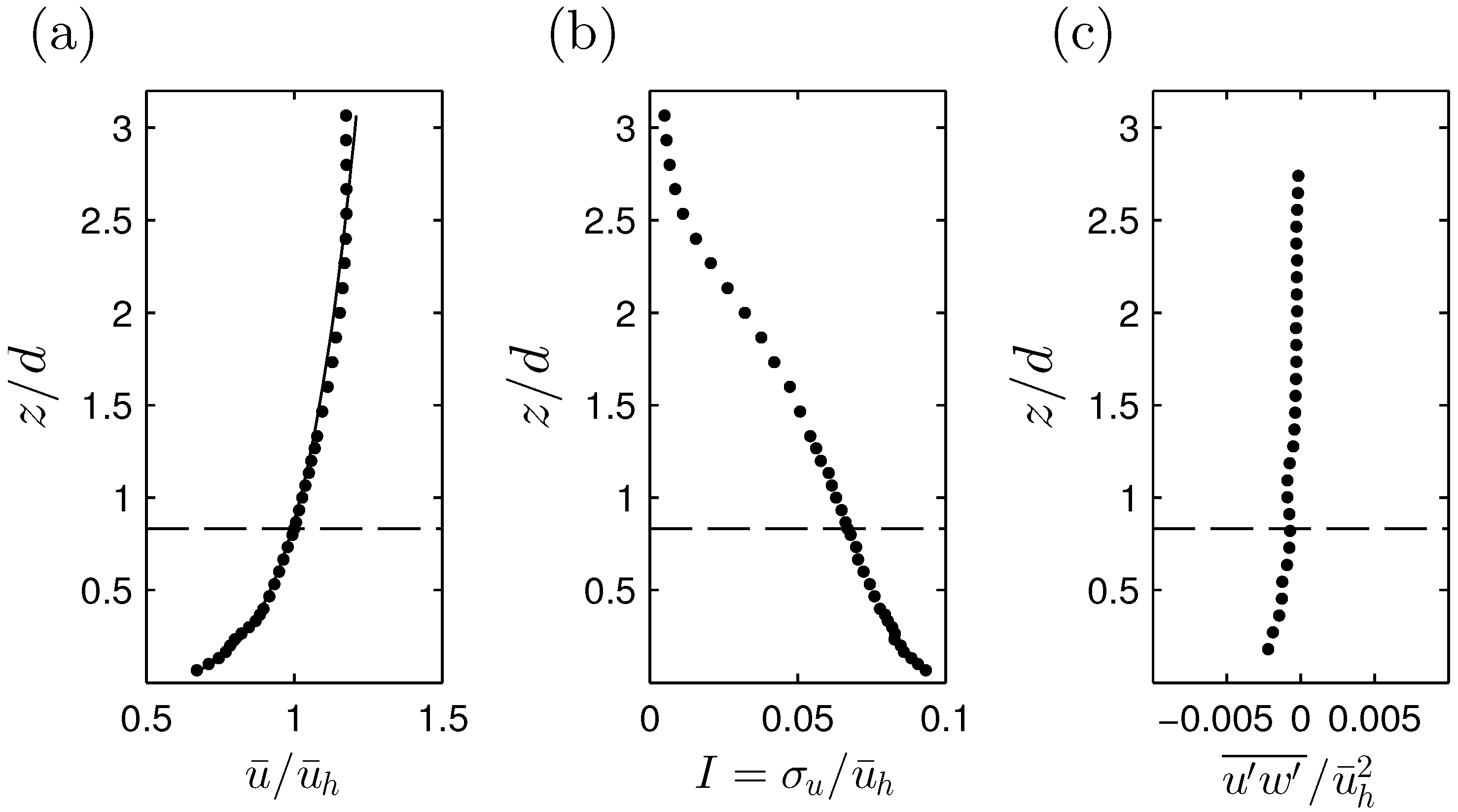
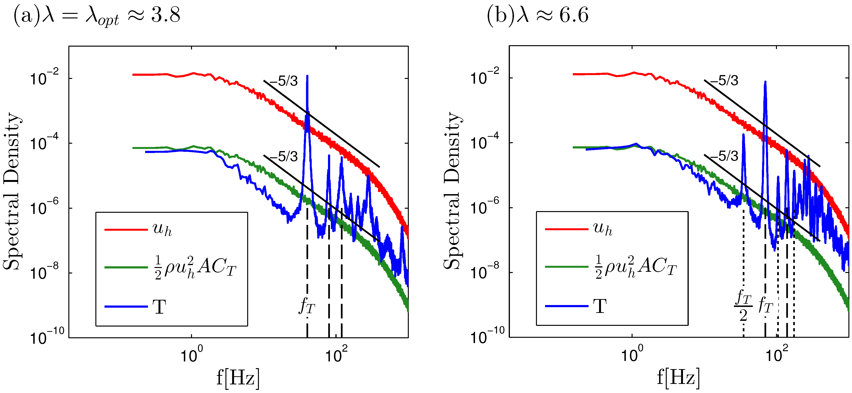
Figure 3.
Spectral density of the incoming velocity at hub height , the thrust force T and for two different tip-speed ratios. The rotational frequency of the rotor and its harmonics are shown by dashed lines. One half of the rotor rotational frequency and its harmonics are shown by dotted lines.
Figure 3.
Spectral density of the incoming velocity at hub height , the thrust force T and for two different tip-speed ratios. The rotational frequency of the rotor and its harmonics are shown by dashed lines. One half of the rotor rotational frequency and its harmonics are shown by dotted lines.

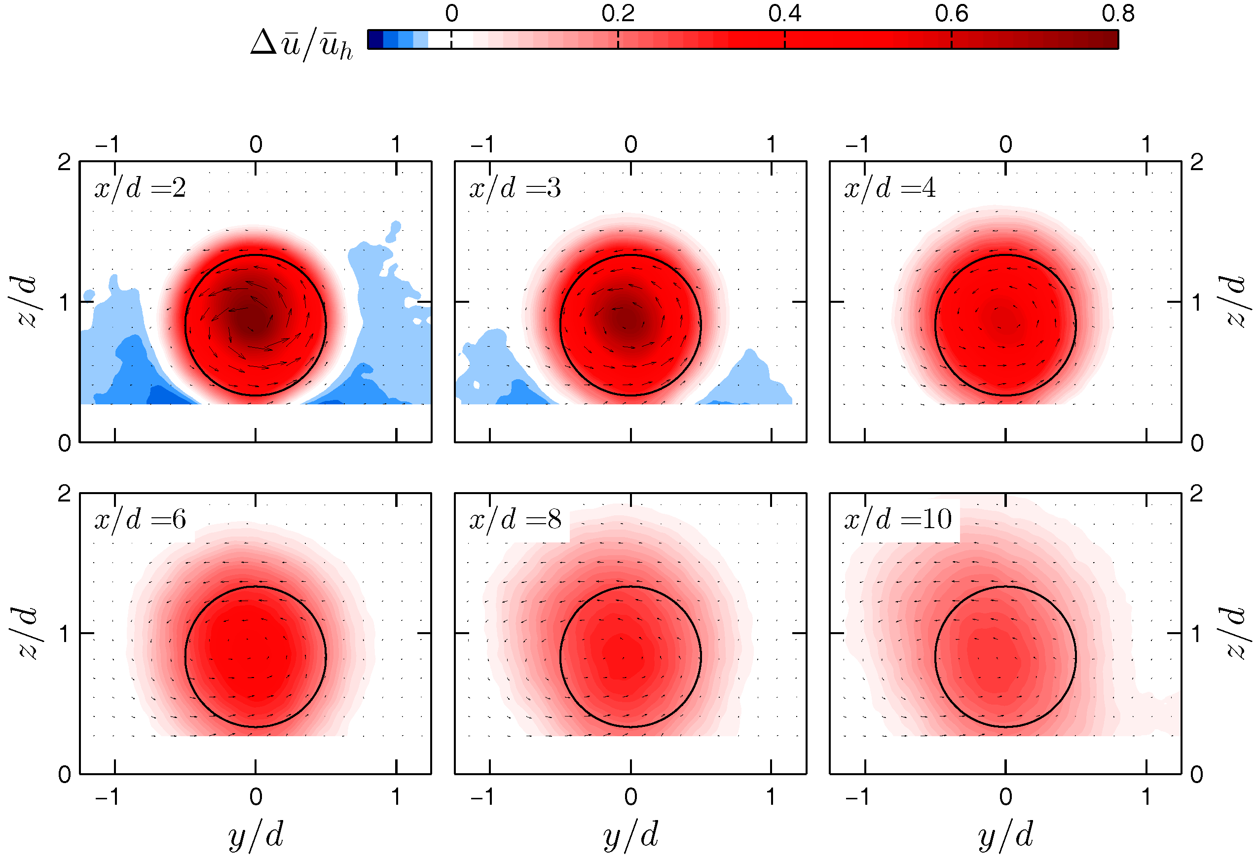
Figure 4.
Contours of the normalized velocity deficit in planes at different downstream locations for the miniature turbine operating at . The vector field represents the in-plane velocity components. The black circles show the frontal area of the wind turbine.
Figure 4.
Contours of the normalized velocity deficit in planes at different downstream locations for the miniature turbine operating at . The vector field represents the in-plane velocity components. The black circles show the frontal area of the wind turbine.

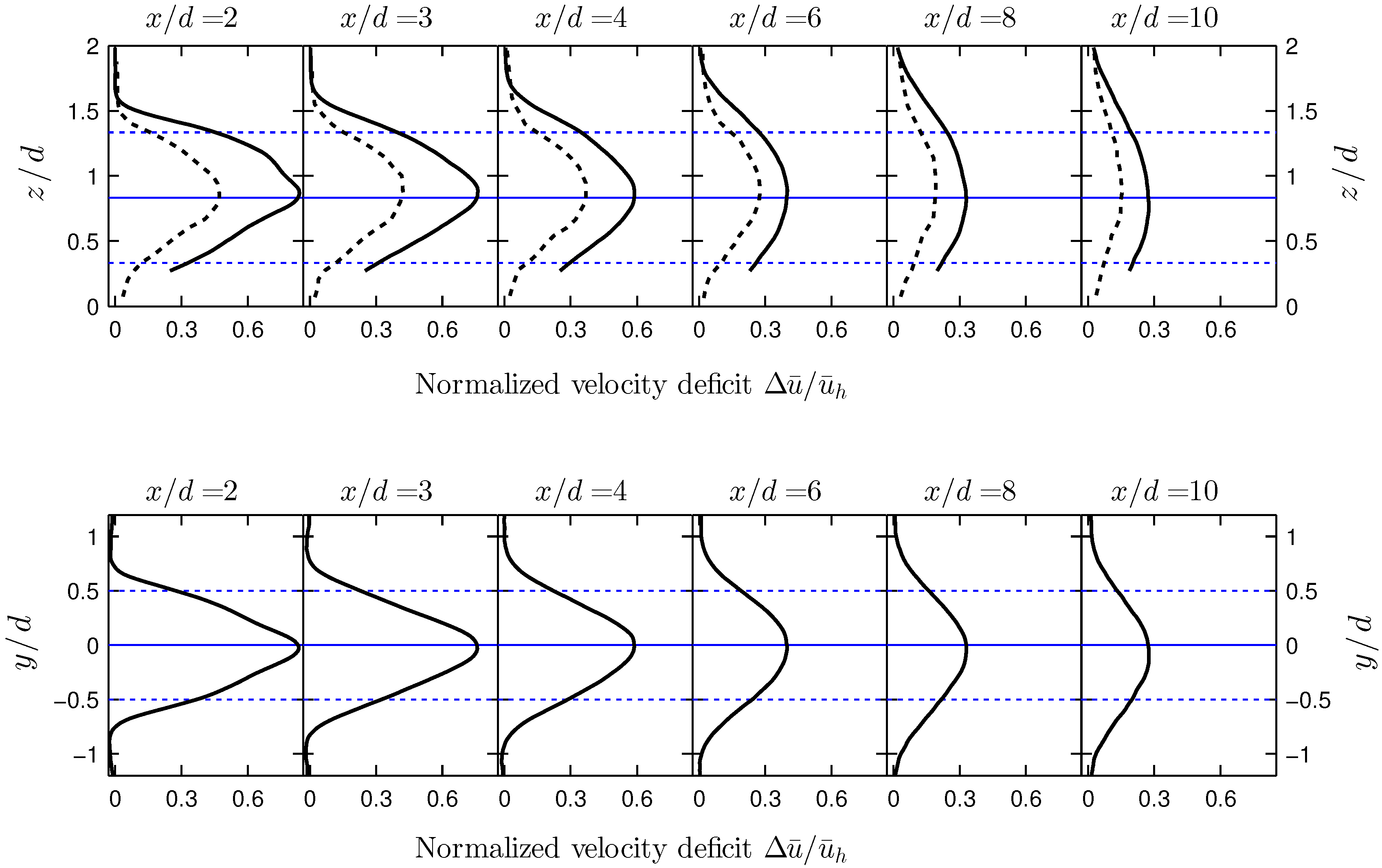
Figure 5.
Vertical (top) and lateral (bottom) profiles of the normalized velocity deficit through the hub level at different downstream locations. Solid black lines: new miniature turbine, and dashed black lines: Chamorro and Porté-Agel [10]. Blue solid lines and blue dashed lines represent the rotor axis and the tip positions, respectively.

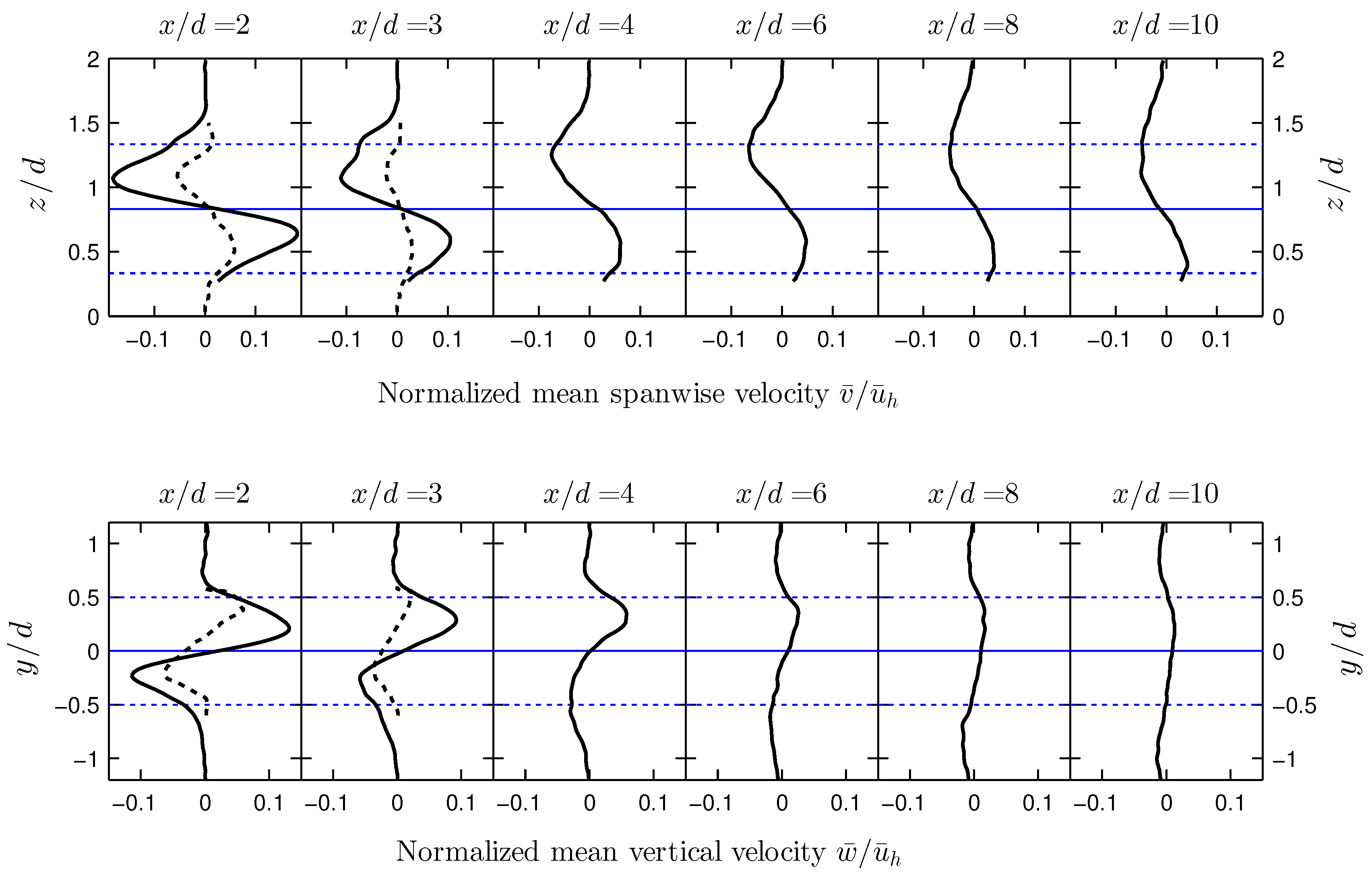
Figure 6.
Vertical profiles of the normalized spanwise velocity (top) and lateral profiles of the normalized vertical velocity (bottom) through the hub level at different downstream locations. Solid black lines: new miniature turbine, and dashed black lines: Zhang et al. [11]. Blue solid lines and blue dashed lines represent the rotor axis and the tip positions, respectively.

Figure 7.
Contours of the normalized vertical momentum turbulent flux in planes at different downstream locations for the miniature turbine operating at . The vector field represents the in-plane velocity components. The black circles show the frontal area of the wind turbine.
Figure 7.
Contours of the normalized vertical momentum turbulent flux in planes at different downstream locations for the miniature turbine operating at . The vector field represents the in-plane velocity components. The black circles show the frontal area of the wind turbine.
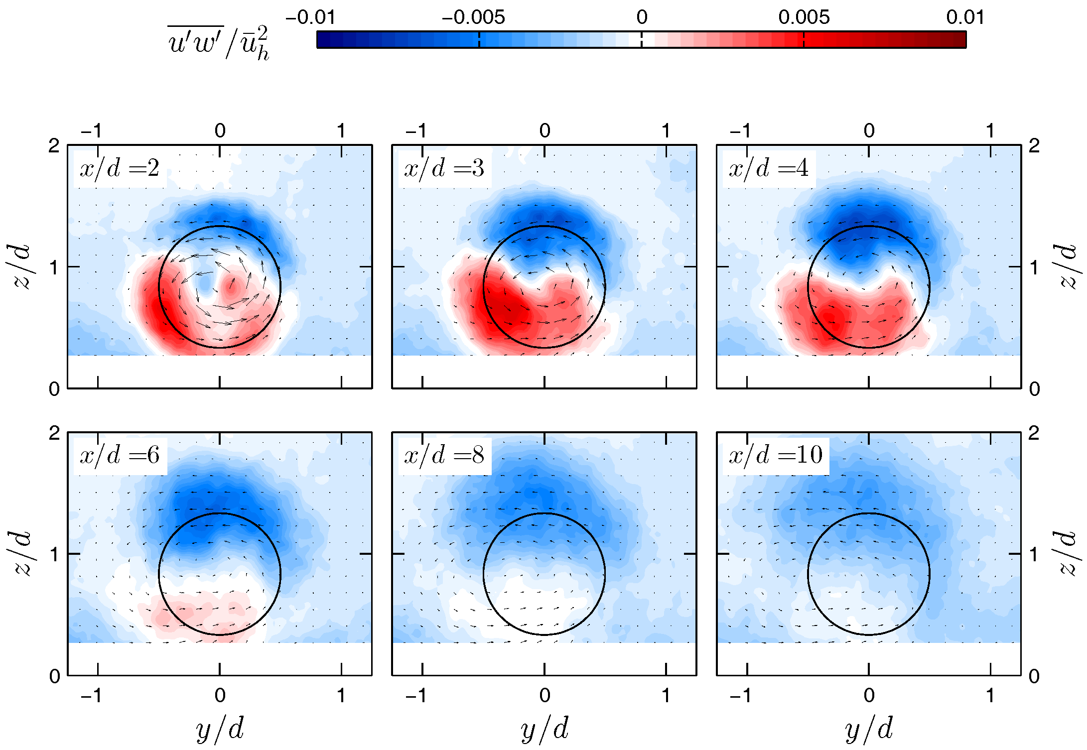
Figure 8.
Contours of the normalized lateral momentum turbulent flux in planes at different downstream locations for the miniature turbine operating at . The vector field represents the in-plane velocity components. The black circles show the frontal area of the wind turbine.
Figure 8.
Contours of the normalized lateral momentum turbulent flux in planes at different downstream locations for the miniature turbine operating at . The vector field represents the in-plane velocity components. The black circles show the frontal area of the wind turbine.

Figure 9.
Vertical profiles of the normalized vertical momentum turbulent flux (top) and lateral profiles of the normalized lateral momentum turbulent flux (bottom) at hub level at different downstream locations. Blue solid lines and blue dashed lines represent the rotor axis and the tip positions, respectively.

Figure 10.
Contours of the added streamwise turbulence intensity in planes at different downstream locations for the miniature turbine operating at . The vector field represents the in-plane velocity components. The black circles show the frontal area of the wind turbine.
Figure 10.
Contours of the added streamwise turbulence intensity in planes at different downstream locations for the miniature turbine operating at . The vector field represents the in-plane velocity components. The black circles show the frontal area of the wind turbine.

Figure 11.
Vertical (top) and lateral (bottom) profiles of the added streamwise turbulence intensity at hub level at different downstream locations. Blue solid lines and blue dashed lines represent the rotor axis and the tip positions, respectively.
Figure 11.
Vertical (top) and lateral (bottom) profiles of the added streamwise turbulence intensity at hub level at different downstream locations. Blue solid lines and blue dashed lines represent the rotor axis and the tip positions, respectively.

Figure 12.
Schematic of the circular plane C where a hypothetical downstream turbine is located.

Figure 13.
(a–e) Variation of with the azimuthal angle for different values of at . Error bars also indicate the value of non-dimensionalized with . (f) The ratio of to for different azimuthal angles at and . The azimuthal angle is zero along the positive z-axis, and it increases towards the positive y-axis.

Figure 14.
Variation of (a) , (b) and (c) with for different values of .

Figure 15.
Scatter plot of the instantaneous wake-center position at different downstream locations. The red dots indicate the mean value of the wake-center position at each downstream location. Rectangles , and are used to perform conditional averaging shown in Figure 17.
Figure 15.
Scatter plot of the instantaneous wake-center position at different downstream locations. The red dots indicate the mean value of the wake-center position at each downstream location. Rectangles , and are used to perform conditional averaging shown in Figure 17.

Figure 16.
Probability density function (PDF) of the wake-center position in both lateral and vertical directions at . The blue curves show the fitted normal distributions.
Figure 16.
Probability density function (PDF) of the wake-center position in both lateral and vertical directions at . The blue curves show the fitted normal distributions.
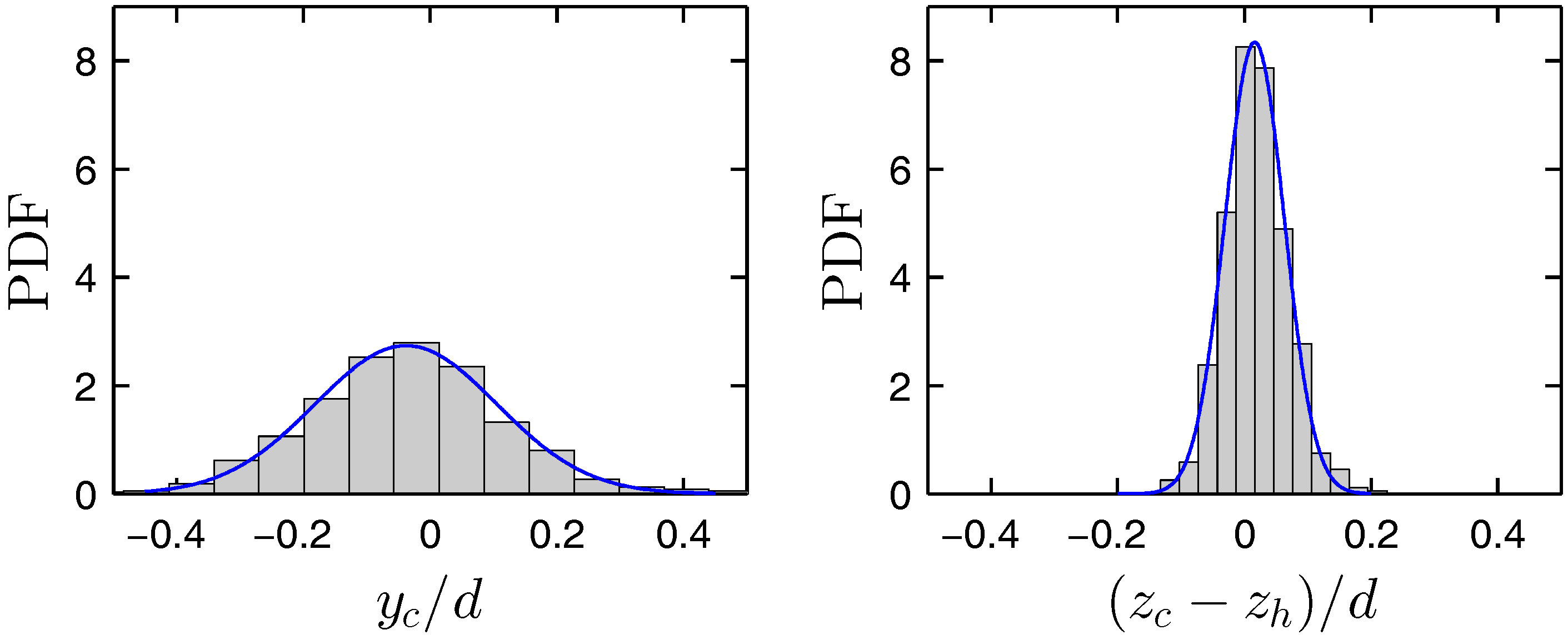
Figure 17.
Contours of the conditionally-averaged normalized velocity deficit at for: (a) , (b) and (c) . The vector field represents conditionally-averaged in-plane velocity components. Black circles indicate the frontal area of the wind turbine. White dots show the approximate position of the counter-rotating vortex pair (CVP).

Figure 18.
Lateral profiles of the normalized velocity deficit at hub height conditionally averaged based on different positions of at .
Figure 18.
Lateral profiles of the normalized velocity deficit at hub height conditionally averaged based on different positions of at .
© 2017 by the authors. Licensee MDPI, Basel, Switzerland. This article is an open access article distributed under the terms and conditions of the Creative Commons Attribution (CC BY) license (http://creativecommons.org/licenses/by/4.0/).
Share and Cite
MDPI and ACS Style
Bastankhah, M.; Porté-Agel, F. A New Miniature Wind Turbine for Wind Tunnel Experiments. Part II: Wake Structure and Flow Dynamics. Energies 2017, 10, 923. https://doi.org/10.3390/en10070923
AMA Style
Bastankhah M, Porté-Agel F. A New Miniature Wind Turbine for Wind Tunnel Experiments. Part II: Wake Structure and Flow Dynamics. Energies. 2017; 10(7):923. https://doi.org/10.3390/en10070923
Chicago/Turabian StyleBastankhah, Majid, and Fernando Porté-Agel. 2017. "A New Miniature Wind Turbine for Wind Tunnel Experiments. Part II: Wake Structure and Flow Dynamics" Energies 10, no. 7: 923. https://doi.org/10.3390/en10070923
Note that from the first issue of 2016, this journal uses article numbers instead of page numbers. See further details here.