
Integration of Degradation Processes in a Strategic Offshore Wind Farm O&M Simulation Model


SINTEF Energy Research, Department of Energy Systems, Trondheim 7465, Norway
*
Author to whom correspondence should be addressed.
Energies 2017, 10(7), 925; https://doi.org/10.3390/en10070925
Submission received: 28 April 2017
/
Revised: 25 June 2017
/
Accepted: 29 June 2017
/
Published: 4 July 2017
(This article belongs to the Special Issue Wind Turbine 2017)
Abstract
:Decision support models for offshore wind farm operation and maintenance (O&M) are required to represent the failure behavior of wind turbine components. Detailed degradation modelling is already incorporated in models for specific components and applications. However, component degradation is only one of many effects that must be captured in high-level strategic decision support models that simulate entire wind farms. Thus, for practical applications, a trade-off is needed between detailed degradation modelling and the level of simplicity of input data representation. To this end, this paper discusses two alternative approaches for taking into account component degradation processes in strategic offshore wind farm O&M simulation models: (1) full integration of the degradation process in the O&M simulation model; and (2) loose integration where the degradation process is translated into simplified input to the O&M model. As a proof-of-concept, a Markov process for blade degradation has been considered. Simulations using the NOWIcob O&M model show that the difference between full and loose integration is small in terms of aggregated output parameters such as average wind turbine availability and O&M costs. Although loose integration models some effects less accurately than full integration, the former is more flexible and convenient, and the accuracy is for most purposes sufficient for such O&M models.
1. Introduction
In order to make offshore wind power competitive with other energy sources, the cost of offshore wind power, i.e., the levelized cost of energy (LCOE) for offshore wind farms, must be reduced. For offshore wind farms, operational expenditures (OPEX) are major contributors to the LCOE, with estimates of this contribution varying from 12–32%, depending on the parameters included in the OPEX [1]. Thus, substantial LCOE reductions will be difficult to achieve without making offshore wind farm operation and maintenance (O&M) more cost-effective.
One potential means of achieving O&M cost reductions is to identify improved O&M and logistics strategies, such as the selection of optimal vessel fleets for carrying out offshore wind farm O&M and investment in cost-effective O&M concepts (e.g., procurement of improved condition monitoring systems). Offshore wind farm O&M models and decision support tools (henceforth referred to as O&M models) are used to assess the economic viability of a wind farm and can assist in evaluations of alternative O&M strategies with the aim of identifying those that are optimal and cost-effective. Such models are thus effective tools in the decision-making process.
A large number of different O&M models have been developed during the last 10–15 years, and reviews carried out by Hofmann [2] and Shafiee [3] provide an overview of these models. Shafiee [3] divides O&M and logistics models into the categories strategic, tactical and operational, depending on the time scale of the decision problem they address. Operational decisions, such as which turbine to visit the next day, have a typical time-horizon of one or a few days. Tactical decisions, such as when to charter a jack-up vessel for a maintenance campaign, have a typical time horizon of several weeks or months, and up to one or two years. Strategic decisions, such as those regarding the optimal vessel fleet for O&M of an offshore wind farm, have a typical time horizon of several years or the wind farm's entire lifetime. Furthermore, models can broadly be subdivided into optimization and simulation models, where the former use mathematical optimization techniques to find an optimal solution, and the latter run simulations of a given set of solution alternatives.
This paper focuses on simulation models that support strategic decisions. Examples of such models include the ECN (Energy Research Centre of the Netherlands) O&M Calculator [4], EDF's (Électricité de France) ECUME model [5], the Strathclyde University offshore wind OPEX model [6] and NOWIcob (Norwegian offshore wind power life cycle cost and benefit) model [7]. The last of these has been used as a basis for the analysis presented in this paper. The aforementioned tools simulate the operational phase of offshore wind farms with the aim of estimating aggregated result parameters, such as O&M costs and average wind turbine availability. To achieve this, they must capture operational factors such as weather conditions, offshore logistics and maintenance activities for all turbines and components in the wind farm.
The extent of maintenance activities carried out at an offshore wind farm depends on the degradation of wind turbine components and their rates of failure. Most O&M models, such as those mentioned above, use only a high-level representation of turbine or component failure behavior [8]. Typically, failure behavior is described in terms of failure rates, which may either be constant or varying over time. However, the use of more detailed models for component failure behavior may improve O&M models and their results. Explicit modelling of the interactions between component degradation, maintenance actions and failures would assist in evaluating the effect of new and advanced inspection technologies or strategies on the number of maintenance actions and failure rates. For example, the introduction of a new and better inspection method may increase the probability of detecting incipient failures and at the same time increase the pre-warning time. Such effects can be modelled by, for example, using a degradation model instead of a failure rate model.
Full integration of degradation processes in an O&M model requires changes in the model’s source code, such as replacement of a conventional, simplified failure rate model with a more advanced, and more complex, degradation model. This increase in O&M model complexity may increase the computational time for simulations. Thus, for practical application and ease of use, a trade-off is required between detailed degradation modelling and the simplicity of the models.
Full integration is usually not a feasible approach for model users, because the source code of most O&M models is not accessible to the end user. Thus, alternative approaches, such as the “loose integration” approach presented and evaluated in this paper, are potentially very useful. This approach allows users to add new features that are not initially included in an O&M model, without requiring changes to the model itself. The approach may also be of interest to model developers since it avoids over-complexity and time-consuming development processes for very specific and occasional model applications.
Obviously, simplified integration alternatives, such as the loose integration approach presented here, should be evaluated in terms of their suitability for the intended purpose. Thus, the aims of this paper are to evaluate the value of more detailed modelling and to discuss the two alternatives for degradation model integration; namely full and loose integration. The main contribution of this paper is thus to present a simple and flexible approach to the representation of degradation and condition-based maintenance in O&M models and to demonstrate that this approach can, in spite of its simplicity, be perfectly adequate in many situations.
Degradation models and offshore wind farm O&M and logistics models have already been the subject of a large number of studies and publications. This is illustrated in Section 2, which addresses degradation and maintenance modelling and by the O&M model examples listed above and in [8,9,10,11]. Previous studies have not considered the integration of degradation models in strategic O&M simulation models, with the exception of a recent paper by Florian and Sørensen [12]. However, this study does not discuss different integration alternatives. In contrast, the present paper sets out and discusses two integration approaches, using a similar case study to that employed in [12]. It also presents a broader discussion of the implications of different approaches to modelling degradation and condition-based maintenance.
The two integration approaches are described in detail in Section 3. A case study has been carried out (Section 4) to show the difference between full and loose integration, identify advantages and disadvantages and provide recommendations on the use of the respective approaches. The results show that the difference between full and loose integration in terms of aggregated result parameters such as availability and O&M costs are small. As discussed in Section 5, and summarized in Section 6, we argue that the accuracy of loose integration is adequate for many O&M model applications. In other words, we find that the detailed modelling of component degradation combined with weather conditions and offshore logistics is of limited value for such applications. However, for applications such as providing decision support for the optimization of inspection strategies, the somewhat greater accuracy of full integration may be an advantage. The benefits of loose integration are its ease of implementation and its flexibility with respect to input data availability regarding the degradation and failure behavior of wind turbine components.
2. Degradation and Maintenance Modelling
Degradation is described as a “detrimental change in ability to meet requirements” [13]. Furthermore, “degradation beyond specified limits may constitute a degraded state or failure” [13]. Note that a degraded state does not mean that a component has failed, but represents a “state of reduced ability to perform as required, but with acceptable reduced performance” [13]. However, a degraded state is sometimes called incipient failure because sooner or later, further degradation will lead to failure.
Degradation is also referred to as deterioration, and serious degradation/deterioration implies poor technical condition and a degraded state “close” to failure. The terms condition, deterioration and degradation are thus often interchangeable.
In situations where degradation can be measured, for instance by means of inspections or condition monitoring, and the measured data combined with a suitable degradation model, it is possible to estimate the remaining time to failure. Furthermore, the effect of preventive maintenance (PM) and corrective maintenance (CM) can be described as an improvement in technical condition to a less degraded state. Degradation models thus offer powerful means of describing and modelling the effects of inspections and maintenance on remaining lifetime and failure probability. Consequently, the use of degradation models in offshore wind farm O&M models has the potential to improve the capabilities and levels of detail of the O&M models.
Degradation can be modelled in different ways. Common to most models is the implication that degradation can be described or represented by an observable variable such as a direct measure of a physical degradation process (e.g., the length of a crack), an indirect measure related to product performance (e.g., the power of a motor) or a qualitative measure as assessed by maintenance personnel (e.g., condition states such as “good”, “minor degradation”, “major degradation”, etc.). Even though a single degradation variable is used in most models, cases involving several underlying degradation processes may require the use of more than one degradation variable. Time is often used as the measure of usage in degradation models. However, other quantities such as the number of revolutions or number of operations may be more suitable in some cases [14]. Based on [15], degradation models can be classified into (1) physical (or physics-based) models; (2) stochastic models and (3) data-driven models/computational intelligence (CI). Physical models, data-driven models and CI are not discussed further here because the main focus of this paper is to address a stochastic degradation model: the Markov process.
An introduction to degradation modelling can be found in the textbook by Meeker and Escobar [14], where a description is provided of a stochastic, general degradation path model. Stochastic processes [16] are frequently-used degradation models, and the Markov, gamma and Wiener processes are some of those that have been used to model the degradation of technical systems and components (see [17,18,19,20]). For wind turbine applications, examples of the application of stochastic processes as degradation models can be found in [12,21,22,23,24,25,26,27,28]. A comprehensive review of the use of Markov models for maintenance optimization in offshore wind contexts can be found in [29]. An example where the degradation of different drivetrain components is modelled by means of Petri nets is presented in [30].
Assuming that time is a measure of usage, degradation processes can be built on the basis of either discrete time or continuous time, and degradation itself can be described by either a discrete variable, such as a discrete condition state, or a continuous variable. Thus, the model selected must be situation dependent. The gamma and Wiener processes are appropriate for the representation of continuous degradation variables. In contrast, the Markov process can represent discrete degradation variables by means of discrete states. It can also be used to model both discrete (the so-called “Markov chain” model) and continuous time.
A continuous-time degradation process involving discrete states is illustrated in Figure 1a. Such processes can be modelled as Markov processes (Figure 1b). In this example, it is assumed that degradation can be described by seven discrete states, where State 0 is a condition without degradation (“as good as new”), and State 6 represents a condition where the component has failed, i.e., the fault state.
The red stippled line in Figure 1a illustrates that real degradation is the result of a continuous physical process. An approximation using discrete states is often used in situations where exact degradation measurement is not possible or difficult, such as when visual inspections are used to provide qualitative condition assessments. This discretization of the degradation process means that the process has a residence or sojourn time in each state, illustrated by the parameters T0–T5 in Figure 1a. When modelling the process using a standard Markov process where the sojourn times of the various states are assumed to be exponentially distributed, the inverse of the mean value of Ti in state i is the transition rate λi from state i to state i + 1 (see Figure 1b). The reader is referred to [16,31] for more information about modelling Markov processes.
The introduction of inspections, illustrated in Figure 1a by regular inspection intervals, means that maintenance tasks can be directly linked to condition states. The example in Figure 1 illustrates a maintenance strategy where the component is preventively replaced or repaired when an inspection shows that it has entered State 4. State 4 thus becomes the threshold state for condition-based PM activity. It is assumed that this condition-based maintenance (CBM) activity brings the component “back” into “as good as new” condition. However, in situations where degradation proceeds rapidly and the component fails before an inspection reveals an unacceptably poor condition, CM must be carried out. No maintenance actions are carried out when the degradation state is 0, 1, 2 or 3. In these situations, the next inspection will be performed after the inspection interval has passed.
The suitability of using the Markov process as a degradation and failure model can be disputed, because the “standard” Markov process, involving a chain of exponentially-distributed states, results in a time-to-failure distribution that is gamma distributed, or very similar to a gamma distribution [32,33]. In many cases, this may not represent a realistic failure model. Standard Markov processes make it difficult to represent other types of failure time distributions, such as, e.g., Weibull distributions [32]. The use of semi-Markov processes, in which the transitions between states are modelled by general distributions ([31], p. 354), may provide more flexible models. Another general and highly flexible solution that allows the representation of many types of failure time distributions using a Markov process is the use of phase-type distributions [34,35,36,37]. This approach is a general extension of a standard Markov process to one consisting of a network of states (phases). However, the unambiguous distinction of the states and their physical interpretation can make practical applications difficult. In this paper, a case study is presented based on the work and input data in [12], where a standard Markov process has been used as a convenient means of describing degradation.
3. Methodology
3.1. The NOWIcob O&M Model and Representation of Condition-Based Maintenance
For this study, approaches to the integration of degradation models into an O&M model are exemplified using the NOWIcob O&M model [7,38]. NOWIcob is an O&M simulation model that can be used to analyze and provide decision support for different aspects of offshore wind farm operation and maintenance. The model is based on a time-sequential (discrete-event) Monte Carlo simulation technique in which maintenance operations and related logistics are simulated over a number of years of the wind farm’s operational lifetime using an hourly resolution. The model estimates key performance parameters such as wind turbine availability and O&M costs. The simulation methodology is representative for state-of-the-art strategic offshore wind O&M simulation models and is described in more detail in [7,38].
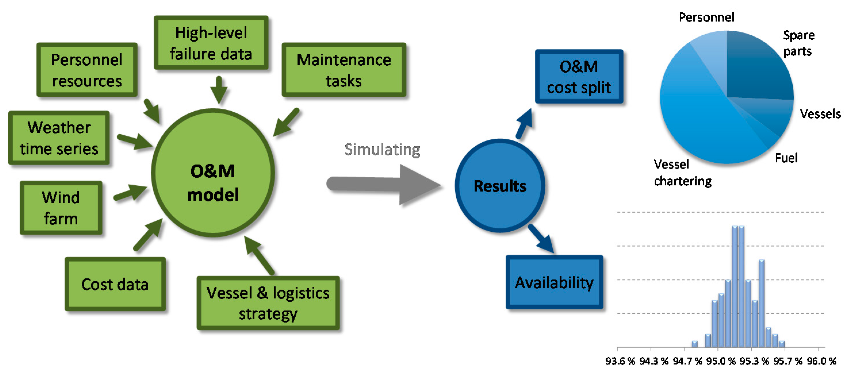
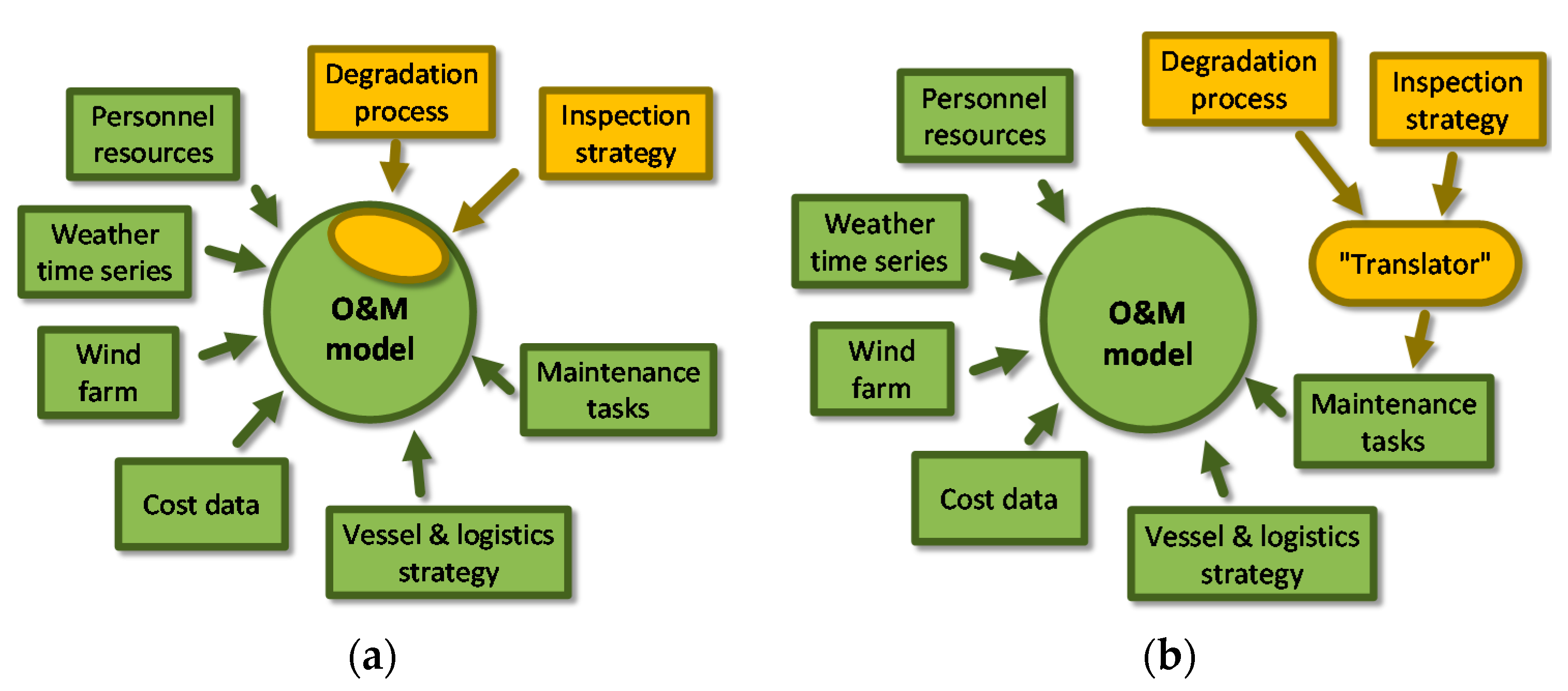
Several input parameters can be changed in order to assess their impact on performance parameters. Typical input and output parameters used in the NOWIcob model are illustrated in Figure 2. Offshore maintenance operations are highly weather-dependent, and weather conditions and uncertainty are thus accounted for in the model by means of a multi-parameter Markov chain weather model [7] that generates new and synthetic, but representative, weather time series for each Monte Carlo iteration (simulation run).
Maintenance tasks can be assigned to individual wind turbine components or can be assigned at a more aggregated level to the turbine as a whole. The three types of maintenance tasks modelled by NOWIcob are:
- (1)
- Pre-determined PM tasks, defined by a fixed maintenance interval.
- (2)
- CM tasks, each associated with a failure category.
- (3)
- CBM tasks, described in more detail below.
In the following, the modelling of a category of maintenance tasks in NOWIcob is referred to as a module, in which each module has certain input parameters that are used to describe a particular category. The CM module is based on a failure model in which the time to the next failure of a given failure category on a given turbine is drawn from an exponential probability density function . Here, is the underlying failure rate. The corresponding CM task is initiated after failure occurs.
The CBM module in NOWIcob is based on the following methodology: For each failure category associated with a CM task, a CBM task can also be defined in cases where condition monitoring or inspections can be used to detect degradation and an incipient failure. For a CBM task, the overall probability that an incipient failure is detected and a warning given (pdet) must be specified as input to the model, together with the pre-warning time (Tdet) and the underlying failure rate ().
Note that pdet is the overall probability of detection that applies to a certain inspection strategy and not the probability of detection (POD) of a flaw/crack of a given size by applying a given inspection method. See [39], among others, for further discussion of POD. Assuming that an inspection strategy is applied in situations where a certain inspection method (with corresponding POD) is regularly performed (e.g., once a year) and where maintenance tasks are initiated depending on the degradation of the component and inspection results, then pdet is the probability of detecting, with the given inspection strategy, an incipient failure before failure actually occurs. Consequently, 1-pdet is the probability of not detecting the incipient failure. pdet and 1-pdet thus describe the probability of occurrence of the detection and non-detection events, respectively, where detection results in a preventive maintenance task and non-detection in a corrective maintenance task.
On detection of an incipient failure, a warning is given that initiates the planning and execution of a CBM task. The pre-warning time Tdet is the number of days between the time of detection/warning and the time of potential failure. The time of potential failure is the time when failure would have occurred if the warning had not been given. Tdet can be specified as input to the model either in the form of a deterministic value or as a probability distribution in which case it is treated as a stochastic variable in the simulation. This simplified representation of CBM by the two parameters pdet and Tdet can be used to represent both continuous condition monitoring (i.e., condition monitoring systems) and inspections.
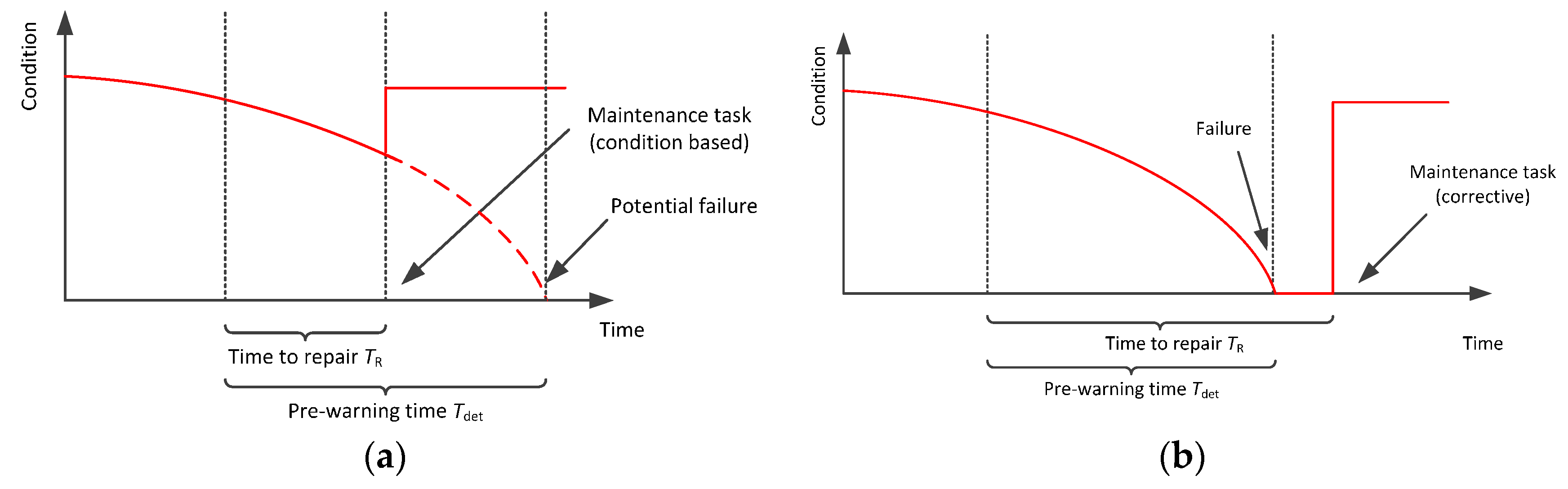
Figure 3 illustrates two possible outcomes of scenarios in which a potential failure is detected. The figure also illustrates the concept of the pre-warning time Tdet. Although an underlying degradation curve is indicated in the figure, it should be noted that degradation is not modelled explicitly in the CBM module. The time to repair (TR), also shown in the figure, is the time from the issue of the warning to completion of the maintenance task. The time to repair depends on the active maintenance time for the task in question plus logistic delays, including weather delays. The active maintenance time is defined as a model input parameter, whereas logistic delays are calculated during the simulation of each maintenance task.
If maintenance can be performed during the pre-warning time, i.e., TR < Tdet, then a CBM task is performed (see Figure 3a). On the other hand, if TR > Tdet, a CM task for the corresponding failure category is performed (see Figure 3b). It is also possible to model alternative responses to an early warning of a potential failure, such as shutting down the turbine when a pre-warning is given. The CBM task can be specified to require, for example, less expensive spare parts, shorter active repair times or shorter logistic delays than those for the CM task.
Different maintenance and inspection strategies will impact on pdet and Tdet. For example, more frequent inspections and conservative maintenance thresholds will result in increased pdet and Tdet values and, as a consequence, fewer failures and a reduced need for CM. However, the number of preventive maintenance tasks will increase. The relation between the maintenance strategy and quantities such as pdet and Tdet can be modelled using a degradation and maintenance model. The following section shows how such relations can be utilized to integrate degradation models and offshore wind farm O&M models.
3.2. Integration of the Degradation Process
As stated in the Introduction, this paper focuses on two integration alternatives referred to as full and loose integration. Full integration involves extension of the offshore wind O&M simulation model with the aim of modelling the degradation process inside the simulation model. Some of the disadvantages and challenges of this approach, such as increased computational time and the trade-off between detailed degradation modelling and the simplicity of input data representation, have already been referred to in the Introduction. Even though all types of degradation model could be applied using this approach, they must be implemented in the simulation model, and corresponding changes to the simulation model's user interface must be performed. Thus, integration alternatives should be evaluated with the aim of simplifying integration.
Loose integration is an alternative approach in which the simulation of degradation and the maintenance strategy is performed outside the wind farm O&M model using a so-called “translator”. The translator is a separate and relatively simple Monte Carlo simulator that can estimate more general (high-level) parameters such as pdet, Tdet and rates of inspection, maintenance and failure. Estimations are based on parameters describing the degradation process and maintenance strategy, such as Markov process transition rates, maintenance threshold and condition after maintenance. The translator thus “translates” the input of the degradation and maintenance model into input that can be applied by the maintenance modules that are already implemented in existing O&M models, such as NOWIcob’s module for CBM tasks (see Section 3.1).
Figure 4 illustrates how the two integration alternatives can be applied in connection with an O&M model such as NOWIcob. Segments colored yellow in the figure represent new model parts that are required for degradation process integration. Whereas full integration requires changes within the O&M model, loose integration keeps the O&M model untouched, because an existing NOWIcob maintenance module is used to link the degradation and maintenance model to the O&M model.
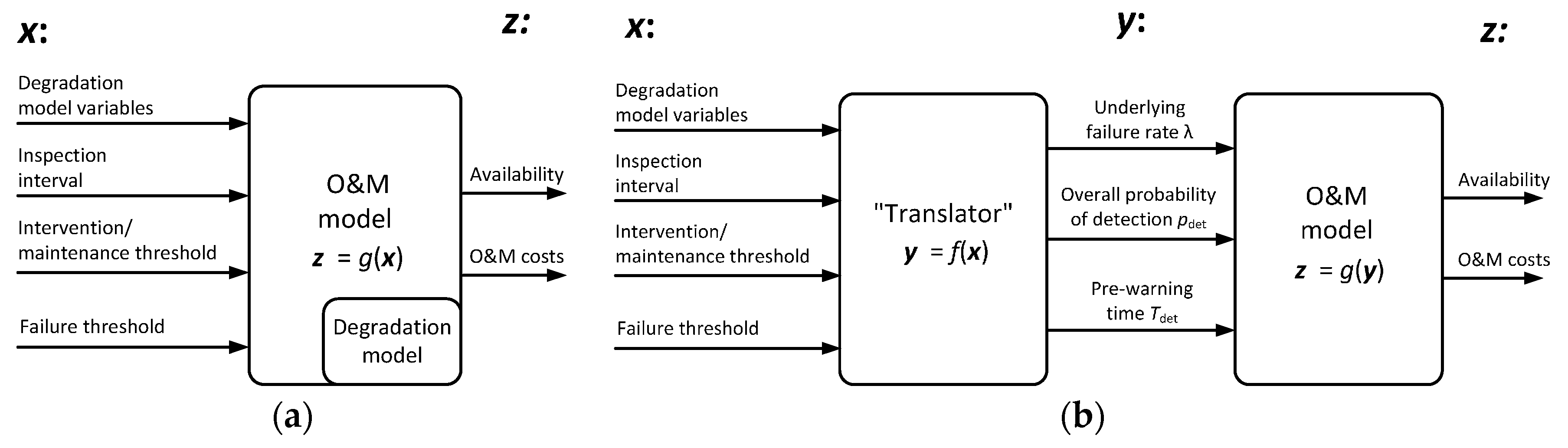
The two approaches used to integrate degradation processes in O&M models are illustrated in more detail in Figure 5. The parameters of the degradation and maintenance model, i.e., the variables that describe a degradation process and associated inspection strategy, are denoted by x. Figure 5a shows how x represents input parameters to the O&M model in the case where the degradation process is fully integrated. In contrast, in the loose integration approach, the O&M model input parameters are represented by the high-level input parameters y from the existing O&M model maintenance modules (Figure 5b). In this example, the CBM module input parameters are y = [pdet, Tdet, λ]. In mathematical terms, the translator used for loose integration of a certain type of degradation process and inspection strategy represents a function f: x → y. Furthermore, the O&M model represents a function g that calculates wind farm performance parameters z such as availability and O&M costs. These O&M model results can be expressed in the form zfull = gfull(x) for a fully-integrated degradation model and as zloose = gloose(y) = gloose(f(x)) for a loosely-integrated model. The simplified loose integration approach that decouples the degradation process from the O&M simulation can be viewed as an approximation of the full integration. The accuracy of this approximation can be assessed by comparing the values of zfull and zloose, i.e., by comparing the results from the O&M model for the two integration approaches.
The advantage of using the loose integration approach is that the translator represents a relatively simple and easily manageable model. In this way, different translators could easily be established for different types of degradation models and maintenance strategies without requiring changes in the code of comprehensive and sophisticated O&M simulation models. However, the disadvantage of loose integration is that it is likely to give less accurate results. Since full integration captures more of the real-world effects that may be crucial to accurate modelling, it represents the real world in a more complete and more realistic way than the simplified loose integration approach. This is illustrated in Table 1, which compares the full and loose integration approaches in terms of which effects are explicitly captured. Thus, the results of the full integration approach are regarded as a benchmark against which loose integration results can be compared. However, it is not always clear in advance which effects are most important for inclusion in the model, and this underlines the importance of analyzing the impact of different modelling assumptions.
A cross, X, against an effect in the table means that the effect is fully captured by the integration approach in question. A dash, -, means that the effect is not captured at all. A cross in parentheses, (X), means that the effect is only approximately captured because the simplified integration approach based on high-level input parameters estimated by the translator for the maintenance modules in the O&M model will lead to discrepancies.
4. Case Study
In order to compare the two alternative integration approaches, a Markov model for wind turbine blade degradation has been used as a case study. Blade degradation is based on the degradation model presented in [12], which presents a Markov chain consisting of seven states with state definitions and monthly transition probabilities as shown in Table 2. The Markov chain was transferred to a Markov process in which the transition time between the different states is exponentially distributed. The approximation λi = pi/(30 × 24) is used as the hourly transition rate, where the monthly transition probability from state i to state i + 1 is pi.
A simple annual inspection strategy is assumed, as illustrated in Figure 1, and the first inspection is scheduled for one year after commissioning of the wind farm. No maintenance actions will be performed if the blade condition is in States 0, 1, 2 or 3, and the next inspection is scheduled after one year. CBM will be initiated after an inspection if the blade is classified in States 4 or 5 (“serious damage” or “critical damage”). However, if the blade passes through degradation States 4 and 5 and reaches State 6 (“failure”) before this is detected by an inspection, a CM task must be initiated. After a CBM or a CM task has been carried out, the next inspection is scheduled after one year. The model assumes that inspections are perfect, i.e., the real deterioration states are detected without error [17].
For the loose integration approach, a translator was developed that simulates the degradation process and associated inspection strategy by means of a large number of Monte Carlo iterations. The proportion of iterations in which CBM is initiated before potential failure occurs is used to represent pdet. The mean time from the initiation of CBM to potential failure for these iterations is used to represent Tdet. (The impact of a more sophisticated approach, treating Tdet as a stochastic variable in NOWIcob, is briefly considered in the Supplementary Materials S2). It should be noted that CBM activities themselves and associated logistics are not modelled in the translator, but in the O&M model. The underlying failure rate associated with the degradation process (assuming no inspections) is calculated using the formula . The interaction between degradation and the associated inspection strategy is not explicitly represented in the NOWIcob model for loose integration. However, predetermined PM tasks with a fixed maintenance interval of one year are included in the simulations.
For the full integration approach, inspections, maintenance tasks and associated logistics are simulated inside the NOWIcob model. In this situation, inspections involve a crew transfer vessel transferring technicians to the wind turbine, if weather allows. The CBM task is assumed to be a relatively minor repair operation involving a crew transfer vessel. CM in this case involves a major blade replacement operation requiring a jack-up vessel. A fix-on-failure jack-up vessel charter strategy is assumed [40], with a mobilization time of 30 days from the date of vessel charter to the date of its availability to perform the maintenance task.
4.1. Wind Farm Scenario
The wind farm scenario assumed for the case study is based on a reference wind farm defined within the LEANWIND (Logistic Efficiencies And Naval architecture for Wind Installations with Novel Developments; EU FP7) project, consisting of 125 turbines, each with a power rating of 8 MW, located 30 km offshore from the O&M base. This reference wind farm is described in more detail in [40], and full specifications of the input data are found in the Supplementary Materials (S1).
The site of the reference wind farm corresponds to the location of West Gabbard in the U.K. North Sea. Since offshore wind farm O&M is known to be sensitive to on-site weather conditions and because conditions at the base case site are known to be relatively benign, two additional weather datasets are considered in the model: (1) data from the FINO (Forschungsplattformen in Nord- und Ostsee) 1 offshore research platform in the German North Sea [41], referred to as “medium weather”; and (2) data from the Heimdal natural gas field in the Norwegian North Sea [42], referred to as “harsh weather”. The FINO 1 and Heimdal weather datasets can be found in Supplementary Materials (S3) and (S4), respectively. Synthetic 25-year weather time series were generated based on the three weather datasets. This enables the case study to be carried out with a 25-year simulation period for all weather datasets, capturing variability in weather conditions that is representative for each of the sites.
4.2. Results Considering Single Component (Blades)
For the loose integration approach, the degradation process and inspection strategy described above were first simulated in the translator, independently of NOWIcob. For the given degradation process and annual inspection strategy, the overall probability of detection pdet simulated by the translator was 81.6%, and the pre-warning time Tdet 522 days. In order to consider an input data representation for this approach that is as simple as possible, the distribution of pre-warning time produced by the translator was not used in the O&M model for the results below (see, however, Supplementary Materials S2). In the absence of any inspections, the transition probabilities in Table 2 correspond to an underlying failure rate of λ = 0.2326 failures per turbine per year. The aforementioned values for pdet, Tdet and λ were used as input to the CBM module in NOWIcob for loose integration. For both loose integration and full integration, the 125-turbine wind farm scenario was simulated over 25 years using 1000 Monte Carlo iterations. The results of the simulations are given by the mean of all of the iterations, with an uncertainty estimate given by the standard error of the mean.
The ratio of simulated CBM tasks to the sum of simulated CM and CBM tasks can be compared with the pdet value calculated by the translator. For full integration, this ratio was found to be 81.4% for the base case, which is slightly lower than the value of 81.6% calculated by the translator. The main reason for this is that, in contrast to the translator, NOWIcob also takes account of the actual time to repair in the simulations, as illustrated in Figure 3. For loose integration, the 81.6% value calculated by the translator was used as input to NOWIcob, and the ratio of condition-based tasks calculated by NOWIcob was found to be 82.3%, i.e., slightly higher than pdet. The reasons for these differences will be explored further in Section 5.
Figure 6 shows results for average time-based wind turbine availability for the three weather datasets that were considered in both the full and loose integration approach. The uncertainty estimate for each data point is indicated by error bars. In both cases, wind turbine availability was reduced as weather conditions become harsher. Availability using the full integration approach is approximately between 0.02% and 0.03% lower than for loose integration. Although this difference is consistent and significant (the half-widths of the error bars are in the range 0.001–0.003%), the relative difference is only about 3% in terms of corresponding turbine downtime. Note that availability values in Figure 6 above 99% are higher than typical values for offshore wind farms because the case study only considers failures of a single component (blades). Results for energy-based availability were found to follow a very similar trend as time-based availability (see Supplementary Materials S2), but with somewhat larger differences that increased somewhat more for harsher weather conditions.
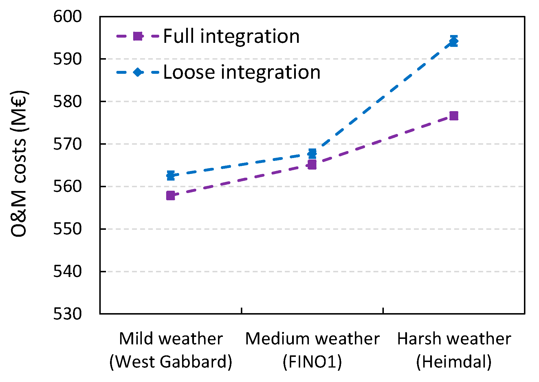
Figure 7 shows results for O&M costs, which include costs for vessel charter, fuel and spare parts for the full 25-year simulation period. The general trend indicates that O&M costs increase as weather conditions become harsher and that cost estimates for full integration are consistently lower than those for loose integration. The reason for this was found to be that fewer CM tasks are completed per jack-up vessel charter in simulations using the loose integration approach, which causes higher costs per CM task. The relative differences in O&M costs are in the range 0.5–0.9% for mild and medium weather conditions, but are significantly higher (3%) for harsh conditions. Relative uncertainties in the O&M cost estimates are in the range 0.14–0.18%.
4.3. Results Considering Multiple Components
The simulations presented in Figure 6 and Figure 7 above only considered failures of a single component (blades). The reason for this was to isolate the effect of blade degradation in the comparison of full and loose integration approaches. However, as an additional test, the case study is extended to consider a more complete failure dataset including failure categories involving all wind turbine components. This approach permits a comparison of the effect of blade degradation and failures with those for all other components. In other words, the results will indicate the relative importance of detailed blade degradation modelling. The dataset for multiple failure categories and failures for all components is the same as that presented and used in reference [40]. Note that these data include failure rates and not degradation model data. This has made it necessary to model additional failure categories using a failure rate model (using the CM module in NOWIcob) for both full and loose integration. Since the inclusion of all failure categories makes the simulation much more computationally demanding, the results are based on 500 Monte Carlo iterations. Furthermore, only one of the weather dataset (West Gabbard) was considered during this test.
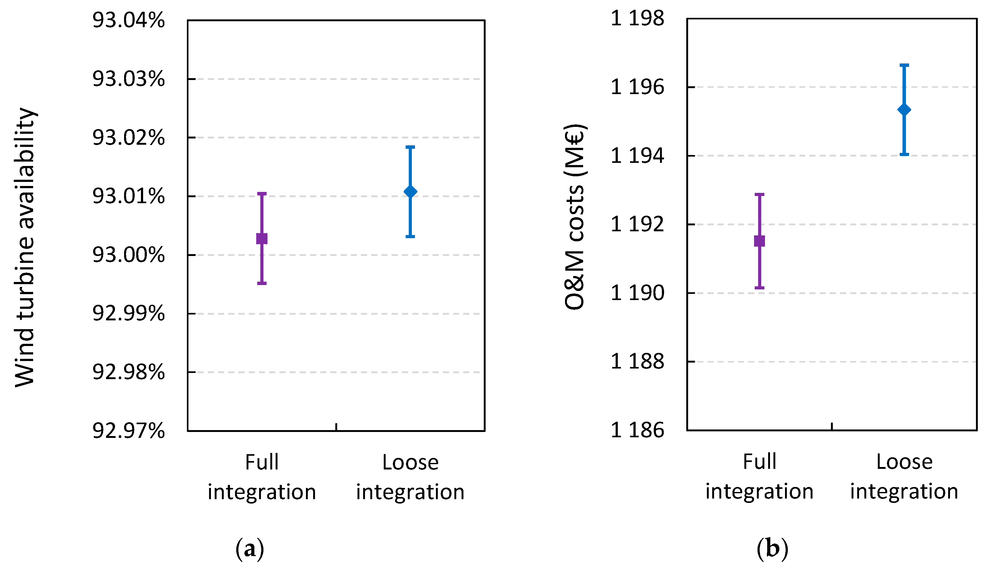
As shown in Figure 8, the inclusion of more failure categories causes wind turbine availability to decrease and O&M costs to increase in comparison with the results presented above. The inclusion also introduces greater stochasticity to the simulation, so that statistical variability and, hence, also statistical uncertainty increase for both performance parameters. There are very small differences between the values for full and loose integration for both performance parameters, compared to their uncertainty estimates. In the case of wind turbine availability, the difference between the two values is 0.008% and the uncertainty between 0.007% and 0.008%. However, if variance-reduction due to common random numbers is also considered in the estimate of the difference, the following inferences can be made (see Supplementary Materials S2 for details): (1) the availability value in the case of loose integration is most likely higher than for full integration; and (2) the difference is most likely smaller than for the case in which only blade failures were considered. In terms of O&M costs, the relative difference is 0.32% and relative uncertainties about 0.11%. For both availability and O&M costs, the relative differences between the results of full and loose integration approaches for blade degradation are smaller when multiple failure categories are included than when only blade failures are considered.
5. Discussion
The results from a comparison of full and loose integration approaches show that, for the case study, the differences between the aggregated result parameters for wind turbine availability and O&M costs are relatively small. More precisely, differences in downtime and O&M costs represent only very small percentages of total downtime and costs, respectively. Even though the loose integration approach fails to capture the effect of weather delays that prevent the detection of potential failures, results from loose integration are still similar to those from the full integration approach, even when weather conditions are harsher (we note here that differences may become more noticeable under very harsh weather conditions). Results from the two approaches are also similar when multiple failure categories are included in the simulations, and although statistical uncertainty increases, the relative differences decrease. Statistical uncertainty could be reduced further by increasing the number of Monte Carlo iterations, but in terms of providing an estimate of economic viability for an offshore wind farm project, we consider the precision to be adequate. Thus, we conclude that accuracy of the loose integration approach can be regarded as adequate in the context of this O&M model application when compared to the full integration approach.
Whether the accuracy of the loose integration approach is adequate for applications other than that presented here will depend on the decision problem in question and the relevant output parameters. Loose integration is likely to be adequate for decision problems related to maintenance and logistics that are not directly related to degradation of a specific component and its associated inspection strategy. For instance, there is little need to employ the full integration approach for an O&M model used to select the optimal vessel fleet for transferring technicians to wind turbines in order to carry out O&M.
On the other hand, if the decision is directly related to a problem such as determining the inspection strategy for blades, one may have to consider a full integration approach to the degradation model in order to achieve the required accuracy. For instance, if the intention is to co-optimize the timing of inspections and jack-up vessel campaign periods, one strategy may be to pre-charter a jack-up vessel for the month following the blade inspection campaign in case it transpires that a blade needs replacement. However, an analysis of this case will require explicit modelling of the inspection strategy. Additional results illustrating this interplay between jack-up vessel charter strategy and the inspection strategy can be found in the Supplementary Materials (S2). Furthermore, inspections and maintenance tasks generally do not occur at the same times throughout the year in the simulations of the O&M model for the two integration approaches. If application of the O&M model requires the study of a more detailed set of output parameters, such as the development of wind farm availability over time, one may also have to consider a full integration approach (cf. Supplementary Materials S2). This is discussed further below.
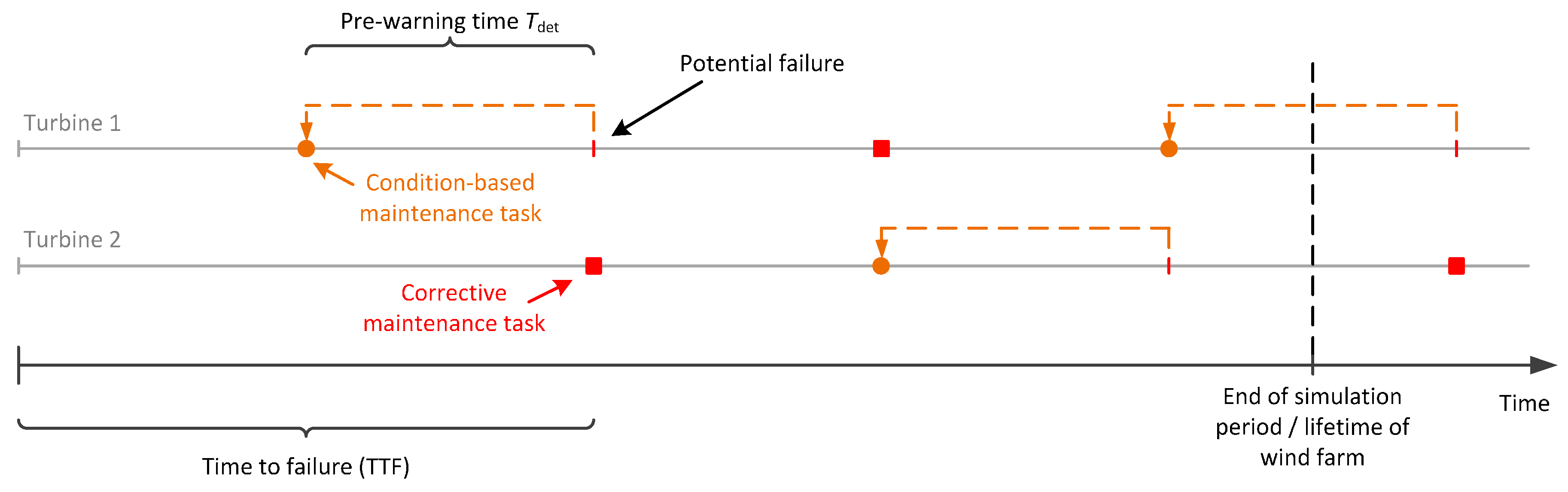
In the case of applying the loose integration approach to degradation modelling using NOWIcob’s CBM module as described in Section 3.1, the actual ratio of CBM tasks was found to be greater than the pdet value calculated by the translator. This effect is explained in Figure 9, which assumes a highly simplified case for the purposes of illustration: two turbines have one failure mode each and for which a potential failure can be detected with a probability pdet = 50%. It is also assumed that Tdet is equal to half of the mean time to failure (Tdet = 0.5 × MTTF) and that the time to repair is neglected (TTR = 0). Moreover, in Figure 9, the failures are plotted as occurring deterministically, with every second incipient failure being detected for each of the turbines. Although all of these assumptions are somewhat extreme, they do not influence the overall conclusion regarding the mechanisms at work.
As is seen in Figure 9, pre-warning time causes a “shift” of the CBM tasks to earlier points during the lifetime of the wind farm compared with a scenario in which the failure had not been detected. Nevertheless, in the long run, the ratio of CBM tasks remains the same at 50%. However, because simulations are carried out over a finite period (because the lifetime of the wind farm also is finite), the actual ratio of CBM tasks simulated will not necessarily be 50%. In the example shown in Figure 9, the number of CBM tasks exceeds CM tasks by one. This additional CBM task corresponds to a potential failure occurring after the lifetime of the wind farm. This effect explains why the ratio of CBM tasks resulting from the loose integration approach is slightly higher than the value of pdet provided by the translator.
A similar effect, whereby CBM tasks are “shifted backwards in time” relative to corrective tasks, is also observed for simulations using the full integration approach. However, here, the effect is less prominent than for loose integration. One reason for this is that the first opportunity for a CBM task to occur is after the first inspection. In the loose integration approach, on the other hand, a CBM task can be “shifted” to occur at earlier points in time. This effect is partly counterbalanced in full integration simulations by logistic delays that prevent inspections from detecting potential failures early enough; an effect that is not modelled in the calculation of pdet in the translator. The interplay of these different effects in the O&M model are subtle, but together they result in the actual ratio of condition-based tasks being slightly higher than the pdet value for loose integration and slightly lower than pdet for full integration, according to this study. This in turn leads to average wind turbine availability being slightly higher as a result of the loose integration approach than for full integration.
One may ask whether it is realistic, in the case of a potential failure, for the model to initiate a CBM task after the end of the lifetime of the wind farm (see Figure 9). However, in reality, when detecting a degraded state, the wind farm operator would not know whether the potential failure occurs before or after the end of the lifetime of the wind farm. Such end-of-life considerations represent an interesting aspect of overall maintenance strategy optimization, but are outside the scope of this study.
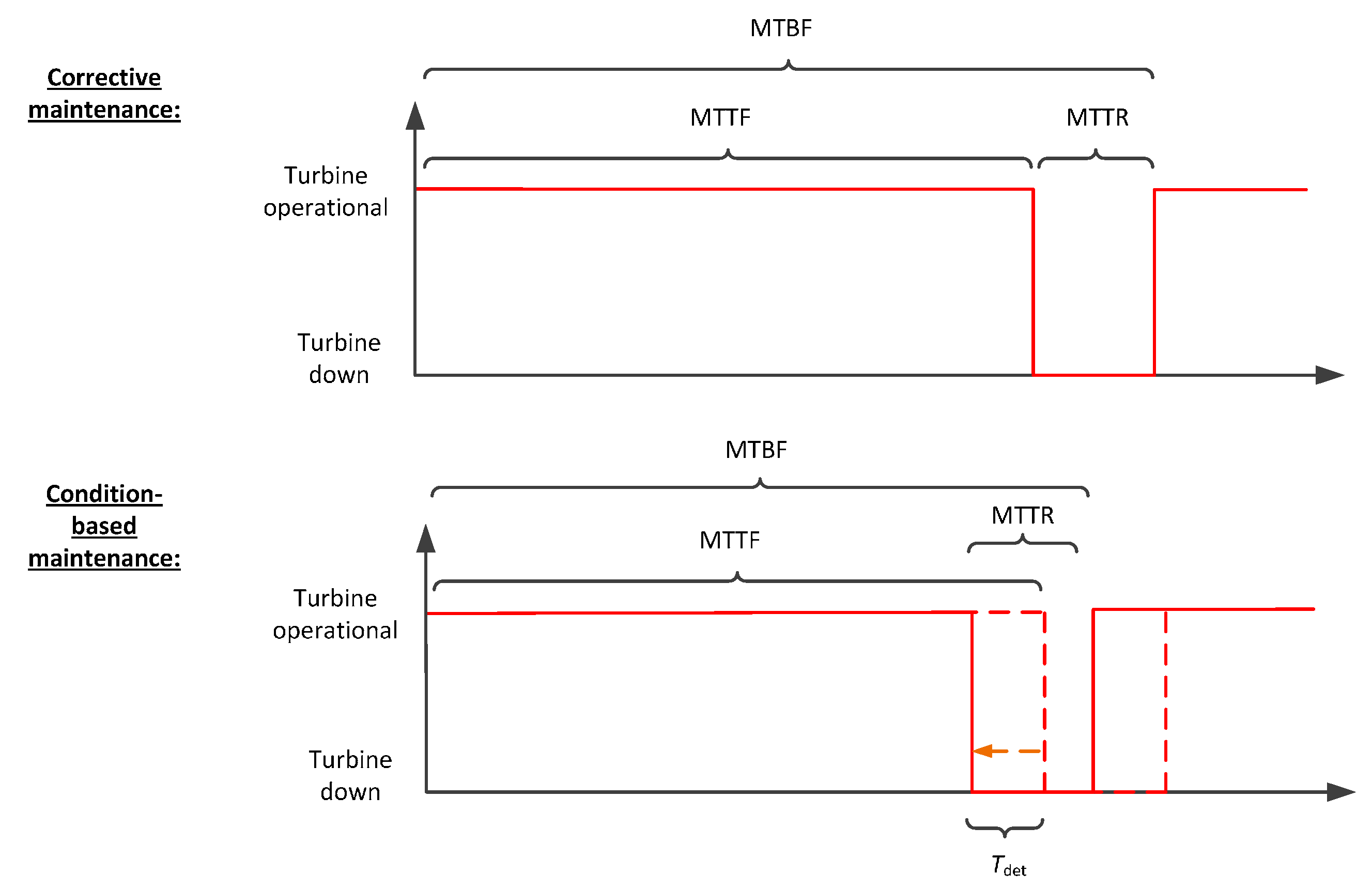
This investigation into the basic mechanisms of CBM also illustrates another effect. A CBM strategy may contribute towards increasing the number of maintenance tasks relative to a CM strategy. This proves to be the case not only in reality, but also following modelling using both the full and loose integration approaches. This effect is illustrated in simplified form in Figure 10. The actual rate of occurrence of CM tasks is given by 1/MTBF, where MTBF is an abbreviation for “mean time between failures”. The upper part of Figure 10 shows that MTBF = MTTF + MTTR. The lower part of the figure shows how MTBF changes for CBM tasks. The notation MTBF is used here, as well, but here relates to the mean time between maintenance tasks rather than failures. For CBM, MTBF = MTTF − Tdet + MTTR < MTTF + MTTR, which means that the rate of occurrence of maintenance tasks is higher than for CM.
In the case study, Tdet was relatively large compared to MTTF, and it was assumed for both the full and loose integration approaches that CBM was initiated as soon as an incipient failure was detected. However, in reality, this might not be a cost-effective maintenance strategy. Depending on the relative costs of a condition-based and a CM task, a greater number of maintenance tasks during the lifetime of the turbine might result in higher O&M costs. Furthermore, depending on the relative mean time to repair for CM and CBM, wind turbine availability may also be reduced as a result of a CBM strategy.
The decision problem of finding the optimal schedule for a CBM task given (imperfect) information about component condition and the degradation process provides an interesting direction for future research. However, since this paper focuses on strategic decision support, no sophisticated modelling of how an operator would solve this operational decision problem is attempted here. Nevertheless, an option has been implemented in the CBM module of NOWIcob that allows the user to specify how long after detection the CBM task will be initiated.
The time to repair is not given explicit consideration in the translator utilized for the loose integration approach. In order to obtain a more realistic pdet value, and thus improve the accuracy of the loose integration approach, one could also consider how it might be possible to represent repair of the component in the translator. However, modelling of the time to repair and its dependence on weather and logistics, etc., is precisely what the simulations in the full O&M model are intended to perform. Any increase in modelling sophistication in the translator would at some point defeat the purpose of loose integration, which is to simplify the approach compared to full integration.
Although the case study described in this paper was carried out using a particular O&M model (NOWIcob), the methodology for loose and full integration of degradation models is universal and not restricted to a particular tool. In broad terms, the majority of O&M tools are based on the same discrete-event simulation approach [1,43], and for this reason, the methodology for representing CBM and component degradation using a loose integration approach should be equally applicable for other O&M tools.
6. Conclusions
The full and loose integration approaches to degradation modelling each have their advantages. Given detailed and accurate input data, full integration provides somewhat more accurate results. This is at least the case if we consider detailed output parameters such as the time dependence of wind turbine availability, but less so when considering aggregated output parameters such as average wind turbine availability. Furthermore, full integration implies a more detailed representation of the inspection and maintenance strategy and, thus, allows for better decision support if the decision problem in question is to optimize these strategies.
On the other hand, loose integration is easier to carry out because it does not require the implementation and integration of each specific degradation model together with corresponding inspection strategies in the O&M model. Instead, one can use a generic module for condition-based maintenance in the O&M model that has simpler input data representation based on the high-level failure data format conventionally used in O&M models. This approach provides flexibility with respect to data availability. If necessary, and when knowledge of the degradation process is available, degradation can be represented in this module by implementing a translator that generates the necessary input parameters. If knowledge is lacking, input parameters such as pdet and Tdet can either be estimated based on existing failure and maintenance statistics or available data can be supplemented by input values judged by experts.
Supplementary Materials
The following materials are available online at www.mdpi.com/1996-1944/10/7/925/s1: Note S1: Input data used for “Integration of Degradation Processes in a Strategic Offshore Wind Farm O&M Simulation Model”; Note S2: Supplementary results for “Integration of Degradation Processes in a Strategic Offshore Wind Farm O&M Simulation Model”; Table S3: FINO1 weather data; Table S4: Heimdal weather data.
Acknowledgments
This project has received funding from the European Union’s 7th Framework Programme for Research and Technological Development under Grant Agreement No. 614020 (LEANWIND) and was co-funded by the Research Council of Norway and industry partners through the Norwegian Research Centre for Offshore Wind Technology (NOWITECH). The authors wish to thank partners in the LEANWIND project for fruitful discussions on the concept underlying this work and the anonymous reviewers for their thorough feedback that has helped in improving the quality of this paper. The authors also wish to thank BMU (Bundesministerium fuer Umwelt, Federal Ministry for the Environment, Nature Conservation and Nuclear Safety) and PTJ (Projekttraeger Juelich, project executing organization) for providing data from the FINO project.
Author Contributions
T.M. Welte, I.B. Sperstad and M.L. Kolstad conceived of and developed the main idea for this work. All of the authors contributed to the definition of the case study. E.H. Sørum, I.B. Sperstad and M.L. Kolstad implemented the various integration approaches using the existing NOWIcob model, developed and coded the translator tool, and they performed simulations and calculations using the tools. All authors jointly analyzed and discussed the results. T.M. Welte, I.B. Sperstad and M.L. Kolstad wrote the paper, which was subsequently thoroughly reviewed by all of the authors.
Conflicts of Interest
The authors declare no conflict of interest.
References
- Welte, T.M.; Sperstad, I.B.; Espeland Halvorsen-Weare, E.; Netland, Ø.; Nonås, L.M.; Stålhane, M. O&M modelling. In Offshore Wind Energy Technology; Anaya-Lara, O., Tande, J.O., Uhlen, K., Merz, K., Eds.; Wiley: Chichester, West Sussex, UK, 2017; in press. [Google Scholar]
- Hofmann, M. A review of decision support models for offshore wind farms with an emphasis on operation and maintenance strategies. Wind Eng. 2011, 35, 1–16. [Google Scholar] [CrossRef]
- Shafiee, M. Maintenance logistics organization for offshore wind energy: Current progress and future perspectives. Renew. Energy 2015, 77, 182–193. [Google Scholar] [CrossRef]
- Rademakers, L.W.M.M.; Braam, H.; Obdam, T.S.; van de Pieterman, R.P. Operation and Maintenance Cost Estimator (OMCE); Report No. ECN-E–09-037; Energy Research Centre of The Netherlands (ECN): Petten, The Netherlands, 2009. [Google Scholar]
- Douard, F.; Domecq, C.; Lair, W. A probabilistic approach to introduce risk measurement indicators to an offshore wind project evaluation—Improvement to an existing tool. Energy Procedia 2012, 24, 255–262. [Google Scholar] [CrossRef]
- Dalgic, Y.; Lazakis, I.; Dinwoodie, I.; McMillan, D.; Revie, M. Advanced logistics planning for offshore wind farm operation and maintenance activities. Ocean Eng. 2015, 101, 211–226. [Google Scholar] [CrossRef]
- Hofmann, M.; Sperstad, I.B. NOWIcob—A tool for reducing the maintenance costs of offshore wind farms. Energy Procedia 2013, 35, 177–186. [Google Scholar] [CrossRef]
- Faulstich, S.; Berkhout, V.; Mayer, J.; Siebenlist, D. Modelling the failure behaviour of wind turbines. J. Phys. Conf. Ser. 2016, 749, 012019. [Google Scholar] [CrossRef]
- Dewan, A. Logistic & Service Optimization for O&M of Offshore Wind Farms. Master’s Thesis, Delft University of Technology, Delft, The Netherlands, 2014. [Google Scholar]
- Nielsen, J.J.; Sørensen, J.D. On risk-based operation and maintenance of offshore wind turbine components. Reliab. Eng. Syst. Saf. 2011, 96, 218–229. [Google Scholar] [CrossRef]
- Florian, M.; Sørensen, J.D. Planning of operation & maintenance using risk and Reliability based methods. Energy Procedia 2015, 80, 357–364. [Google Scholar]
- Florian, M.; Sørensen, J.D. Case study for impact of D-String® on levelized cost of energy for offshore wind turbine blades. Int. J. Offshore Polar Eng. 2017, 27, 63–69. [Google Scholar] [CrossRef]
- International Electrotechnical Commission. 60050-192: International Electrotechnical Vocabulary—Part 192: Dependability; International Electrotechnical Commission (IEC): Geneva, Switzerland, 2015. [Google Scholar]
- Meeker, W.Q.; Escobar, L.A. Statistical Methods for Reliability Data; Wiley: New York, NY, USA, 1998. [Google Scholar]
- Welte, T.M.; Wang, K. Models for lifetime estimation: An overview with focus on applications to wind turbines. Adv. Manuf. 2014, 2, 79–87. [Google Scholar] [CrossRef]
- Ross, S.M. Stochastic Processes; Wiley: New York, NY, USA, 1996. [Google Scholar]
- Welte, T. Deterioration and Maintenance Models for Components in Hydropower Plants. Ph.D. Thesis, Norwegian University of Science and Technology, Trondheim, Norway, 2008. [Google Scholar]
- Kallen, M.J. Markov Processes for Maintenance Optimization of Civil Infrastructure in the Netherlands. Ph.D. Thesis, Delft University of Technology, Delft, The Netherlands, 2007. [Google Scholar]
- Nicolai, R.P.; Dekker, R.; van Noortwijk, J.M. A comparison of models for measurable deterioration: An application to coatings on steel structures. Reliab. Eng. Syst. Saf. 2007, 92, 1635–1650. [Google Scholar] [CrossRef]
- Van Noortwijk, J.M. A survey of the application of gamma processes in maintenance. Reliab. Eng. Syst. Saf. 2009, 94, 2–21. [Google Scholar] [CrossRef]
- Hameed, Z.; Vatn, J. State based models applied to offshore wind turbine maintenance and renewal. In Advances in Safety, Reliability and Risk Management, Proceedings of the European Safety and Reliability Conference (ESREL) 2011, Troyes, France, 18–22 September 2011; Berenguer, C., Grall, A., Soares, C.G., Eds.; CRC Press/Balkema: Leiden, The Netherlands, 2012; pp. 989–996. [Google Scholar]
- Besnard, F.; Bertling, L. An approach for condition-based maintenance optimization applied to wind turbine blades. IEEE Trans. Sustain. Energy 2010, 1, 77–83. [Google Scholar] [CrossRef]
- Byon, E.; Ding, Y. Season-dependent condition-based maintenance for a wind turbine using a partially observed Markov decision process. IEEE Trans. Power Syst. 2010, 25, 1823–1834. [Google Scholar] [CrossRef]
- Shafiee, M.; Finkelstein, M.; Bérenguer, C. An opportunistic condition-based maintenance policy for offshore wind turbine blades subjected to degradation and environmental shocks. Reliab. Eng. Syst. Saf. 2015, 142, 463–471. [Google Scholar] [CrossRef]
- Shafiee, M.; Finkelstein, M. An optimal age-based group maintenance policy for multi-unit degrading systems. Reliab. Eng. Syst. Saf. 2015, 134, 230–238. [Google Scholar] [CrossRef]
- Flory, J.A.; Kharoufeh, J.P.; Abdul-Malak, D.T. Optimal replacement of continuously degrading systems in partially observed environments. Nav. Res. Logist. 2015, 62, 395–415. [Google Scholar] [CrossRef]
- Ossai, C.I.; Boswell, B.; Davies, I.J. A Markovian approach for modelling the effects of maintenance on downtime and failure risk of wind turbine components. Renew. Energy 2016, 96, 775–783. [Google Scholar] [CrossRef]
- Shafiee, M.; Finkelstein, M. A proactive group maintenance policy for continuously monitored deteriorating systems: Application to offshore wind turbines. Proc. Inst. Mech. Eng. Part O J. Risk Reliab. 2015, 229, 373–384. [Google Scholar] [CrossRef]
- Dawid, R.; McMillan, D.; Revie, M. Review of Markov models for maintenance optimization in the context of offshore wind. In Proceedings of the Annual Conference of the Prognostics and Health Management Society 2015, San Diego, CA, USA, 19–24 October 2015; Daigle, M.J., Bregon, A., Eds.; pp. 269–279. [Google Scholar]
- Le, B.; Andrews, J. Modelling wind turbine degradation and maintenance. Wind Energy 2016, 19, 571–591. [Google Scholar] [CrossRef]
- Rausand, M.; Høyland, A. System Reliability Theory: Models, Statistical Methods, and Applications, 2nd ed.; John Wiley & Sons: Hoboken, NJ, USA, 2004. [Google Scholar]
- Welte, T.M. A theoretical study of the impact of different distribution classes in a Markov model. In Risk, Reliability and Societal Safety, Proceedings of the European Safety and Reliability Conference (ESREL) 2007, Stavanger, Norway, 25–27 June 2007; Aven, T., Vinnem, J.E., Eds.; CRC Press: Leiden, The Netherlands, 2007. [Google Scholar]
- Welte, T.M. A rule-based approach for establishing states in a Markov process applied to maintenance modelling. Proc. Inst. Mech. Eng. Part O J. Risk Reliab. 2008, 223, 1–12. [Google Scholar] [CrossRef]
- Neuts, M.F. Probability distributions of phase type. In Matrix-Geometric Solutions in Stochastic Models; The John Hopkins University Press: Baltimore, MD, USA, 1981; pp. 41–80. [Google Scholar]
- Asmussen, S.; Nerman, O.; Marita, O. Fitting phase-type distributions via the EM algorithm. Scand. J. Stat. 1996, 23, 419–441. [Google Scholar]
- Olsson, M. EM Estimation in Phase Type Models. Ph.D. Thesis, Chalmers Technical University, Gøteborg, Sweden, 1995. [Google Scholar]
- Olsson, M. The EMpht-Programme. User Guide for the EMpht-Programme. Available online: http://home.imf.au.dk/asmus/dl/EMusersguide.ps (accessed on 19 June 2017).
- Hofmann, M.; Sperstad, I.B.; Kolstad, M. Technical Documentation of the NOWIcob Tool (DB.1-2); Report No. TR A7374; SINTEF Energy Research: Trondheim, Norway, 2015. [Google Scholar]
- DNV GL AS. Probabilistic Methods for Planning of Inspection for Fatigue Cracks in Offshore Structures; DNVGL-RP-0001; DNV GL AS: Oslo, Norway, 2015. [Google Scholar]
- Sperstad, I.B.; McAuliffe, F.D.; Kolstad, M.; Sjømark, S. Investigating key decision problems to optimise the operation and maintenance strategy of offshore wind farms. Energy Procedia 2016, 94, 261–268. [Google Scholar] [CrossRef]
- Bundesamt für Seeschifffahrt und Hydrographie (BSH). FINO—Datenbank. Available online: http://fino.bsh.de/ (accessed on 1 December 2012).
- Norwegian Meteorological Institute. eKlima. Available online: http://www.eklima.no/ (accessed on 9 June 2013).
- Dinwoodie, I.; Endrerud, O.-E.V.; Hofmann, M.; Martin, R.; Sperstad, I.B. Reference cases for verification of operation and maintenance simulation models for offshore wind farms. Wind Eng. 2015, 39, 1–14. [Google Scholar] [CrossRef]
Figure 1.
Illustration of a degradation process modelled as a continuous-time Markov process: (a) degradation process, condition states and inspection strategy; (b) the Markov process and maintenance strategy.
Figure 1.
Illustration of a degradation process modelled as a continuous-time Markov process: (a) degradation process, condition states and inspection strategy; (b) the Markov process and maintenance strategy.
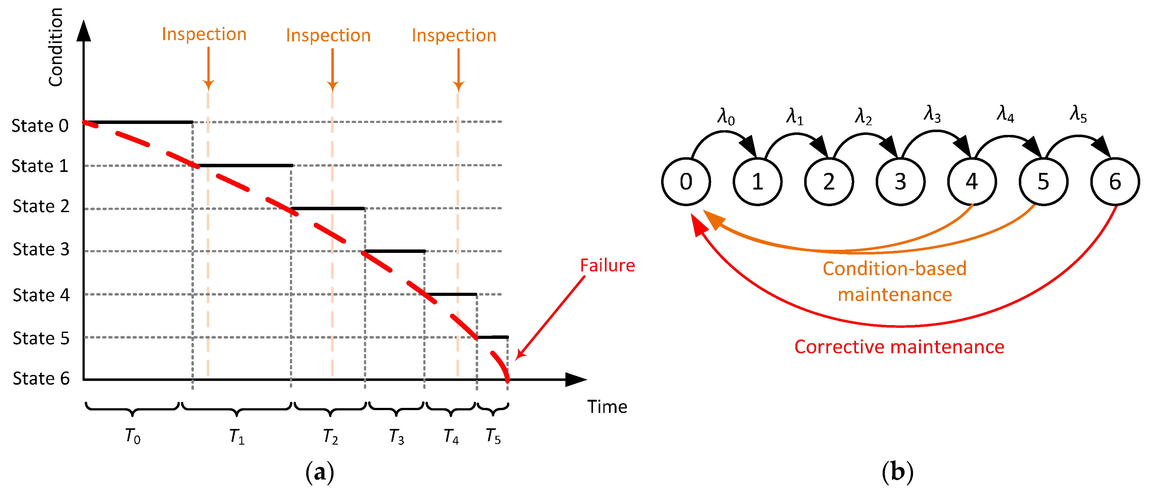
Figure 2.
Typical input and output parameters of NOWIcob.

Figure 3.
Possible outcomes of scenarios in which a potential failure is detected: (a) outcome for TR < Tdet, resulting in CBM; (b) outcome for TR > Tdet, resulting in CM.
Figure 3.
Possible outcomes of scenarios in which a potential failure is detected: (a) outcome for TR < Tdet, resulting in CBM; (b) outcome for TR > Tdet, resulting in CM.

Figure 4.
NOWIcob input parameters and a conceptual illustration of two alternative integration approaches: (a) full integration; (b) loose integration.
Figure 4.
NOWIcob input parameters and a conceptual illustration of two alternative integration approaches: (a) full integration; (b) loose integration.

Figure 5.
Illustration of the two integration approaches: (a) full integration; (b) loose integration.
Figure 5.
Illustration of the two integration approaches: (a) full integration; (b) loose integration.

Figure 6.
Results for average time-based wind turbine availability under different weather conditions.
Figure 6.
Results for average time-based wind turbine availability under different weather conditions.

Figure 7.
Results for O&M costs for different weather conditions.

Figure 8.
Results for a failure data set that includes all wind turbine components: (a) average time-based wind turbine availability; (b) O&M costs.
Figure 8.
Results for a failure data set that includes all wind turbine components: (a) average time-based wind turbine availability; (b) O&M costs.

Figure 9.
Illustration of the effect of pre-warning time on the time of CBM tasks.

Figure 10.
Illustration of the effect of CBM on the mean time between maintenance tasks.

Table 1.
Effects captured using full and loose integration of degradation processes. CBM, condition-based maintenance.
Table 1.
Effects captured using full and loose integration of degradation processes. CBM, condition-based maintenance.
| Effect | Full Integration | Loose Integration |
|---|---|---|
| Logistic delay (including weather delay) in the time to repair. | X | X |
| Logistic delays (including weather delays) that prevent detection of potential failure. | X | - |
| Dependence of inspection interval on component condition. | X | (X) |
| Distribution of inspections over wind farm lifetime. | X | - |
| Distribution of CBM tasks over wind farm lifetime. | X | - |
| Stochasticity of pre-warning time. | X | (X) |
| Costs and resource requirements for inspections. | X | X |
Table 2.
States of the degradation process and transition probabilities, based on [12].
Table 2.
States of the degradation process and transition probabilities, based on [12].
| State i | State Definition | Transition Probability pi (1/Month) |
|---|---|---|
| 0 | No damage | 0.05 |
| 1 | Cosmetic damage | 0.75 |
| 2 | Minor Damage, below tear and wear | 0.27 |
| 3 | Minor damage, above tear and wear | 0.13 |
| 4 | Serious damage | 0.06 |
| 5 | Critical damage | 0.344 |
| 6 | Failure | n/a |
© 2017 by the authors. Licensee MDPI, Basel, Switzerland. This article is an open access article distributed under the terms and conditions of the Creative Commons Attribution (CC BY) license (http://creativecommons.org/licenses/by/4.0/).
Share and Cite
MDPI and ACS Style
Welte, T.M.; Sperstad, I.B.; Sørum, E.H.; Kolstad, M.L. Integration of Degradation Processes in a Strategic Offshore Wind Farm O&M Simulation Model. Energies 2017, 10, 925. https://doi.org/10.3390/en10070925
AMA Style
Welte TM, Sperstad IB, Sørum EH, Kolstad ML. Integration of Degradation Processes in a Strategic Offshore Wind Farm O&M Simulation Model. Energies. 2017; 10(7):925. https://doi.org/10.3390/en10070925
Chicago/Turabian StyleWelte, Thomas Michael, Iver Bakken Sperstad, Espen Høegh Sørum, and Magne Lorentzen Kolstad. 2017. "Integration of Degradation Processes in a Strategic Offshore Wind Farm O&M Simulation Model" Energies 10, no. 7: 925. https://doi.org/10.3390/en10070925
Note that from the first issue of 2016, this journal uses article numbers instead of page numbers. See further details here.