Tracking Control with Zero Phase-Difference for Linear Switched Reluctance Machines Network
by
 , ,
, ,
Bo Zhang
1,2 ,
,
J.F. Pan
1 ,
,
Jianping Yuan
2,*,
Wufeng Rao
1,2,
Li Qiu
1,
Jianjun Luo
2 and
Honghua Dai
2 1
College of Mechatronics and Control Engineering, Shenzhen University, Shenzhen 518060, China;[email protected] (B.Z.); [email protected] (J.F.P.); [email protected] (W.R.); [email protected] (L.Q.)
2
Laboratory of Advanced Unmanned Systems Technology, Northwestern Polytechnical University,Shenzhen 518060, China; [email protected] (J.L.); [email protected] (H.D.)
*
Author to whom correspondence should be addressed.
Energies 2017, 10(7), 949; https://doi.org/10.3390/en10070949
Submission received: 26 April 2017
/
Revised: 16 June 2017
/
Accepted: 4 July 2017
/
Published: 8 July 2017
(This article belongs to the Special Issue Networked and Distributed Control Systems)
Abstract
:This paper discusses the control of the linear switched reluctance machines (LSRMs) network for the zero phase-difference tracking to a sinusoidal reference. The dynamics of each LSRM is derived by online system identification and modeled as a second-order linear system. Accordingly, based on the coupled harmonic oscillators synchronization manner, a distributed control strategy is proposed to synchronize each LSRM state to a virtual LSRM node representing the external sinusoidal reference for tracking it with zero phase-difference. Subsequently, a simulation scenario and an experimental platform with the identical parameter setup are designed to investigate the tracking performance of the LSRMs network constructed by the proposed distributed control strategy. Finally, the simulation and experimental results verify the effectiveness of the proposed LSRMs network controller, and also prove that the coupled harmonic oscillators synchronization method can improve the synchronization tracking performance and precision.
1. Introduction
Linear tracking control systems based on direct drive linear machines are vastly used in the manufacturing industry, such as parts assembly, printed circuit boarding (PCB) drilling and chip processing, etc. In addition, there are many tasks that require a cooperation of many linear machines to work harmonically. For example, in a multi-station PCB drilling machine, each linear machine acts as one working unit. The board being processed requires the linear machines to track the command position precisely and coordinates with each other to finish the whole drilling work. Therefore, each linear machine often demands the state information from other machines, so as to work cooperatively and synchronously. The overall motion control performance can be improved such as faster operation time, more efficiency and the annihilation of accumulated errors, etc., compared to a traditional sequenced working manner [1]. Furthermore, if multiple linear machines can be organized as a coordinated and distributed motion tracking network and each machine has the position controller, sensor and driver of its own, the ultimate global tracking control goal can be emerged by local communications among the independent linear machine nodes with local controllers, without the necessity of any global supervision or decision [2].
Among different types of linear machines, a linear switched reluctance motor (LSRM) has the advantages of a simple and robust mechanical structure, low cost, high reliability and free of frequent maintenance or adjustments [3]. Current motion tracking research on LSRMs mainly focuses on the control performance improvement for single machine based position control systems [4,5,6,7]. In [4], an adaptive position controller is inspected to compensate uncertain behaviors of a double-sided LSRM. A nonlinear proportional differential (PD) tracking controller based on the tracking differentiator is proposed for a real-time LSRM suspension system, to achieve a better dynamic position response [5]. A sliding mode position control technique is investigated in [6] and a passivity-based control algorithm is proposed for the LSRM position tracking system to overcome the inherent nonlinear characteristics and ameliorate system robustness against uncertainties and bounded disturbances [7]. From the latest development on the tracking control performance of LSRMs, the ratio of an absolute dynamic tracking error to full range of 5% can be achieved in single LSRM position control applications.
As mentioned above, by employing a multi-agent network formed by distributed control on the same product line, all LSRMs can be coordinated to work together harmonically. Up until now, the experiment and technique studies on the tracking control network based on LSRMs have gained much attention, and related research is increasing [8,9]. Current analysis of motion coordinated control of multi-agent networks mainly focuses on distributed control methods with multi-agent networks [10,11,12,13,14,15,16], which provides a guidance to the LSRMs network. Reference [10] primarily investigated the consensus for coordinated control of multi-agent networks, and established the connections between structural properties and the performance of networks. Cao et al. [11] elaborated the main results and the progress about coordinated control algorithms for multi-agent networks and summarized the future directions of the distributed coordination of multi-agent. At present, multi-agent network study has been classified into several major aspects, which include constrained or imperfect communication [12], delay or switching information linkage [13,14], agents with nonlinear dynamics [15], influence of noise [16], etc., Furthermore, the multi-agent networks bound by distributed control algorithms have been exploited in the regime of spacecraft cluster [17], robot coordination [18], and unmanned aerial vehicle formation [19].
It can be concluded from the above analysis that current theoretical work mainly concentrates on distributed control methods to achieve the network synchronization under some network topology constraint condition. The ultimate goal is to form a stable synchronized motion among the multiple agents within the network employing distributed and networked control algorithms. However, in most industry processes, multiple LSRMs composing a multi-agent network are not only required for motion synchronization but also to track some specific desired trajectory [20]. In practice, directly controlling every agent in a multi-agent network with a number of agents might be impossible or unnecessary. Therefore, pinning control is regarded as a desirable method [21]. Accordingly, the multi-agent network formed by the pinning control is defined as the leader-following network [2]. In a leader-following network, a reference can be accessed directly by minority agents named as leaders only, and then the rest of the agents named as followers are steered to implement the synchronized motion to the common reference by the effect of the distributed control. Wang et al. [22] elaborately reviewed advances in pinning control approaches, including the feasibility, stability and effectiveness of pinning control and pinning-based consensus and flocking control of mobile multi-agent networked systems. One of the challenges with a leader-following network is that the reference possesses different dynamic characteristics from all agents. Cao et al. [23] proposed a distributed consensus tracking algorithm for second-order dynamics guarantees global exponential tracking without acceleration measurements, and the dynamic reference was modeled as the virtual leader with time-varying velocity. Especially, in industrial processes, for implementing much of repetitive work, some periodic motion modes such as sinusoid always were as the desired motion. Wang et al. [24] proposed an internal model controller compensating the reference dynamics for output synchronization of more general heterogeneous multi-agents systems. Wieland et al. [25] proved that an internal model principle is necessary and sufficient for exponential synchronizability of the group to some common, non-trivial output trajectory, bounded by a polynomial function in time, and also note that the internal model components may give rise to the instability of the multi-agent network under the influence of parametric uncertainties.
In this paper, the mathematical model of each LSRM is derived by the online system identification, which is essentially modeled as a general second-order linear system. Second, inspired by coupled harmonic oscillators [26,27], a distributed control is designed to track a sinusoidal reference with zero phase-difference among each LSRM and the reference as virtual node, so as to improve the tracking performance of the LSRMs network. Last, simulation and experimental verification is provided to prove the effectiveness of the network controller design scheme.
The main contributions of this paper are threefold. First, for the convenience of the coordinated motion control, the reference signal is modeled as a virtual LSRM node that has the same dynamic characteristics as three motor nodes based on the proposed distributed tracking control strategy. Second, three motor nodes and the virtual node can be realized by the synchronization control by adopting the coupled harmonic oscillators method, so as to achieve for tracking the sinusoidal reference signal with zero phase-difference. Finally, the distributed tracking control performance for the LSRMs network is investigated by a simulation and experimental platform testing.
2. Model and Preliminaries
2.1. Mathematical Preliminaries
Notations: Let and indicate the n-dimensional Euclidean space and the set of real matrices, respectively. represents an N-dimension unit matrix. The Kronecker product of matrices and satisfies the following properties as:
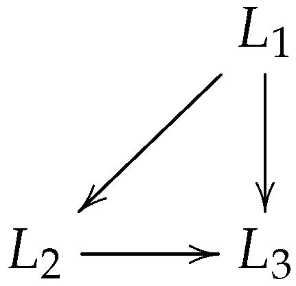
The interaction topology of the coordinated network building LSRMs network system is represented using a directed graph , as shown in Figure 1, which is characterized by an edge-linked node set . It denotes N local closed-loop LSRM systems termed as LSRM node , formed by each LSRM and its local controller individually. An edge set represents M communication linkages among all LSRM nodes, where an edge exists from LSRM node to if . If a set composed of LSRM nodes satisfies , it is named as the neighbor set associated with the LSRM node . A directed graph contains a directed spanning tree if there exists a node called root such that there is one or more than one directed path from this node to every other node, such as in Figure 1. A path from to in is formed by the subset . denote its adjacency matrix and Laplacian matrix of , respectively.
2.2. Model of Linear Switched Reluctance Machine Node
Any of the N three-phase LSRMs (indexed as i-th, ) can be described in the voltage equation as [4]:
where , and are terminal voltage, coil resistance and current, respectively. represents the flux-linkage of the k-th winding. Each LSRM can also be depicted as the second-order dynamics as follows:
where , , , and represent position, friction coefficient, mass, total and load force of the i-th LSRM, respectively. The second-order system as Equation (3) can be further represented in the discrete-time form as [5]:
where and are polynomials to be determined, z is the discrete-time operator, and denotes stochastic disturbances of the i-th LSRM.The polynomials and corresponding to the typical discrete-time form are depicted as:
The purpose of online system identification is to correctly estimate , , and that contain all dynamic information of each LSRM. For the n-th estimation, Equation (4) can also be considered as a typical least square form as follows:
where is the i-th LSRM state including the position and velocity at time step k, and:
where is the vector to be estimated, and is the matrix that include the input and output information of x and f. The parameters , described in Equation (7) can be estimated by the recursive least square method as [29]:
where P is the covariance matrix and R is the gain, K and I are, respectively, the gain matrix and an identity matrix with compatible dimensions, and represents the estimated value of through the identification process. is the forgetting factor that reflects the relationship between the converging rate and tracking ability and it falls into 0 and 1. For the LSRM, is chosen as for moderate converging ripples and a fast identification speed. For initial values, can be chosen as with as a constant value of 50. Stochastic errors can be represented as:
If the relative error from the present to the last step is comparatively a small positive value , it can be regarded that the present estimated value is correct. Then, the termination criterion can be represented as:
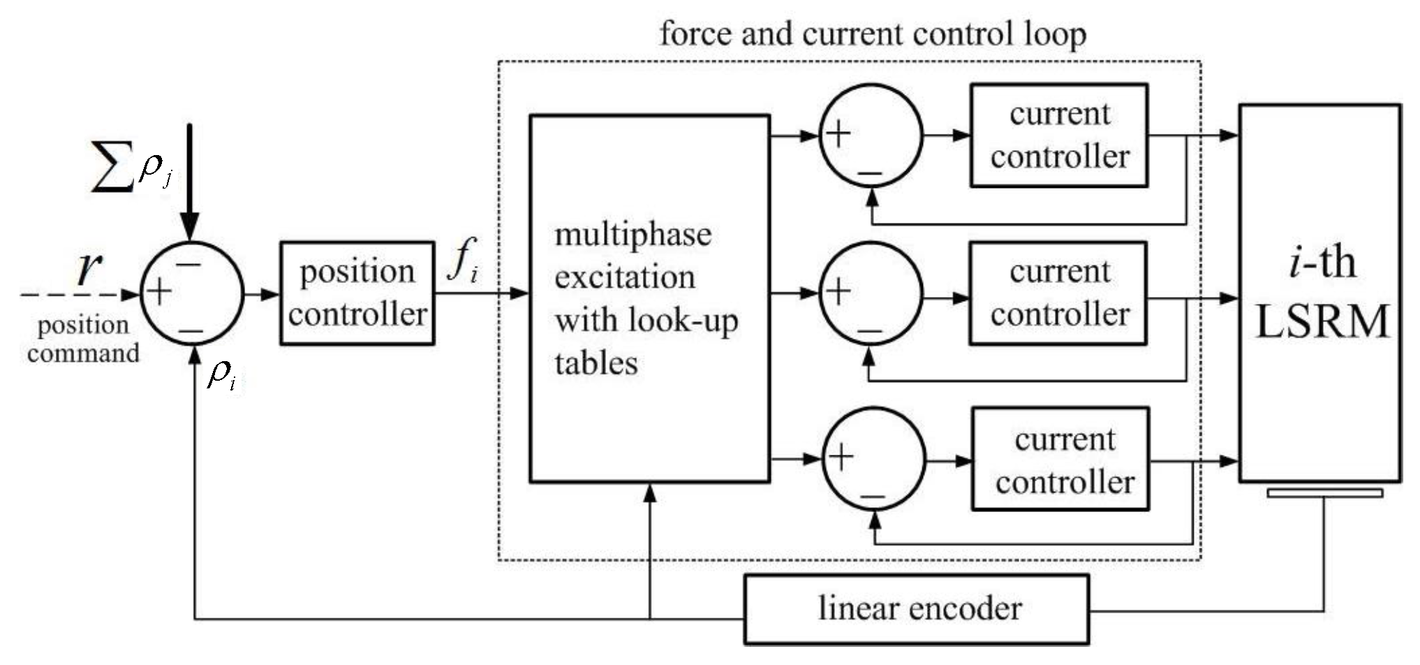
Any local LSRM control system is defined as an LSRM node in the LSRMs network. The control block diagram for any LSRM node can be depicted as shown in Figure 2. The LSRM node receives both the position feedback information from its linear encoder and the node , and only the leader node (i.e., the node located at the root of a certain spanning tree in a coordinated network topology) accesses the external reference information, i.e., the input signal of the LSRMs network from outside. Each LSRM node is composed of a local position controller, the multiphase excitation scheme with look-up table linearization, current controllers and an LSRM, and the control scheme conforms to the typical dual-loop architecture [28]. For the LSRM node , position error is decided from the difference between reference (the leader only) and actual position of the i-th LSRM, along with the position information from the LSRM node . The position controller then calculates the control input, and the multi-phase excitation with the look-up table linearizion scheme determines the current command for the k-th phase of the i-th LSRM, according to the current position of the i-th LSRM. Then, the current controller outputs the actual current to the k-th winding.
Rearranging Equation (3) in the state-space form, we have:
where is the control input of the i-th LSRM.
3. Synchronization Tracking Control Design
Since each LSRM is a mechatronic device fulfilling double-acting periodic line motion, some sinusoidal signals or its combinatorial patterns are often applied as the predefined trajectory planning some desired reciprocating motion for the LSRMs network. For this purpose, inspired by coupled harmonic oscillators synchronization proposed in [26,27], the distributed control law can be formulated as:
where is a parameter associated with the angular frequency of the reference sinusoidal signal. Substituting Equation (12) into Equation (11) , the LSRM node can be depicted as:
Let , , , the model of LSRMs network can be derived as:
According to Equation (14), the LSRMs network can be reformulated as:
where .
To prove the LSRMs network, Equation (15) has the ability to track a sinusoidal reference signal without phase disparity, and the following lemma is provided.
Lemma 1.
Let be the left and right eigenvectors of Laplacian matrix associated to the i-th eigenvalue , respectively. The eigenvalues of in Equation (15) can thus be represented as:
and its left and right eigenvectors can be denoted as the following:
Proof of Lemma 1.
We divide in two parts, denoted as and , respectively. For convenience, we omit the subscript index i or . For , we have:
Similarly, for , we have:
Likewise, we can obtain the equation as:
Substituting Equation (18a) into Equation (18b), we obtain:
In addition, substituting Equation (19a) into Equation (19b), we have:
According to Equation (21b), we notice , are the eigenvalue and left eigenvector of Laplacian matrix , respectively. Therefore, we have:
Equation (22) can thus be solved as:
In addition, from Equations (18a) and (19a), we know , . Lemma 1 is proved. ☐
Theorem 1.
Proof of Theorem 1.
According to [29], for a directed graph with a spanning tree in the network topology, its Laplacian matrix has the left eigenvector and the right eigenvector . They correspond to a simple zero eigenvalue of , and all rest of eigenvalues satisfy , where is the real part of a complex number. Furthermore, satisfies:
According to Lemma 1, the first two eigenvalues of in Equation (15) are , j is the imaginary unit. Accordingly, the left eigenvector and right eigenvector are , respectively. We have:
where
Here, is the Jordan block matrix associated to .
Since , , it follows that:
where is a block matrix of associated to and the simple zero eigenvalue of .
Let , the solution of LSRMs network in Equation (14) can be obtained as:
Moreover, according to Equation (26) :
According to Equation (24), it can be seen that can be set as in Equation (28). Therefore, Equation (28) is derived as:
where is the initial value of the LSRM node as the root of a directed spanning tree in the coordinated network topology , as shown in Figure 1. In addition, the states of LSRM nodes converge to the steady state as:
Obviously, the steady state values are determined by the initial values of root node . Therefore, the states of other LSRM nodes converge to the state of root without phase disparity. The fact verifies, under the effect of the coordinated control Equation (12), that the states of LSRMs network can track the state of root node represented as:
Letting , Equation (31) is rewritten as:
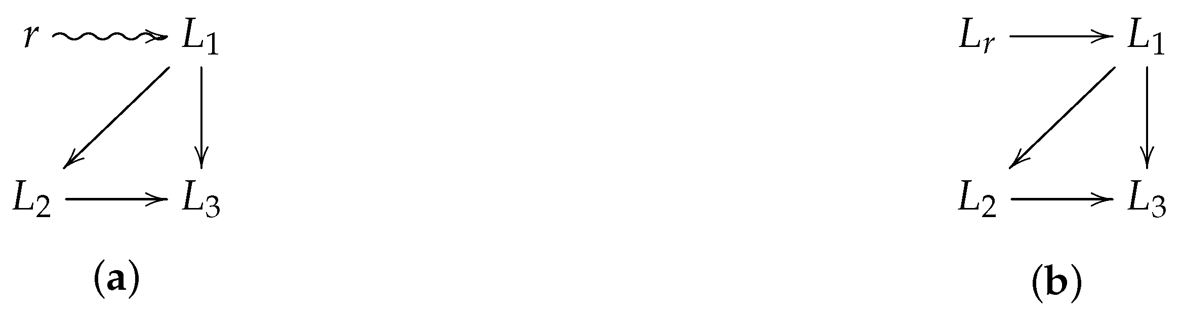
Accordingly, if the reference sinusoidal position signal in Figure 3a and its derivative is regarded as the state of a virtual root node , as shown in Figure 3b, the sinusoidal reference signal can be tracked asymptotically by the LSRMs network Equation (15) in a coupled harmonic oscillators synchronization manner . Theorem 2 is proved. ☐
Remark 1.
By selecting appropriate initial values of virtual root node , the LSRMs network Equation (15) can converge to the specified sinusoidal reference, which has phase and angular frequency .
4. Illustrative Examples
Example 1.
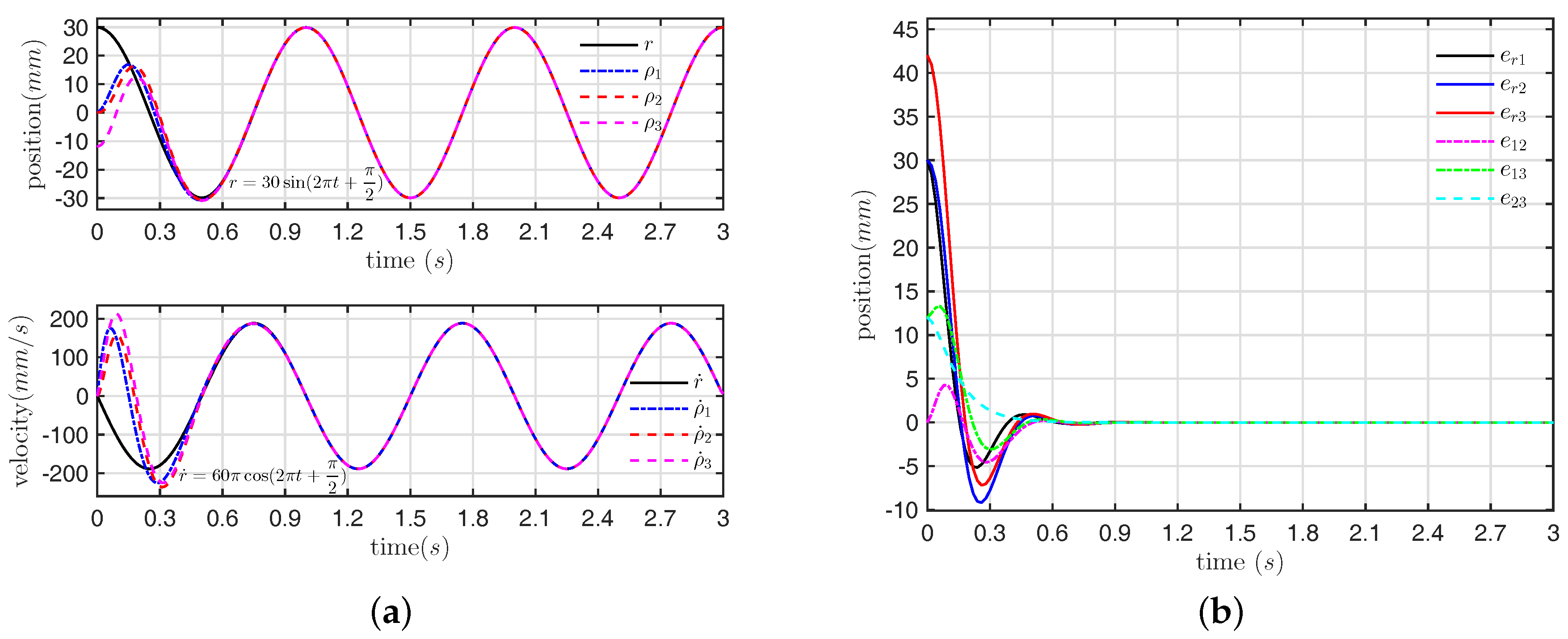
The sinusoidal reference r is modeled as a virtual LSRM node , and its initial phase and amplitude are , respectively. In addition, the angular frequency of is set as to investigate the system control feature tracking a higher frequency sine signal.
Each LSRM can be characterized by the second-order dynamics Equation (11). According to the method proposed in [8], system matrices and () can be obtained by the online least squares identification [4] with a sampling time of T = 0.001 s, and they can be derived as:
The initial positions of three LSRM nodes are set as , respectively, and all velocities of three LSRM nodes are 0. The control gain is set as 0.25 empirically (according to some parameter tuning experience). The topology of the LSRMs network is depicted as Figure 3.
The results of the state and position error responses are depicted in Figure 4a,b, respectively. Figure 4a illustrates that the LSRMs network Equation (14) tracks the reference in a zero phase-difference and asymptotic manner by applying the proposed control law Equation (12). The position errors among all nodes including are illustrated in Figure 4b. The disparity of position errors are eliminated for all LSRM nodes after about s.
Example 2.
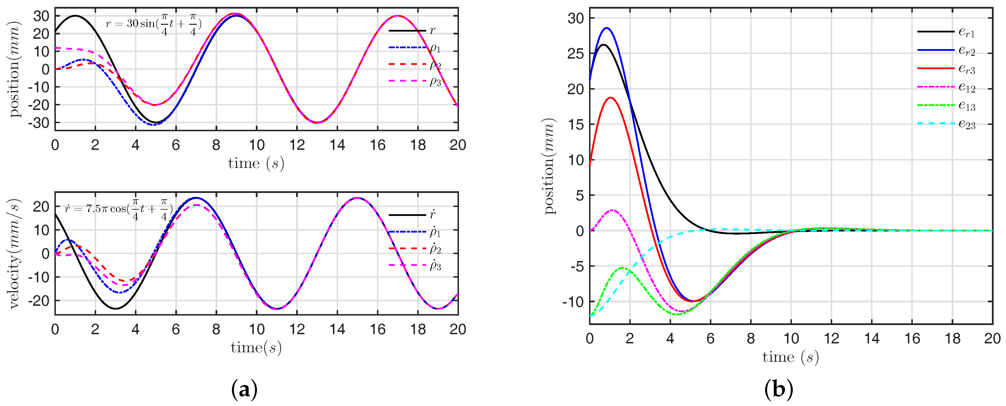
To further verify the effectiveness of the proposed control strategy, a comparative study with Example 1 is addressed. We locate the initial positions of three LSRM nodes at , respectively, and three LSRM nodes start work from static state. We set the reference r initial phase as , and the angular frequency are selected as to test the track feature to a lower frequency sine wave. The other systems parameters, such as the control gain, etc., are given the identical values as in Example 1.
The simulation results are shown in Figure 5a,b, respectively. The control performance from the proposed control method shows that a slower dynamic response can be achieved with a lower frequency sinusoidal reference, and compared to Example 1 for the same system without considering uncertain parameters and external disturbances. The results also demonstrate that the LSRMs network has successfully achieved the stable state without phase-difference after 10s. Therefore, the proposed tracking control scheme has certain superior stability.
Remark 2.
From two example comparative results, it is noted that the response effectiveness of Example 2 is counterintuitive, since the state consensus process of Example 2 takes a longer time rather than Example 1, as expected. The main cause is that the angular frequency of the reference sinusoidal signal strongly affects the response rate of each LSRM node through Equation (12).
5. System Construction and Experimental Results
5.1. System Construction
The experimental platform on the LSRMs network is exhibited in Figure 6. The platform applies an RT-LAB (OP5600) real-time digital simulator (Opal-RT Technologies, Montreal, Quebec, Canada) as the distributed controllers on each LSRM node, and builds a virtual LSRM node modeling the specific sinusoidal reference r. The position state of each LSRM node is measured and collected by a linear magnetic encoder and inspected by the host PC which is the management terminal remotely. The sampling frequency of the position control loop is 1 kHz. The current drivers of each LSRM node are connected to RT-LAB through the analog-to-digital converters. The current control is realized by three commercial amplifiers that are capable of inner current regulation based on the proportional-integral-differential algorithm with a switching frequency of 20 kHz. The sampling frequency of the position control loop is 1 kHz. The proposed distributed tracking control algorithm Equation (12) can be programmed under the MATLAB/Simulink (R2015a, MathWorks, Natick, Massachusetts, USA) environment, and the developed algorithm can be downloaded to the digital signal processor of RT-LAB. All control parameters can be modified online. The real time state response waveforms of all LSRM nodes of the LSRMs network are monitored and recorded by the host PC.
The control objects of three LSRM nodes are three identical LSRMs that conform to the switched reluctance machine structure. A double-sided machine arrangement guarantees a more stable and reliable output performance and the asymmetry of the stators ensures a higher force-to-volume ratio. The major machine specifications of the LSRM are demonstrated in Table 1 [28]. LSRM parameters can be obtained as , and through the online recursive least square parameter identification scheme.
5.2. Experimental Results
In order to validate the proposed control scheme based on coupled harmonic oscillators, the experiment of the tracking control is implemented for the LSRMs network based on the designed controller. Moreover, to compare with two aforementioned simulation examples, the system scenario and its parameters, including initial states of the reference and LSRM nodes and its controller gain, are given the same values as in Examples 1 and 2.
Figure 7a illustrates that the tracking control of three LSRM nodes takes the zero phase-difference effect at about the time of . From Figure 7b, the relative position errors among three LSRMs and the reference fall into in stable state after the transient time of .
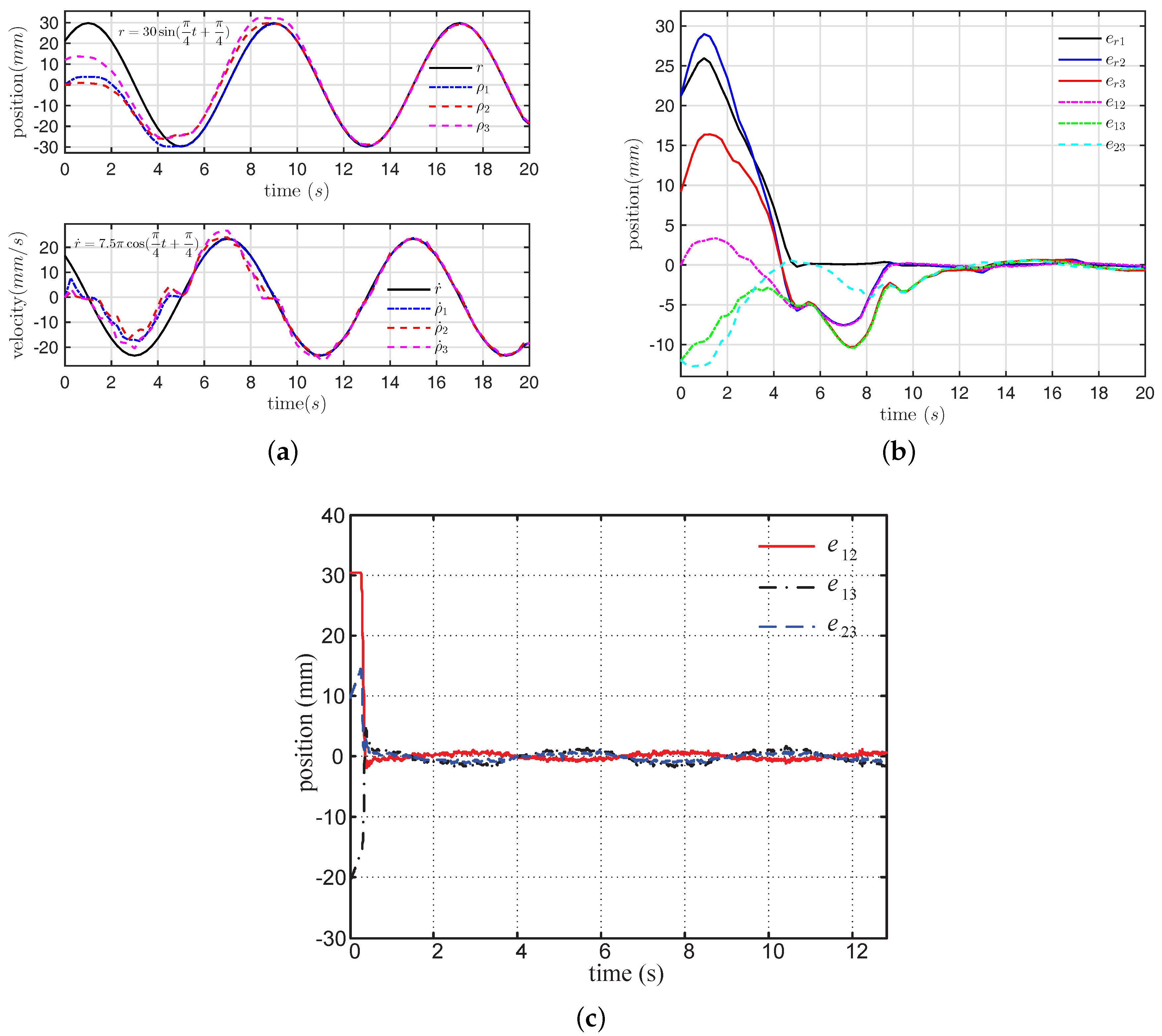
Figure 8a illustrates the dynamic position response waveforms under tracking control of three LSRM nodes. It is clear that the zero phase-difference effect is taken at about the time of . From the dynamic error response profiles as Figure 8b, it is clear that the maximum error values fall into at the steady state. Figure 8c is the steady-state position response profiles under the distributed PD control strategy [8]. It can be seen that the phase errors of the LSRMs network under the distributed PD control is greater than the phase-difference response from the proposed control strategy.
According to the tracking profiles of the three LSRMs in Figure 7 and Figure 8, the LSRMs network is all capable of following the position reference signal in zero phase-difference manner. However, the control performance from the three LSRMs is in disagreement and fluctuating slightly, especially in the steady state. This is mainly due to the imperfect manufacture and assembly of three LSRMs, which results in the asymmetric control performance from the positive and negative transitions. However, from Figure 4, Figure 5, Figure 7 and Figure 8, it can be seen that the tracking control effect displays high similarity to the aforementioned numerical simulative examples. It can be concluded that the proposed control method is effective.
6. Conclusions
A distributed control strategy of the LSRMs network is proposed for tracking a sinusoidal reference in a zero phase-difference manner. The dynamics of the LSRM nodes are modeled as general second-order linear systems by online system identification. Subsequently, inspired by the coupled harmonic oscillators synchronization, a distributed control is presented to track a sinusoidal reference without the phase-difference among each LSRM and the reference. Simulation and experimental results verify that the proposed control improves the synchronization and tracking accuracy performance of the LSRMs network through eliminating the phase-difference among LSRM nodes and virtual node modeling the sinusoidal reference. To further improve the tracking precision, it is suggested that the advanced internal model compensation schemes are introduced into the feedback control design of the LSRMs network. For the tracking control of some general periodical reference signals, the combined frequency domain analysis is also recommended for better control schemes. Furthermore, future work will also focus on the methods to annihilate load influence on the entire systems, including load influence on different topologies, dynamic load influence, etc.
Acknowledgments
This work was supported in part by the National Natural Science Foundation of China under Grant Nos. 51577121, 11572248, 51477103, 61690211 and 61403258. The authors also would like to thank the Guangdong and Shenzhen Governments under the Code of S2014A030313564, 2015A010106017, 2016KZDXM007 and JCYJ20160308104825040 for support.
Author Contributions
Bo Zhang and Jianping Yuan conceived and wrote the main body of the paper and designed the main body of study. J.F. Pan and Li Qiu guided the system design, analyzed the data and revised the manuscript. Wufeng Rao performed the simulations and experiments. Jianjun Luo and Honghua Dai helped to revise the paper.
Conflicts of Interest
The authors declare no conflict of interest.
References
- Leitao, P.; Marik, V.; Vrba, P. Past, Present, and Future of Industrial Agent Applications. IEEE Trans. Ind. Inform. 2013, 9, 2360–2372. [Google Scholar] [CrossRef]
- Qin, J.; Yu, C.; Gao, H. Coordination for Linear Multiagent Systems With Dynamic Interaction Topology in the Leader-Following Framework. IEEE Trans. Ind. Electron. 2014, 61, 2412–2422. [Google Scholar] [CrossRef]
- Amoros, J.; Andrada, P. Sensitivity Analysis of Geometrical Parameters on a Double-Sided Linear Switched Reluctance Motor. IEEE Trans. Ind. Electron. 2010, 57, 311–319. [Google Scholar]
- Pan, J.F.; Zou, Y.; Cao, G. Adaptive controller for the double-sided linear switched reluctance motor based on the nonlinear inductance modelling. IET Electr. Power Appl. 2013, 7, 1–15. [Google Scholar] [CrossRef]
- Lin, J.; Cheng, K.W.E.; Zhang, Z.; Cheung, N.C.; Xue, X.D.; Ng, T.W. Active Suspension System Based on Linear Switched Reluctance Actuator and Control Schemes. IEEE Trans. Veh. Technol. 2013, 62, 562–572. [Google Scholar] [CrossRef]
- Lin, J.; Cheng, K.W.E.; Zhang, Z.; Cheung, N.C.; Xue, X.D. Adaptive sliding mode technique-based electromagnetic suspension system with linear switched reluctance actuator. IET Electr. Power Appl. 2015, 9, 50–59. [Google Scholar] [CrossRef]
- Zhao, S.; Cheung, N.C.; Gan, W.; Yang, J.M.; Zhong, Q. Passivity-based control of linear switched reluctance motors with robustness consideration. IET Electr. Power Appl. 2008, 2, 164–171. [Google Scholar] [CrossRef]
- Zhang, B.; Yuan, J.; Qiu, L.; Cheung, N.; Pan, J.F. Distributed Coordinated Motion Tracking of the Linear Switched Reluctance Machine-Based Group Control System. IEEE Trans. Ind. Electron. 2016, 63, 1480–1489. [Google Scholar] [CrossRef]
- Qiu, L.; Shi, Y.; Pan, J.; Zhang, B.; Xu, G. Collaborative Tracking Control of Dual Linear Switched Reluctance Machines Over Communication Network With Time Delays. IEEE Trans. Syst. Man Cybern. 2016, 1–11. [Google Scholar] [CrossRef] [PubMed]
- Olfati-Saber, R.; Fax, J.A.; Murray, R.M. Consensus and Cooperation in Networked Multi-Agent Systems. Proc. IEEE 2007, 95, 215–233. [Google Scholar] [CrossRef]
- Cao, Y.; Yu, W.; Ren, W.; Chen, G. An Overview of Recent Progress in the Study of Distributed Multi-Agent Coordination. IEEE Trans. Ind. Inf. 2012, 9, 427–438. [Google Scholar] [CrossRef]
- Li, L.; Ho, D.W.C.; Lu, J. A Unified Approach to Practical Consensus with Quantized Data and Time Delay. IEEE Trans. Circuits Syst. I Regul. Pap. 2013, 60, 2668–2678. [Google Scholar] [CrossRef]
- Yu, W.; Chen, G.; Cao, M.; Ren, W. Delay-Induced Consensus and Quasi-Consensus in Multi-Agent Dynamical Systems. IEEE Trans. Circuits Syst. I Regul. Pap. 2013, 60, 2679–2687. [Google Scholar] [CrossRef]
- Wei, J.; Fang, H. Multi-agent consensus with time-varying delays and switching topologies. J. Syst. Eng. Electron. 2014, 25, 489–495. [Google Scholar] [CrossRef]
- Wang, H. Consensus of Networked Mechanical Systems With Communication Delays: A Unified Framework. IEEE Trans. Autom. Control 2014, 59, 1571–1576. [Google Scholar] [CrossRef]
- Liu, K.; Zhu, H.; Lu, J. Bridging the Gap Between Transmission Noise and Sampled Data for Robust Consensus of Multi-Agent Systems. IEEE Trans. Circuits Syst. I Regul. Pap. 2015, 62, 1836–1844. [Google Scholar] [CrossRef]
- Ning, X.; Yuan, J.; Yue, X. Uncertainty-based Optimization Algorithms in Designing Fractionated Spacecraft. Sci. Rep. 2016, 6, 22979. [Google Scholar] [CrossRef] [PubMed]
- Zhang, Q.; Lapierre, L.; Xiang, X. Distributed Control of Coordinated Path Tracking for Networked Nonholonomic Mobile Vehicles. IEEE Trans. Ind. Inf. 2013, 9, 472–484. [Google Scholar] [CrossRef]
- Dong, X.; Yu, B.; Shi, Z.; Zhong, Y. Time-Varying Formation Control for Unmanned Aerial Vehicles: Theories and Applications. IEEE Trans. Control Syst. Technol. 2014, 23, 340–348. [Google Scholar] [CrossRef]
- Cheng, M.H.; Li, Y.J.; Bakhoum, E.G. Controller Synthesis of Tracking and Synchronization for Multiaxis Motion System. IEEE Trans. Control Syst. Technol. 2014, 22, 378–386. [Google Scholar] [CrossRef]
- Li, X.; Wang, X.; Chen, G. Pinning a complex dynamical network to its equilibrium. IEEE Trans. Circuits Syst. I Regul. Pap. 2004, 51, 2074–2087. [Google Scholar] [CrossRef]
- Wang, X.; Su, H. Pinning control of complex networked systems: A decade after and beyond. Ann. Rev. Control 2014, 38, 103–111. [Google Scholar] [CrossRef]
- Cao, Y.; Ren, W. Distributed Coordinated Tracking with Reduced Interaction via a Variable Structure Approach. IEEE Trans. Autom. Control 2012, 57, 33–48. [Google Scholar]
- Wang, X.; Hong, Y.; Huang, J.; Jiang, Z. A Distributed Control Approach to A Robust Output Regulation Problem for Multi-Agent Linear Systems. IEEE Trans. Autom. Control 2010, 55, 2891–2895. [Google Scholar] [CrossRef]
- Wieland, P.; Sepulchre, R.; Allgower, F. An internal model principle is necessary and sufficient for linear output synchronization. Automatica 2011, 47, 1068–1074. [Google Scholar] [CrossRef]
- Su, H.; Wang, X.; Lin, Z. Synchronization of coupled harmonic oscillators in a dynamic proximity network. Automatica 2009, 45, 2286–2291. [Google Scholar] [CrossRef]
- Ren, W. Synchronization of coupled harmonic oscillators with local interaction. Automatica 2008, 44, 3195–3200. [Google Scholar] [CrossRef]
- Pan, J.F.; Zou, Y.; Cao, G. An Asymmetric Linear Switched Reluctance Motor. IEEE Trans. Energy Convers. 2013, 28, 444–451. [Google Scholar] [CrossRef]
- Mesbahi, M.; Egerstedt, M. Graph Theoretic Methods in Multiagent Networks; Princeton University Press: Princeton, NJ, USA, 2010; pp. 399–403. [Google Scholar]
Figure 1.
Topology of coodinated network.

Figure 2.
Control block diagram for the linear switched reluctance machine (LSRM) node.

Figure 3.
LSRMs network with the virtual LSRM modeling reference. (a) with reference; and (b) with virtual node.
Figure 3.
LSRMs network with the virtual LSRM modeling reference. (a) with reference; and (b) with virtual node.

Figure 4.
(a) Position and velocity response and (b) relative position error response.

Figure 5.
(a) Position and velocity response and (b) relative position error response.

Figure 6.
Experimental platform of LSRMs network. (1) LSRM 1; (2) LSRM 2; (3) LSRM 3; (4) linear encoder; (5) RT-LAB; (6) current amplifier; (7) power supply; and (8) connection interface to RT-LAB.
Figure 6.
Experimental platform of LSRMs network. (1) LSRM 1; (2) LSRM 2; (3) LSRM 3; (4) linear encoder; (5) RT-LAB; (6) current amplifier; (7) power supply; and (8) connection interface to RT-LAB.
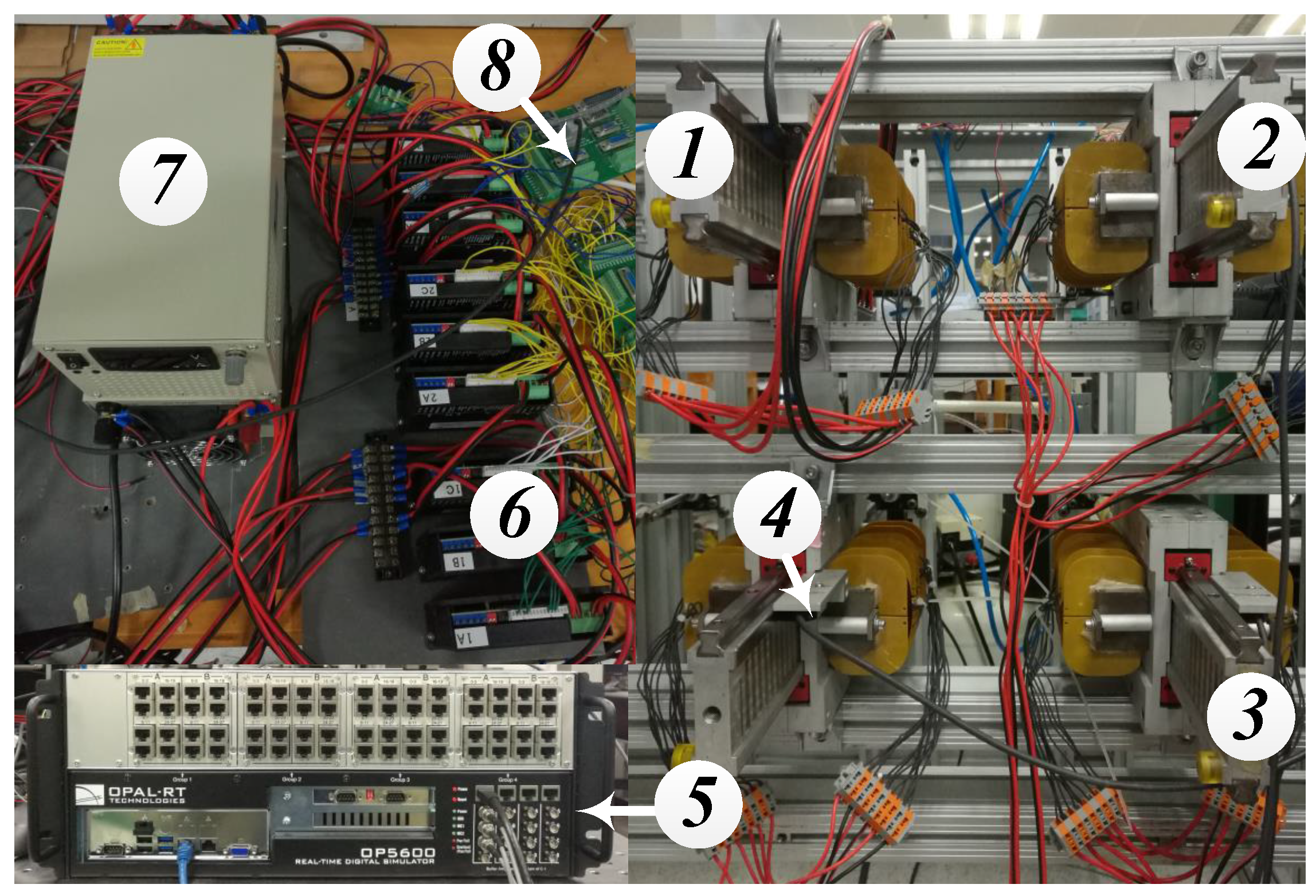
Figure 7.
Position and velocity of reference and three LSRMs corresponding with Example 1.
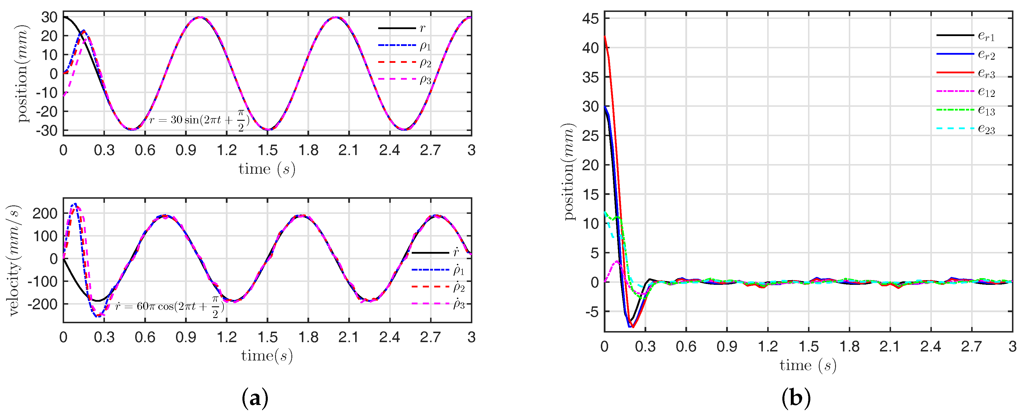
Figure 8.
Position and velocity of reference and three LSRMs corresponding with Example 2.


Table 1.
Main specifications of linear switched reluctance machine (LSRM).
| Quantity | Value |
|---|---|
| Mass of moving platform | 3.8 kg |
| Mass of stator | 5.0 kg |
| Pole pitch | 12 mm |
| Pole width | 6 mm |
| Air gap length | 0.3 mm |
| Phase resistance | 2 ohm |
| Number of turns | 200 |
| Stack length | 50 mm |
| Rated power | 250 W |
| Voltage | 50 v |
| Encoder resolution | 1 m |
© 2017 by the authors. Licensee MDPI, Basel, Switzerland. This article is an open access article distributed under the terms and conditions of the Creative Commons Attribution (CC BY) license (http://creativecommons.org/licenses/by/4.0/).
Share and Cite
MDPI and ACS Style
Zhang, B.; Pan, J.F.; Yuan, J.; Rao, W.; Qiu, L.; Luo, J.; Dai, H. Tracking Control with Zero Phase-Difference for Linear Switched Reluctance Machines Network. Energies 2017, 10, 949. https://doi.org/10.3390/en10070949
AMA Style
Zhang B, Pan JF, Yuan J, Rao W, Qiu L, Luo J, Dai H. Tracking Control with Zero Phase-Difference for Linear Switched Reluctance Machines Network. Energies. 2017; 10(7):949. https://doi.org/10.3390/en10070949
Chicago/Turabian StyleZhang, Bo, J.F. Pan, Jianping Yuan, Wufeng Rao, Li Qiu, Jianjun Luo, and Honghua Dai. 2017. "Tracking Control with Zero Phase-Difference for Linear Switched Reluctance Machines Network" Energies 10, no. 7: 949. https://doi.org/10.3390/en10070949
Note that from the first issue of 2016, this journal uses article numbers instead of page numbers. See further details here.