Article

Linking the Power and Transport Sectors—Part 2: Modelling a Sector Coupling Scenario for Germany

1
Institute of Electrochemical Process Engineering (IEK-3), Forschungszentrum Jülich GmbH, Wilhelm-Johnen-Str., 52428 Jülich, Germany
2
Chair of fuel cells, RWTH Aachen University, c/o Institute of Electrochemical Process Engineering (IEK-3), Forschungszentrum Jülich GmbH, Wilhelm-Johnen-Str., 52428 Jülich, Germany
*
Author to whom correspondence should be addressed.
Energies 2017, 10(7), 957; https://doi.org/10.3390/en10070957
Submission received: 29 March 2017 / Revised: 14 June 2017 / Accepted: 27 June 2017 / Published: 20 July 2017
(This article belongs to the Section F: Electrical Engineering)

Abstract

:
“Linking the power and transport sectors—Part 1” describes the general principle of “sector coupling” (SC), develops a working definition intended of the concept to be of utility to the international scientific community, contains a literature review that provides an overview of relevant scientific papers on this topic and conducts a rudimentary analysis of the linking of the power and transport sectors on a worldwide, EU and German level. The aim of this follow-on paper is to outline an approach to the modelling of SC. Therefore, a study of Germany as a case study was conducted. This study assumes a high share of renewable energy sources (RES) contributing to the grid and significant proportion of fuel cell vehicles (FCVs) in the year 2050, along with a dedicated hydrogen pipeline grid to meet hydrogen demand. To construct a model of this nature, the model environment “METIS” (models for energy transformation and integration systems) we developed will be described in more detail in this paper. Within this framework, a detailed model of the power and transport sector in Germany will be presented in this paper and the rationale behind its assumptions described. Furthermore, an intensive result analysis for the power surplus, utilization of electrolysis, hydrogen pipeline and economic considerations has been conducted to show the potential outcomes of modelling SC. It is hoped that this will serve as a basis for researchers to apply this framework in future to models and analysis with an international focus.

1. Introduction

Linking the power and transport sectors under the rubric of the so-called “Sector Coupling” (SC) approach as part of the effort to achieve greenhouse gas (GHG) emissions reduction goals is an on-going research topic. Whereas Part 1 [1] of this paper analysed the general principle of SC, reviewing some of the current literature and showing its potential for the power and transport sectors, this part of the paper will outline a detailed example for modelling SC in the power and transport sectors. In general, there are two possible approaches when modelling SC, namely a closed model environment and one that sums up different sub-models (Figure 1). Closed model environments aim to represent all sectors and technologies within one major structure [2,3,4,5]. They are used to illuminate general tendencies and hence necessarily simplify complex phenomena, but, on the other hand, are able to run on computers with limited capacities. Such simplifications could include, for example, that they do not use a detailed spatial resolution, but rather add up all the production and demand profiles to a single node. Model environments composed of different sub-models attempt to circumvent these disadvantages. For example, a sub-model could describe household demand with an in-depth analysis and give these results to a power-flow-model that considers the electrical grid and hence the power-flow in detail. On the other hand, calculations such as this require substantial computational capacities. Both modelling approaches have their value and have utility in answering the research question. A more in depth description of the challenges of modelling energy systems can be found in Pfenninger et al. (2014) [6]. Since a detailed surplus analysis is a key part of this paper, the authors adopted the approach of detailed sub-models of the power and transport sectors.
The model environment used (see Section 2) will give researchers an approach and a methodology for conducting similar analyses in different countries, such as that which was already conducted by Guandalini et al. (2017) [7]. As the focus of the literature review in Part 1 [1] was on Germany and the model environment is based on this country, a SC scenario for Germany will be developed. This scenario analyses the potential for linking the power and transport sectors via fuel cell vehicles (FCVs) and a dedicated hydrogen pipeline grid. Different uses of hydrogen, for example in the transport sector via power-to-fuel [8,9], steel production [10] or the linking of the heat and electricity sectors [11], the potential for reducing wind farm forecast errors [12], the use of hydrogen for methanation purposes [13,14] or as a feed-in to a natural gas grid [15], are not discussed in this article.
To achieve the CO2-reduction goals by 2050, a high share of renewable energy sources (RES) was assumed. The surplus power generated by these will be used to produce hydrogen via electrolysis as per the so-called “power-to-gas” approach. To demonstrate the necessary capabilities of SC models in terms of model parameters, the surplus analysis shows different spatial resolutions (see Section 3). Furthermore, the utilization of the electrolysis and the potential hydrogen pipeline network will be analysed in more detail. To demonstrate the economic feasibility of SC, an economic assessment for three different scenarios will be conducted.

2. The METIS Package

SC on a national scale and beyond requires computational resources and algorithm development, which, in general, constitutes a significant challenge and limiting factor to research efforts in this field. Therefore, before continuing with a discussion of the methodologies used in this study, a short description of our toolset is provided. In regard to data management, an MSSQL database was used, which provides data distribution across multiple hard drives, as well as optimized data retrieval procedures. All data analysed in this study, including the finalized hourly time series values of residual load in all German counties or municipalities, are stored within this database. For example, individual wind turbine locations across Germany in each of the constructed scenarios are also included.
The methodological formulation of the described model is constructed from an amalgamation of models developed by students and doctoral candidates working at the IEK-3 at the Forschungszentrum Jülich (Jülich, Germany) over the last few years (selection: [12,16,17,18,19,20,21,22,23,24,25,26]). Currently, these models correspond to a variety of environments; however, an effort has begun to implement all procedures in the Python programming language. We have designated this project METIS (models for energy transformation and integration systems). Moreover, the final project will also incorporate new and significantly improved methods to describe the model and will be suitable for performing analyses across all of Europe. Table 1 displays the sub-models used in the METIS environment and literature for a more detailed description of these packages. To give an overview of the most important steps in the METIS environment, the sub-models for the power and transport sectors will be described in more detail in the following sections.

2.1. The Power Sector

Specifically, the model decomposes the German power sector into two sub-regimes, namely electrical production and electrical load, both of which are determined at hourly resolution over a complete year and distributed across Germany’s 11,268 municipalities. The first regime, electricity production, is composed of both a subset of conventional power plants that are operating (or at least planned for operation) in Germany as of 2012 and a collection of RES, whose technology share, total capacity and spatial distribution has been set according to predetermined scenarios. The second regime, electrical load, considers the hourly aggregated load for Germany as reported by ENSOE-E [30], which has been corrected for missing demand sources [31] and is then distributed across the country in accordance with geospatial quantities. Between these two regimes is the electrical transmission network, which has been mapped in house on the basis of publically-available data [32].
Before a simulation begins, the hourly residual load of each sub-region is calculated by subtracting net electrical demand from renewable production of the predetermined capacity scenario. These values are then used during a simulation comprised of 8760 hourly optimizations of the electricity market in which the optimal dispatch of conventional generators, in terms of the marginal generation cost, is determined. Despite this attempt to reconcile electrical demand and production, there will always be a number of regions whose renewable production, or a part thereof, cannot be dispatched due to grid limitations. This residual load after considering these grid limitations is the power then available for hydrogen production. Before moving on to a discussion of hydrogen interactions, the procedures summarized here are discussed in greater detail.

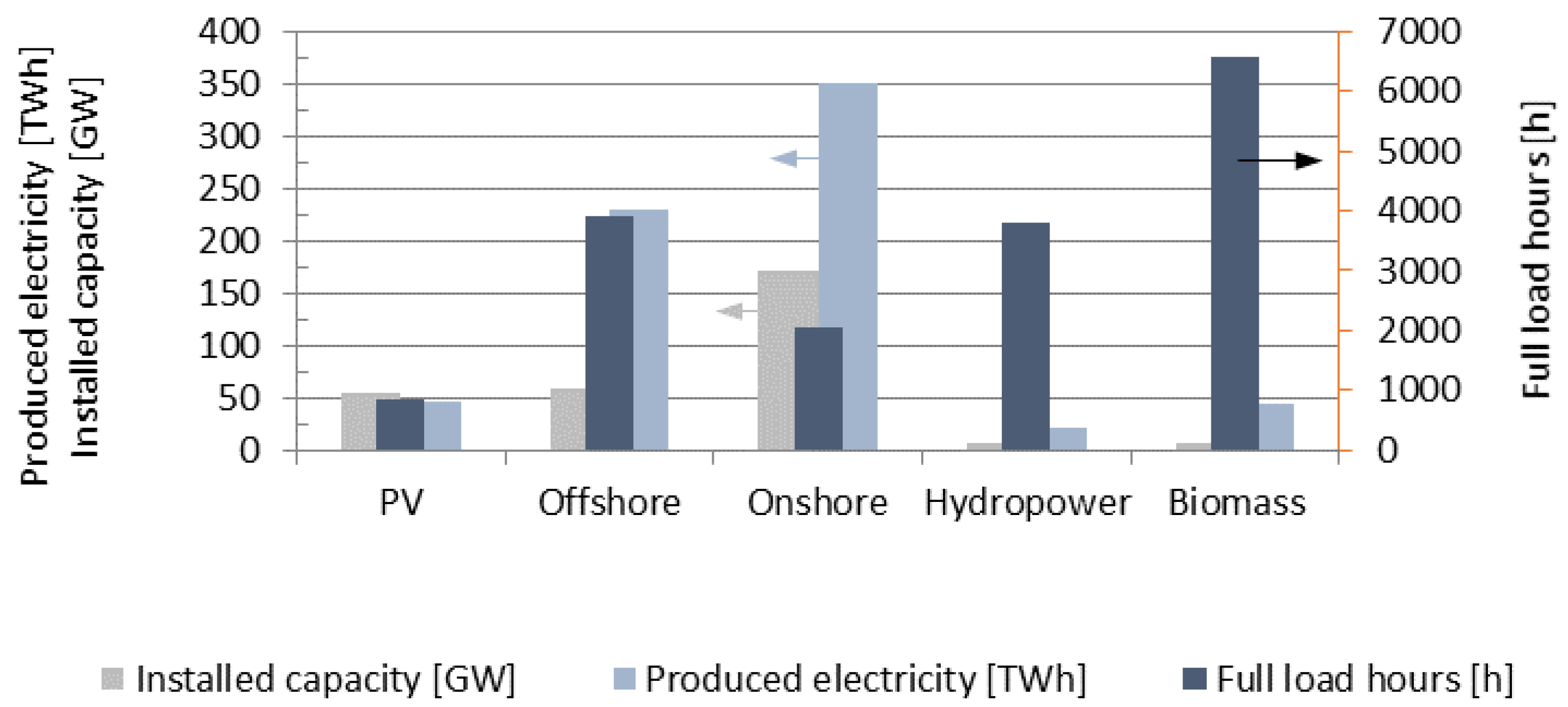
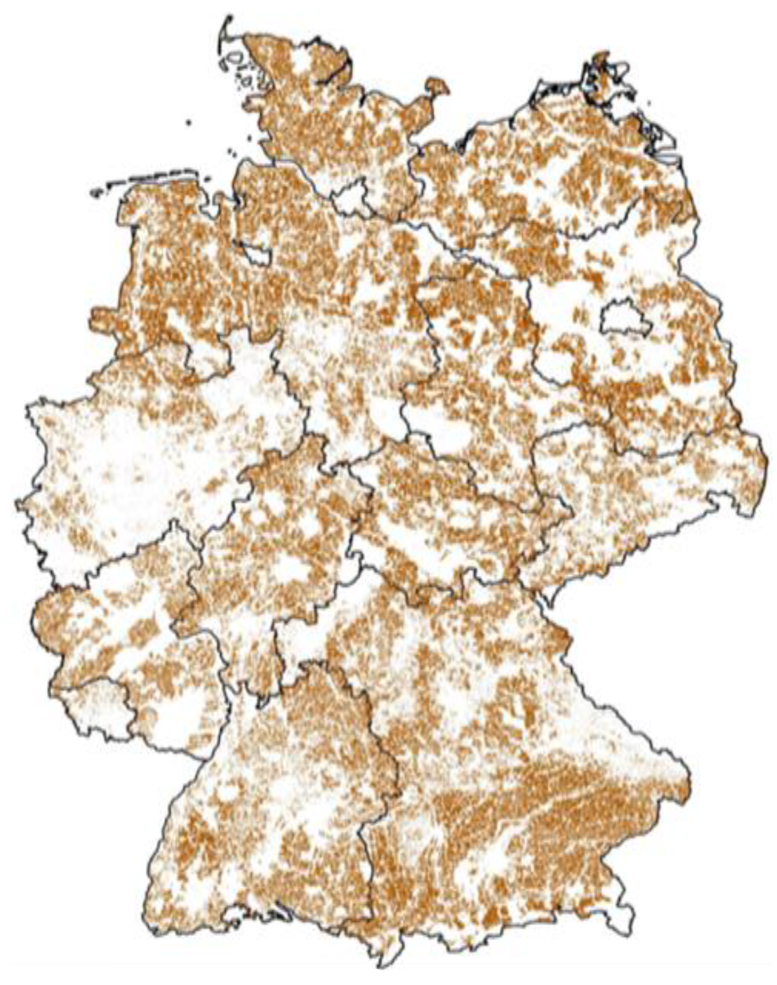
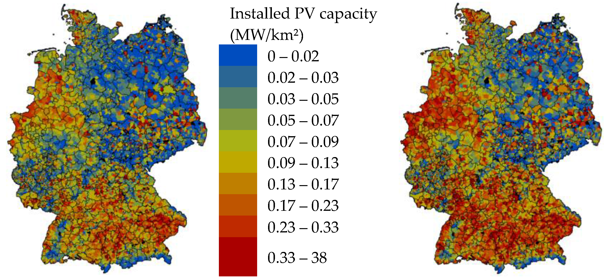
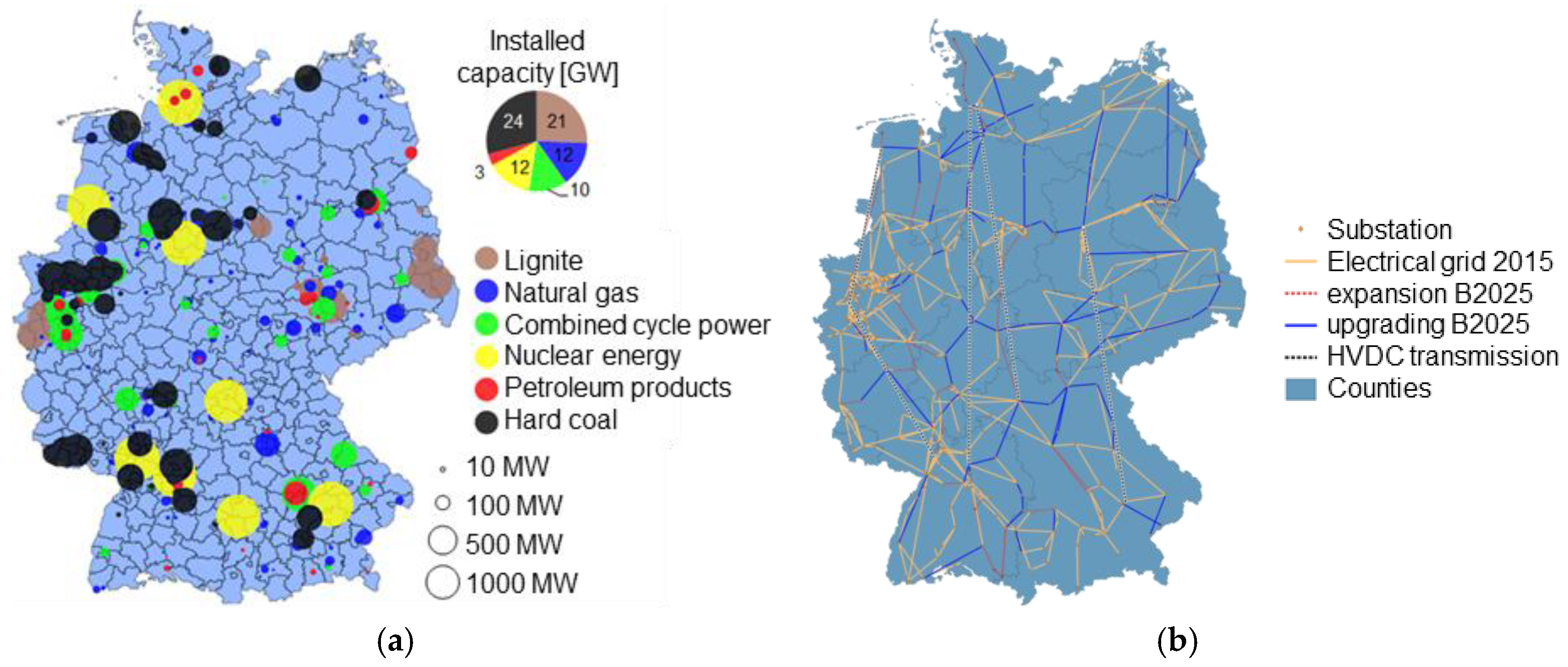
2.1.1. Renewable Capacity

In order to determine the regional hourly production from renewable generators, RES capacity scenarios must be generated prior to running a dispatch simulation. Furthermore, a single capacity scenario is comprised of individual resource capacity scenarios for each of the individual renewable technologies. These, in order of emphasis, are onshore wind, offshore wind, PV, hydropower and biomass. A final RES capacity scenario comprises a superposition of resource capacity scenarios. For reference, a sample capacity scenario was employed during our analyses, and is shown in Figure 2, wherein the installed capacity is depicted, along with the resulting energy production and average full load hours of each technology. The procedure for determining the regional distribution and subsequent production profiles for a single resource capacity scenario differs according to the resource in question, and so each of these is summarized in the following sections. In most cases, however, a detailed account of the full procedure is beyond the scope of this report; a full description can be found in Robinius (2015) [16].
Due to its vast potential in Germany’s northern regions, onshore wind is the primary RES focus in the described model. As such, the procedure for determining regional onshore wind potential is also the most detailed in comparison to the other RES options. This procedure begins by determining the land availability for wind turbines using the GIS software QGIS. By beginning with a blank slate of Germany (initially assumed to be comprised of 100% available land), individual pixels with a resolution of 100 m by 100 m are defined as inadequate on the basis of a number of constraints. The Corine Land Cover dataset [33] is used to subtract pixels that correspond to physically unsuitable land cover, such as urban areas, industrial areas, mountainous regions and cropland. The CDDA [34] is used to subtract regions that are nationally or internationally protected, including nature reserves, parks and protected habitats. Lastly, a combination of the previous two sources, as well as Open Street Map [35], is used to enforce policy-defined security distances from places such as roadways, airports and commercial zones. Areas that remain after the subtraction procedures constitute the land that is eligible for the placement of wind turbines. Figure 3 shows a result of this procedure, which was used in the analysis discussed in this report, in which eligible land is shown in brown and totals 113,115 km2 across Germany. Particularly noteworthy is the large amount of available land in the north, where wind potential is greatest.
Having acquired the available land for placing wind turbines, an optimized placement algorithm is used to determine specific latitude and longitude coordinates for the maximum number of turbines [16,21]. In addition to ensuring that all turbines are placed on eligible land, this algorithm assumes that no two turbines can be placed closer than 280 m apart (corresponding to 10 times a standard rotor diameter of the Nordtank 300 kW wind turbine). The purpose of this separation is to minimize wake effects on wind turbines that are down-wind of adjacent turbines [36]. A total of 1,652,827 potential turbine placements across Germany were identified.
Having established the coordinates of the maximal number of wind turbines across Germany, the distribution of any particular wind capacity scenario can then be evaluated. First, probability distribution functions (PDFs) for wind speeds at 80 m from each turbine location were interpolated from a dataset of Weibull distribution parameters at 200 m spatial resolution [37]. Using these PDFs in conjunction with four representative wind turbine power curves, an expected levelized cost of electricity (LCOE) for each turbine location can be calculated. Determining the distribution then becomes a matter of repeatedly searching for the best location amongst all available locations that promise the cheapest expected LCOE. On the first iteration of this search process, a turbine is placed at the most optimal location in Germany, after which this location is removed from the list of available locations and the next turbine is placed at the optimal location. This process continues until enough turbines have been placed, such that the desired wind capacity is satisfied. The final set of wind turbine locations is then stored for later use in determining regional residual loads.
In a similar fashion to onshore wind, offshore wind capacity scenarios are determined through the placement of wind turbines along the German coast in the North Sea. Therefore, the distribution of offshore wind turbines was readily found using the same algorithms developed for the onshore potential.
Next to wind, PV represents the second largest potential RES application in Germany [38]. A top-down approach was taken when determining the distribution of PV generation, which begins by accessing ENTSO-E’s time series data of Germany’s total PV production. These values, which are available at an hourly resolution, constitute the contribution of all PV generators across Germany. From this, hourly time series data are available for each county for the year and were selected from the ENSOE-E dataset. Moreover, these production values correspond to a capacity distribution of Germany’s total installed PV capacity during the chosen year [39]. In order to cast these values to a future capacity scenario, these distributed time-series values are then scaled such that the distribution’s installed capacity matches the desired capacity. To be certain that the scaled capacities in a municipality do not exceed the maximum potential, a detailed potential analysis similar to that for onshore wind has been conducted. According to the literature, the total capacity that can be installed ranges from 130 to 569 GW [40,41,42]. Due to the model’s restrictive assumptions, the possible installable capacity totals 117 GW. Figure 4 shows the spatial distribution of the installed PV capacity in 2014 and that projected in the model for the year 2050.
Despite its currently large contribution to RES production in Germany, hydropower is not expected to be a dominant renewable resource in the future [38]. For the most part, this is due to the nearly maximized utilization of hydropower sites across the country [43]. Therefore, only one hydro resource capacity scenario was constructed for these analyses, amounting to Germany’s currently installed hydro capacity of 5.6 GW. The distribution of this capacity across Germany was enabled by analysing rainfall patterns and distributing the ENSTO-E reported hydro production according to a single county’s rainfall in relation to all rainfall in Germany on an hourly basis.
Although it has continued to steadily grow in the last decade, RES production from biomass is not expected to contribute to the future energy mix. Like hydro, only one biomass resource capacity was developed for these analyses, amounting to Germany’s currently installed capacity of 6.41 GW. The energy map [39] provides a map of biomass production in Germany for the year 2013, and in a similar fashion to the previous procedures was used to distribute this capacity amongst each German county. Furthermore, these plants were utilized for 6556 full load hours in 2013 [38]. This equates to an installed capacity of 4.99 GW operating at full capacity at all times. Therefore, the final biomass distribution amounts to this reduced capacity and acts as a baseload with constant output for the entire year. In future, the biomass capacities could be optimized on the basis of the behaviour of the RES. This would minimize both the surplus and need for controllable power plants, but to a negligible extent.

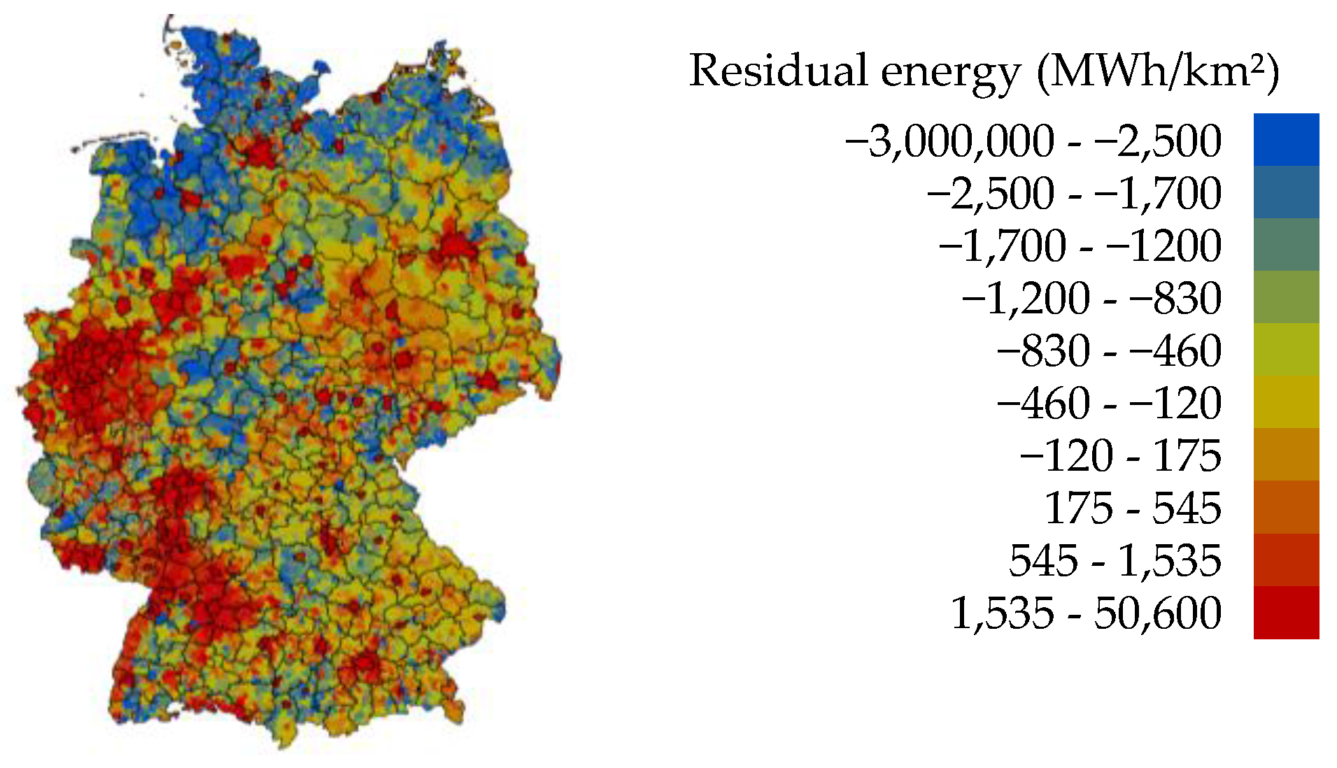
2.1.2. Residual Load

With a particular capacity scenario in hand, the next major task of the described model is to determine the residual load for each German municipality before the dispatch of conventional generators and grid dynamics are included. The process begins with a top-down approach for determining the electricity demand of each municipality at hourly resolution. Then, the RES generation within each municipality is determined according to the chosen scenario and subtracted from the electrical demand. As a result, hourly time series values of residual load are left over for each municipality.
Distributing electricity demand begins by collecting hourly demand values from the ENTSO-E database at the transmission system operator (TSO) level in Germany [30]. Each of these TSO-wide values is then distributed amongst the municipalities according to, e.g., mean GDP per capita in proportion to the sum of all GDP values. However, the values obtained from the ENTSOE-E database do not contain some important usages of electricity that must be included, such as industrial on-site electricity generation, the operation of electric trains and grid losses [44]. This can be seen by summing the annual demand from the four TSO from 2013, totalling 463.1 TWh and comparing this value to the reported German electricity demand of 527.9 TWh [45]. Therefore, the distributed electricity load values are corrected in order to account for this mismatch. Operating on the assumption that this unaccounted for electricity usage is uniformly distributed across the country, a uniform base load of 7.4 GW, distributed according to each county’s proportion of mean GDP per person was added to the hourly demand of all German counties and is constant throughout the year.
The next step in the process is to determine the RES electricity production values of each county according to the selected RES capacity scenario. As mentioned previously, time series values for PV, hydro and biomass are readily available from the results of developing these individual resource capacities. However, in the case of on-shore and off-shore wind, there is still more to do. For on-shore wind, development of the resource capacity scenario yields a list of wind turbine placements across the German countryside. By using historical wind speed data measured at 403 weather stations non-uniformly distributed across the country, power production values are calculated for each turbine according to the data of the closest weather station and the turbine’s power curve. Instead of using raw wind speed data for power calculations, however, the wind speed values are corrected for each wind turbine, such that the average of the wind speed data at that location corresponds to the expectation value of the associated Weibull distribution used during the capacity distribution process. Finally, all turbines production values contained within a municipality are aggregated for each. As before, the process for generating production values for offshore wind constitutes a simplified version of that for onshore wind. As with onshore, the development of the offshore capacity scenario provides suitable coordinates for individual wind turbines. There is not as much weather station data for offshore locations; however, there is also less expectation of variance between locations. As a result, the production values of all offshore wind turbines are conducted using a single wind speed dataset. The aggregation of individual offshore turbine production values is also performed; however, in this case, individual offshore turbine plants are treated as regions that are thought to have zero electricity demand.
Following these procedures, the residual load for each municipality can be calculated. This is performed by simply subtracting from each country’s electricity demand the production values from all RES producers in that municipality. A sample result of this is shown in Figure 5. The values depicted in this figure represent the load that remains after each municipality attempts to satisfy its own electricity demand. Although there may be some rare instances in which a county’s instantaneous load and demand offset each other (as seen in Figure 5 for the eastern part of Germany), the majority of the time there will be a discrepancy. These mismatches will either result in a positive residual load, referring to instances in which RES production is not enough to completely satisfy electrical demand, or a negative residual load, referring to instances in which a county is producing more RES electricity than it requires. After this point, the model’s objective is to simulate conventional dispatch and grid flows with the goal of, as much as possible, distributing RES electricity from counties with negative residual loads to those with positive residual loads or, failing this, to employ conventional generators to ensure that all counties have their electrical demands met.

2.1.3. Power Trading and Conventional Dispatch

To consider the electricity flows in the electrical grid, the model includes a transmission and dispatch optimization for every hour in the modelled year. In addition to the previously calculated residual loads that must be satisfied, this optimization requires detailed information about the electrical grid nodes, as well as the transmission capabilities, number and type of conventional generation sites contained within each district, and finally the import and export requirements between Germany and its neighbouring countries. Due to the limited number of nodes and computational restrictions, the residual load at the municipality level was summarized at the county level.
The grid itself was recreated according to the German grid development plant [32], which includes transmission lines at 380 and 220 kV, in addition to high voltage direct current transmission (Figure 6b). For the purposes of this study, all lines are assumed to operate with a loss of 0.055%/km [31]. Furthermore, the type and location of all power plants is based on information from the German Bundesnetzagentur (Figure 6a) [46], which provides a list of all power plants with a nominal capacity above 10 MW and includes, amongst other details, the federal state in which the plant was built, as well as its capacity, fuel type and year of first operation [31,47]. With the current plan of phasing out nuclear plants, in addition to reducing overall GHG emissions, the German energy mix will change rapidly in the coming years. To reflect this, the model allows for the selection of a subset of the power plants that are currently in operation, thus creating a conventional resource capacity scenario. For example, in accordance with German policy, all nuclear plants have been filtered out of the final analyses. In order to calculate a marginal cost for each power plant, an in-house analysis was performed to estimate the operating efficiency as a function of plant type, age and fuel cost, in addition to applying an optional carbon tax for all plants. Finally, to account for the import and export of energy to surrounding countries, the model also incorporates historic transfer values from a number of different sources [48,49,50,51,52,53,54,55]. Historical values were used in this case in order to avoid an overly complex scenario-space in which the residual load would need to be determined for all surrounding countries. Nevertheless, this approach was shown to provide reliable results [19].
Once all of the required pieces are available, the optimization procedure can begin, which, for the purposes of our analyses, was performed using MatLab’s linear optimization toolbox. Conversion to a Python power flow model is an on-going process. The overall objective of this optimization is to ensure that all counties ultimately feature zero or negative residual load, while also minimizing the cost, with respect to the marginal production price of conventional utilization without exceeding grid limitations. This second objective can also be thought of as a maximization of the available excess RES production inasmuch as the grid will allow, since counties with negative residual load are treated as power plants that have zero marginal cost. For each hour in the year, a unique linear program (LP) is constructed, which contains information regarding the available power plants, counties with negative residual load, losses associated with transferring power between any two grid nodes, maximal line capacities and the power requirement of all counties with positive residual load. As mentioned previously, a complete description of this procedure is beyond the scope of this report; however, more information can be found in Robinius [16]. Solving this LP provides, for the hour in question, the utilization of each power plant, the transfer of power between any power plant (or county with negative residual load) and any other county, as well as individual line usages. Most importantly, those counties that have retained a negative residual load despite the grid interactions are identified in addition to the time and magnitude of this excess. These are the optimal locations to consider when placing an electrolysis plant or hydrogen pipeline.
The main drawback to the described procedure worthy of discussion is that each hour is handled independently of the others, and as such there is, as of now, no way to account for the ramp-up time of power plants. This is not a problem for fast-acting plants such as combined cycle gas turbines (CCGT), but is potentially an issue for power plants with ramp rates longer than an hour. This issue is an on-going process within the model’s extensions for an upgraded version.
Now, a detailed description of the model environment in the transport sector will be described.

2.2. Transport Sector

Whereas “Linking the power and transport sectors—Part 1” [1] presents a detailed analysis of the status and goals in Germany for the transport sector, this section describes a modelling approach for SC. In future, there will be a high share of electric vehicles (EV), including battery electric vehicles (BEV) and FCVs. The spread depends on many factors, such as acceptance, costs, infrastructure and so on. To show the possibility of a hydrogen infrastructure, a high share of FCVs in the year 2050 is assumed. Therefore, BEVs will not be considered in further detail here.

2.2.1. Hydrogen Demand 2050

This section deals with the modelling of hydrogen sale on the district level. For that to happen, the assumed hydrogen sale is affected by two modelling parameters over the passage of time: the number of presumed FCVs, as well as by hydrogen use per vehicle. The assumed development of the FCV fleet orients itself through the extension of pathways to the year 2033 of H2 Mobility, whereby the given planning years are shifted by two years into the future [56,57,58]. Six companies and five associated partners from the automobile, gas and oil sectors joined forces to found the H2 Mobility. Their common goal is to put in place the infrastructure to guarantee nationwide hydrogen-powered mobility in Germany.
The maximally attainable share of hydrogen vehicles in the total car stock is assumed to be 75% in 2050 [59]. These sampling points are fitted to an S-Curve representing the lifecycle progress. The integration of the S-Curve as a special lifecycle type can be gleaned from Höft [60].
The vehicle’s annual mileage is set to 14,000 km [61] and its lifespan to 12 years [62]. Because of the expected compensation of market growth by prospective alternative mobility concepts like car sharing, it must be assumed that the total car stock of 44 million in 2014 will not increase [63]. The presumed hydrogen consumption is extrapolated linearly from 1.1 MJ/km or 0.92 kg per 100 km in 2010, respectively, to 0.7 MJ/km or 0.58 kg per 100 km in 2050, respectively, corresponding to development in accordance with the “moderate” scenario of the GermanHy study [59]. This procedure appears to show a realistic development of fuel consumption, since some vehicle manufacturers, such as Toyota (Mirai), already show consumption figures of 0.76 kg/100 km derived from 0.69 kg/100 km urban and 0.8 kg/100 km extra urban according to the EU2015/45ZY policy [64].
Figure 7 depicts the quantities of FCVs derived from boundary conditions and the resulting hydrogen consumption for vehicle supply. In contrast to the s-shaped trend of the FCV quantity, demand for hydrogen hits its peak of 2.93 million tons in 2052 and decreases continuously to 2.86 million tons in the year 2100. This effect can be attributed to new registrations of FCVs with higher efficiency.
Furthermore, Figure 7 depicts the number of FCVs according to Keles et al. [65] for the Lead scenario, as well as for Scenario 3. Keles et al. [65] used an agent-based model that allows the calculation of interdependencies between initial infrastructure, subsidies and tax abatements for FCVs. The “Lead scenario” and the “Scenario 3” are composed of [65]:
Lead scenario:
  • 500 hydrogen filling stations at the outset of the transformation in six metropolitan areas: the Ruhr area, Berlin, Hamburg, Munich, Stuttgart and Frankfurt.
  • Consumers are willing to pay €2000 more for “green technology”, namely FCVs, over petrol- or diesel-driven cars
  • No value added tax on FCVs in the beginning
  • Tax-free hydrogen for up to 500,000 FCVs
  • The same specific tax for hydrogen as for petrol and diesel for 1 million or more FCVs
Scenario 3:
• In contrast to the “Lead Scenario”, this scenario assumes equal taxes on hydrogen and petrol or diesel, respectively, at the outset of the infrastructure
Thus, this scenario assumes an absence of tax abatements for hydrogen.
The analysis confines itself to the years 2013–2040. As shown in Figure 7, it becomes apparent that under the assumed terms of the Lead scenario, the number of FCVs could increase sooner than in the METIS model. Thus, it appears that the development of FCVs in the METIS model does not represent the upper range of all possible prospective developments.
The accumulated hydrogen sale and FCVs are allocated at the district level by the following weighted indicators:
  • Population status
  • Site-specific population density
  • Obtainable private household income data per inhabitant
  • Inhabitant-related motor car density
  • Number of motor cars
Figure 8 demonstrates the hydrogen demand in 402 German districts in 2040 and 2052, the year of predicted peak demand. In 2040, the six districts with the highest projected hydrogen demands are Berlin, Hamburg, Munich, Hannover, Cologne and the Rhine-Sieg area, with 26, 17, 16, 12, 10 and 8 million kg per km2, respectively. This order does not change until 2052, with demand increasing to 77, 50, 46, 36, 30 and 22 million kg per km2, respectively.

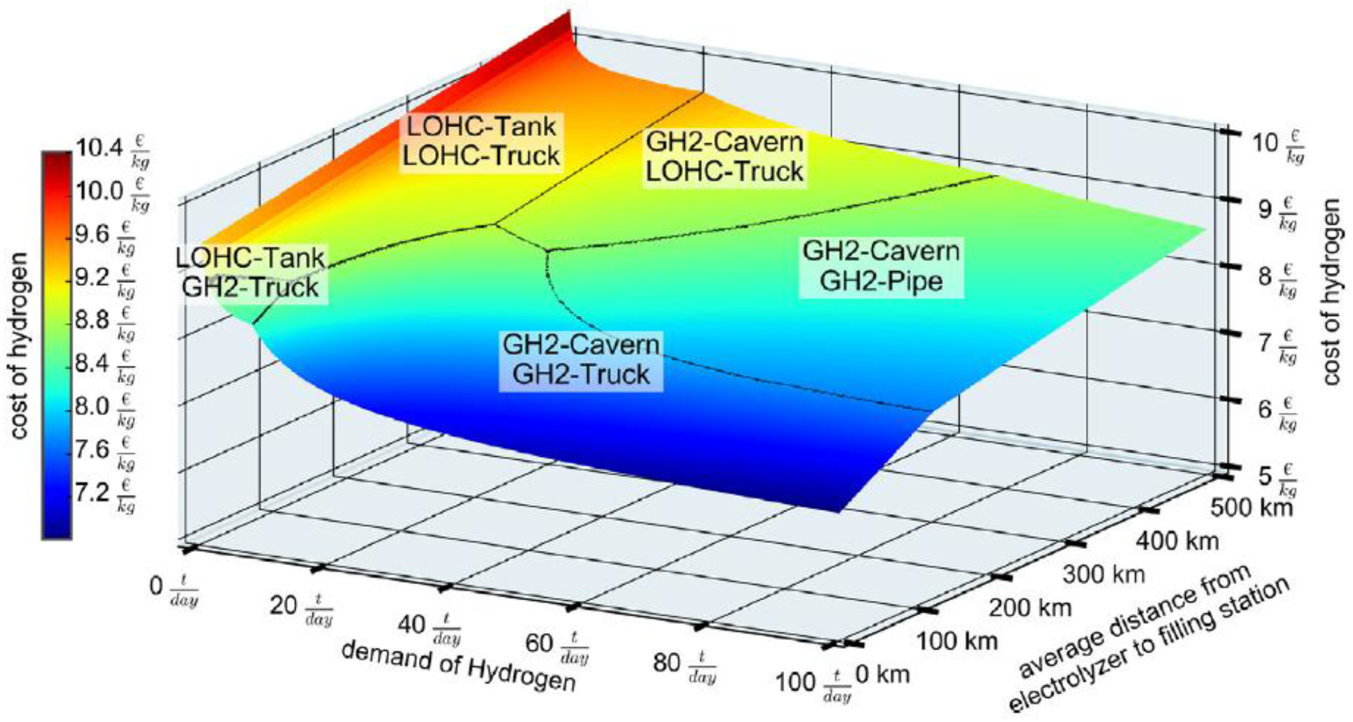
2.2.2. Hydrogen Transport

There are many different potential supply chains and costs for a hydrogen refuelling station (Figure 9). Nevertheless, for a high demand and a distance with more than 300 km, a hydrogen pipeline is the cheapest solution.
The methodology of calculating hydrogen pipelines is derived from the work of Grüger [67], Krieg [29] and Baufumé et al. [26], respectively. Within the scope of the latter, the shortest distance between sources—coal gasification and offshore wind farm aggradation areas—and sinks—9860 filling stations—are determined via existing lines. In doing so, the existing lines of the high pressure natural gas grid and rail network are used as potential routes for the grid of hydrogen pipelines. Without taking these input routes into consideration, the shortest connection between the source and sink would, for instance, move through an integral natural reserve [29]. Krieg [29] distinguishes between the transmission and distribution grid [29]. A transmission grid connects the sources and so-called hubs. These hubs represent secondary sources and are allocated to the centroid of the 413 analysed district areas within the scope of the modelling. Subsequently, the line length and line costs of the transmission grid are minimized through the use of a Dijkstra algorithm and genetic algorithm [29]. The 413 districts that are deposited within the model of Krieg [29] do not match the 402 districts in this model because of a local government reorganization, within which districts have been merged and hence it has been adjusted. Therefore, on the basis of the number of cars in the respective districts, hydrogen consumption in the 402 districts from Section 2.2.1 is allocated to the 413 districts to ensure the comparability of this work and that of Krieg [29]. This leads to the fact that the district Vorpommern-Greifswald contains three hubs that are located in the former districts of Greifswald, Ostvorpommern and Uecker-Randow.
In contrast to the transmission grid, the calculation of the distribution grid determines the direct connection between the source (the Hubs) and sink (the filling stations). Filling stations located along freeways are directly connected to the grid, whereas district filling stations are connected according to their calculated demand. If freeway filling stations are unable to satisfy the district’s demand, additional filling stations will be connected in the following order: firstly, filling stations are connected in metropolitan areas, then in urban areas and, finally, in rural areas. Filling stations are connected on the condition that the overall grid is the most favourable. Hence, in the case of doubt, filling stations are not always connected radially around the source ([29,67]) and for the modelling of this a Prime algorithm is implemented.
The exact input values of the modelling, such as the cost function or the hydrogen demand per district, depend on the analysed scenario.
Krieg [29] calculates three cost functions, namely “minimal”, “medium” and “maximal”, which consider both the piping costs of the hydrogen pipeline and the compressor costs, and these are compared in Figure 10 [29]. These cost functions are accordingly employed for the purpose of calculation.
Furthermore, the potential daily sale of a filling station is another element to determine the number of filling stations that must be connected to the distribution grid. On the basis of 9860 filling stations and an annual overall consumption of 5.4 million tons of hydrogen, Krieg [29] calculates 1500 kg per day and filling station. In order to maintain an adequate supply, the daily quantities of sale per filling station are adjusted to 803 kg per day according to the new overall consumption of 2.93 million tons.

3. Results Analysis

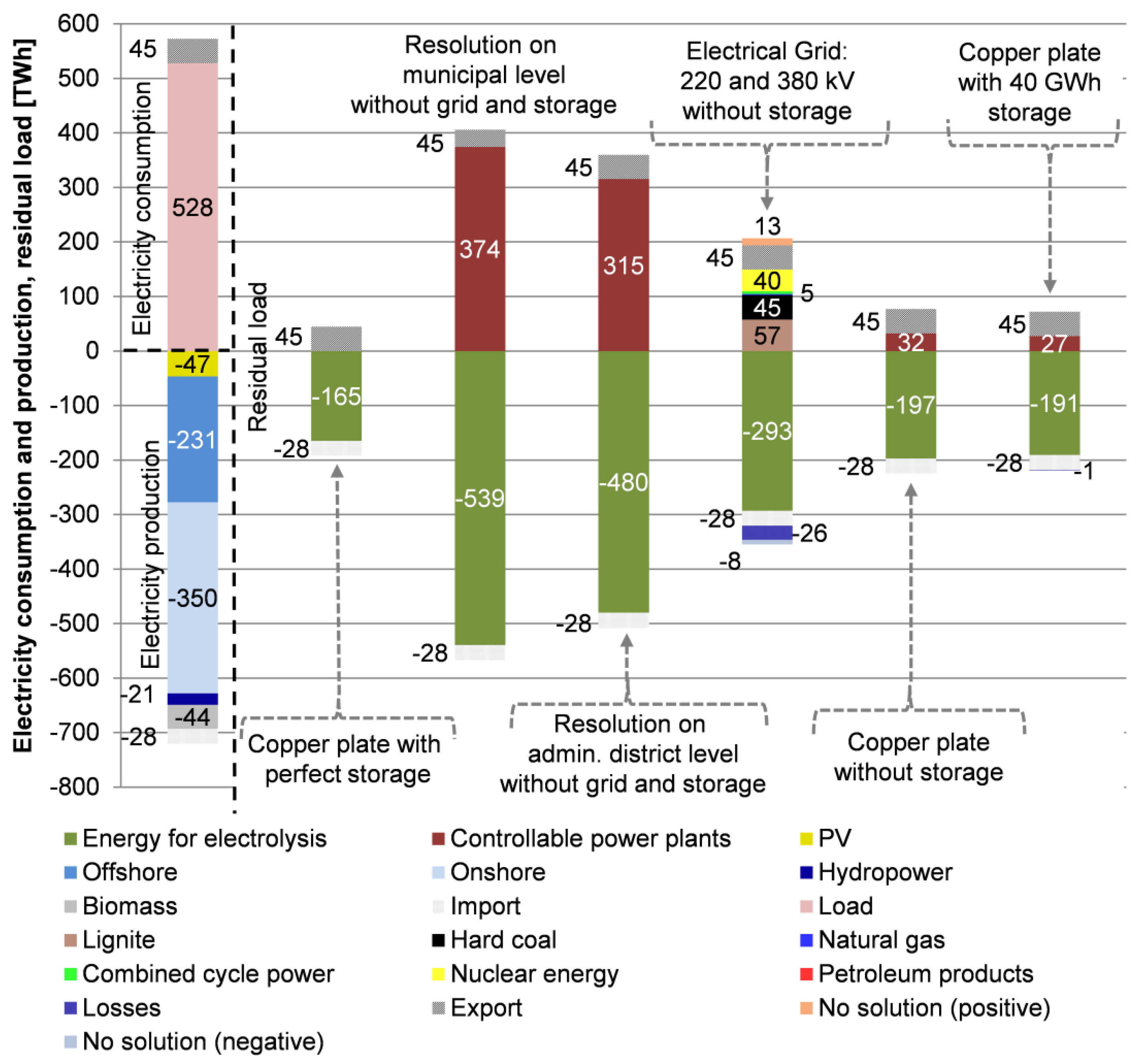
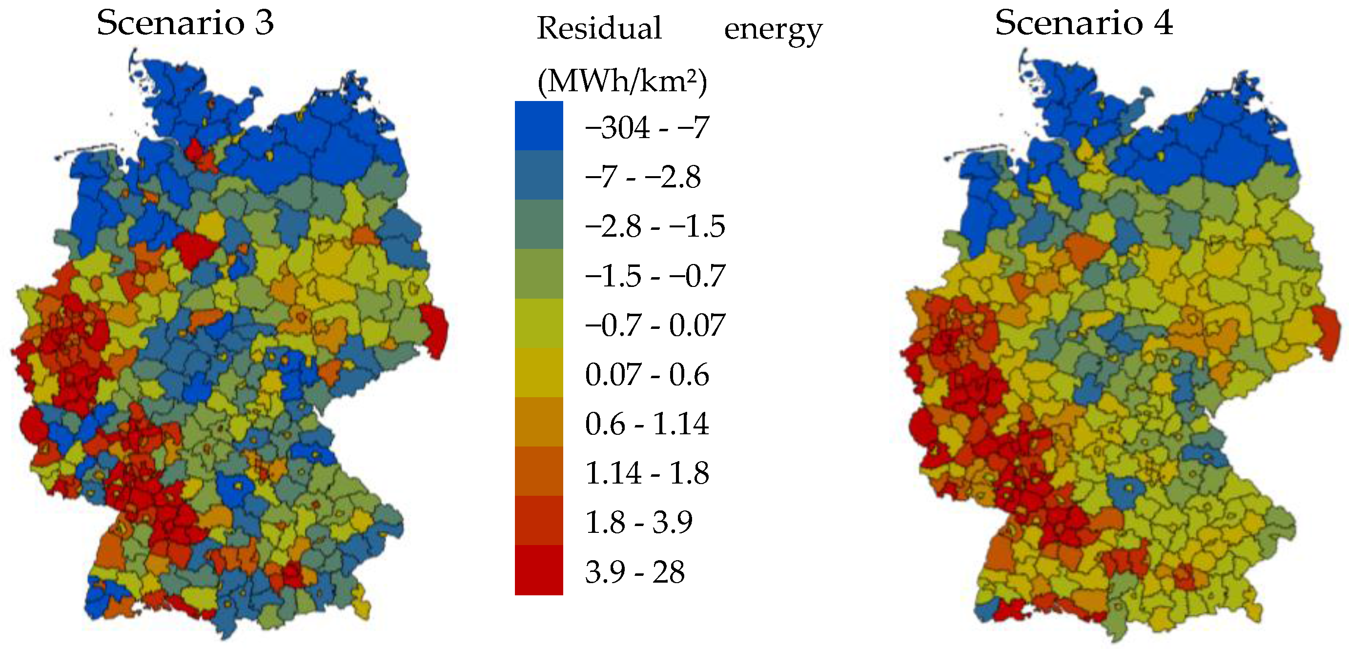
3.1. Surplus Analysis

The surplus depends on numerous input data, methodologies and assumptions, such as the spatial resolution of the model, the spatial distribution of the RES, the applied storage systems, the electrical grid topologies or the used power-to-X applications. These input data must be described in order to compare the results to other studies or show the limitations of the model. Whereas the spatial resolution in the METIS packages in terms of RES modelling or residual load analysis without considering the electrical grid is on the level of 11,268 municipalities in Germany (see Section 2.1.2), it changes on the level of 402 counties considering the electrical grid. To show the range of the potential surplus on the considered installed capacities of the RES (Figure 2), six different scenarios are applied:
  • Copper plate (no grid limitations) and perfect storage systems (no storage losses or limitations)
  • No electrical grid and no storage systems on the municipality level
  • No electrical grid and no storage systems on the county level
  • Current electrical grid (380 and 220 kV), no storage systems and current conventional power plants on the county level
  • Copper plate (no grid limitations) and no storage systems
  • Copper plate (no grid limitations) and 40 GWh of pumped storage hydropower stations (current situation in Germany)
Furthermore, to show the potential of possible power-to-X applications or the SC potential, and therefore the potential of linking the power and transport sectors, no power-to-X applications are considered at this point in the analysis. Figure 11 shows the electricity production, electricity demand and residual energy under these six different scenarios.
The surplus amounts of the scenarios amount to:
(1)
165 TWh
(2)
539 TWh
(3)
480 TWh
(4)
293 TWh
(5)
197 TWh
(6)
191 TWh
This shows that even after the physically impossible consideration of a “copper plate” and no storage losses or limitations, a surplus of 165 TWh will be produced and therefore a possibility of power-to-X applications is given. Furthermore, the results show that the spatial resolution of the model influences the surplus significantly. Going from the municipality to the county level, the surplus reduces from 539 to 480 TWh (Delta: 59 TWh). In both cases, only the accumulation of the residual load has been conducted. This underlines that the RES are highly spatially distributed and, therefore, to model SC in future, achieving a balance between model accuracy and computer capabilities is more important than before. If considering a power-flow-model in terms of a transmission or a distribution electrical grid, this inaccuracy could become even greater.
Figure 12 shows the spatial distribution of the summarized residual load before grid dynamics are included (Scenario 3) and after (Scenario 4) on the county level. The number of counties with negative residual load reduces from 195 to 136 after including the grid dynamics. This is due to the fact that the negative load can be transported to the positive load, for example in the federal state of Hesse (Germany). However, even after considering the electrical grid, there is still a high amount of surplus, especially in northern Germany, which can be used for producing hydrogen via electrolysis. Therefore, the next section considers the utilization of this surplus by electrolysis.

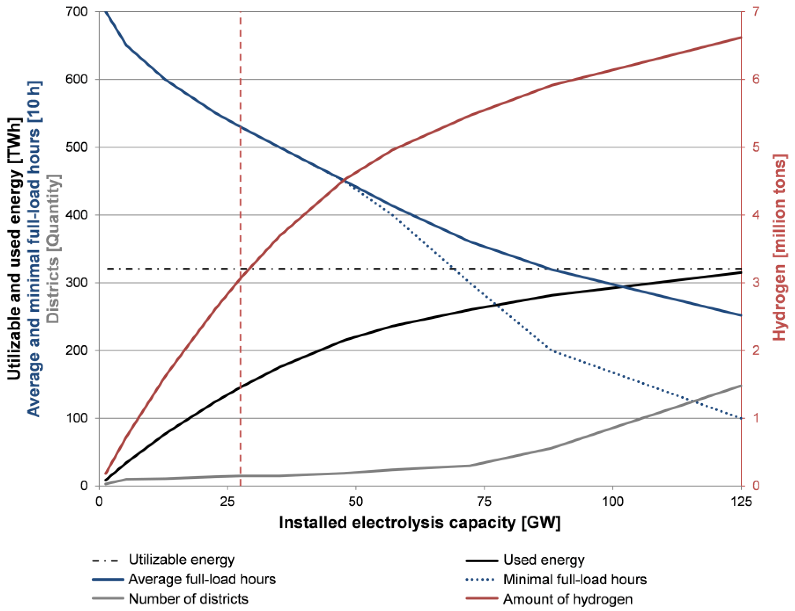
3.2. Utilization of the Surplus by Electrolysis

Subsequent to Section 3.1, in which electricity surpluses are located and quantified, this section determines the possible installable capacity of electrolysis on the district level. For this purpose, two METIS packages are generated: the first installs electrolysers in predefined intervals in each of the 402 districts and ascertains the average number of the electrolysers’ full-load hours based on the residual load on the district level. The second model allows the definition of the minimal and average numbers, respectively, of full-load hours that result in the installed capacity of electrolysis on the district level. Figure 13 depicts the usable, as well as the used, amount of energy, the minimal and average amount of full-load hours, the number of considered districts and the amount of hydrogen produced as the results of iteratively entering different minimal amounts of full-load hours in the second model. The following base causality can be derived from the graphic’s analysis: In the case of increasing the installed capacity of electrolysis, the average number of full-load hours decreases from 7000 at 1 GW to 2520 at 125 GW. Whereas, in the range of up to approximately 50 GW, the average number of full-load hours equals the minimal number, at a capacity level of 125 GW, the difference between average and minimal full-load hours adds up to 1270 h. As a result of an increasing level of electrolysis capacity, the ratio of used to usable energy increases, for instance, from 3% at 1 GW to 98% at 125 GW. On the assumption of a prospective electrolysis efficiency coefficient of 70 %LHV, 6.6 million tons of hydrogen can be produced at an installed electrolysis capacity of 125 GW. It is worth mentioning that two main drawbacks reduce potential hydrogen production. Firstly, taking the economic factors into consideration, electrolysis with 1270 h ends up with hydrogen production costs that are not cost competitive unless negative electricity prices are considered. Secondly, the surplus is only used in the model for the production of hydrogen. Different SC applications like power-to-heat or power-to-chemicals would reduce the potential surplus for hydrogen production. Nevertheless the underlying assumptions show the potential of SC.
In order to fulfil the peak demand of hydrogen from Section 2.2.1, totalling 2.93 million tons in 2052, an electrolysis capacity of 28 GW must be installed in 15 districts, as depicted in Figure 14. In this way, 3064 million tons of hydrogen is produced—approximately 4.4% more than demanded. This overproduction considers hydrogen diffusion in pipelines, compressors or electrolysers, as well as the cushion gas in salt caverns. For the purpose of benchmarking, Feck [68] gives a range of irreversibility from 1.9% to 9.2% for the whole process chain, including production, conditioning, transport, storage and the use of hydrogen.
54% of the energy is curtailed at the selected installed capacity of 28 GW, leading to an average and minimal number of full-load hours of 5300. It becomes apparent that the modelled energy concept provides enough surplus electricity to supply 75% of German road traffic. Moreover, the considerable amount of potential hydrogen of approximately 6.6 million tons allows for a large number of further applications besides the transport sector, such as ammonia and methanol production, in the chemical industry.

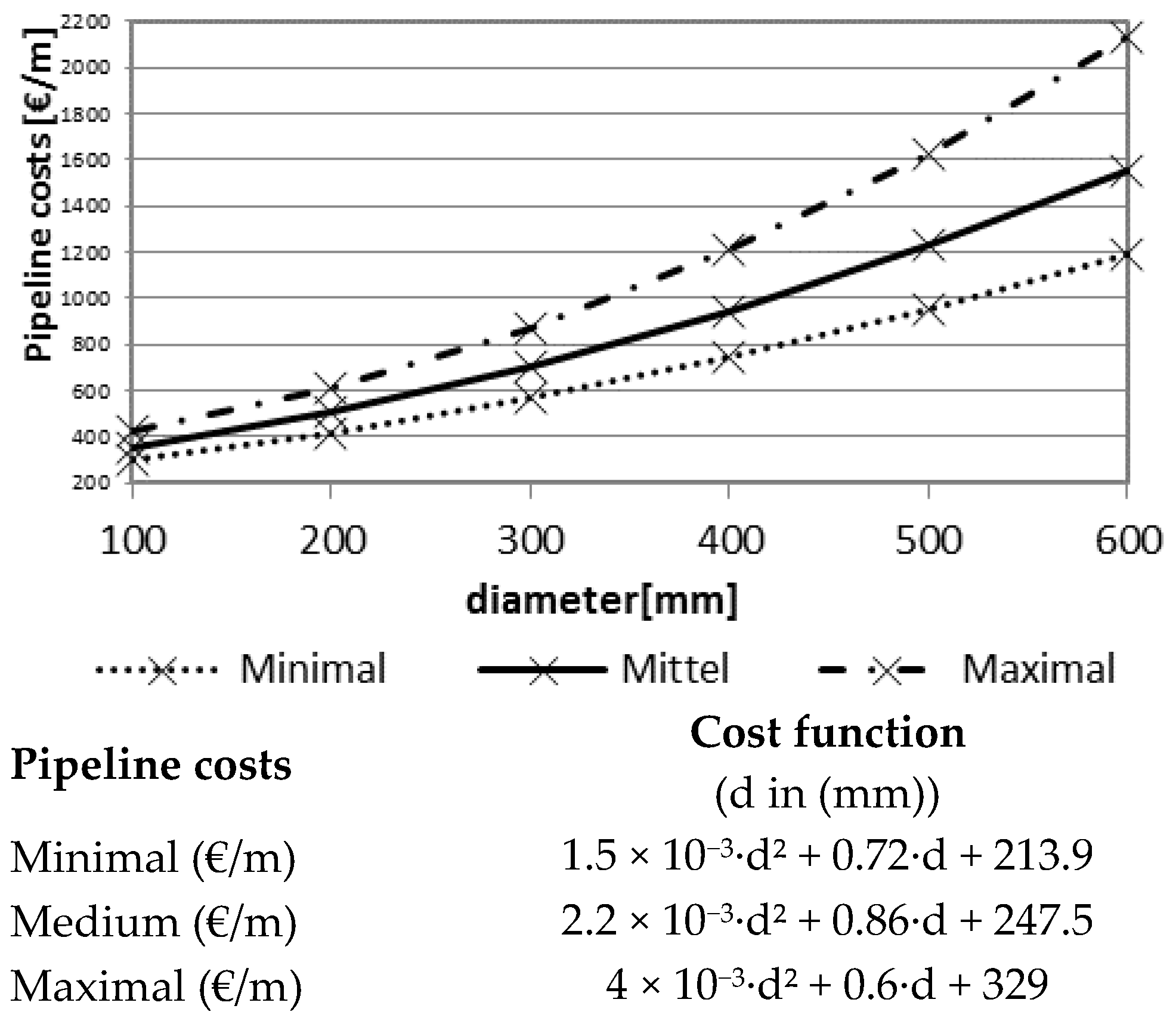
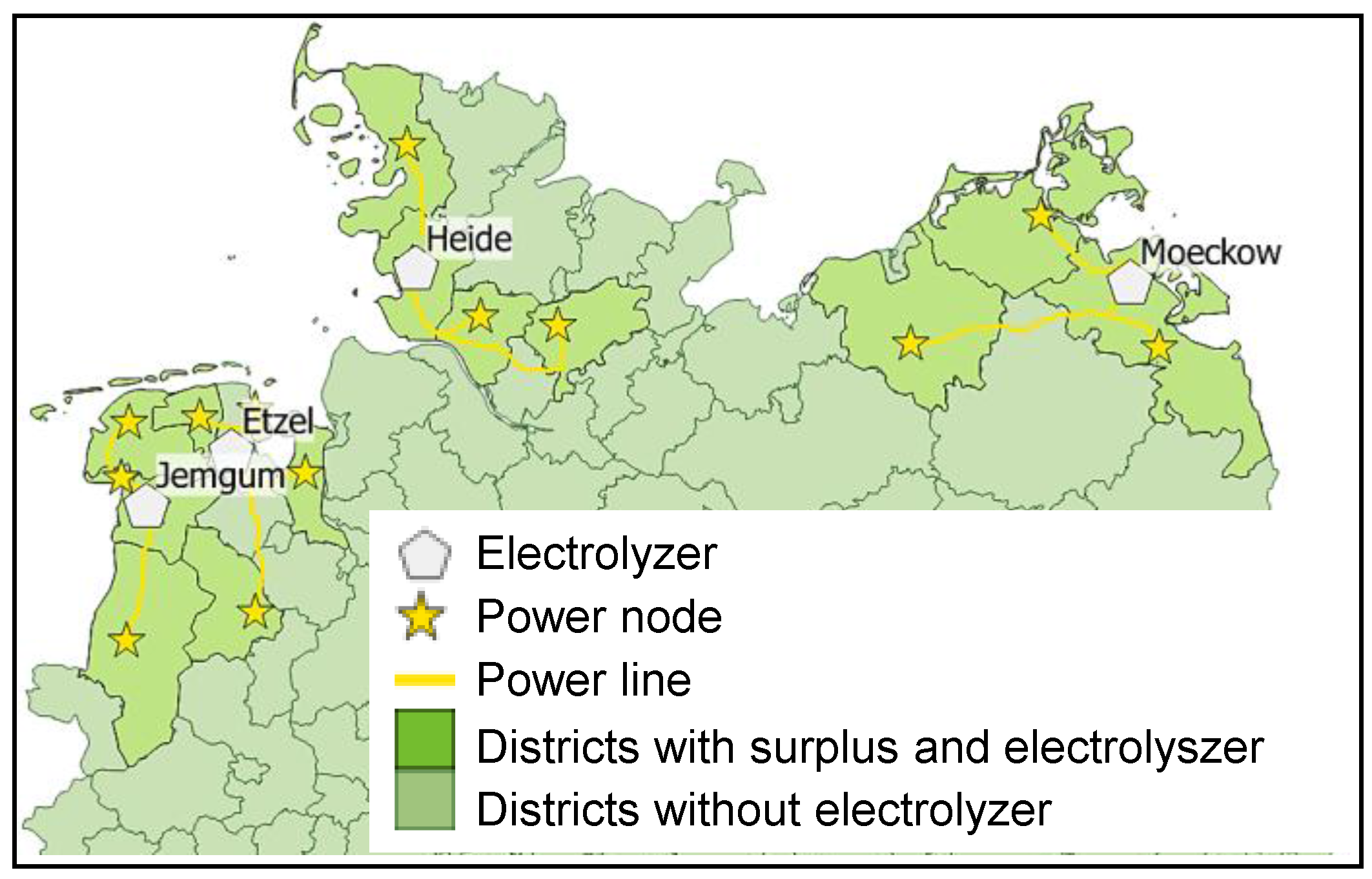
3.3. Hydrogen Pipeline Grid

Because of the wide range of possible energy sources, the plethora of size and locations of production plants, as well as the variety of assumptions regarding hydrogen demand, the future hydrogen supply chain (HSC) appears to be very complex. Most of the infrastructure studies in the literature consider hydrogen demand to be exogenously given, usually based on assumptions on numbers of hydrogen-fuelled vehicles and mileage. Hydrogen production depends on techno-economic assumptions about plants, energy prices and emission restrictions. With regard to a minimal hydrogen infrastructure in early markets, a cost-effective option might be decentralized production.
When it comes to the methodological approach in this paper, the authors assume a high penetration of hydrogen-fuelled vehicles for Germany in 2050 (see Section 2.2.1) and large amounts of gaseous hydrogen to be transported from the production plants (see Section 3.2) to selected filling stations. Fuelling stations must be available all over the country to accommodate the high penetration of hydrogen-fuelled vehicles. The required filling station network is based on the existing network so as to avoid forcing end-consumers to change their habits and use strategically useful locations. With regard to the long-distance infrastructure in Germany, there are few corridors available to develop new routes for pipelines. Thus, the model essentially permits any route to be taken for the transmission pipelines, but prefers paths along the existing high-pressure natural gas grid (see Section 2.2.2).
The hydrogen infrastructure can be divided into a transmission and distribution network, which differ with respect to size, capacity and density. Thus, they are considered separately in the model. The transmission network consists of point-shaped hydrogen sources and sinks, as well as line-shaped connections between them. Preferably, connections between sources and sinks should run alongside each other. While sources can be connected to preferred routes only, sinks can also be connected to each other. By means of a defined cost function, the most cost-efficient route is selected, sinks are sorted according to their ascending distance to the next source and calculated routes become a constraint for the following calculations. The distribution network exhibits the same structure as the transmission network, but is divided into independent district networks. The number of refuelling stations is defined by the respective districts’ hydrogen demand. Pipeline costs are assumed to be dependent on total length and capacity (see Section 2.2.2).
Figure 15 shows the dedicated hydrogen pipeline grid for supplying 2.9 million tons of hydrogen from 28 GW installed electrolysis to 9968 hydrogen fuelling stations. Depending on the respective scenarios, the transmission network costs vary between 5.4 and 8.3 billion €2015, while the pipeline length is 12,104 km. When it comes to the distribution network, the costs vary between 10.2 and 14.7 billion €2015 and the length to connect the 9968 hydrogen fuelling stations is 29,671 km. As expected, the overall distribution network is more expensive than the transmission network. As a comparison, the length of the German natural gas pipeline grid is 470,433 km on the distribution level and 37,695 km on the transmission level [69]. With planned costs in the natural gas pipeline grid of 1010 €/m (DN400 and DN70) [70], investment costs for the transmission grid are assumed to be roughly 38 billion €. This already shows on a scale of comparison between hydrogen or natural gas pipeline grids that the length and costs are not prohibitive in terms of applying this scenario to reality. To ensure feasibility on a more profound level, a detailed economic assessment will be performed in Section 3.4.
To align the study, the methodology used in this paper considers the existing natural gas network as the preferred route for the future hydrogen transmission network, although other routes could also be envisaged. Furthermore, the model does not consider the time variability of either production or demand. Consequently, buffer storages are—implicitly—required.

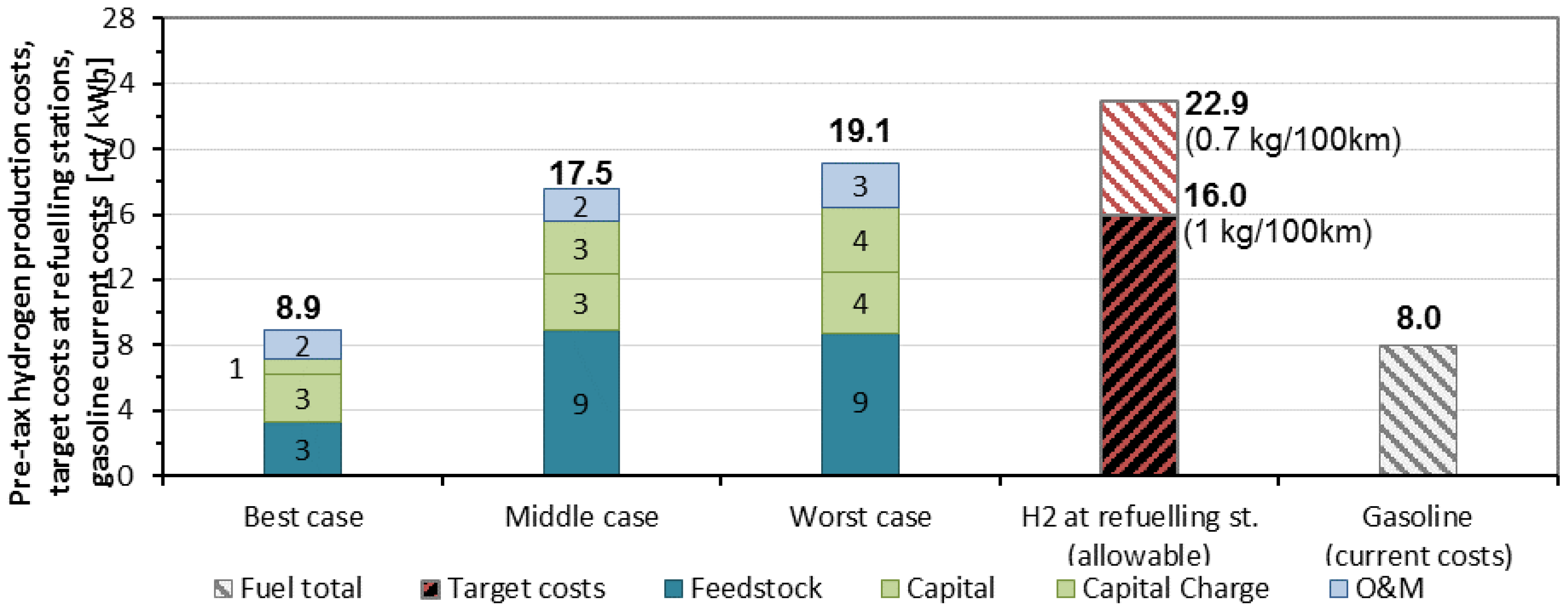
3.4. Economic Assessment

This section describes the calculation of hydrogen production costs down to the filling station. For this purpose, the computed hydrogen pipeline from Section 3.3, which is designed for a peak hydrogen demand of 2.93 million tons in the year 2052 from Section 2.2.1 and for the 15 sources from Section 3.2, is assumed. Within this scope, the methodology outlined by Stolten et al. [20,28,71] is of utility. Thereby, the necessary input values are divided into three categories, namely: “Best case”, “middle case” and “worst case.” The input values of the “best case” match the minimum values from Table 2, whereas the efficiency coefficient closely matches the maximum value. The input values of the “middle case” equate to the mode values from Table 2. Meanwhile, the input values of the “worst case” equate to the mode values from Table 2. The unaltered cost data of the hydrogen pipeline for the transmission grid are adopted from the range of the pipeline costs from Section 3.3. The requirement of 27 TWh storage results from the projected hydrogen consumption of 5.4 million tons [20]. The costs of storage in salt caverns are estimated to amount to 5 billion €. Given a 60-day back-up, the storage requirement augments to 90 TWh, which results in costs of 15 billion € [20]. The same ratio and a hydrogen consumption of 2.9 million tons results in a seasonal storage requirement of 15 TWh and costs of about 2.7 billion €, while an additional 60 day back-up results in a storage requirement of about 48 TWh and costs of about 8 billion €, respectively. The storage costs are considered as follows:
  • Best case: Seasonal storage of 2.9 million tons of hydrogen at a cost of 2.7 billion €.
  • Middle case: Storage of 2.9 million tons of hydrogen for 60 days at a cost of 8 billion €.
  • Worst case: Storage of 5.4 million tons of hydrogen for 60 days at a cost of 15 billion €.
The costs of filling stations for all three cases are estimated at 2 million € per filling station according to Schiebahn et al. [20], noting the few available literature sources in this particular field. Daimler assumes costs of 1 million € per filling station [72]. Geitmann (2004 and 2012) ([73,74]) assumes costs in the range of 0.5 to 1.5 million € depending on size. The National Renewable Energy Lab (2013) [75] reckons costs of about 2.4 million € for the USA. Therefore, 2 million € per filling station appears to be a conservative estimation. Table 2 summarizes the input values of the three cases, “best”, “middle” and “worst.” The efficiency and costs of the electrolysis are validated by the Department of Energy [76].
Figure 16 shows the results of the pre-tax hydrogen cost analysis. The target costs of hydrogen at a filling station can be calculated as follows: Given the pre-tax price of gasoline of 0.08 € per kWh at a filling station and a FCV’s hydrogen consumption of 1 kg per 100 km, target costs would be 16 ct per kWh. These target costs augment to 22.9 ct per kWh for a FCV with a hydrogen consumption of 0.7 kg per 100 km. Hence, these target costs form the benchmark for the hydrogen infrastructure.
Resulting in 8.9, 17.5 and 19.1 ct per kWh, the costs of the “best”, “middle” and “worst case” are below the target costs of FCVs with a consumption of 0.7 kg per 100 km. Within the “best case”, the pre-tax hydrogen costs are even below the target costs of FCVs with a consumption of 1 kg per 100 km.

4. Summary and Conclusions

In proposing a methodology to model SC in terms of linking the power and transport sectors, the “METIS” packages for the power and transport sector has been described in detail (see Section 2). These packages allow the detailed modelling of these sectors in Germany through the year 2050. With this description, the authors intend to supply the scientific community with an approach to conducting comparable SC studies. To show the possibilities of such an approach, a detailed analysis for Germany has been conducted. Therefore, a general scenario that assumes a high share of RES and FCVs has been developed. Furthermore, the surplus in this scenario will be used by electrolysis to produce hydrogen for FCVs. To supply FCVs with this hydrogen, a dedicated hydrogen transmission and distribution pipeline is considered. After describing the sub-packages in “METIS” in more detail, the results in terms of surplus, utilization by electrolysis, hydrogen pipeline grid and economics have been considered to show the possibilities of such an SC modelling approach (see Section 3).
In summary, the results analysis demonstrates the importance of the spatial resolution of the model for a surplus analysis. Because RES are highly spatially distributed, the surplus differs highly depending on the accuracy of the model. The results for Germany showed that considering the installed capacities of the RES in the scenario, even with the physically impossible consideration of a “copper plate” and no storage losses or limitations, a surplus of 165 TWh will be produced and therefore a possibility of power-to-X applications is apparent (see Section 3.1). In order to fulfil the peak demand of hydrogen of 2.93 million tons in the year 2052, an electrolysis capacity of 28 GW in 15 districts in Germany must be achieved. Without considering minimal full load hours of the electrolysis, there is even a possibility of producing 6.6 million tons of hydrogen in Germany (see Section 3.2). Depending on the respective scenarios, the transmission network’s—to connect the 28 GW of electrolysis capacity to the hubs—costs vary between 5.4 and 8.3 billion € (2015), while the pipeline length is 12,104 km. When it comes to the distribution network—to connect the hubs with the 9968 total hydrogen fuelling stations—the costs vary between 10.2 and 14.7 billion € (2015) and the pipeline length is 29,671 km (see Section 3.3). A pre-tax hydrogen cost analysis showed that the resulting costs of a “best”, “middle” and “worst case” scenario with 8.9, 16.5 and 19.1 ct per kWh are below the target costs of FCVs with a consumption of 0.7 kg per 100 km. Within the “best case”, the pre-tax hydrogen costs are even below the target costs of FCVs with a consumption of 1 kg per 100 km (see Section 3.4).
This paper not only showed a detailed approach to modelling SC in terms of linking the power and transport sectors, but also the economic possibility of installing a dedicated hydrogen pipeline grid for Germany.

Acknowledgments

This work was supported by the Helmholtz Association under the Joint Initiative “EnergySystem 2050—A Contribution of the Research Field Energy.” Furthermore, it was supported by funding of the Virtual Institute for Power to Gas and Heat by the Ministry of Innovation, Science and Research of North Rhine-Westphalia. The authors would like to thank the numerous master and bachelor students who contributed to the METIS packages and Christopher Wood for editing this paper.

Author Contributions

Martin Robinius proposed the research topic and the structure of the paper. He developed with his master students all the models and analysed all results as part of his Ph.D. Thesis. Alexander Otto, Konstantinos Syrandis, David S. Ryberg, Philipp Heuser and Lara Welder wrote the paper (ranked by their contribution). Thomas Grube, Peter Markewitz and Vanessa Tietze took part in revising the paper. Detlef Stolten proposed the research topic and took part in validating the idea and revising the paper.

Conflicts of Interest

The authors declare no conflict of interest.

References

  1. Robinius, M.; Otto, A.; Heuser, P.; Welder, L.; Syranidis, K.; Ryberg, D.S.; Grube, T.; Markewitz, P.; Peters, R.; Stolten, D. Linking the power and transport sectors—Part 1: The principle of sector coupling. Energies 2017, 10, 956. [Google Scholar]
  2. Markewitz, P.; Kuckshinrichs, W.; Martinsen, D.; Hake, J.F. IKARUS—A fundamental concept for national GHG-mitigation strategies. Energy Convers. Manag. 1996, 37, 777–782. [Google Scholar] [CrossRef]
  3. Fraunhofer ISE. 100% Erneuerbare Energien für Strom und Wärme in Deutschland. 2012. Available online: http://www.ise.fraunhofer.de/de/veroeffentlichungen/veroeffentlichungen-pdf-dateien/studien-und-konzeptpapiere/studie-100-erneuerbare-energien-in-deutschland.pdf (accessed on 20 February 2017). (In German).
  4. Fraunhofer IWES. Geschäftsmodell Energiewende. Eine Antwort auf das “Die-Kosten-der-Energiewende”-Argument; IWES: Kassel Germany, 2014. (In German) [Google Scholar]
  5. Lunz, B.; Stöcker, P.; Eckstein, S.; Nebel, A.; Samadi, S.; Erlach, B.; Fischedick, M.; Elsner, P.; Sauer, D.U. Scenario-based comparative assessment of potential future electricity systems—A new methodological approach using Germany in 2050 as an example. Appl. Energy 2016, 171, 555–580. [Google Scholar] [CrossRef]
  6. Pfenninger, S.; Hawkes, A.; Keirstead, J. Energy systems modeling for twenty-first century energy challenges. Renew. Sustain. Energy Rev. 2014, 33, 74–86. [Google Scholar] [CrossRef]
  7. Guandalini, G.; Robinius, M.; Grube, T.; Campanari, S.; Stolten, D. Long-term power-to-gas potential from wind and solar power: A country analysis for Italy. Int. J. Hydrogen Energy 2017, 42, 13389–13406. [Google Scholar] [CrossRef]
  8. Varone, A.; Ferrari, M. Power to liquid and power to gas: An option for the German Energiewende. Renew. Sustain. Energy Rev. 2015, 45, 207–218. [Google Scholar] [CrossRef]
  9. Schemme, S.; Samsun, R.C.; Peters, R.; Stolten, D. Power-to-fuel as a key to sustainable transport systems—An analysis of diesel fuels produced from CO2 and renewable electricity. Fuel 2017, 205, 198–221. [Google Scholar] [CrossRef]
  10. Otto, A.; Robinius, M.; Grube, T.; Schiebahn, S.; Praktiknjo, A.; Stolten, D. Power-to-Steel: Reducing CO2 through the Integration of Renewable Energy and Hydrogen into the German Steel Industry. Energies 2017, 10, 451. [Google Scholar] [CrossRef]
  11. Nastasi, B.; Basso, G.L. Hydrogen to link heat and electricity in the transition towards future Smart Energy Systems. Energy 2016, 110, 5–22. [Google Scholar] [CrossRef]
  12. Grueger, F.; Möhrke, F.; Robinius, M.; Stolten, D. Early power to gas applications: Reducing wind farm forecast errors and providing secondary control reserve. Appl. Energy 2017, 192, 551–562. [Google Scholar] [CrossRef]
  13. Guandalini, G.; Campanari, S.; Romano, M.C. Power-to-gas plants and gas turbines for improved wind energy dispatchability: Energy and economic assessment. Appl. Energy 2015, 147, 117–130. [Google Scholar] [CrossRef]
  14. De Santoli, L.; Basso, G.L.; Bruschi, D. A small scale H2NG production plant in Italy: Techno-economic feasibility analysis and costs associated with carbon avoidance. Int. J. Hydrogen Energy 2014, 39, 6497–6517. [Google Scholar] [CrossRef]
  15. Basso, G.L.; Nastasi, B.; Garcia, D.A.; Cumo, F. How to handle the Hydrogen enriched Natural Gas blends in combustion efficiency measurement procedure of conventional and condensing boilers. Energy 2017, 123, 615–636. [Google Scholar] [CrossRef]
  16. Robinius, M. Strom- und Gasmarktdesign zur Versorgung des Deutschen Straßenverkehrs mit Wasserstoff. Ph.D. Thesis, RWTH Aachen University, Aachen, Germany, 2015. (In German). [Google Scholar]
  17. Robinius, M.; Stolten, D. Power-to-Gas: Quantifizierung lokaler Stromüberschüsse in Deutschland anhand unterschiedlicher Windenergie-Ausbaustufen. In Proceedings of the 9th Internationale Energiewirtschaftstagung, Wien, Austria, 20 February 2015. (In German). [Google Scholar]
  18. Ter Stein, F. Lokal und Temporär Aufgelöstes Strompreismodell in Deutschland. Master’s Thesis, RWTH-Aachen, Aachen, Germany, 2015. (In German). [Google Scholar]
  19. Terjung, L. Residuallastmodellierung zur Analyse eines Zonalen Strommarktmodells bei hohen Anteilen Erneuerbarer Energien. Bachelor’s Thesis, RWTH-Aachen, Aachen, Germany, 2015. (In German). [Google Scholar]
  20. Schiebahn, S.; Grube, T.; Robinius, M.; Tietze, V.; Kumar, B.; Stolten, D. Power to gas: Technological overview, systems analysis and economic assessment for a case study in Germany. Int. J. Hydrogen Energy 2015, 40, 4285–4294. [Google Scholar] [CrossRef]
  21. Tarrés, H.C. Determination of Potential Locations for Wind Turbines in Germany with Geospatial Information Systems. Bachelor’s Thesis, RWTH-Aachen, Aachen, Germany, 2014. [Google Scholar]
  22. Robinius, M.; ter Stein, F.; Schiebahn, S.; Stolten, D. Lastmodellierung und -visualisierung mittels Geoinformationssystemen. In Proceedings of the 13rd Symposium Energieinnovation, Graz, Austria, 12–14 February 2014. (In German). [Google Scholar]
  23. Robinius, M.; Rodriguez, R.A.; Kumar, B.; Andresen, G.B.; ter Stein, F.; Schiebahn, S.; Stolten, D. Optimal placement of electrolysers in a German power-to-gas infrastructure. In Proceedings of the 20th World Hydrogen Energy Conference (WHEC 2014), Gwangju, Korea, 15–20 June 2014. [Google Scholar]
  24. Franco, C.S.M. Estimation of the Technical Photovotaic Potential in Germany Using Geospatial Information System; RWTH-Aachen: Aachen, Germany, 2014. [Google Scholar]
  25. Tietze, V.; Stolten, D. Comparison of hydrogen and methane storage by means of a thermodynamic analysis. Int. J. Hydrogen Energy 2015, 40, 11530–11537. [Google Scholar] [CrossRef]
  26. Baufumé, S.; Grüger, F.; Grube, T.; Krieg, D.; Linssen, J.; Weber, M.; Hake, J.F.; Stolten, D. GIS-based scenario calculations for a nationwide German hydrogen pipeline infrastructure. Int. J. Hydrogen Energy 2013, 38, 3813–3829. [Google Scholar] [CrossRef]
  27. Robinius, M.; Stein, F.T.; Schwane, A.; Stolten, D. A Top-Down Spatially Resolved Electrical Load Model. Energies 2017, 10, 361. [Google Scholar] [CrossRef]
  28. Schiebahn, S.; Grube, T.; Robinius, M.; Otto, A.; Kumar, B.; Weber, M.; Stolten, D. Power to Gas. In Transition to Renewable Energy Systems; Stolten, D., Scherer, V., Eds.; Wiley-VCH: Hoboken, NJ, USA, 2013; pp. 813–849. [Google Scholar]
  29. Krieg, D. Konzept und Kosten eines Pipelinesystems zur Versorgung des deutschen Straßenverkehrs mit Wasserstoff. Ph.D. Thesis, Forschungszentrums Jülich, Jülich, Germany, 2012. (In German). [Google Scholar]
  30. ENTSO-E, Consumption Data. 2013. Available online: https://www.entsoe.eu/data/data-portal/consumption/ (accessed on 20 February 2017).
  31. Ter Stein, F. Regionale elektrische Lastmodellierung mittels Datenbank- und Geoinformationssystemen. Master’s Thesis, RWTH-Aachen, Aachen, Germany, 2014. (In German). [Google Scholar]
  32. Übertragungsnetzbetreiber. Netzentwicklungsplan Strom 2025 Offshore-Netzentwicklungsplan 2025 Version 2015; 2. Entwurf. 2016. Available online: https://www.netzentwicklungsplan.de/sites/default/files/paragraphs-files/NEP_ONEP_2025_2_Entwurf_Zahlen_Daten_Fakten.pdf (accessed on 20 February 2017). (In German).
  33. European Environment Agency. Corine Landcover 2006. Available online: https://www.eea.europa.eu/publications/COR0-landcover (accessed on 20 February 2017).
  34. European Topic Centre on Biological Diversity. EUNIS-sites: Common Database on Designated Areas. 2015. Available online: http://bd.eionet.europa.eu/activities/products/cdda (accessed on 20 February 2017).
  35. Geofabrik. Open Street Map. Available online: http://download.geofabrik.de/europe/germany.html (accessed on 20 February 2017).
  36. Adaramola, M.S.; Krogstad, P.Å. Experimental investigation of wake effects on wind turbine performance. Renew. Energy 2011, 36, 2078–2086. [Google Scholar] [CrossRef]
  37. Deutscher Wetterdienst. Winddaten für Deutschland. 2014. Available online: http://www.dwd.de/bvbw/appmanager/bvbw/dwdwwwDesktop?_nfpb=true&_pageLabel=_dwdwww_klima_umwelt_klimadaten_deutschland&_state=maximized&_windowLabel=T82002&T82002gsbDocumentPath=Navigation%252FOeffentlichkeit%252FKlima__Umwelt%252FKlimadaten%252Fkldaten__kostenfrei%252Fkldat__D__gebiete__wind__node.html%253F__nnn%253Dtrue (accessed on 20 February 2017). (In German).
  38. AG Energiebilanzen. Zeitreihen zur Entwicklung der erneuerbaren Energien in Deutschland; AG Energiebilanzen: Berlin, Germany, 2014. [Google Scholar]
  39. EnergyMap. Die Daten der EnergyMap zum Download. 2014. Available online: http://www.energymap.info/download.html (accessed on 20 February 2017).
  40. Quaschning, V. Systemtechnik einer klimaverträglichen Elektrizitätsversorgung in Deutschland für das 21. Jahrhundert; VDI-Verlag: Düsseldorf, Germany, 2000. (In German) [Google Scholar]
  41. Fraunhofer, I.W.E.S. Vorstudie zur Integration großer Anteile Photovoltaik in Die Elektrische Energieversorgung; IWES: Kassel, Germany, 2011. (In German) [Google Scholar]
  42. Lödl, M.; Kerber, G.; Witzmann, R.; Hoffmann, C.; Metzger, M. Abschätzung des Photovoltaik-Potenzials auf Dachflächen in Deutschland. In Proceedings of the Symposium Energieinnovation, Graz, Austria, 10–12 February 2010. (In German). [Google Scholar]
  43. Wesselak, V. Regenerative Energietechnik; Springer: Berlin/Heidelberg, Germany, 2013. (In German) [Google Scholar]
  44. Agora Energiewende. Agorameter-Dokumentation. 2014. Available online: http://www.agora-energiewende.de/fileadmin/downloads/sonstiges/Hintergrunddokumentation_Agora-Meter.pdf (accessed on 20 February 2017). (In German).
  45. Arbeitsgemeinschaft Energiebilanzen e.V. Energieverbrauch in Deutschland im Jahr 2013. Available online: www.ag-energiebilanzen.de/index.php?article_id=29&fileName=ageb_jahresbericht2013_20140317.pdf (accessed on 20 February 2017). (In German).
  46. Bundesnetzagentur. Kraftwerksliste 2013; Bundesnetzagentur: Bonn, Germany, 2013. [Google Scholar]
  47. Wend, A. Modellierung des Deutschen Strommarktes unter Verwendung der Residuallast; Institut für Brennstoffzellen, RWTH Aachen: Aachen, Germany, 2014. (In German) [Google Scholar]
  48. 50 Hertz Transmission GmbH. Lastflüsse. 2013. Available online: http://www.50hertz.com/de/Anschluss-Zugang/Engpassmanagement/Lastfluesse (accessed on 20 February 2017).
  49. Amprion GmbH. Berechnung von Regelblocküberschreitenden Übertragungskapazitäten zu Internationalen Partnernetzen; Amprion GmbH: Dortmund, Germany, 2012; p. 8. (In German) [Google Scholar]
  50. Amprion GmbH. Grenzüberschreitende Lastflüsse; Amprion GmbH: Dortmund, Germany, 2013. [Google Scholar]
  51. ENTSO-E. Exchange Data. 2014. Available online: https://www.entsoe.eu/data/data-portal/exchange/Pages/default.aspx (accessed on 20 February 2017).
  52. Nord Pool Spot. Historical Market Data. 2015. Available online: http://www.nordpoolspot.com/historical-market-data/ (accessed on 20 February 2017).
  53. Tennet TSO GmbH. Grenzüberschreitende Lastflüsse/abgestimmte Fahrpläne. 2015. Available online: https://www.tennettso.de/site/Transparenz/veroeffentlichungen/netzkennzahlen/grenzueberschreitende-lastfluesse (accessed on 20 February 2017). (In German).
  54. TransnetBW GmbH. Grenzüberschreitende Lastflüsse. 2015. Available online: http://www.transnetbw.de/de/kennzahlen/lastdaten/grenzueberschreitende-lastfluesse?app=last&activeTab=table&auswahl=day&date=10.03.2015&view=3&selectMonatDownload=15 (accessed on 20 February 2017). (In German).
  55. Übertragungsnetzbetreiber. Netzentwicklungsplan Strom 2014 zweiter Entwurf der Übertragungsnetzbetreiber; Übertragungsnetzbetreiber: Bonn, Germany, 2014; p. 137. (In German) [Google Scholar]
  56. Bystry, T. H2 mobility—Germany. In Proceedings of the H2Expo 2014, Hamburg, Germany, 23–26 September 2014. [Google Scholar]
  57. De Colvenaer, B. Fuel Cells and Hydrogen Joint Undertaking European Hydrogen Infrastructure Activities. In Proceedings of the H2Expo 2014, Hamburg, Germany, 23–26 September 2014. [Google Scholar]
  58. Ehret, O. Nationale initiativen für wasserstoff als marktnahe querschnittstechnologie; DBI-Fachforum ENERGIESPEICHER—HYBRIDNETZE: Berlin, Germany, 2012. (In German) [Google Scholar]
  59. GermanHy. Woher kommt der Wasserstoff in Deutschland bis 2050? GermanHy: Berlin, Germany, 2009. (In German) [Google Scholar]
  60. Höft, U. Lebenszykluskonzepte: Grundlage für das Strategische Marketing-und Technologiemanagement; Erich Schmidt Verlag GmbH & Co. KG: Berlin, Germany, 1992. (In German) [Google Scholar]
  61. Bundesministerium für Verkehr und digitale Infrastruktur. Verkehr in Zahlen 2014/2015; Bundesministerium für Verkehr und digitale Infrastruktur: Berlin, Germany, 2015. (In German) [Google Scholar]
  62. Fraunhofer ISI. Markthochlaufszenarien für Elektrofahrzeuge—Langfassung; Fraunhofer ISI: Karlsruhe, Germany, 2014. [Google Scholar]
  63. Kraftfahrt-Bundesamt. Kraftfahrzeugbestand nach Kraftfahrzeugarten; Kraftfahrt-Bundesamt: Flensburg, Germany, 2015. (In German) [Google Scholar]
  64. Toyota. Serien-Brennstoffzellenfahrzeug—Beste Effizienz am Markt. 2015. Available online: http://www.toyota.de/news/details-2015–43.json (accessed on 20 February 2017). (In German).
  65. Keles, D.; Wietschel, M.; Möst, D.; Rentz, O. Market penetration of fuel cell vehicles—Analysis based on agent behaviour. Int. J. Hydrogen Energy 2008, 33, 4444–4455. [Google Scholar] [CrossRef]
  66. Reuß, M.; Grube, T.; Robinius, M.; Preuster, P.; Wasserscheid, P.; Stolten, D. Seasonal storage and alternative carriers: A flexible hydrogen supply chain model. Appl. Energy 2017, 200, 290–302. [Google Scholar] [CrossRef]
  67. Grüger, F. Nachfrageorientierte Kapazitätsbestimmung einer Wasserstoffinfrastruktur für Deutschland. Master’s Thesis, RWTH Aachen, Aachen, Germany, 2011. (In German). [Google Scholar]
  68. Feck, T. Wasserstoff-Emissionen und ihre Auswirkungen auf den Arktischen Ozonverlust: Risikoanalyse einer globalen Wasserstoffwirtschaft; Forschungszentrum Jülich: Jülich, Germany, 2009. (In German) [Google Scholar]
  69. Bundesnetzagentur and Bundeskartellamt. Monitoringbericht 2013, 3. Auflage; Bundesnetzagentur and Bundeskartellamt: Bonn, Germany, 2014. (In German) [Google Scholar]
  70. Die Fernleitungsnetzbetreiber. Netzentwicklungsplan Gas 2015—Konsultationsdokument; Die Fernleitungsnetzbetreiber: Bonn, Germany, 2015. (In German) [Google Scholar]
  71. Stolten, D.; Grube, T.; Mergel, J. Beitrag Elektrochemischer Energietechnik zur Energiewende; VDI-Berichte: Düsseldorf, Germany, 2012. (In German) [Google Scholar]
  72. Südwest Presse. Daimler baut früher Autos mit Brennstoffzellen. 2011. Available online: http://www.swp.de/ulm/nachrichten/wirtschaft/Daimler-baut-frueher-Autos-mit-Brennstoffzellen;art4325,988215 (accessed on 20 February 2017). (In German).
  73. Geitmann, S. Wasserstoff und Brennstoffzellen: Die Technik von Morgen; Hydrogeit-Verlag: Oberkrämer, Germany, 2004. (In German) [Google Scholar]
  74. Geitmann, S. Energiewende 3.0: Mit Wasserstoff und Brennstoffzellen; Hydrogeit-Verlag: Oberkrämer, Germany, 2012. (In German) [Google Scholar]
  75. National Renewable Energy Lab. Hydrogen Station Cost Estimates—Comparing Hydrogen Station Cost Calculator Results with Other Recent Estimates; National Renewable Energy Lab: Golden, CO, USA, 2013.
  76. DOE Hydrogen and Fuel Cells Program Record. Hydrogen Production Cost from PEM Electrolysis; U.S. Department of Energy: Washington, DC, USA, 2014.
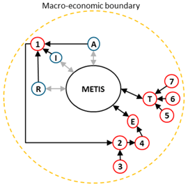
Figure 1. Different modelling approaches for sector coupling (SC) analyses, comprising: a closed model environment (a); and open model environment (b).
Energies 10 00957 g001
Figure 2. Example of the installed capacity, produced electricity and average full load hours by the year 2050 in Germany.
Energies 10 00957 g002
Figure 3. Results of land eligibility investigation of Germany. Sites that are suitable for wind turbine are shown in brown (113,126 km2), while areas that are inaccessible due to poor land cover, protected regions, or being too close to roads and buildings are shown in white (244,043 km2).
Energies 10 00957 g003
Figure 4. Installed PV capacity on municipalities level in Germany by 2014 (Input Data from EnergyMap [39]), totalling 39.4 GW (left); and installed PV capacity on the municipalities level by 2050, which totals 55 GW (right).
Energies 10 00957 g004
Figure 5. Result of the residual load analysis before grid dynamics are included at the municipality level. Blue indicates regions with a negative residual load, meaning that they have excess energy to lend. These regions are most heavily clustered in the north of Germany, where wind potential is greatest. Red indicates regions with a positive residual load.
Energies 10 00957 g005
Figure 6. Location and installed capacities of conventional power plants in Germany (a); and transmission lines at 380 and 220 kV, in addition to high voltage direct current transmission (b). Data according to: Bundesnetzagetur (2013) [46] (a); and Übertragungsnetzbetreiber (2016) [32] (b).
Energies 10 00957 g006
Figure 7. Number of fuel-cell vehicles in the IEK-3 model, in the Lead scenario and Scenario 3, according to Keles et al. [65] and annual consumption and peak demand for hydrogen.
Energies 10 00957 g007
Figure 8. Hydrogen demand in 402 districts according to the model in 2040 (left); and 2050 with peak demand of hydrogen (right).
Energies 10 00957 g008
Figure 9. Hydrogen cost at the fuelling station regarding the full supply chain (Electrolysis, seasonal storage, transport, fuelling station) [66].
Energies 10 00957 g009
Figure 10. Cost function of pipeline costs, including material and compression depending on diameter [29].
Energies 10 00957 g010
Figure 11. Electricity production, electricity demand and residual energy with six different input assumptions.
Energies 10 00957 g011
Figure 12. Result of the residual load analysis: before grid dynamics are included (left); and after grid dynamics are included (right), on the county level. The blue indicates regions with a negative residual load, meaning that they have excess energy to lend. These regions are most heavily clustered in the north of Germany, where wind potential is greatest. Red indicates regions with a positive residual load.
Energies 10 00957 g012
Figure 13. Utilizable and used energy, average and minimal full-load hours, quantity of districts and produced hydrogen, by use of an efficiency coefficient of 70% and increasing electrolysis capacity.
Energies 10 00957 g013
Figure 14. Selected districts to cover the peak-demand of hydrogen of 2.93 million tons in the year 2052.
Energies 10 00957 g014
Figure 15. Dedicated hydrogen pipeline grid to supply 2.9 million tons of hydrogen from 28 GW installed electrolysis to 9968 hydrogen fuelling stations.
Energies 10 00957 g015
Figure 16. Pre-tax cost analysis for the three cases from Table 2.
Energies 10 00957 g016
Table 1. The utilized sub-models of models for energy transformation and integration systems (METIS) for this paper.
Energies 10 00957 i001Sub-ModelsConsidered Sectors
1Electricity-Load-Model (ELM) [16,22,27]TTransport
2Regional Electricity Market Program (REMP) [16]IIndustry, trade and commerce
3RES Potential Model [16,17]RResidential/households
4Electricity Grid Model [16]AAgriculture
5Hydrogen Pipeline Model [20,25,26,28,29]EEnergy
6Hydrogen Demand Model [16]
7Electrolysis Utilization Model [16]
Table 2. Input values of pre-tax hydrogen cost analysis of the updated energy concept from the IEK-3, compare Figure 16.
Input-DataBest CaseMiddle CaseWorst Case
Electricity costs (ct/kWh)2.45.86
Weighted average cost of capital (WACC) (%)388
Electrolysis:
Investment costs (€/kW)446500500
Efficiency (%)767070
Operating costs as a share of the investment costs (%)0.433
Hydrogen Storage (Salt Caverns):
Size (TWh)154890
Costs (Bil. €)2.7815
Hydrogen Pipeline Grid:
Peak hydrogen demand (Mil. t)2.92.92.9
Costs transmission pipeline (Bil. €)5.46.78.3
Costs distribution pipeline (Bil. €)10.11214.6
Hydrogen Fuelling Station:
Costs per fuelling station (Mil. €)222

