Real-Time Distributed Economic Model Predictive Control for Complete Vehicle Energy Management


1
Department of Electrical Engineering, Eindhoven University of Technology, 5612 AZ Eindhoven, The Netherlands
2
DAF Trucks NV, Vehicle Control Group, 5643 TW Eindhoven, The Netherlands
*
Author to whom correspondence should be addressed.
†
All authors contributed equally to this work.
Energies 2017, 10(8), 1096; https://doi.org/10.3390/en10081096
Submission received: 15 June 2017
/
Revised: 19 July 2017
/
Accepted: 20 July 2017
/
Published: 27 July 2017
(This article belongs to the Special Issue Energy Management Control)
Abstract
:In this paper, a real-time distributed economic model predictive control approach for complete vehicle energy management (CVEM) is presented using a receding control horizon in combination with a dual decomposition. The dual decomposition allows the CVEM optimization problem to be solved by solving several smaller optimization problems. The receding horizon control problem is formulated with variable sample intervals, allowing for large prediction horizons with only a limited number of decision variables and constraints in the optimization problem. Furthermore, a novel on/off control concept for the control of the refrigerated semi-trailer, the air supply system and the climate control system is introduced. Simulation results on a low-fidelity vehicle model show that close to optimal fuel reduction performance can be achieved. The fuel reduction for the on/off controlled subsystems strongly depends on the number of switches allowed. By allowing up to 15-times more switches, a fuel reduction of 1.3% can be achieved. The approach is also validated on a high-fidelity vehicle model, for which the road slope is predicted by an e-horizon sensor, leading to a prediction of the propulsion power and engine speed. The prediction algorithm is demonstrated with measured ADASIS information on a public road around Eindhoven, which shows that accurate prediction of the propulsion power and engine speed is feasible when the vehicle follows the most probable path. A fuel reduction of up to 0.63% is achieved for the high-fidelity vehicle model.
1. Introduction
The need for fuel-efficient road transport has largely driven the development of new automotive technology and research over the last decades. A well-known and promising development is the hybrid powertrain that, typically, consists of an internal combustion combined with an electric machine and a high-voltage battery. The electric machine can recover (some of) the brake energy, which is then stored in the high-voltage battery. The stored energy can later be used to provide propulsion power so that the power needed from the internal combustion engine is reduced and the engine can be operated at a more efficient operating point. An energy management strategy is essential to control these energy flows while maximizing the efficiency. However, the energy flows in a vehicle are not limited to the energy flows needed for propulsion. Heavy-duty vehicles in particular tend to have many subsystems on board to support the functionality of the vehicle, which can consume a significant amount of energy, a refrigerated semi-trailer and an air supply system being notorious examples. The optimization of all of these energy flows individually does not automatically guarantee optimal energy efficiency at the vehicle level. Therefore, a holistic system approach is needed, i.e., complete vehicle energy management (CVEM; [1]). The broad range of functionalities for heavy-duty vehicles has led to many different powertrain configurations augmented with different auxiliary subsystems. This requires CVEM to handle the growing complexity with the number of subsystems, while at the same time, it needs to be flexible for the many different configurations that exist for a heavy-duty vehicle. Indeed, developing a new energy management strategy for each vehicle configuration is time consuming and very expensive.
Many different solution strategies for solving the energy management problem have been proposed over the past decades. The proposed solution strategies can be divided into so-called offline and online solution strategies [2,3]. Offline solution strategies have been developed based on, e.g., dynamic programming (DP; see, e.g., [4,5,6]), Pontryagin’s minimum principle (PMP; see, e.g., [7,8,9,10]) or convex optimization (see, e.g., [11,12]). The offline solution strategies require all disturbances to be known (e.g., the driving cycle) so that the global optimal solution can be computed and can therefore not be implemented in real time. Still, they do provide a benchmark for online solution methods and are therefore valuable tools.
Examples of online solution strategies that are real-time implementable are rule-based strategies (see, e.g., [13,14]), equivalent consumption minimization strategies (ECMS; see, e.g., [15,16,17]) and solution strategies based on model predictive control (MPC; see, e.g., [18,19,20]). The MPC strategies are interesting as they naturally take prediction information into account. The prediction information can be stochastic as in [21,22] or deterministic as in [18,19,20,23,24,25]. The future power demand for the deterministic MPC strategies can be predicted as a function of the current power demand, e.g., the power demand is exponentially decaying in [23,24] and held constant in [25]. The future power demand can also be predicted with a vehicle model and road preview information, as in [18], or it can be assumed that the future power demand is exactly known, as in [19,20]. The choice of the cost function also leads to many variations in MPC strategies. The cost function generally weights the fuel consumption, with or without additional terms penalizing the final state, the state deviations and the size of the control inputs, which leads to many penalizing parameters.
While the aforementioned online solution strategies might be able to handle the complexity of the CVEM problem, the flexibility of these strategies is poor. Rule-based strategies require a new set of rules for every subsystem that is added to the CVEM problem; ECMS requires tuning of an equivalence factor for each additional state in the CVEM problem; and MPC requires reformulating the optimal control problem, the cost function and tuning of the penalizing parameters each time a subsystem is added. To enhance the flexibility of vehicle energy management, a distributed offline solution strategy is proposed in [26], and online solutions are proposed in [27,28,29]. In [27], an online game-theoretic approach to CVEM is presented, but prediction information is not taken into account. In [28], an online game-theoretic approach in combination with MPC is presented, which does utilize prediction information, but requires solving a nonlinear program. In [29], flexibility is obtained by using the Alternating Direction Method of Multipliers (ADMM), while ideas based on ECMS are used to provide the equivalent costs at a supervisory level. While each of these solution strategies is interesting and provides a certain degree of flexibility, they require still a significant amount of tuning, while real-time implementability is not guaranteed.
In this paper, we propose to use distributed economic MPC [30,31,32] to solve the CVEM problem. In particular, we define the optimal control problem over a receding horizon and apply a dual decomposition to this optimal control problem, as we proposed in [33], which uses the framework presented in [26]. The application of the dual decomposition results in small-sized linearly-constrained quadratic programs (LCQP) for each of the subsystems, which can be efficiently solved in real time with embedded LCQP solvers. The optimal control problem is then solved at each time instant over a horizon of N samples after which only the decisions at the time instant k are implemented. The conventional cost function in MPC is generally chosen as a quadratic performance index, which is a measure of the predicted deviation of the error between the states and inputs from their corresponding steady-state values, as was done in the context of energy management in, e.g., [23,24,25]. For CVEM, the cost function follows from the desire to minimize the energy losses in the vehicle. Therefore, we will adopt the terminology as in [30], which uses economic MPC, as forcing the system to operate around a pre-specified steady-state value is not necessarily the most efficient.
Choosing the length of the prediction horizon for economic MPC is a delicate decision. On the one hand, the need for soft final state constraints to be added to the cost function, as is done in, e.g., [23], can be avoided by taking a long prediction horizon. On the other hand, the number of decision variables is typically proportional to the length of the prediction horizon, which leads to a preference for short prediction horizons to allow for real-time implementation. Therefore, we will use variable prediction time intervals that allows long prediction horizons with a limited number of decision variables. These were first introduced in [33].
Contrary to [33], in this paper, we present the general CVEM problem as a quadratically-constrained linear program (QCLP). This allows the method to be applied to various vehicle configurations. Furthermore, we will introduce a novel control concept that allows the control of auxiliaries that can only be turned on or off. This concept relaxes the use of binary (on/off) decision variables to continuous decision variables over the entire horizon, except for the first time instant, where the decision variable is actually binary. Recall that in MPC, this is the only control input that is actually implemented. This allows the relaxed control problem to be formulated as the minimization of two solutions to a LCQP, where one LCQP is solved under the assumption that the first decision is set to “on” and one LCQP is solved under the assumption that the first decision is set to “off”. The solution with the lowest total cost of the two is then the optimal solution. Finally, to fully demonstrate the performance of the distributed economic model predictive control (DEMPC) approach, the approach is validated on a low-fidelity vehicle model and a high-fidelity vehicle model of a hybrid truck with an internal combustion engine, an electric motor, a high-voltage battery, a refrigerated semi-trailer, an air supply system, an alternator, a direct current to direct current (DCDC) converter, a low-voltage battery and a climate control system. In doing so, the disturbances over the prediction horizon are assumed to be known exactly for the low-fidelity vehicle model. This excludes the influence of faulty prediction information and allows a thorough analysis of the algorithm. For the high-fidelity vehicle model, a prediction algorithm is developed that allows future disturbances to be predicted and is used together with the DEMPC approach to truly demonstrate the fuel reduction potential of the DEMPC approach to CVEM in a realistic simulation environment.
The outline of this paper is as follows. The vehicle energy management problem is defined in Section 2. The distributed model predictive control approach is given in Section 3. In Section 4, the prediction method for the disturbances is given, and the simulation results on the low-fidelity vehicle model are given in Section 5. Some important conclusions will be drawn in Section 6.
2. Vehicle Energy Management Problem
In this section, we will present the convex approximation of the complete vehicle energy management (CVEM) problem. In particular, we will use a power-based modeling approach which allows the CVEM problem to be formulated through the input and output powers of each subsystem and by the state dynamics for some of the subsystems.
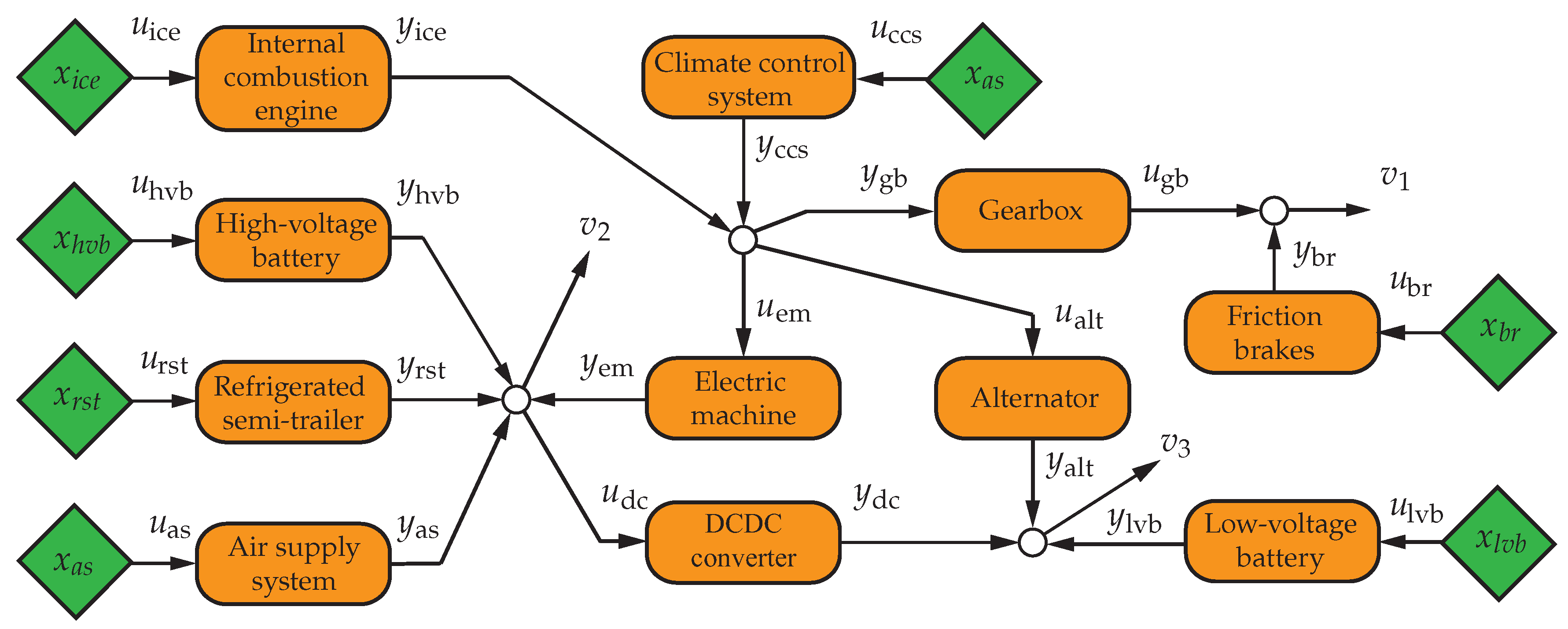
To demonstrate the flexibility of the power-based approach, we will consider a heavy-duty vehicle with several auxiliary systems, as schematically shown in Figure 1. The considered vehicle topology includes an internal combustion engine, an electric machine, an alternator, a high- and low-voltage battery, a refrigerated semi-trailer, an air supply system, a DC/DC converter, a climate control system, a gearbox and mechanical friction brakes. In this figure, is the (scalar) input power and is the (scalar) output power for . Furthermore, is the state for subsystem that represents the energy in the energy storage devices, which is only present for the dynamic subsystem , i.e., the high-voltage battery, the low-voltage battery, the refrigerated semi-trailer, the air supply system and the climate control system.
2.1. Objective and Topology
The objective in energy management is to minimize the cumulative fuel consumption, i.e.,
for , where is the fuel consumption rate that needs to be determined subject to all of the constraints acting on the vehicle and the subsystems in the vehicle. The constraints and subsystem models will be developed below. The fuel consumption of the engine typically depends on the engine output power and engine speed, i.e., , where the engine output (i.e., mechanical) power at time is defined as:
where is the engine torque at time t and is the engine speed at time . We can also define the engine input (i.e., fuel) power by:
where is the constant lower heating value of the fuel in . The definition of the engine input power allows (1) to be rewritten in a more general expression of minimizing the energy consumption, i.e.,
which has the same optimal solution as (1) because is a positive constant. In (3), the engine input power is a function of the engine output power and engine speed, i.e., for which an approximation is given in Section 2.2.1. Indeed, each of the subsystems in the heavy-duty vehicle can be expressed in terms of their input and output power as is shown in Figure 1. We will assume that the power losses in the gearbox are negligible, i.e., , so that the two nodes connected via the gearbox can be lumped together, and the remaining three nodes in the topology where power is aggregated can be described by:
where (4a) gives the aggregation of mechanical power at the mechanical side of the topology, (4b) gives the aggregation of high-voltage power at the high-voltage side of the topology and (4c) gives the aggregation of low-voltage power at the low-voltage side of the topology. In (4), , and are the disturbances acting on each node, which are the power required to follow a specified velocity profile, the power required for unmodeled high-voltage loads and the power for unmodeled low-voltage loads, respectively. These disturbance are predicted with the method presented in Section 4.
To complete the vehicle model for the topology given in Figure 1, a model is required for each of the subsystems that describes the input power , the output power for and the state for .
2.2. Subsystem Models
For each of the subsystems in the heavy-duty vehicle, the relation between the input and output power (,) is approximated with a quadratic equality constraint, i.e.,
with (time-dependent) efficiency coefficients , and . The input power is constrained to:
for , where is the set with the indices of the subsystems that can receive a continuous input power setpoint. The input power is constrained to:
for , where is the set with the indices of the subsystems that can only receive a discrete input power setpoint, e.g., the refrigerated semi-trailer can only be turned on or off. Furthermore, we model the energy in the subsystems with a linear differential equation of the form:
for all and with specific matrices , , and disturbance . The energy stored inside the subsystem is constrained to:
for . We will show below that each of the subsystems in the heavy-duty vehicle can be modeled in either of the forms (5).
2.2.1. Internal Combustion Engine, Electric Machine and Alternator
Similar to the definitions of input and output power of the internal combustion engine, given by (2), the input and output powers of the electric machine and alternator are defined as:
respectively. In these equations, is the electric machine torque, is the electric machine and alternator speed, which is proportional to the internal combustion engine speed, and are the voltages of the high- and low-voltage board net, respectively, and and are the current flowing through the electric machine and alternator, respectively.
With these definitions, the input-output power behavior of the internal combustion engine, the electric machine, and the alternator can be described by (5a), where the efficiency coefficients typically depend on the engine speed , i.e.,
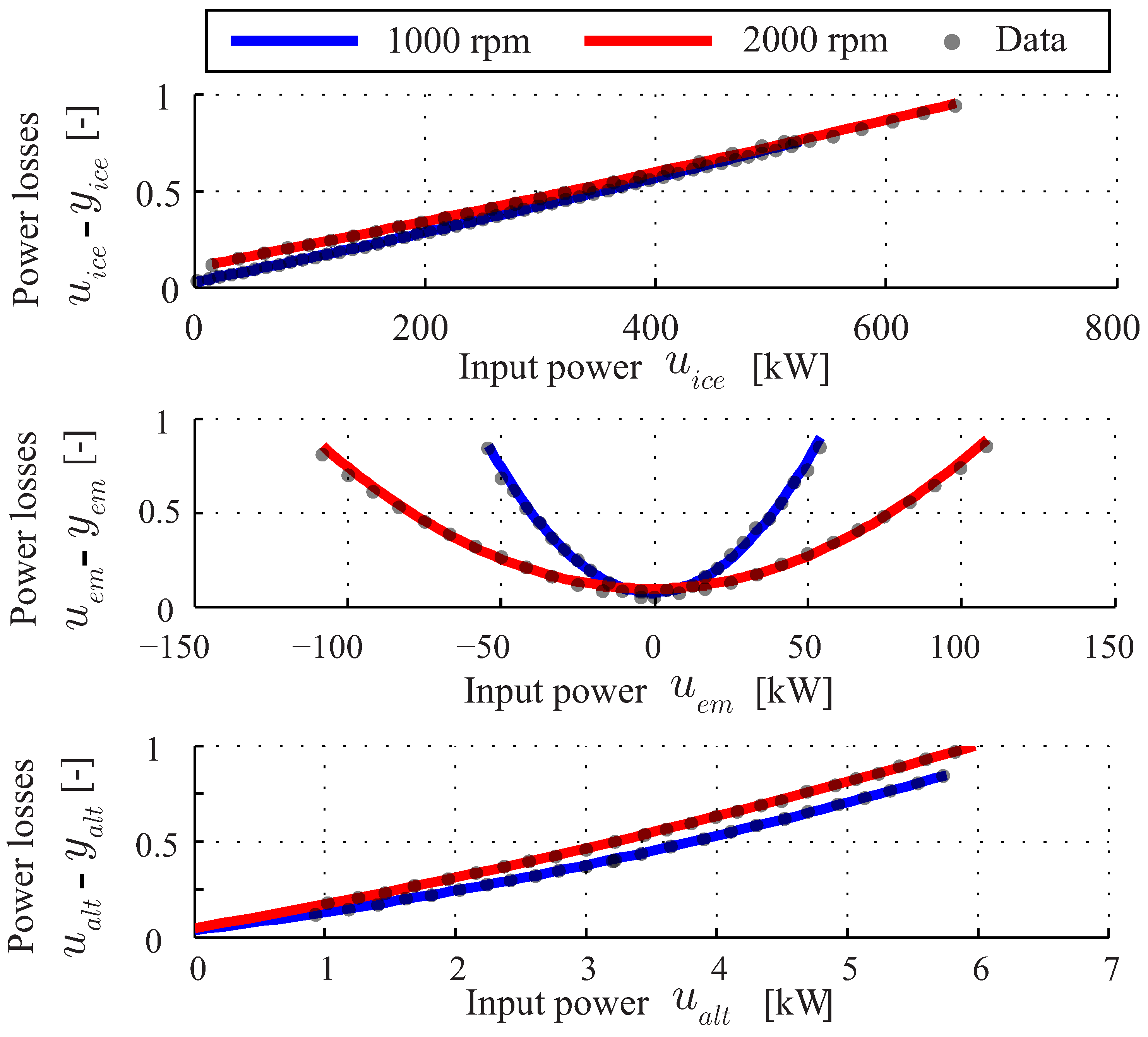
The accuracy of the quadratic approximation (5a) with (7) of these components is shown in Figure 2 for two engine speeds. The input power is constrained to (5b) for where the minimum and maximum input power also typically depend on speed .
2.2.2. DCDC Converter and Mechanical Brakes
The input and output power of the DCDC converter is defined by:
respectively, where is the DCDC current at the high-voltage side, is the DCDC current at the low-voltage side. The mechanical brakes are available for the case that not all energy can be recuperated by the other subsystems due to constraints. The output power is dissipated and a physical origin of the input and output power is therefore not necessary. Still, the input-output behavior for both, the DCDC converter and mechanical brakes, can be described by (5a) for with efficiency coefficients , and for that do not depend on speed. The input power is constrained to (5b) for where the minimum and maximum input power do not depend on speed.
2.2.3. High- and Low-Voltage Battery
The vehicle under consideration has a high-voltage battery connected to the high-voltage network and a low-voltage battery connected to the low- voltage network. The models of the high- and low-voltage battery are derived from a battery equivalent circuit model, i.e., an open circuit voltage for in series with a resistance for (see, e.g., [2]), which lead to an input-output behavior given by (5a) with , and for , which is bounded by (5b) for . The amount of energy in the high- and low-voltage battery, i.e., for satisfies (5d) for with , , and for and is constrained to (5e) for . It should be noted that the models used in this paper can be extended to have charge acceptance limitations. However, in [34], it has been shown that this does not lead to a significantly different energy management strategy.
2.2.4. Refrigerated Semi-Trailer
The thermal dynamics of the air inside the refrigerated semi-trailer is modeled using an energy balance given by:
where is the thermal capacity of the air in the refrigerated semi-trailer, is the air temperature, is the thermal power flowing into the refrigerated semi-trailer where negative powers indicate cooling, is a heat transfer coefficient between the ambient temperature and the air temperature and is an insulation coefficient. It is assumed that the temperature of the cargo remains within acceptable bounds as long as the air temperature remains within acceptable bounds. We can represent the refrigerated semi-trailer model in terms of stored energy by defining the thermal energy relative to the ambient temperature, i.e., so that the thermal energy satisfies (5d) for with , , and where the thermal energy is constrained by (5e) for .
The relation between the input and output power is approximated with (5a) for with suitable choices of , and and is constrained to (5c). The thermal power is not continuous with this constraint and this set is not a convex set, which is not attractive for optimal control. Therefore, a convex approximation is obtained by assuming (5c) holds instead of (5b) for and a solution for taking into account (5c) is proposed in Section 3.3.
2.2.5. Air Supply System
To limit the amount of states in the air supply system, the air vessels of the air supply system are lumped into one vessel with a lumped volume V and air pressure . The dynamics of the air pressure in the lumped system are assumed to satisfy a mass balance (see, e.g., [28]) given by:
where R is the specific gas constant for air, V is the lumped volume of the air tanks, is the mass flow into the air vessels with air temperature and is the mass flow out of the air vessels with air temperature . We can represent the air supply model in terms of stored energy by defining the pneumatic energy relative to the ambient pressure where is the ratio of specific heats (approximately 1.4 for air). Furthermore, we define the pneumatic input power by so that the pneumatic energy satisfies (5d) for with , , and and where the pneumatic energy is constrained to (5e) for .
2.2.6. Climate Control System
As in [35], only the evaporator in the climate control system is modeled, which is assumed to satisfy a set of coupled thermal energy balances given by:
where and are the heat capacities of the refrigerant and the walls of the evaporator, respectively, and are the temperatures of the refrigerant and walls of the evaporator, respectively, is the effective cooling power from the compressor, is the ambient temperature, and are the heat transfer coefficients between the inner and outer walls of the evaporator, respectively and is the heat generated when the inlet air is condensed (latent heat), which is assumed to only depend on the ambient air temperature and humidity . Similar to the battery, we can represent the climate control system model in terms of stored energy by defining the thermal energy in the wall and refrigerant relative to the ambient temperature, i.e,
which satisfies (5d) for with:
and . The energy in the climate control system is constrained to (5e) for . The relation between the input and output power is approximated by (5a) for with suitable choices of , that depend on the ambient temperature and internal combustion engine speed and and is constrained to (5c) for . Again, a convex approximation is obtained by assuming (5c) holds instead of (5b).
The convex approximation of the CVEM problem is now fully defined by the objective, the topology constraints, and the dynamics and constraints acting on each subsystem of the vehicle. In the next section, we propose to make a discrete time approximation of the CVEM problem with a prediction of the disturbances that is solved via a distributed model predictive control approach.
3. Distributed Economic Model Predictive Control
In this section, we propose to use a distributed economic model predictive control approach to efficiently solve the CVEM problem over a receding horizon. The solution is found by decomposing the optimal control problem with a dual decomposition, which results in multiple smaller optimization problems related to each component, which can be solved efficiently. This section first presents the receding horizon control problem, then the distributed solution approach followed by a method to handle on/off-controlled subsystems. Finally, we will discuss the stability and recursive feasibility properties.
3.1. Receding Horizon Optimal Control Problem
The objective for CVEM amounts to minimizing the cumulative fuel consumption, which is equivalent to minimizing the cumulative fuel energy given by (3). In this paper, the CVEM is solved in a receding horizon fashion, for which we approximate the objective function (3), at each given time instant by:
with prediction time instant where N is the prediction horizon and where the engine input power is assumed constant over the length of the sample interval . In model predictive control, (14) is solved over the horizon N at each fixed time instant . Only the first decision is implemented, i.e., is implemented at time . At the next time instant , this process is repeated and results in as the implemented control action at time . Note that the objective function (14) is only defined in variables related to the internal combustion engine. We therefore use the idea from [26] and define an equivalent objective function in variables related to every subsystem in the network, i.e., in the form of:
where and are the inputs and outputs of the converter in subsystem , which are constant over the length of the sample interval . In particular, the objective in (15a) is equivalent to (14) for for all , for and for as was shown in [26]. Therefore, by solving (15a), we solve the discrete-time approximation of (3). Note that, in (15a), we use the notation to indicate . This notation will be used throughout the paper for minimizing over a set.
The receding horizon optimal control problem aims at solving (15a) at each time instant subject to a quadratic equality constrained describing the input-output behavior of each converter, i.e.,
for and and subject to linear system dynamics of the energy in the storage device in subsystem m, i.e.,
for and and where is the measured current state of the storage device m, is a desired final state of the storage device m at the end of the prediction horizon, is a predicted disturbance at every prediction time instant at time for storage device m and subject to linear inequality constraints on the inputs of each converter, i.e.,
for all and and subject to linear inequality constraints on the states of each storage device, i.e.,
for all and . Finally, the optimization problem is solved subject to a linear equality constraint describing the interconnection of the subsystems, i.e.,
for all , where and and are vectors with the ℓ-th element being if the power flow to the node ℓ is positive, 0 if there is no power flow to the node ℓ, 1 if the power flow to the node is negative. Here, L is the number of nodes in the topology where power is aggregated. Indeed, the power balance constraints in (4) are given by (15f) for well chosen matrices and . Furthermore, it is assumed that the disturbance can be measured at each time instant , while for has to be predicted at each time instant with the prediction algorithm presented in Section 4.
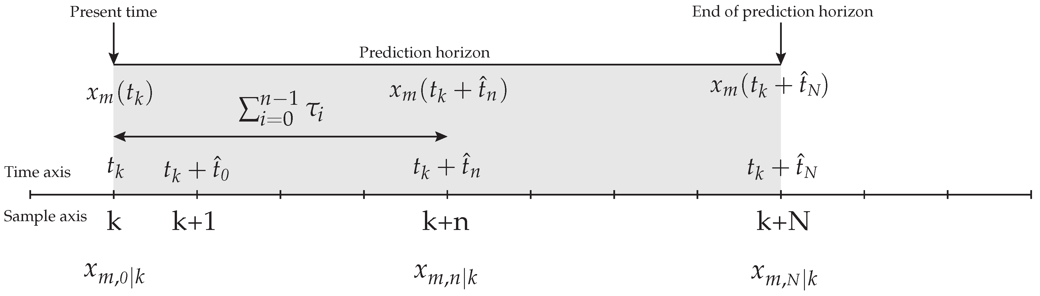
It should be noted that the efficiency coefficients , and and the upper and lower bounds and , respectively, that depend on speed, as is the case for the internal combustion engine, the electric machine and alternator, are obtained by evaluating these coefficients and bounds at the predicted speed for at each time instant . Moreover, the dynamics of the high- and low-voltage battery, the refrigerated semi-trailer, the air supply system and the climate control system can all be formulated as a linear differential equation, i.e., (5d) for . This differential equation allows us to make a prediction of at some future time (see Figure 3), where , given a measurement of the state at present time and a piecewise constant , i.e., for and . This prediction is made by making a discrete approximation of (5d), leading to (15c) with:
in which and is the sample time used in (5d).
In [33], we proposed to take variable prediction time intervals to allow for a long prediction horizon using only a limited number of prediction instants N. This is necessary to keep the optimal control problem small in the number of decision variables and real-time solvable. This method is similar to move blocking strategies [36] except that it does not only assume that the control inputs over the prediction time intervals are constant, it also assumes that it is sufficient to only constrain the dynamics at the beginning and end of each interval through (15c).
3.2. Distributed Solution Using a Dual Decomposition
The optimal control problem (15a) subject to (15b)–(15f) is a quadratically constrained linear program, which cannot be easily solved using embedded solvers, e.g., CVXgen [37] or QPoases [38]. We therefore apply ideas from distributed optimization and will show that this leads to several linearly constrained quadratic programs (LCQPs). It should be noted that the subsystems in (15) are only connected by (15f).
To decompose the problem, we will employ the dual decomposition approach, as was done in [26]. Using the notation of this paper, we augment the objective function (15a) with the complicating constraints (i.e., the constraints that act on more than one subsystem), which is (15f) in this case. This leads to the following so-called partial Lagrangian:
where is a Lagrange multiplier, which is to be solved subject to (15b)–(15e). The partial Lagrange dual function is given by:
with:
subject to (15b)–(15e). Note that each of the Lagrange dual functions (18b) subject to (15b)–(15e) is related to one of the subsystems and can be solved independently. To solve the dual optimization problem, the dual function (18) has to be maximized over . This can be done using a ‘steepest ascent’ method by iteratively solving:
where is a suitably chosen matrix. It has been shown in [26], that under very mild and verifiable conditions, the optimal values of the dual optimization problem (18) and (19) and the primal optimization problem (15) are the same.
Each of the Lagrange dual functions (18b) related to one of the subsystems can be solved separately and can be written as an LCQP by substituting (15b) into (18b), which gives:
with:
and subject to (15c)–(15e). Note that for convexity of (20a), it is required that for all , . Under this condition, the dual decomposition allows solving the quadratically constrained linear program by solving multiple LCQPs iteratively. These LCQPs can be solved efficiently in real-time using, e.g., CVXgen [37] or QPoases [38].
The dual decomposition leads to a distributed economic model predictive control approach for CVEM that can be summarized in the following algorithm where is a well chosen convergence criteria, is the iteration counter and is the maximum number of iterations.
| Algorithm 1: Distributed economic model predictive control approach for CVEM. |
Take and initialize . Set , .
|
3.3. Modified Lagrange Dual Function for On/Off Control
For the optimal control problem presented so far, it has been assumed that the decision variables for all and all are constrained to an interval given by (15d). However, for some subsystems introduced in Section 2, the power can only be turned on or off, i.e.,
for all and where and correspond to the power consumption when the auxiliary is off and on, respectively. The optimal control problem (15) subject to (21) instead of (15d) for is hard to solve due to the binary decision variables. To still allow on/off control for some of the subsystems, we approximate the solution of (15) subject to (21) instead of (15d) for by a solution for which we only take (21) for and take (15d) for , i.e., (21) is relaxed to being an element of a continuous interval for the tail of the horizon. This approximation is justified as only the first element of the decision variables is actually used as a setpoint for the power to a subsystem. To do so, we augment (20) with a penalty for switching from on to off and vice versa, i.e.,
where the Lagrange dual function for which is given by:
and where the Lagrange dual function for which is given by:
with , and as defined in (20b)–(20d), subject to (15c)–(15e) and subject to (21) instead of (15d) for . In (22), indicates whether the subsystem is currently on or off and is a (state-dependent) penalty parameter. This penalty parameter is used to achieve a desired switching frequency.
The optimization problem (22) can now be solved by solving the two LCQPs (22b) and (22c) and the optimal decision at the first time instant () is given by:
It is this control action that is implemented at time instant for this subsystem . It has to be noted that the optimal control problem (15) subject to (21) for and (15d) for is not convex and consequently it is not guaranteed that the dual solution will converge to the primal solution . However, in case that the power of the on/off (non-convex) subsystems is small compared to the continuous (convex) subsystems, the dual solution will still converge for most time instances and a close to optimal performance can be achieved. This will be demonstrated in Section 5.
3.4. Stability and Feasibility
Stability and feasibility are generally important properties that need to be addressed for MPC. Stability, however, is not a concern for the economic MPC approach presented in this paper. Namely, the objective is not to control the states to a steady-state value, but to find a solution that minimizes the energy losses in the vehicle while satisfying the upper and lower state constraints over a finite horizon.
Still, feasibility does need to be addressed. The following three causes can lead to an infeasible solution:
- The CVEM problem becomes infeasible if the power of the internal combustion engine is not sufficient to provide power to all subsystems and disturbances in the vehicle.
- The optimal control problem related to one of the subsystems becomes infeasible if the final state cannot be reached due to limitations on the control inputs and a horizon that is not sufficiently long.
- The optimal control problem related to one of the subsystems becomes infeasible if the initial state at time instant violates the state constraints as a result of unpredicted disturbances and modeling errors.
The first cause for infeasibility can be avoided by having a sufficiently powerful internal combustion engine that can always provide enough power to all subsystems and disturbances in the vehicle. In practice, it can occur that the engine power is limited, which eventually would lead to a degradation of driveability.
The second cause for infeasibility can be avoided by taking a sufficiently long horizon. An indicative measure for the minimal length of the horizon for each of the dynamic subsystems can be obtained by maximizing the lower bound on the required control horizon . This lower bound should be such that there exists an input for such that:
for both and (an estimate of) the worst-case disturbance and the given final state . With the variable prediction time intervals proposed in this paper, the horizon can be taken sufficiently long, so as to satisfy (24), without the need for many decision variables.
The third and final cause for infeasibility can be solved by projecting the initial state into the feasible set and contracting the input constraint (15d) for to ensure feasibility for the next time instant. Note that, as a result, it is not guaranteed that the state constraints will not be violated. For CVEM, this is not a concern as the state constraint are already chosen conservatively from practical considerations and small violations of the state constraints is allowed.
4. Prediction of Disturbance Signals with ADASIS
In order to solve the CVEM problem with the DEMPC approach, accurate predictions of the disturbances , , and , as in (15c) and (15f), are needed, as well as time varying efficiency constants in (15b), which requires an accurate prediction of the engine speed . In this paper, we assume that all disturbances at the energy storage buffers are constant (i.e. for all and ) and measurable, e.g., the ambient temperature of the refrigerated semitrailer, see Section 2. Furthermore, we assume that the high-voltage network has no disturbances, i.e., for all and and the disturbance power on the low-voltage network (consisting of e.g., the power needed for the head lights) is identified online. The latter is done by considering the optimal solution at time instant and finding the value , for that satisfies (4). As a result, we only need a method to obtain an accurate prediction of the propulsion power , i.e., the power needed at the wheels for tracking a reference velocity and the engine speed .
4.1. Power Required at the Wheels
The propulsion power and the engine speed at prediction step at time are obtained by averaging the prediction of the propulsion power and engine speed, i.e.,
for with , , and . The propulsion power and engine speed depend on the road slope , the vehicle speed and the selected gear and can be predicted using a simple longitudinal vehicle model (see, e.g., [3]). In particular, we predict these quantities using:
where is the combined gearbox and differential ratio that depends on the selected gear , is the dynamic wheel radius, is the (predicted) vehicle speed, m is the vehicle mass, is the equivalent inertia of the drive line at the wheels as function of the selected gear, g is the gravitational constant, rolling resistance coefficient of the tires, A is the frontal area, is the air drag coefficient and is the air density. It is assumed that all constants are known, or can be estimated online using techniques presented in [39,40,41,42]. The time dependent road slope , vehicle speed and gear selection , however, need to be predicted for .
4.2. Prediction Algorithm
The road slope can be predicted with an e-horizon system, such as the advanced driver assistance system ADASIS, see [43], which gives a vector of road slopes over the relative distance to the current position of the vehicle, i.e., . Prediction of the velocity is more difficult. Nevertheless, since we consider long-haul heavy-duty vehicles, which spend most of their time on the highway, we can assume that the cruise control (CC) or the downhill speed control (DSC) is active during most of the driving. In this case, the desired velocity of the vehicle is regulated towards for cruise control and towards for downhill speed control. Typically, it holds that , i.e., the DSC speed is higher than the CC speed, which allows some of the potential energy to be stored as kinetic energy. Finally, a rule-based gear shift strategy is assumed that satisfies:
were is the constant lower threshold for gear shifting, respectively. This strategy seeks always the highest gear for which the minimum engine speed is satisfied, which corresponds generally with the most efficient gear shift strategy. The propulsion power is constrained as well:
where and are the lower and upper bound that depend on the vehicle speed, the selected gear and whether CC or DSC is active. In particular, the maximum power is always constrained to the maximum engine power, i.e.,
where is the efficiency of the gearbox and differential as function of the selected gear. The minimum power is constrained to:
This constraint means that braking with the electric motor and friction brakes is only allowed when the vehicle speed exceeds the desired downhill speed.
Solving (26) subject to (27) and (28a) is hard due to the nonlinear vehicle dynamics, the appearance of the derivative and the constraints (28) and because the road slope is given as function of distance and not as function of time. Therefore, we propose to make a forward Euler approximation of (26) over the time horizon at time instants , . This includes approximating:
We then find a solution for (26) subject to (27) and (28a) sequentially over the interval and at each time instant we switch, if necessary, between CC and DSC and select a different gear. The algorithm to predict the power request at the wheels is then given by:
| Algorithm 2: Prediction of the power request and engine speed. |
Initialize and measure , . For ,
|
This algorithm predicts the power request and engine speed over the prediction horizon , which is used in (25) to obtain the average propulsion power and the average engine speed over the variable prediction time intervals for . This allows the optimal control problem (15) to be solved with the distributed model predictive control approach, as will be demonstrated in the next section.
5. Simulation Results
In this section, the results of the DEMPC approach to CVEM will be presented. We will focus on three aspects. The first aspect is the fuel saving potential of the distributed control approach, which is demonstrated by using the algorithm in a simple and predictable simulation environment. As prediction information is a key element in the proposed approach, the second step demonstrates the approach by using a high-fidelity vehicle model, where the power request and engine speed are predicted as in Algorithm 1. Finally, to demonstrate the real-time aspects of the algorithm, we will show the computational performance of the algorithm for a dSpace Autobox (dSPACE GmbH, Paderborn, Germany).
5.1. Fuel Saving Potential on a Low-Fidelity Vehicle Model
The energy management problem is solved in a receding horizon fashion as in Section 3, where at each time instant k the first input is implemented on the simplified power-based vehicle model introduced in Section 2. The vehicle model runs at a frequency of 1 Hz where the exogenous disturbances, e.g., the drive cycle are piecewise constant at each time step. In particular, the drive cycle is obtained by simulating the high-fidelity vehicle model over two parts of a PAN European driving cycle to obtain the power required at the wheels, i.e., and the engine speed which are shown in Figure 4. The second part has more braking moments than the first part, which has an influence on the fuel reduction. Furthermore, the uncontrolled high-voltage auxiliaries are assumed to be absent so that kW and the power required from uncontrolled low-voltage auxiliaries is assumed to be constant, i.e., kW.
We will first analyze the influence of the prediction horizon. Subsequently, we will give the results on the control of auxiliaries that can only be turned on or off and, finally, the influence of the number of iterations on the fuel reduction potential. The simulations done in this section will be benchmarked with the fuel consumption results of [26] and will be performed under the same conditions. The state trajectories of the simulations presented below do not deviate noticeably from the state trajectories presented in [26] and will therefore be omitted.
5.1.1. Influence of Prediction horizon
A key element in the proposed algorithm is the variable prediction time intervals that allow for a large control horizon with a few decision variables. Choosing the length of these variable prediction time intervals is not straightforward, but we will demonstrate that choices can be made based on practical limitations and intuition, while close to optimal performance can be achieved. To do so, we first consider the case of a hybrid electric truck without auxiliaries and predict the power at the wheels, i.e., for all at time instant k and the engine speed for all at time instant k with (25), where and are given as in Figure 4. We will consider three different cases with decreasing level of prediction information, i.e.,
- Case 1: In this case, we do not take variable prediction time intervals, but take intervals of 1 s, i.e., . Because the simulation model has a sample time of 1 s, we have that the prediction is exact over the length of the interval . This also means that N is large to obtain a large control horizon. Real-time implementation is therefore not feasible and this case can only be solved for a hybrid truck without taking the auxiliaries into account in the energy management strategy.
- Case 2: In this case, we do take variable sample intervals with and predict the propulsion power and engine speed with (25). We choose from a practical point of view as 80 s corresponds to about 2 km of prediction information at cruise control speed (84 km/h). This is the maximum distance over which prediction information is currently available with ADASIS in the prototype heavy-duty vehicle. To still allow for a larger control horizon, we can choose for which in this case the power at the wheels and the engine speed is calculated with (25) as well.
- Case 3: This case is a small adaptation to Case 2. Namely, as prediction information is not available after 80 s (in practice), the propulsion power and the engine speed for , i.e., and , [-10]cannot be predicted and is therefore assumed to be fixed to a pre-specified value after 80 s.
The choice for the sampling time intervals for Case 2 and Case 3 is based on three considerations, i.e., (i) s, (ii) The first interval is 1 s as this decision is implemented, (iii) The intervals should increase in size as , as nearby prediction information is likely to be more accurate. These considerations do not lead to too many significantly different choices for the sequence , and the results in Figure 5 show that good performance can be achieved with the one proposed. In this figure, the fuel reduction is shown as function of the horizon length for each of the three cases and for the two parts of the drive cycle. The horizon length for Case 1 is changed by changing N while for Case 2 and Case 3, the horizon length is changed by changing . Moreover, the global optimal solution is calculated with the approach presented in [26] and shown as a constraint. Note that for Case 3, the power request after 80 s is fixed to a pre-specified value. Therefore, it is not useful to choose the horizon very long for Case 3 as this results in a lower fuel reduction. Figure 6 shows the simulation results for Case 3 for three different horizon lengths and where the power request after 80 s, i.e., , is varied from 10 kW to 90 kW and rpm. The main conclusion drawn from these two figures is that Case 3, which is closest to practice, can achieve good fuel reduction performance and sensitivity to the length of the control horizon and the choice for is not significant. For the remaining simulations, we choose , kW and rpm.
These settings also fully define the smart control of the continuous controlled alternator. Smart control of the alternator (without a DCDC converter) leads to a fuel reduction of and fuel reduction for Part 1 and Part 2, respectively. By adding smart control of the DCDC converter, the fuel reduction is increased to and for Part 1 and Part 2, respectively. Smart control of the auxiliaries with on/off control will be discussed in the next section.
5.1.2. Auxiliaries with On/Off Control
Next, we consider the analysis of the on/off controlled auxiliaries. The simulation results are obtained by taking only the hybrid vehicle with one additional switching subsystem, e.g., the refrigerated semi-trailer. Note that this requires solving two QPs for every switched system at each time instant k. We have defined three different switching strategies, i.e.,
- Strategy 1: For this strategy, the penalty parameter for switching is a constant value.
- Strategy 2: Inspired by [44], the penalty parameter for switching is defined by where is a target state and is a positive weight. The target state is the lower energy bound if the subsystem is off and the target state is the upper energy bound if the subsystem is on.
- Strategy 3: This strategy is a small adaptation of Strategy 2 and only used for the refrigerated semi-trailer and air supply system. Here, the desired final state in the energy storage device is adapted as a linear function of the average value of the dual variables, i.e., for some a and b and where the average value of the dual variables over the prediction horizon is given by . This can improve the performance of subsystems with a default switching time much larger than the prediction horizon, such as the refrigerated semi-trailer and air supply system.
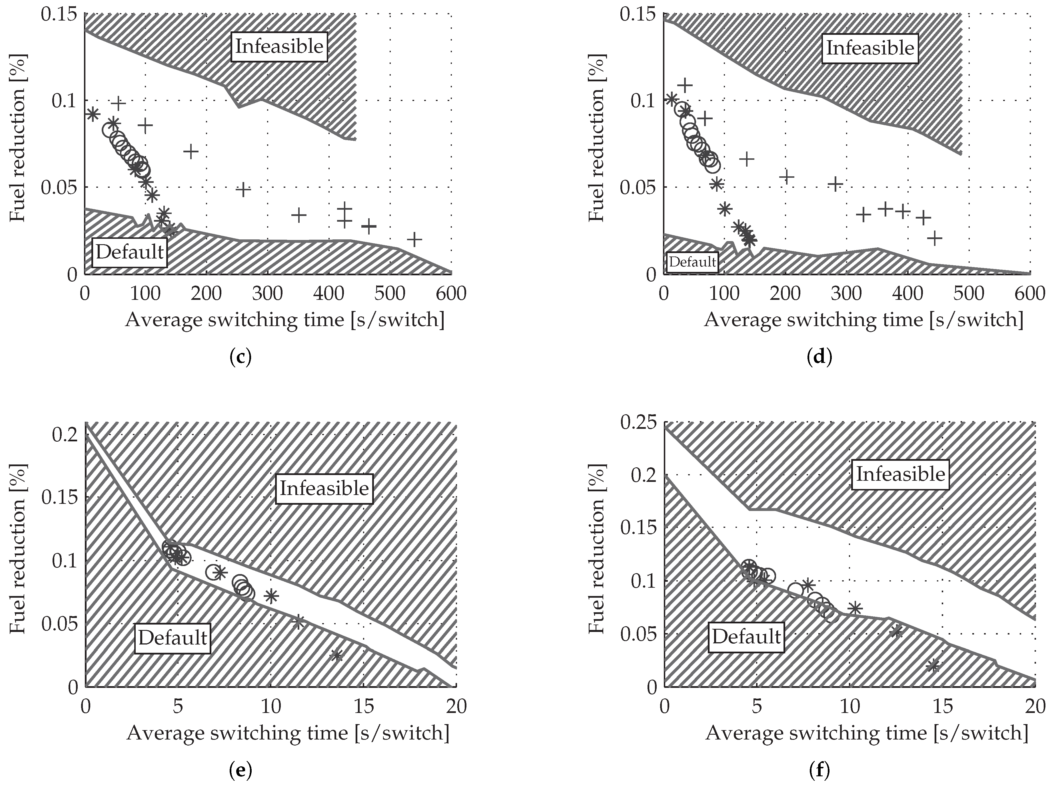
The fuel consumption with each of these strategies is compared to the fuel consumption with a default controller, which switches between a fixed upper and lower bound. For the refrigerated semi-trailer, the temperature cycles between 4.5 °C and 5.5 °C. For the air supply system, the air pressure cycles between 9.6 bar and 13.1 bar and for the climate control system, the wall temperature of the evaporator cycles between 9 °C and 13.5°C. The results for each of these strategies and each of the subsystems are shown in Figure 7 for Part 1 (a,c,e) and Part 2 (b,d,f) of the drive cycle. Different penalty parameter settings are used, which result in a different average switching time. Figure 7 shows a feasible region for real-time control in between the two hatched regions, i.e., the infeasible region and the default controller region. The upper boundary of the feasible region is given by the optimal trade-off between the number of switches and the fuel reduction and obtained with dynamic programming [45]. The default controller turns on the auxiliary when the lower energy limit is violated and turns the auxiliary off when the upper energy limit is violated. For these auxiliaries, it holds that the more energy is stored, the higher is the rate of energy dissipation to the environment. To show this, let us consider the example of a refrigerated semi-trailer, where a larger difference between the air temperature inside and the ambient temperature outside leads to a larger energy dissipation. By decreasing the upper energy limit, the number of switches with default control will increase, but also the energy dissipation reduces leading to a fuel reduction. This trade-off defines the lower boundary of the feasible region, which lowers the potential fuel reduction by smart on/off control for these auxiliaries. Still, a significant amount of fuel can be saved with the refrigerated semi-trailer, the air supply system and the climate control system, but the average switching time is also significantly lower.
For the refrigerated semi-trailer and the air supply system, it is very difficult to obtain a large average switching time as the switching time intervals easily exceed the maximum length of accurate prediction information. The climate control system is difficult to optimize as the fuel reduction for the default control strategy with a lower switching time is already quite high compared to the maximum obtainable fuel reduction.
5.1.3. Number of Iterations
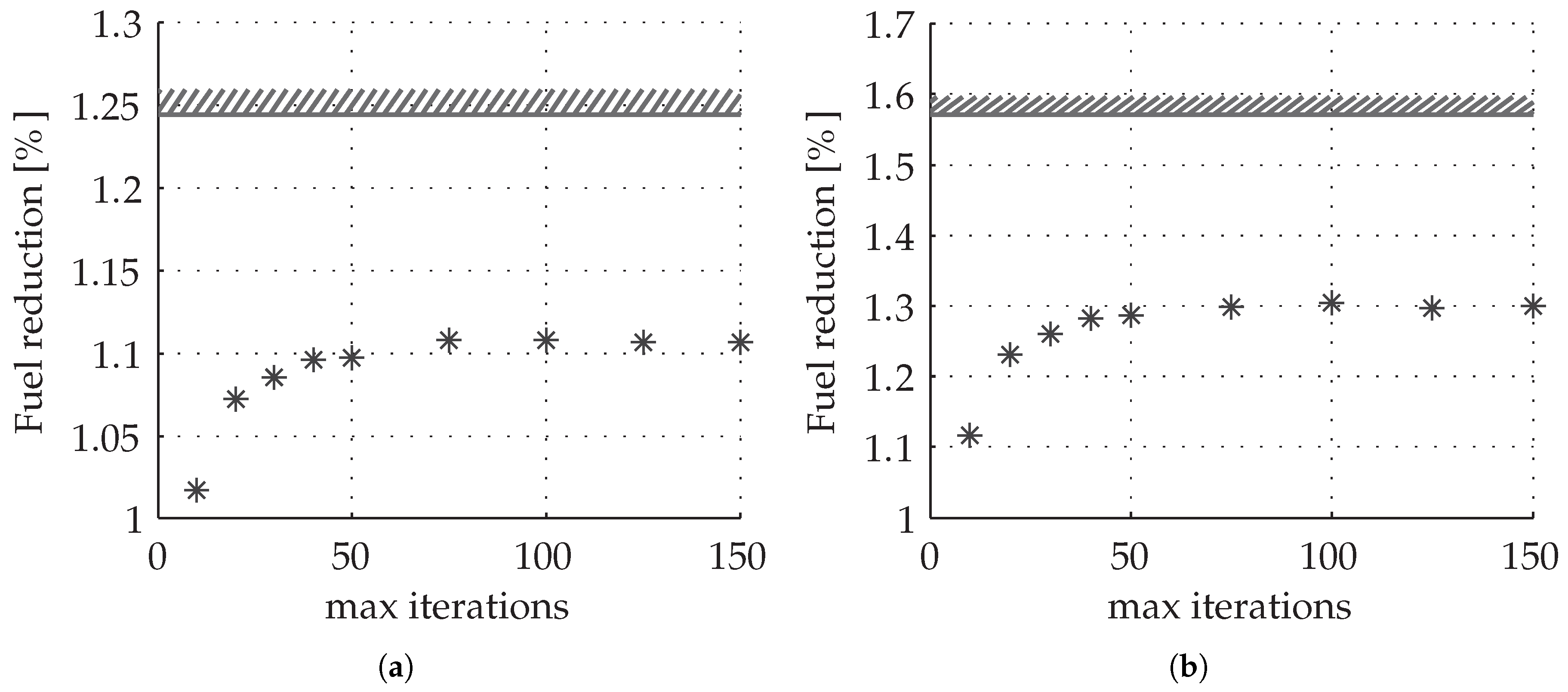
So far, the number of iterations in (19) for all the simulations do not have an upper bound. However, at each iteration, eight LCQPs need to be solved so that limiting the amount of iterations reduces the computation time and thereby improves the real-time properties. Therefore, smart control of the hybrid vehicle with all auxiliaries is simulated subject to a maximum on the number of iterations. The fuel reduction results by smart control of the auxiliaries are shown in Figure 8 for Part 1 and Part 2 of the drive cycle. Only the fuel reduction of the smart auxiliaries are shown to demonstrate the potential of CVEM. The average switching time for the refrigerated semi-trailer is 35 and 22 s for Part 1 and Part 2, respectively, for the air supply system 52 and 31 s, for Part 1 and Part 2, respectively, and for the climate control system 7 s for both parts of the drive cycle. With a very low number of iterations, fuel reduction performance is indeed sacrificed, but the maximum fuel reduction performance is already achieved with an upper limit of 75 iterations, around 99% of the maximum fuel reduction is obtained with 50 iterations and around 97% of the maximum fuel reduction is obtained with only 25 iterations.
5.2. Validation on a High-Fidelity Vehicle Model with ADASIS Preview Information
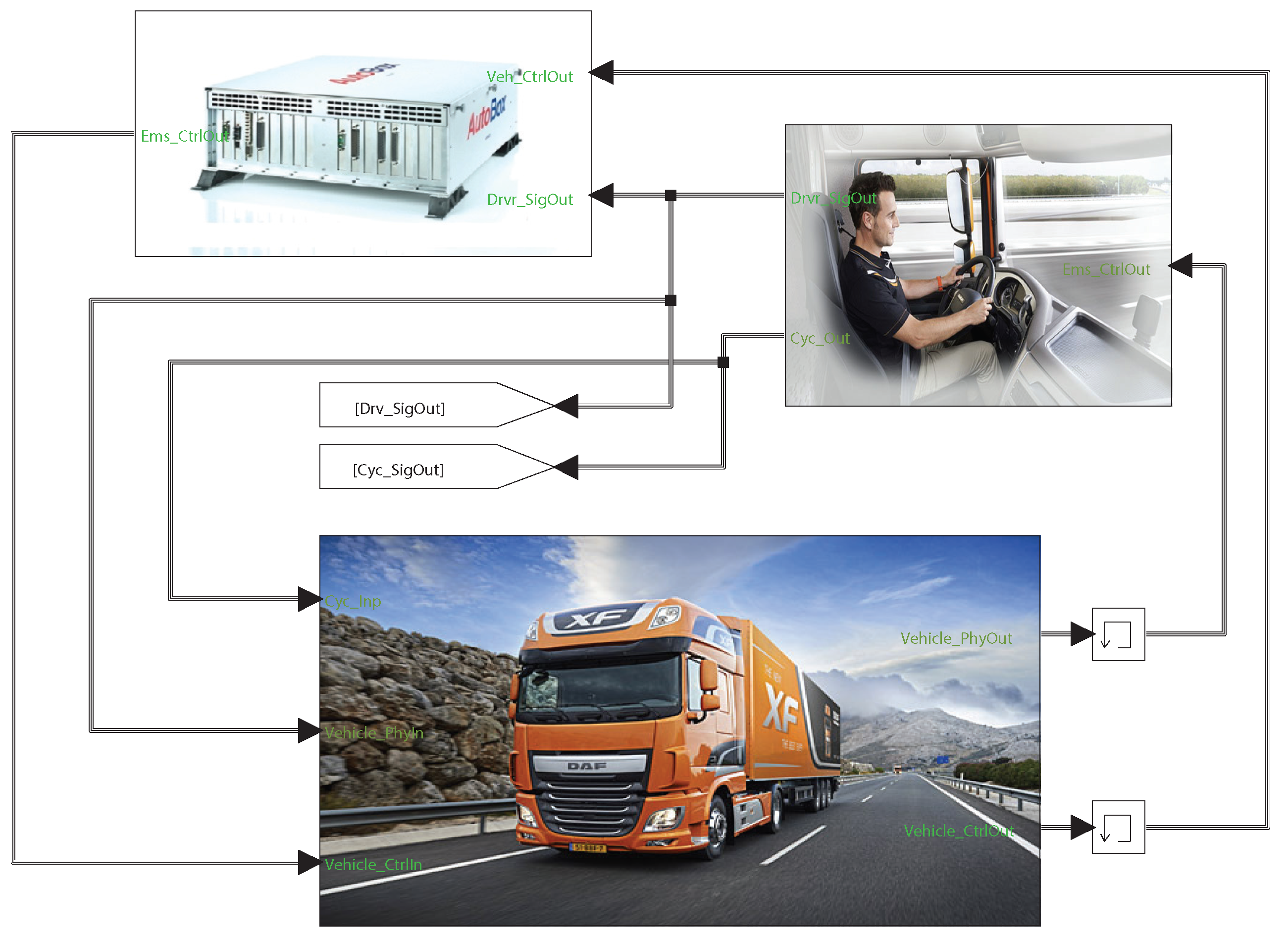
A prototype vehicle has been built, which has a hybrid drive train with an internal combustion engine and an electric machine attached to a high-voltage battery system and all auxiliaries are electrified. At the moment of writing this paper, the prototype vehicle is not approved to be tested on the public road, but only on designated test tracks. This constrains the validation of the online solution strategy as prediction information is not available for driving on the test track. Namely, prediction information is essential to demonstrate the fuel reduction potential of the DEPMC strategy. Therefore, the DEMPC strategy is validated on a high-fidelity vehicle model (see Figure 9) of the heavy-duty vehicle. The vehicle model is developed by the Institute für Kraftfahrzeugen Aachen (IKA, Aachen, Germany) [46,47]. It consists of a detailed vehicle model describing the longitudinal dynamics of the vehicle and the more-detailed (nonlinear) dynamics of all components in the vehicle.
The DEMPC strategy provides a setpoint to all subsystems in the vehicle, including the electric machine and internal combustion engine. However, control of the electric motor and internal combustion engine is difficult as safety is critical for a vehicle that weighs up to kg. Control of the hybrid system with DEMPC is therefore not feasible in the prototype vehicle. Therefore, it is decided to validate the strategy without control of the hybrid power split in the high-fidelity vehicle model as well. Still, the power required at the wheels can become negative, meaning that braking energy will be regenerated by the hybrid power split and stored in the high-voltage battery. This power can be used by the other subsystems, i.e., the refrigerated semi-trailer, the air supply system, the climate control system, the DCDC converter and the alternator, which receive setpoints from the DEMPC strategy. This still allows validation of the fuel reduction potential for most of the subsystems in the heavy-duty vehicle. The hybrid system is still an essential part of the DEMPC strategy, as the auxiliaries need the decisions from the hybrid system to optimize their own decisions. By doing so, the algorithm predicts the behavior of the hybrid system by assuming that the hybrid system will make the optimal decisions along the objective function in the optimal control problem.
5.2.1. Prediction of the Power Request and Engine Speed
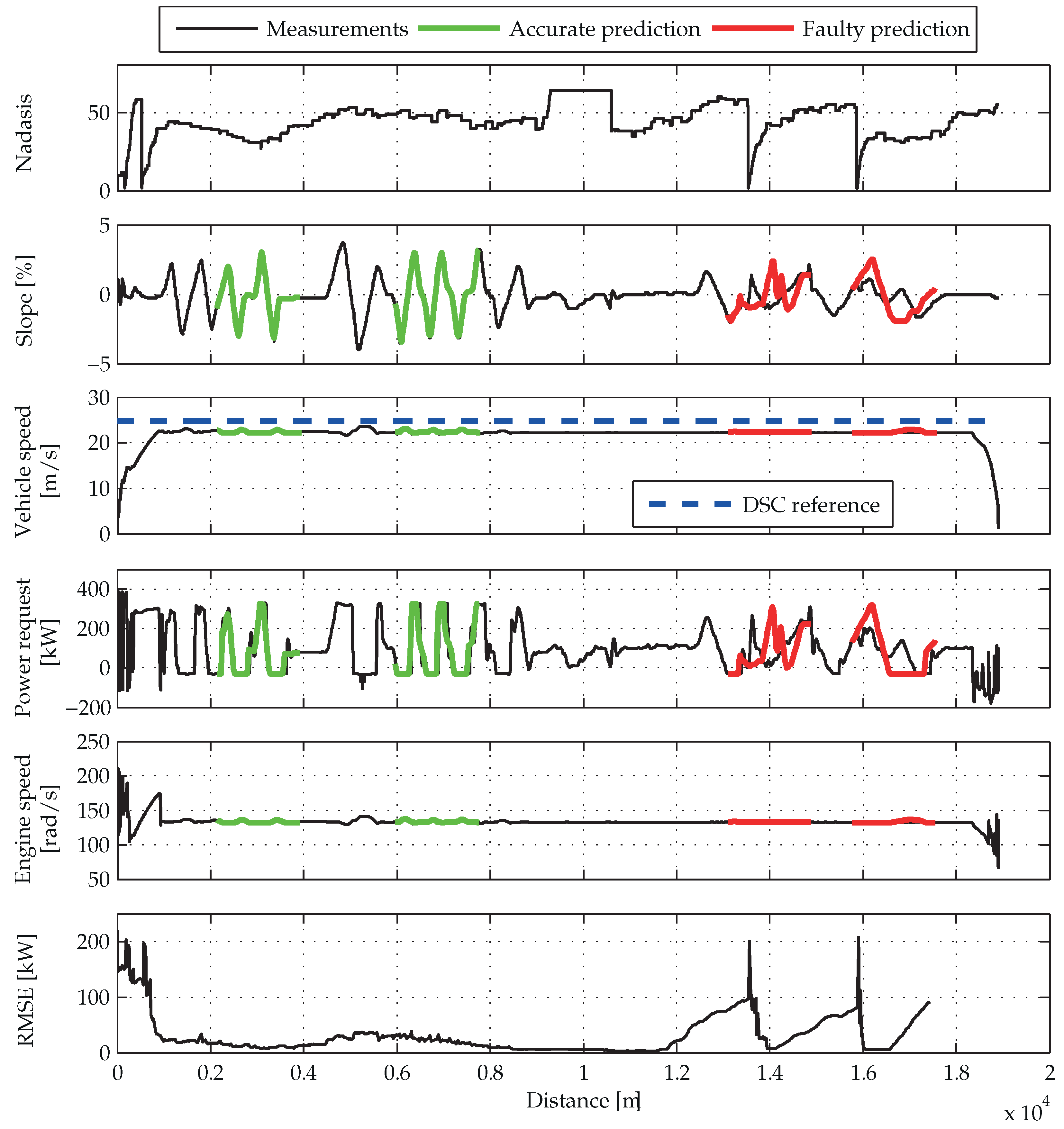
In the prototype vehicle, the road slope is predicted by the ADASIS protocol, which gives the road slope as function of the relative distance from the current position of the vehicle. ADASIS measurements are gathered for a highway cycle of 19 km driven in the region of Eindhoven (Netherlands). ADASIS provides the road slope at non-uniform distances from the current position. Moreover, the future road slopes are not instantly available but come available as a receding horizon based on the most probable path predicted by ADASIS.
The amount of predicted road slopes, indicated with therefore changes all the time as shown in Figure 10. The upper plot in this figure shows the number of predictions as function of the distance driven by the vehicle in the high-fidelity simulation environment. It can be seen in this figure that the power request is predicted in a consistent way, e.g., when the road slope becomes negative, the vehicle speed increases and the power request becomes negative. Occasionally, the number of predictions goes to zero, which happens when the vehicle takes an unexpected exit, i.e., the vehicle deviates from the most probable path predicted by ADASIS. After the exit, the ADASIS protocol notices that a different path is taken and all erroneous predictions are discarded. This happens three times on the drive cycle under consideration. The measured road slope and four examples of a road slope prediction by ADASIS are shown in the second plot. For the green labeled examples, plenty of predictions are available and no unpredicted exit is taken, which lead to very accurate prediction of the road slope. For the red labeled examples however, unpredicted exits are taken in the future, which result in a faulty prediction of the road slope. As a consequence, the velocity, the power request and the engine speed predicted with Algorithm 2, is quite accurate for the green labeled examples but faulty for the red labeled examples. This is also shown by the plot with the average root mean square error (RMSE) of the difference between the predicted power request and the measured power request over the entire prediction horizon. This plot clearly shows that if the vehicle follows the most probable path, an accurate prediction of the future power request can be made with Algorithm 2 in combination with the ADASIS protocol. As heavy-duty vehicles often tend to drive the same route, the protocol can and will be improved in coming years by taking this information into account for predicting the most probable path.
The drive cycle for which ADASIS information is available is very short and the area around Eindhoven is very flat so that differences in road slope are mainly caused by driving up and down flyovers. The differences in road slope are not even significant to reach the downhill speed control (DSC) reference speed after which the vehicle starts to actively recover brake energy with the hybrid system. This cycle will therefore not show the true potential of the DEMPC approach to CVEM. Instead the fuel reduction is analyzed with the high-fidelity vehicle model by driving the same drive cycle as used for the low-fidelity vehicle model. We will assume that the vehicle always follows the most probable path, i.e, the road slope prediction is exact. This leads to an average RMSE of 29 kW for the power prediction, which is similar to the RMSE made with the ADASIS protocol and Algorithm 2.
5.2.2. Fuel Reduction Results
The fuel reduction results with DEMPC approach are given in Table 1. To analyze the fuel reduction contribution of each of the subsystems, the results of various simulations are shown for which only one subsystem is being controlled with the DEMPC approach. The fuel reductions are given for Part 1, i.e., for and for Part 2, i.e., for . These are the same parts used to evaluate the control strategy on the low-fidelity vehicle model. For a complete analysis, the difference in stored energy inside the energy storage systems at the start and end of the cycle must be taken into account. However, as each of these drive cycles is very long, the effect on the overall fuel consumption is small and neglected in this table.
The fuel reduction is strongly related to the average switching time for the refrigerated semi-trailer, the air supply system and the climate control system. Compared with the default control strategy, the average switching time is decreased with a factor 8.5, 82 and 1.5 for the refrigerated semi-trailer, the air supply system and the climate control system, respectively.
For these average switching times the fuel reduction obtained with CVEM in the high-fidelity vehicle model is around half the fuel reduction obtained with the low-fidelity vehicle model. The amount of regenerative energy harvested on the low-fidelity vehicle model is, for all subsystems, larger than for the high-fidelity vehicle model, which can explain some of the differences in the fuel reduction. In particular, the energy harvested by the electric machine in the high-fidelity vehicle model is 25.8% lower than in the low-fidelity vehicle model due to, e.g., power restrictions caused by the time needed for gear shifting in the high-fidelity vehicle model. This has a significant impact on the fuel reduction potential of CVEM. Furthermore, comparing percentages is difficult as the fuel consumption for the default control strategy is 10.7% higher in the high-fidelity vehicle model than in the low fidelity vehicle model.
5.3. Implementation on the dSpace Autobox
As a final step to prove feasibility of the DEMPC approach to CVEM, the algorithm is implemented on a dSpace Autobox. The prototype vehicle is equipped with a dSpace Autobox with a DS1005 PPC Board (dSPACE GmbH, Paderborn, Germany) that features a PowerPC 750GX processor (dSPACE GmbH, Paderborn, Germany) running at 1 GHz. To test the real-time aspects of the control algorithm proposed in this paper, the algorithm is implemented onto the DS1005. The algorithm is running in open loop, i.e., the inputs for the control algorithm, e.g., the vehicle velocity, distance are not following from the vehicle model, which is too large to run in real-time, but follow from lookup tables. Similarly, the setpoints generated by the control algorithm are not implemented on the vehicle model but are discarded. Still, the ADASIS information is processed in real-time as function of the distance driven by the heavy-duty vehicle. This approach allows us to isolate the computational performance of the previewer and the control algorithm only.
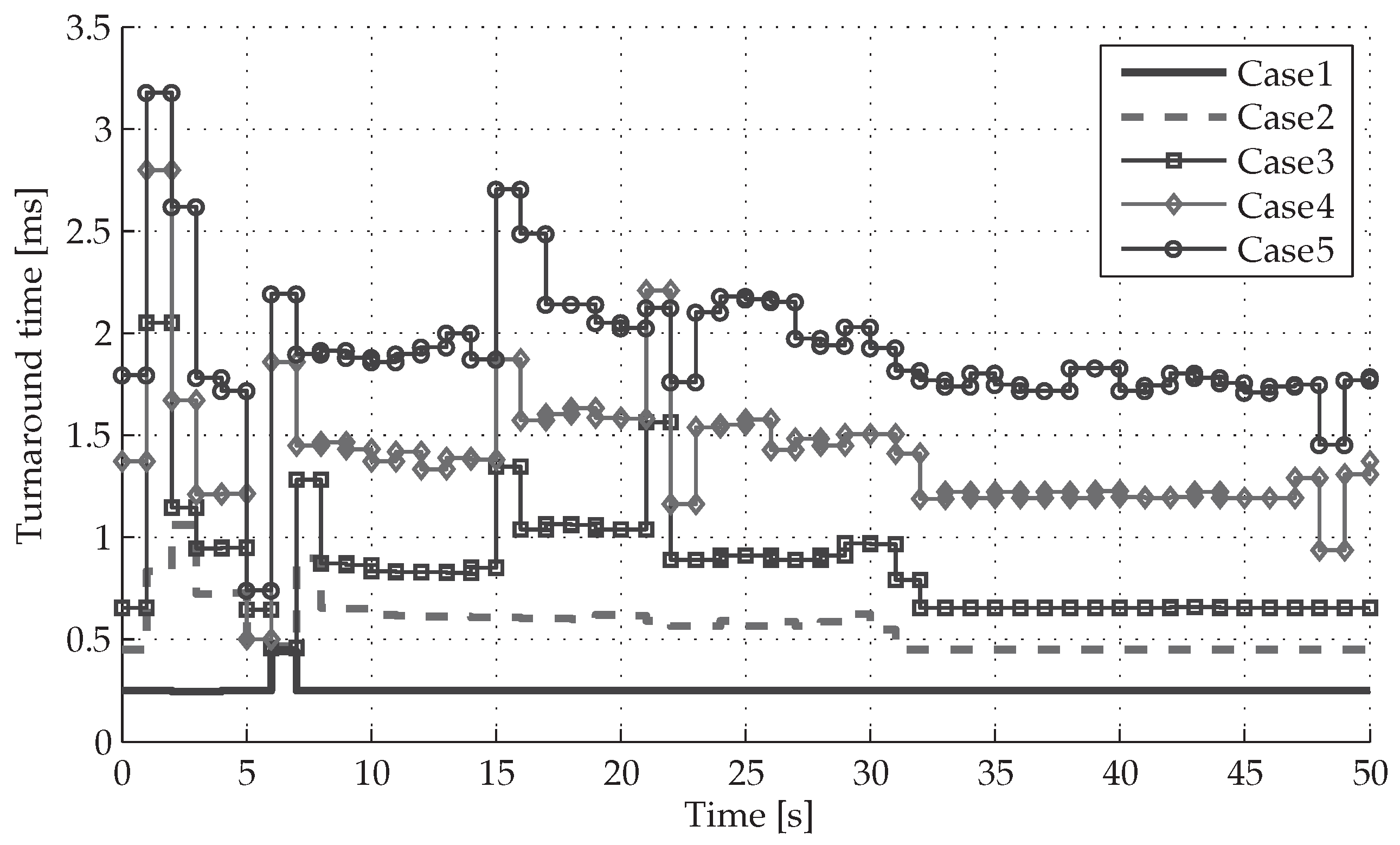
Five cases are given in Table 2 to analyze the scalability properties. The algorithm is running at 50 Hz and at each sampling period, one iteration of the dual decomposition algorithm is executed, i.e., the number of QPs as given in Table 2 are solved and the dual variables are updated once. This allows for 50 iterations as the setpoints for the subsystems are updated with a frequency of 1 Hz. The turnaround times of the algorithm are given in Figure 11 for each of the cases over the first 50 s of the drive cycle given in Figure 10. It is shown that by smart control of all subsystem (Case 5), the worst case execution time still only occupies 16% () of the sampling period. The remaining time can be used for other tasks or the update frequency of the setpoints can be lowered.
6. Conclusions
This paper proposes an online solution strategy for complete vehicle energy management. The approach is based on applying a dual decomposition to the receding horizon optimal control problem, so that the problem related to each subsystem can be solved separately. Each problem related to each subsystem is a linearly-constrained quadratic program that can be solved efficiently with embedded quadratic programming solvers. Variable prediction time intervals are used to obtain a long control horizon with a limited number of decision variables. As a result, the final state constraint can be used as a constraint, instead of a soft constraint. Furthermore, a novel on/off control concept for control of the refrigerated semi-trailer, the air supply system and the climate control system is introduced. The concept requires solving the linearly-constrained quadratic program twice, one with the first decision being on and one with the first decision being off. The solution with the lowest cost is taken as the optimal solution.
The proposed strategy requires limited tuning. Namely, the only parameters for the solution strategy proposed in this paper are the variable prediction time intervals and the penalty parameters for switching. The variable sample times can be chosen intuitively, and simulation results on a low-fidelity vehicle model show that close to optimal fuel reduction performance can be achieved without carefully tuning these sample times. The fuel reduction of the on/off controlled subsystems strongly depends on the number of switches allowed. The fuel reduction for the on/off controlled subsystems can be close to optimal, but the number of switches needs to increase significantly. Still, by allowing up to 15-times more switches, a fuel reduction of up to 1.3% can be achieved for the low-fidelity vehicle model with exact future knowledge of the disturbances.
The DEMPC approach has also been validated on a high-fidelity vehicle model, for which the propulsion power and the engine speed have been predicted by assuming that the vehicle follows a reference speed set by the cruise control or the downhill speed control, which is valid for highway driving. This allowed the vehicle speed to be predicted over a trajectory with a road slope predicted by an e-horizon sensor, e.g., ADASIS, leading to a prediction of the propulsion power and engine speed. The prediction algorithm has been validated with measured ADASIS information on a public road around Eindhoven, which demonstrated that accurate prediction of the propulsion power and engine speed is feasible if the vehicle follows the most probable path. A fuel reduction of up to 0.63% can be achieved for the high-fidelity vehicle model. This is indeed lower than estimated with the low-fidelity vehicle model, which can partly be related to the 25% less braking energy that is recovered in the high-fidelity vehicle model. Moreover, the absolute fuel consumption of the default control strategy is 10% higher. Therefore, future research should focus on methods for generating low-fidelity subsystem models from high-fidelity subsystem models, as well as allowing the DEMPC to control the hybrid power split, which is currently not possible in the high-fidelity model.
Acknowledgments
This work has received financial support from the FP7 of the European Commission under the grant CONVENIENT (312314). Furthermore, the authors would like to thank Wessel van Zon from DAF Trucks for providing the valuable ADASIS measurements used in this paper.
Author Contributions
Constantijn Romijn and Tijs Donkers developed the DEMPC algorithm. Constantijn Romijn simulated the approach and wrote the manuscript. Tijs Donkers, John Kessels and Siep Weiland reviewed and edited the manuscript. All authors read and approved the manuscript.
Conflicts of Interest
The authors declare no conflict of interest.
References
- Kessels, J.; Martens, J.; van den Bosch, P.; Hendrix, W. Smart vehicle powernet enabling complete vehicle energy management. In Proceedings of the 2012 IEEE Vehicle Power and Propulsion Conference, Seoul, Korea, 9–12 October 2012. [Google Scholar]
- De Jager, B.; van Keulen, T.; Kessels, J. Optimal Control of Hybrid Vehicles; Springer: London, UK, 2013. [Google Scholar]
- Guzzella, L.; Sciarretta, A. Vehicle Propulsion Systems; Springer: Berlin, Germany, 2007. [Google Scholar]
- Lin, C.C.; Peng, H.; Grizzle, J.W.; Kang, J.M. Power management strategy for a parallel hybrid electric truck. IEEE Trans. Control Syst. Technol. 2003, 11, 839–849. [Google Scholar]
- Ao, G.; Qiang, J.; Zhong, H.; Mao, X.; Yang, L.; Zhuo, B. Fuel economy and NOx emission potential investigation and trade-off of a hybrid electric vehicle based on dynamic programming. Proc. Inst. Mech. Eng. D J. Automob. Eng. 2008, 222, 1851–1864. [Google Scholar] [CrossRef]
- Pérez, L.V.; Bossio, G.R.; Moitre, D.; García, G.O. Optimization of power management in an hybrid electric vehicle using dynamic programming. Math. Comput. Simul. 2006, 73, 244–254. [Google Scholar] [CrossRef]
- Van Keulen, T.; Gillot, J.; de Jager, B.; Steinbuch, M. Solution for state constrained optimal control problems applied to power split control for hybrid vehicles. Automatica 2014, 50, 187–192. [Google Scholar] [CrossRef]
- Cipollone, R.; Sciarretta, A. Analysis of the potential performance of a combined hybrid vehicle with optimal supervisory control. In Proceedings of the IEEE International Conference on Control Applications, Munich, Germany, 4–6 October 2006. [Google Scholar]
- Serrao, L.; Rizzoni, G. Optimal control of power split for a hybrid electric refuse vehicle. In Proceedings of the IEEE American Control Conference, Seattle, WA, USA, 11–13 June 2008. [Google Scholar]
- Liu, C.; Liu, L. Optimal Power Source Sizing of Fuel Cell Hybrid Vehicles based on Pontryagin’s Minimum Principle. Int. J. Hydrogen Energy 2015, 40, 8454–8464. [Google Scholar] [CrossRef]
- Murgovski, N.; Johannesson, L.; Sjöberg, J.; Egardt, B. Component sizing of a plug-in hybrid electric powertrain via convex optimization. Mechatronics 2012, 22, 106–120. [Google Scholar] [CrossRef]
- Elbert, P.; Nüesch, T.; Ritter, A.; Murgovski, N.; Guzzella, L. Engine on/off control for the energy management of a serial hybrid electric bus via convex optimization. IEEE Trans. Veh. Technol. 2014, 63, 3549–3559. [Google Scholar] [CrossRef]
- Cikanek, S.; Bailey, K. Regenerative braking system for hybrid electric vehicles. In Proceedings of the IEEE American Control Conference, Anchorage, AK, USA, 8–10 May 2002. [Google Scholar]
- Hofman, T.; Steinbuch, M.; van Druten, R.; Serrarens, A. Rule-based energy management strategies for hybrid vehicles. Int. J. Electr. Hybrid Veh. 2007, 1, 71–94. [Google Scholar] [CrossRef]
- Serrao, L.; Onori, S.; Rizzoni, G. ECMS as a realization of Pontryagin’s minimum principle for HEV control. In Proceedings of the IEEE American Control Conference, St. Louis, MO, USA, 10–12 June 2009. [Google Scholar]
- Paganelli, G.; Ercole, G.; Brahma, A.; Guezennec, Y.; Rizzoni, G. General supervisory control policy for the energy optimization of charge-sustaining hybrid electric vehicles. JSAE Rev. 2001, 22, 511–518. [Google Scholar] [CrossRef]
- Paganelli, G.; Guerra, T.; Delprat, S.; Santin, J.; Delhom, M.; Combes, E. Simulation and assessment of power control strategies for a parallel hybrid car. Proc. Inst. Mech. Eng. D J. Automob. Eng. 2000, 214, 705–717. [Google Scholar] [CrossRef]
- Back, M.; Simons, M.; Kirschaum, F.; Krebs, V. Predictive control of drivetrains. IFAC Proc. Vol. 2002, 35, 241–246. [Google Scholar] [CrossRef]
- Kessels, J.; van den Bosch, P.; Koot, M.; de Jager, B. Energy management for vehicle power net with flexible electric load demand. In Proceedings of the IEEE Conference on Control Applications, Toronto, ON, Canada, 28–31 August 2005. [Google Scholar]
- Nuijten, E.; Koot, M.; Kessels, J.; de Jager, B.; Heemels, M.; Hendrix, W.; van den Bosch, P. Advanced energy management strategies for vehicle power nets. In Proceedings of the EAEC 9th International Congress: European Automotive Industry Driving Global Changes, Paris, France, 16–18 June 2003. [Google Scholar]
- Di Cairano, S.; Bernardini, D.; Bemporad, A.; Kolmanovsky, I.V. Stochastic MPC with learning for driver-predictive vehicle control and its application to HEV energy management. IEEE Trans. Control Syst. Technol. 2014, 22, 1018–1031. [Google Scholar] [CrossRef]
- Zeng, X.; Wang, J. A parallel hybrid electric vehicle energy management strategy using stochastic model predictive control with road grade preview. IEEE Trans. Control Syst. Technol. 2015, 23, 2416–2423. [Google Scholar] [CrossRef]
- Schepmann, S.; Vahidi, A. Heavy vehicle fuel economy improvement using ultracapacitor power assist and preview-based MPC energy management. In Proceedings of the 2011 American Control Conference, San Francisco, CA, USA, 29 June–1 July 2011. [Google Scholar]
- Borhan, H.; Vahidi, A.; Phillips, A.M.; Kuang, M.L.; Kolmanovsky, I.V.; Di Cairano, S. MPC-based energy management of a power-split hybrid electric vehicle. IEEE Trans. Control Syst. Technol. 2012, 20, 593–603. [Google Scholar] [CrossRef]
- Vahidi, A.; Greenwell, W. A decentralized model predictive control approach to power management of a fuel cell-ultracapacitor hybrid. In Proceedings of the IEEE American Control Conference, New York, NY, USA, 9–13 July 2007. [Google Scholar]
- Romijn, T.; Donkers, M.; Kessels, J.; Weiland, S. A Distributed Optimization Approach for Complete Vehicle Energy Management. Trans. Control Syst. Technol. 2017. submitted. [Google Scholar]
- Chen, H. Game-Theoretic Solution Concept for Complete Vehicle Energy Management. Ph.D. Thesis, Technische Universiteit Eindhoven, Eindhoven, The Netherlands, 2016. [Google Scholar]
- Nguyen, K.D.; Bideaux, E.; Pham, M.T.; Le Brusq, P. Game theoretic approach for electrified auxiliary management in high voltage network of HEV/PHEV. In Proceedings of the IEEE International Electric Vehicle Conference, Florence, Italy, 17–19 December 2014. [Google Scholar]
- Nilsson, M.; Johannesson, L.; Askerdal, M. ADMM applied to energy management of ancillary systems in trucks. In Proceedings of the IEEE American Control Conference, Chicago, IL, USA, 1–3 July 2015. [Google Scholar]
- Ellis, M.; Durand, H.; Christofides, P.D. A tutorial review of economic model predictive control methods. J. Process Control 2014, 24, 1156–1178. [Google Scholar] [CrossRef]
- Albalawi, F.; Durand, H.; Christofides, P.D. Distributed economic model predictive control for operational safety of nonlinear processes. AIChE J. 2017. [Google Scholar] [CrossRef]
- Chen, X.; Heidarinejad, M.; Liu, J.; Christofides, P.D. Distributed economic MPC: Application to a nonlinear chemical process network. J. Process Control 2012, 22, 689–699. [Google Scholar] [CrossRef]
- Romijn, T.; Donkers, M.; Kessels, J.; Weiland, S. Receding Horizon Control for Distributed Energy Management of a Hybrid Truck with Auxiliaries. In Proceedings of the IFAC Workshop on Engine and Powertrain Control, Simulation and Modeling, Columbus, OH, USA, 23–26 August 2015. [Google Scholar]
- Khalik, Z.; Romijn, T.; Donkers, M.; Weiland, S. Effects of battery charge acceptance and battery aging in complete vehicle energy management. In Proceedings of the IFAC World Congress, Toulouse, France, 9–14 July 2017. [Google Scholar]
- Van der Sanden, N. Model Identification of DAFs EURO-6 Air-Conditioning System Applied in an Optimal Control Study. Master’s Thesis, Eindhoven University of Technology, Eindhoven, The Netherlands, 2014. [Google Scholar]
- Cagienard, R.; Grieder, P.; Kerrigan, E.C.; Morari, M. Move blocking strategies in receding horizon control. J. Process Control 2007, 17, 563–570. [Google Scholar] [CrossRef] [Green Version]
- Mattingley, J.; Boyd, S. CVXGEN: A code generator for embedded convex optimization. Optim. Eng. 2012, 13, 1–27. [Google Scholar] [CrossRef]
- Ferreau, H.; Kirches, C.; Potschka, A.; Bock, H.; Diehl, M. qpOASES: A parametric active-set algorithm for quadratic programming. Math. Program. Comput. 2014, 6, 327–363. [Google Scholar] [CrossRef]
- Lingman, P.; Schmidtbauer, B. Road slope and vehicle mass estimation using Kalman filtering. Veh. Syst. Dyn. 2002, 37, 12–23. [Google Scholar] [CrossRef]
- Winstead, V.; Kolmanovsky, I.V. Estimation of road grade and vehicle mass via model predictive control. In Proceedings of the IEEE Conference on Control Applications, Toronto, ON, Canada, 28–31 August 2005. [Google Scholar]
- Vahidi, A.; Stefanopoulou, A.; Peng, H. Experiments for online estimation of heavy vehicles mass and time-varying road grade. In Proceedings of the ASME International Mechanical Engineering Congress and Exposition, Washington, DC, USA, 15–21 November 2003. [Google Scholar]
- Fathy, H.K.; Kang, D.; Stein, J.L. Online vehicle mass estimation using recursive least squares and supervisory data extraction. In Proceedings of the American Control Conference, Seattle, WA, USA, 11–13 June 2008. [Google Scholar]
- Ress, C.; Balzer, D.; Bracht, A.; Durekovic, S.; Löwenau, J. Adasis protocol for advanced in-vehicle applications. In Proceedings of the 5th World Congress on Intelligent Transport Systems, New York, NY, USA, 16–20 November 2008. [Google Scholar]
- Chen, H.; Kessels, J.; Weiland, S. Vehicle energy management for on/off controlled auxiliaries: Fuel economy vs. Proceedings switching frequency. In Proceedings of the IFAC Workshop on Engine and Powertrain Control, Simulation and Modeling, Columbus, OH, USA, 23–26 August 2015. [Google Scholar]
- Bertsekas, D.P. Dynamic Programming and Optimal Control; Athena Scientific: Belmont, MA, USA, 1995; Volume 1. [Google Scholar]
- Eckstein, L.; Mohrmann, B.; Hummel, R.; Weiland, S.; Donkers, M.; Chen, H.; Romijn, T. Fuel consumption reduction measures for longhaul-trucks in the CONVENIENT project. In Proceedings of the 13th International Conference Commercial Vehicles, Eindhoven, The Netherlands, 10–11 June 2015. [Google Scholar]
- Mohrmann, B.; Hummel, R.; Gissing, J.; Kessels, J. Holistic Energy System Design; Technical Report, Convenient Project Deliverable Report D A3.2.1; IKA: Aachen, Germany, 2014. [Google Scholar]
Figure 1.
Topology of a hybrid truck with high-voltage and low-voltage auxiliaries and where the arrows indicate the direction of a positive power flow.
Figure 1.
Topology of a hybrid truck with high-voltage and low-voltage auxiliaries and where the arrows indicate the direction of a positive power flow.

Figure 2.
Power losses of the internal combustion engine, the electric machine and the alternator for two different engine speeds.
Figure 2.
Power losses of the internal combustion engine, the electric machine and the alternator for two different engine speeds.

Figure 3.
Prediction of at some future time .

Figure 4.
Part 1 () and Part 2 () of a PAN European driving cycle.
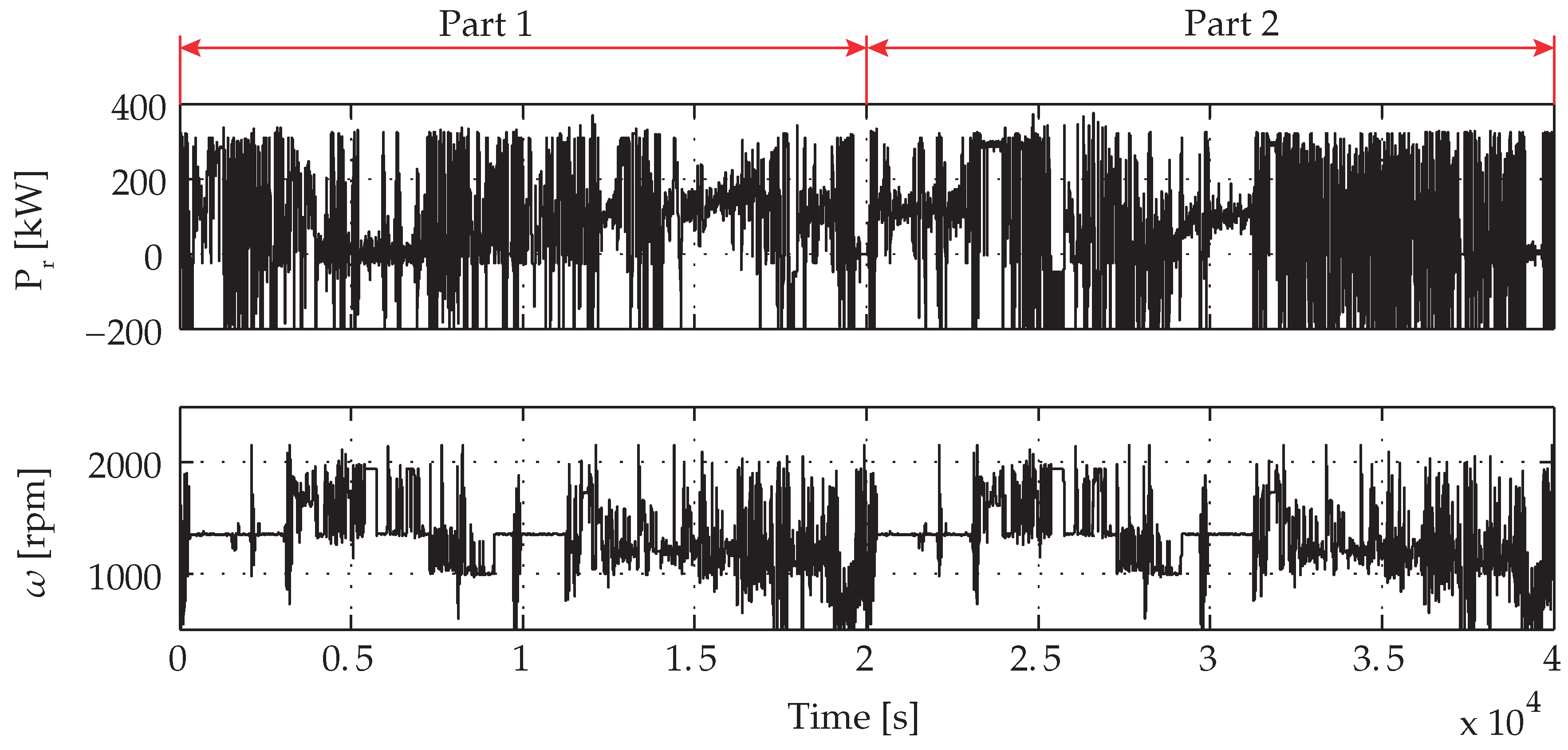
Figure 5.
Fuel reduction of a hybrid heavy-duty vehicle for two parts of the drive cycle and various cases. (a) Part 1; (b) Part 2.
Figure 5.
Fuel reduction of a hybrid heavy-duty vehicle for two parts of the drive cycle and various cases. (a) Part 1; (b) Part 2.
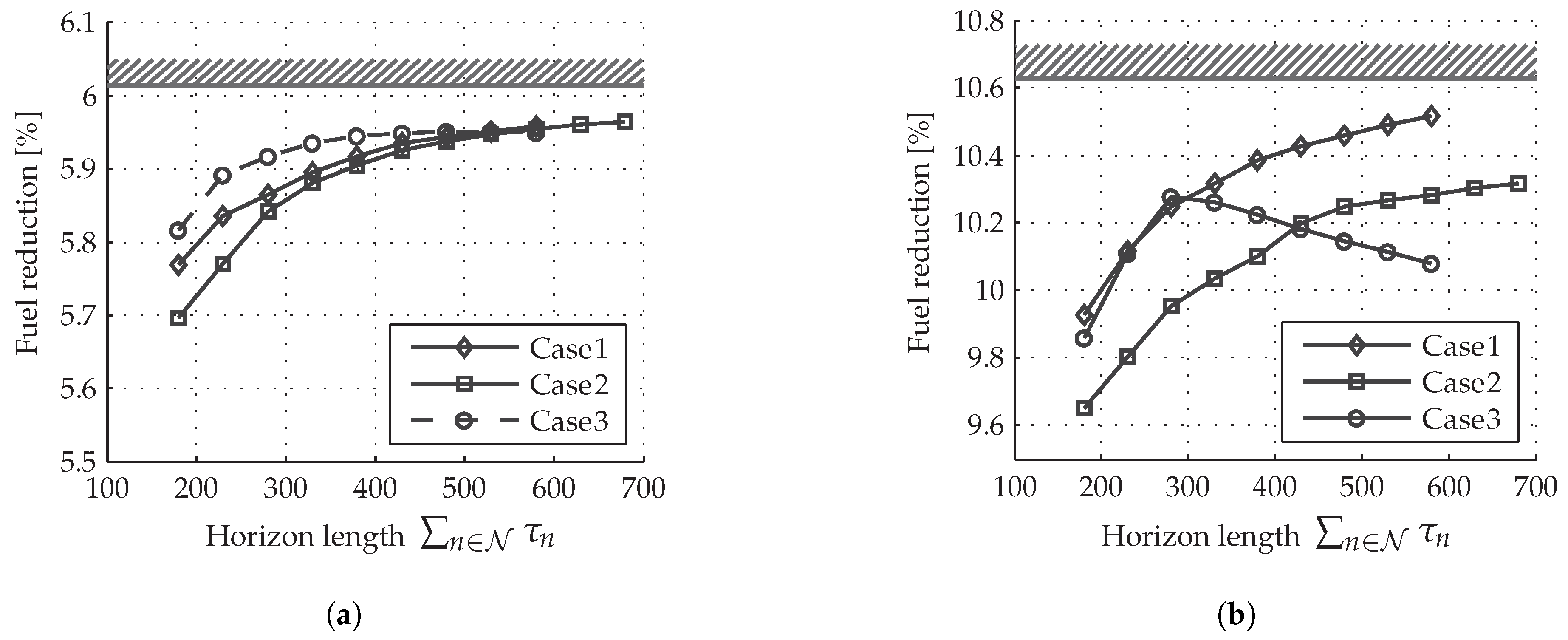
Figure 6.
Sensitivity to the pre-specified value of . (a) Part 1; (b) Part 2.
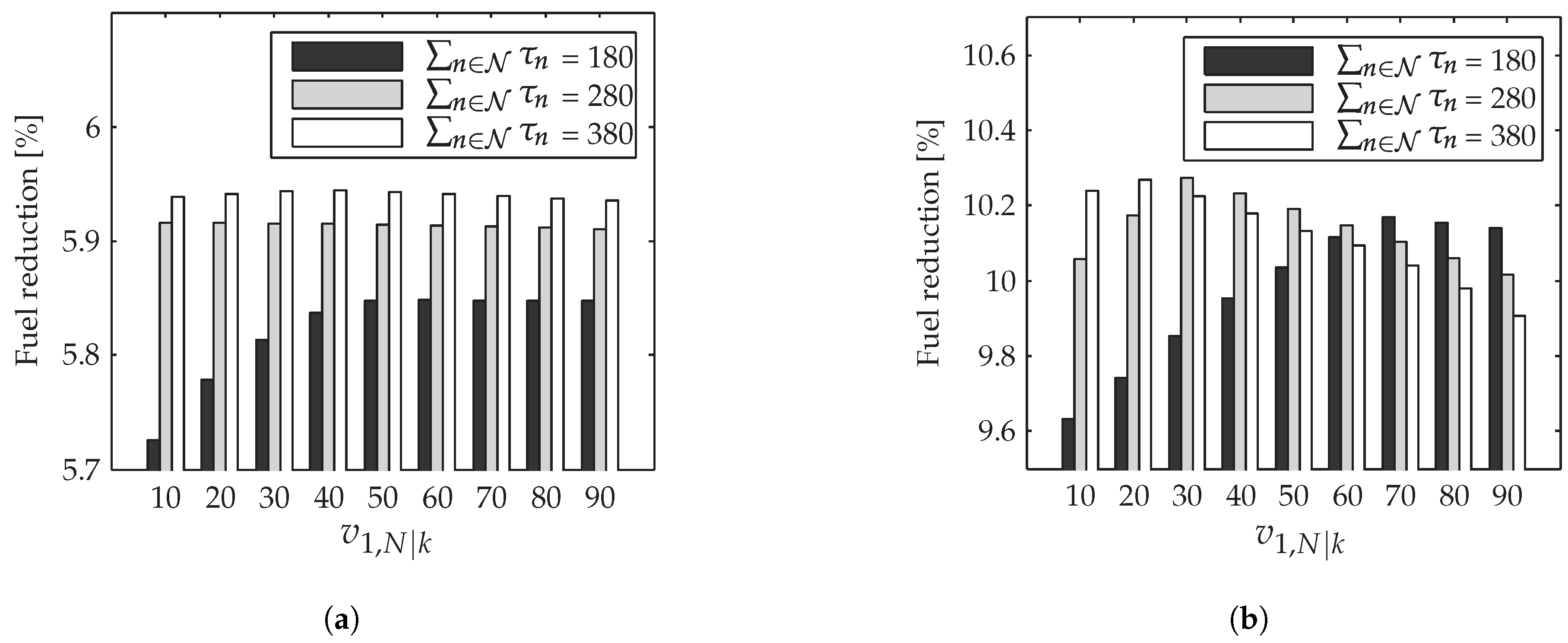
Figure 7.
Fuel reduction with real-time on/off control of the refrigerated semi-trailer, the air supply system and the climate control system for three different switching strategies. (a) Refrigerated semi-trailer, Part 1; (b) Refrigerated semi-trailer, Part 2; (c) Air supply system, Part 1; (d) Air supply system, Part 2; (e) Climate control system, part 1; (f) Climate control system, Part 2.
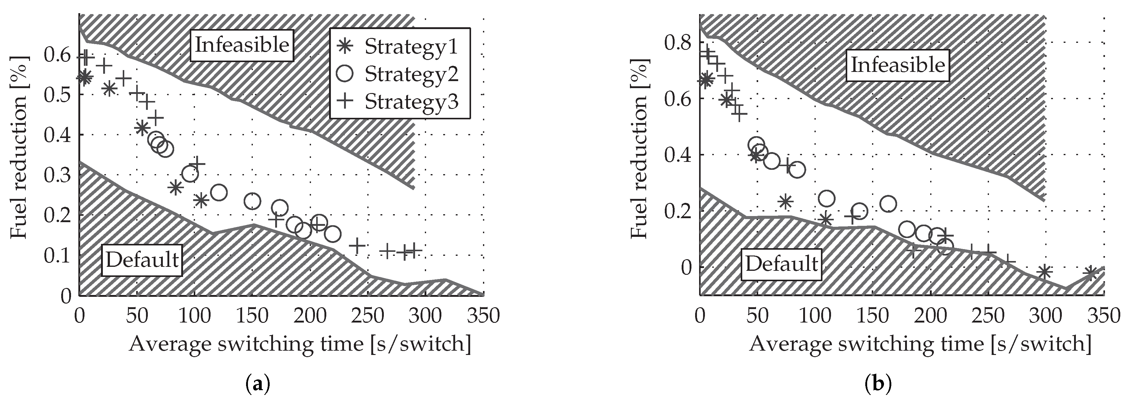

Figure 8.
Fuel reduction as a result of smart control of auxiliaries with number of iterations being limited. (a) Part 1; (b) Part 2.
Figure 8.
Fuel reduction as a result of smart control of auxiliaries with number of iterations being limited. (a) Part 1; (b) Part 2.

Figure 9.
High-fidelity vehicle model.

Figure 10.
Road load prediction with Algorithm 2 and ADASIS.

Figure 11.
Turnaround times.

Table 1.
Fuel reduction results on the high-fidelity vehicle model. CVEM, complete vehicle energy management.
Table 1.
Fuel reduction results on the high-fidelity vehicle model. CVEM, complete vehicle energy management.
| Subsystem | Fuel Reduction | |
|---|---|---|
| Part 1 | Part 2 | |
| Refrigerated semi-trailer | ||
| Air supply system | ||
| Climate control system | 0% | |
| Alternator | ||
| DCDC converter | ||
| CVEM | ||
Table 2.
Case studies for real-time control. QP, quadratic program.
| Case | Description | No. of QPs at Each Iteration |
|---|---|---|
| 1 | Only hybrid system | 1 |
| 2 | Case 2 with smart RST | 3 |
| 3 | Case 3 with smart AS | 5 |
| 4 | Case 3 with smart HVAC | 7 |
| 5 | All smart | 8 |
© 2017 by the authors. Licensee MDPI, Basel, Switzerland. This article is an open access article distributed under the terms and conditions of the Creative Commons Attribution (CC BY) license (http://creativecommons.org/licenses/by/4.0/).
Share and Cite
MDPI and ACS Style
Romijn, C.; Donkers, T.; Kessels, J.; Weiland, S. Real-Time Distributed Economic Model Predictive Control for Complete Vehicle Energy Management. Energies 2017, 10, 1096. https://doi.org/10.3390/en10081096
AMA Style
Romijn C, Donkers T, Kessels J, Weiland S. Real-Time Distributed Economic Model Predictive Control for Complete Vehicle Energy Management. Energies. 2017; 10(8):1096. https://doi.org/10.3390/en10081096
Chicago/Turabian StyleRomijn, Constantijn, Tijs Donkers, John Kessels, and Siep Weiland. 2017. "Real-Time Distributed Economic Model Predictive Control for Complete Vehicle Energy Management" Energies 10, no. 8: 1096. https://doi.org/10.3390/en10081096
Note that from the first issue of 2016, this journal uses article numbers instead of page numbers. See further details here.