A Large Scale Grid Data Analysis Platform for DSOs


1
Center for Energy - Electric Energy Systems, AIT Austrian Institute of Technology, Vienna 1210, Austria
2
Institute of Energy Systems and Electrical Drives, TU Wien, Vienna 1040, Austria
*
Author to whom correspondence should be addressed.
Energies 2017, 10(8), 1099; https://doi.org/10.3390/en10081099
Submission received: 7 June 2017
/
Revised: 14 July 2017
/
Accepted: 14 July 2017
/
Published: 27 July 2017
Abstract
:The number of fluctuating distributed energy resources (DER) in electricity grids is continuously rising. Due to the lack of operational information on low-voltage (LV) networks, conservative assumptions are necessary to assess the connection of generators to the grid. This paper introduces the hosting capability (HC) as a measure to assess the amount of DER that can be integrated in LV-feeders. The HC of a feeder is the minimum amount of DER that can be hosted in a feeder without reinforcement needs for a given DER-scenario and for a given admissible voltage rise. The hosting capability assessment was performed on the entire LV-grid data of two Austrian Distribution System Operators (DSOs) with more than 36,000 LV-feeders. In total, 40 HC-scenarios were calculated with varying admissible voltage rise levels, DER-scenarios and reactive power control strategies. It turned out that only few feeder parameters such as the resistance at the end node and the lowest ampacity value of feeders show a high correlation with the calculated HC. Further, the impact of the DER-scenario on the share of voltage and loading constrained feeders is rather limited. The gathered results are suitable to validate equivalent LV-feeders models to perform integrated power flow studies on the transmission and distribution grids. Besides the results obtained for the network data of the two DSOs, a performant, modular and parallelizable tool has been developed to automatically analyze large LV network sets.
1. Introduction
In the last decades, the installed capacity of distributed energy resources (DER) increased rapidly [1]. Distribution networks, initially planned to supply customers, are now connecting a large number of DER which leads to voltage rise and loading constraints [2]. In [3], PV was stated to be in the two most installed sources of electricity in the European Union in 2013.
In [4], it is reported that solar PV is already covering more than 7% of the electricity demand in three countries (Italy, Greece and Germany). Further, in 2014, the power generation capacities for Wind and solar PV in the EU 28 increased by 11,791 MW and 6574 MW, respectively. Globally, about 40 GW solar PV have been installed in 2014. Moreover, the total amount of installed Solar Power in the world reached 178 GW and covers more than 1% of the world electricity demand.
However, to reduce CO2 emission even more renewable energy resources are required [5,6,7,8]. Acknowledging the challenges for distribution grids, efforts are needed to limit investments in network reinforcements required to integrate the expected amount of DER.
The detailed investigation of the hosting capacity of the entire supply of a DSO may be a computationally burden. In [9] the LV-grid data of the largest Dutch DSO is classified. This DSO operates about 88,000 LV-feeders and authors report, that the individual analysis of all LV-feeders is enormously time consuming. In [10] for example, only 1.35% of the grid data of a DSO was analyzed and three main feeder topologies were presented. This issue can be solved in several ways. First, a common approach in the literature is to cluster networks and focus on representative networks of each cluster. Results are then scaled up for the entire supply area. Several reference networks were defined in the past. For example, in [11], representative networks were defined for Bavaria based on real network data and this set of representative networks were updated in [12]. In [13] it was shown that clustering of distribution networks by means of electrical/topological indices can be reduced to several relevant parameters and a criterion to define a reasonable number of clusters is given. In [14], a Matlab GUI is presented, which generates statistically correct distribution grid models. Authors point out that such generators are crucial for new applications development such as monitoring and control.
Third, calculations can be distributed to several machines or cores. In [15], the issue that network calculation tools mostly run on single core architectures running calculations sequentially is addressed. For this reason a very promising high performance computation framework called GridPACK (Battelle Memorial Institute, Columbus, OH, USA) was developed. For a 156-bus system and 1024 contingencies, the overall solution time could be reduced from 2 h to less than a minute.
The second approach to reduce computation time is to restrict the number of nodes in a power flow calculation. According to [16], low voltage networks can be reduced to a two-bus equivalent model for pre-screening of large supply areas to identify networks where more likely voltage violations may occur. Moreover, “continuous feeders” are used for studies on specific inverter functionalities to control the voltage [17]. In [18], benchmark feeders are proposed using a similar approach.
Generic networks have received attention for benchmarking in the frame of specific DSO-revenue regulations. Thereby, tools and methods known from graph theory such as the minimum spanning tree may be suitable for the benchmark of distribution grids. In [19], the Prize-Collecting Steiner Tree algorithm is utilized to connect customers (e.g., optic fiber, district heating sector) cost-efficiently to the network. Moreover, in [20,21], the Facility Location Problem is applied to LV-networks to assist network planners and operators to optimally place secondary substations. In [22], the “betweenness” is used as a measure to identify vulnerable lines according to either topological point of view or by considering the actual power flows.
In [23], Kendall’s correlation was used to reduce redundancy between input parameters. Among 13 input parameters, the total cable length of feeders, the share of cables and aerial lines, connection points per length, the yearly consumption and the installed capacity of PV-systems were identified as most important parameters. In [24], distribution grids of western Australia are classified and prototypical feeders are selected at both MV and LV-level. On LV-level, 26 parameters were investigated, such as secondary transformer rating, feeder length, energy consumption (for residential, commercial and industrial respectively), number of customers and many more. The identified most significant seven parameters are similar to previously mentioned studies: underground cable length, load capacity of residential customers, number of residential customers, overhead-line length and others. The cluster analysis on LV feeder level resulted in an optimal cluster number of eight and a description of the LV feeder subsets is given.
This paper presents findings from an environment that is capable of analyzing a high number of networks and performing various in-depth studies. During the project IGREENGrid ((IntegratinG Renewables in the EuropEaN Electricity Grid) [25], the complete distribution grid data of two Austrian DSOs with more than 14,000 LV-networks were provided from their GIS systems and imported into PowerFactory (DIgSILENT, Gomaringen, Baden-Württemberg, Germany) [26]. Thereby, the provided data by the DSOs had a different format. In the case of DSO A, the network data stored in a GIS database were exported in the DIgSILENT DGS format. In the case of DSO B, the data were provided from the GIS database as Neplan export (*.cde, *.edt, and *.ndt files). In Figure 1, the import process, which was automated with the DIgSILENT Programming Language (DPL) is depicted. In total about 14,600 networks with approximately 54,100 feeders were imported. For about 41,000 feeders, load flow and short circuit calculations were performed. After a plausibility check, more than 36,000 feeders were assessed.
A high number of feeder parameters such as the number of load, number of nodes, average distance to neighboring nodes, average number of nodes, equivalent sum impedance, ampacity of lines, feeder length, etc. were investigated. The hosting capability (HC) of LV-feeders was investigated considering reactive power control strategies and several DER-scenarios for a high number of voltage limits. Based on these results, feeders can be classified according to the limiting constraint (voltage or loading). Further, a sensitivity analysis of the limiting constraint on the admissible voltage rise is performed. Additionally, parameters of feeders are investigated and probability tests for selected parameters are performed. This analysis is supplemented by a linear (Pearson) and a rank (Spearman) correlation analysis of feeder parameters and admissible DER penetration levels according to the considered scenarios.
Based on these results, the impact of the DER-scenario on the constraint reason is evaluated. Moreover, suggestions to either increase the admissible voltage band or apply a reactive power control strategy to integrate a higher number of DER are given. Furthermore, for the grid data of one investigated DSO whether the minimal spanning tree is a suitable tool to benchmark DSOs is analyzed.
The paper is organized as follows: First the Materials and Methods are described in Section 2. Results on feeder classification and high-level indicators are presented in Section 3. In Section 4 a comprehensive study on the DER-scenarios and reactive power control strategies is given. In Section 5, the correlation between feeder parameters and the HC is investigated. The paper is concluded in Section 6.
2. Materials and Methods
In this section, the hosting capability (HC) is introduced, followed by scenario definitions regarding the DER-distribution, reactive power control strategy and admissible voltage rise. After that, the two most important constraints limiting the HC are discussed. Next, the assessed feeder parameters and the algorithms to perform the simulation are presented. Finally, two benchmarking measures are presented.
In this work, the amount of DER that can be hosted in LV-feeders is investigated. For that, the hosting capability is defined:
“The hosting capability of a LV-feeder is the amount of DER that can be installed for a given DER-scenario while meeting voltage and loading prerequisites in the feeder.” The hosting capacity evaluation considers as system boundary the LV feeders (not considering the distribution transformer). Moreover, loads are not explicitly taken into account (see the justification below) and further factors that might limit the hosting capacity such as the impact on protection schemes are not considered here (considered as secondary factors).
Load assumptions have in general a high impact on the achievable HC. In [27], it is reported that “The worst cases of voltage rise occur when the PV-DG is at or close to its maximum output, and the difference between the load and the generation is at its highest” and further “Using deterministic models with average values for the loads underestimates the voltage impact of increasing PV-DG because the real loads on a feeder vary”. Generally, the base load can be well monitored at secondary transformers supplying a particular area with a high number of customers. These customers are usually supplied by more than one feeder. However, given the small number of loads and generators connected to a single LV feeder, the existence of a certain base load level may not be given permanently at particular nodes in the feeder. In [28], a stochastic analysis was performed on the smart meter data of 1077 customers (households and PV generators) measured over a period of one year. Authors evaluated the peak and average load depending on the number of households in the respected area that needs to be considered in network planning. For a feeder with five households a significantly higher peak load (15 kW) and lower base load (0.5 kW) compared to 100 households (200 kW, 22 kW respectively) has to be considered. These values are measured at the beginning of the feeder. Therefore, reasonable base load assumptions could not be defined at specific nodes (e.g., end node). The simultaneity factor for the balanced PV infeed as well as the orientation and tilt is assumed to be identical for all generators (worst case). Under these conditions, the hosting capability of a feeder heavily depends on the location of the generation along the feeder as well as on the allowed voltage rise and loading limit of lines.
A high penetration level of DER in distribution grids may lead to protection issues that need to be avoided. Authors in [29] conclude that the fault devices need to handle the additional fault current by DER and that for fuse-fuse coordination a higher fault current by DER is beneficial, while for the fuse-recloser coordination DER the fault injection should be minimal. In [30], it is stated that with the increasing DER penetration, the radial structure of distribution feeders will be changed to a meshed configuration. Further, a methodology is proposed to determine the size of DG sources while the existing protection scheme can be maintained. Authors in [31] point out that a large-scale penetration of DER may lead to protection blinding and sympathetic tripping and other failures in meshed MV-grids. However, to which extent these issues can be translated to radial LV-feeders, requires further investigations.
According to the hosting capability definition, the remaining constraint that could be violated is that the total hosting capability of all feeders may exceed the rating of the secondary transformer supplying these feeders. However, whether this issue arises depends on several circumstances:
- Could the full hosting capability potential be utilized (e.g., available DER roof-top potential)?
- Which time frame can be expected for the full deployment of DER?
- What is the actual minimal load at the transformer and expected growth of consumption?
- Are network topology changes foreseen (additional feeders, feeders supplied by other secondary substations)?
Hence, there are remaining reserves regarding the full deployment of the hosting capability of all LV-feeders supplied by a secondary substation.
Three DER scenarios were considered (Figure 2 left):
- “Uniform”: Generation resources placed uniformly along the feeder (at all connection boxes) and then scaled-up to reach the hosting capability (loading limit or voltage limit is reached).
- “Weighted”: Generation resources distributed according to the summed annual consumption at the connection boxes) and then scaled-up to reach the hosting capability. This scenario is relevant when assuming that in the future most of DER deployment will be close to the loads and driven by self-consumption.
- “End of feeder” (eof): Generation resources connected at the “end node” which is defined as the node with the highest voltage for the uniform scenario (this scenario can be considered as “worst-case”).
Beside the DER scenarios, different reactive power control concepts have been considered (Figure 2 middle): a fixed PF = 0.9 and Q(U)-control. For the Q(U)-control, a minimal PF of 0.9 is allowed. Furthermore, voltage regulated distribution transformer VRDT (transformer with On-Load-Tap-Changer (OLTC)) are considered in this study since they lead to an increase of the hosting capacity by decoupling medium and low voltage networks. This decoupling allows using a larger share of the voltage band for the LV network than the share currently allocated (without VRDT). Hence, a voltage rise of up to 8% of the nominal voltage (Figure 2 right) may be admissible.
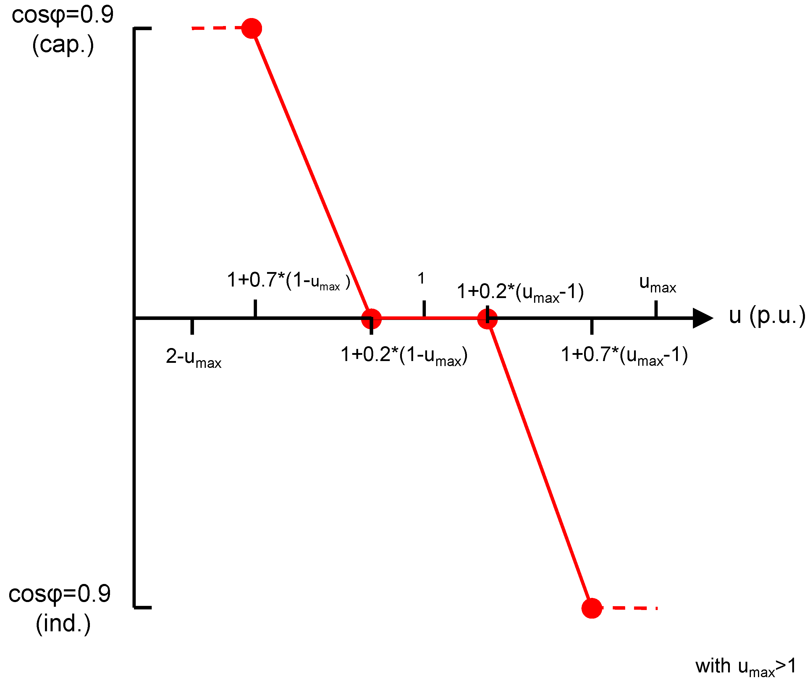
The considered Q(U) control is depicted in Figure 3 and consists of a dead band, droop and a saturation area for over and under voltage. Thereby the set points of the Q(U)-control are configured according to the admissible voltage rise. For the dead band, 20% of the voltage band is allocated, while for the saturation area 30% is reserved. The remaining voltage band is dedicated to the droop control.
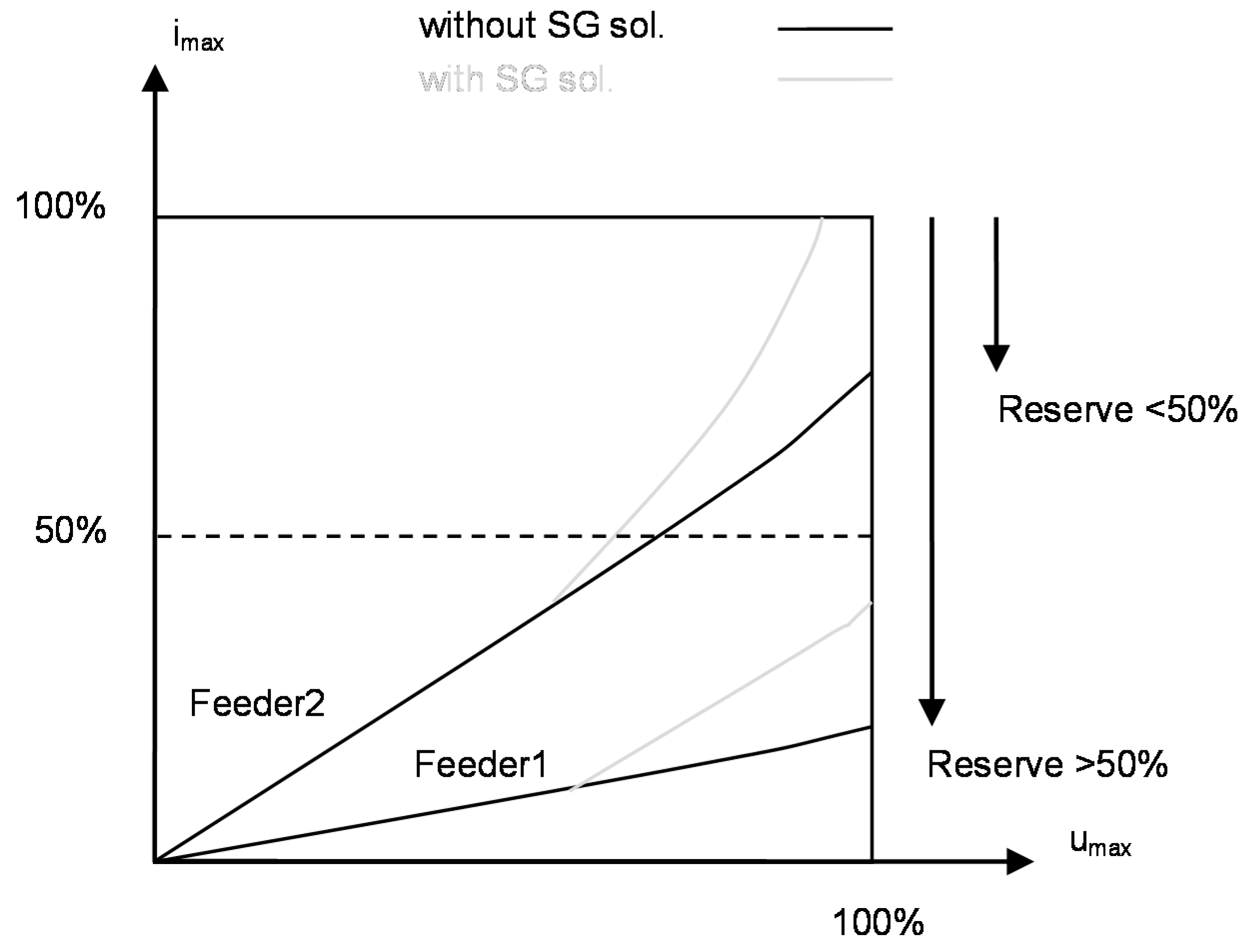
The concept of hosting capacity introduced in [32] is restricted to the two most relevant limitations in distribution networks: the maximal admissible voltage rise and the maximal admissible loading. An illustration of this is shown in Figure 4. If the hosting capacity of a voltage constrained feeder is increased by means of reactive power control, the loading reserve is reduced (Feeder 1). However, if the loading reserve is rather small, as in the case of Feeder 2, the full potential of reactive power control strategies cannot be deployed since the feeder would be overloaded by the additional reactive power flow.
The problem formulation for the optimization of the HC of a feeder is given in Equation (1), where f is a feeder of Network N, ui the voltage at bus i, lj the loading of line j of the feeder. The admissible loading Lmax of lines is defined as 100% of the respective nominal current. The voltage limit umax is determined by the investigated scenario (1.01 to 1.08 p.u.).
Based on the assumption in Figure 2 and the problem formulation in Equation (1), the HC is obtained with an adapted Newton–Raphson (NR) algorithm to reach one of the two constraints depicted in Figure 4 (voltage or loading). For that, two NR-optimizations are performed to calculate the highest HC without violating the admissible voltage rise and the loading of network elements (Figure 5). In each step, the lower estimated HC is selected for the next iteration.
By means of active power curtailment (P(U)-control), the HC could be increased even further. However, the objective is to maximize the HC of feeders according to the DER-distribution. A P(U)-control would curtail the injected power unequally, since the power would in tendency be more curtailed at the most distant installation where the highest voltage rise occurs. This would cause varying injected powers for the DER-scenario uniform. Hence, considering a P(U)-control in the optimization of the HC would lead to a contradiction that cannot be resolved while maximizing the injected power for all generators in the feeder in a fair way. The amount of curtailed energy however depends on several other factors such as location, connection point, orientation and tilt of the installation, load behavior, etc.
Parameters used for classification in [11,33] are considered as well as several other parameters are investigated, which might be suitable to estimate the HC without power flow calculations. Table 1 gives an overview on investigated parameters. Parameters used in literature to classify networks are underlined. A key design element of the platform is that the data analysis runs on feeder level. This allows incomplete data leading only to the exclusion of affected feeders, while remaining feeders in the same network are processed. Some parameters are suitable to check the plausibility of the feeder data. Parameters listed to validate the classification are available for validation purposes. However, these parameters are listed by benefits, e.g., a classification to estimate the hosting capability has the highest benefits. The equivalent load location is the node in the feeder, where the total load has to be placed to cause a similar voltage drop compared to the initial situation. The aggregated obtained hosting capability of feeders may exceed the nominal rating of the secondary transformer. Therefore, the transformer data are also assessed in the static analysis.
The formulas for not evident parameters are given in Equations (2)–(7), where N is the number of Nodes in the feeder.
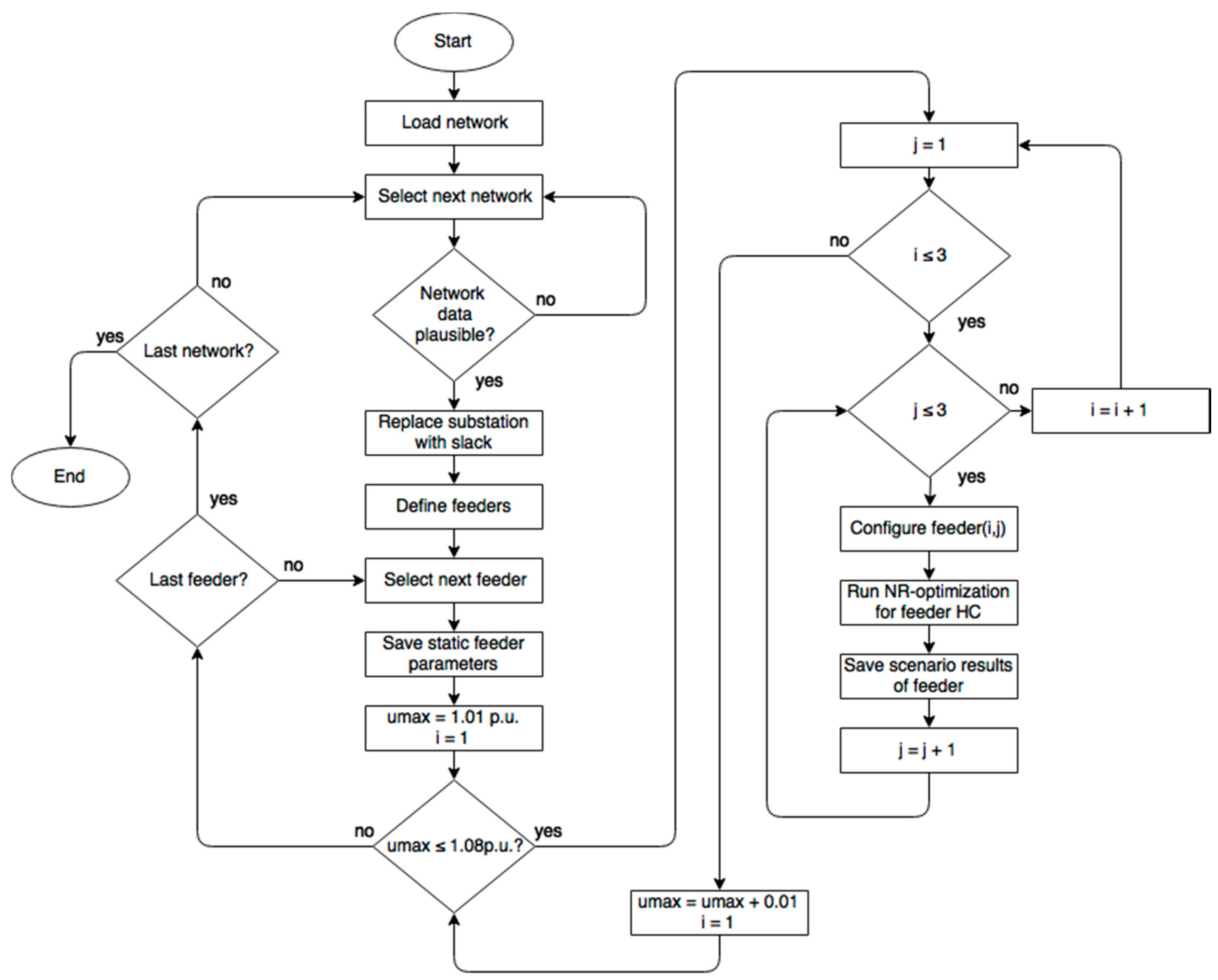
In Figure 6, the implemented algorithm is depicted. Each network is assessed for given input parameters (Voltage Limits, control strategies and DER distribution). After a plausibility test, feeders are defined and the secondary substation of the networks is replaced by a LV slack node. Omitting the transformer allows to study only feeder relevant parameters and avoid mischaracterization of identical feeders caused by different secondary transformers types. First, for each feeder, parameters that are invariant of any assumptions are calculated (static parameters such as the feeder length, ZK and ZΣ). Parameters such as the ZK or Inom can be used to check the plausibility of network data (incomplete or corrupt). Next, the HC for each scenario according to Figure 2 is calculated and parameters based on these assumptions are obtained (scenario results). Thereby, i defines the control strategy (uncontrolled, cosϕ = 0.9, VoltVAr) and j the DER-scenario (uniform, eof, and weighted). For each scenario, the NR-algorithm is utilized to obtain the maximal HC under the given voltage (umax) constraint without overloading any network element.
The algorithm is designed to export one file per network and the combination of voltage limit, control strategy, distribution scenario as well as one file per parameter group (static feeder data, parameters requiring a power flow or short-circuit calculation, etc.). In the current configuration, there are 85 files per network available for analysis (Figure 7). Hence, this allows running or repeating parts of the study in a modular way. Therefore, two ways of parallelizing the computation to reduce the running time are possible: distributing the grid data or running specific scenarios for the same networks on several machines.
The running time for all presented scenarios in Figure 6, for 14,600 networks of two DSOs depends on the number of available cores and machines. For each feeder in the networks a NR-optimization with several iterations is performed to calculate the HC according to the scenarios. Running on a single core on a single machine (worst case) e.g., on a standard laptop with an Intel® Core™ i7-2640M @2.8Ghz processor (Intel, Santa Clara, CA, USA), about 40–45 networks can be processed per hour (networks have on average 4.4 feeders and feeders have on average 22 nodes). For each scenario and feeder, several contingencies are calculated with the presented NR-optimization to obtain the maximal HC.
Some regulatory concepts require the comparison of different DSOs across the country to benchmark the capital expenditure (CAPEX) and operational expenditure (OPEX). For example, the weighted transformed connection density (trfNAD) is used as one component to compare DSO in the benchmarking process [34] in Austria. Equation (8) shows a simplified version of this parameter, where A is the supplied area and N is the number of connection points in the considered area.
3. Advanced Tool for Automatic Feeder Analysis and Characterization
In this section, the results on feeder characterization are presented followed by the evaluation of high-level indicators to compare networks.
3.1. Results on Feeder Characterization
In this section, the results on feeder characterization are summarized. Based on the methodology in [35], 40 hosting capability values were calculated (DER-scenario/voltage limit/control strategy) and classified as voltage/loading constrained. Further, the effect of DER scenarios on the characterization is analyzed. Finally, the hosting capability values are correlated with parameters that are used in literature for network clustering.
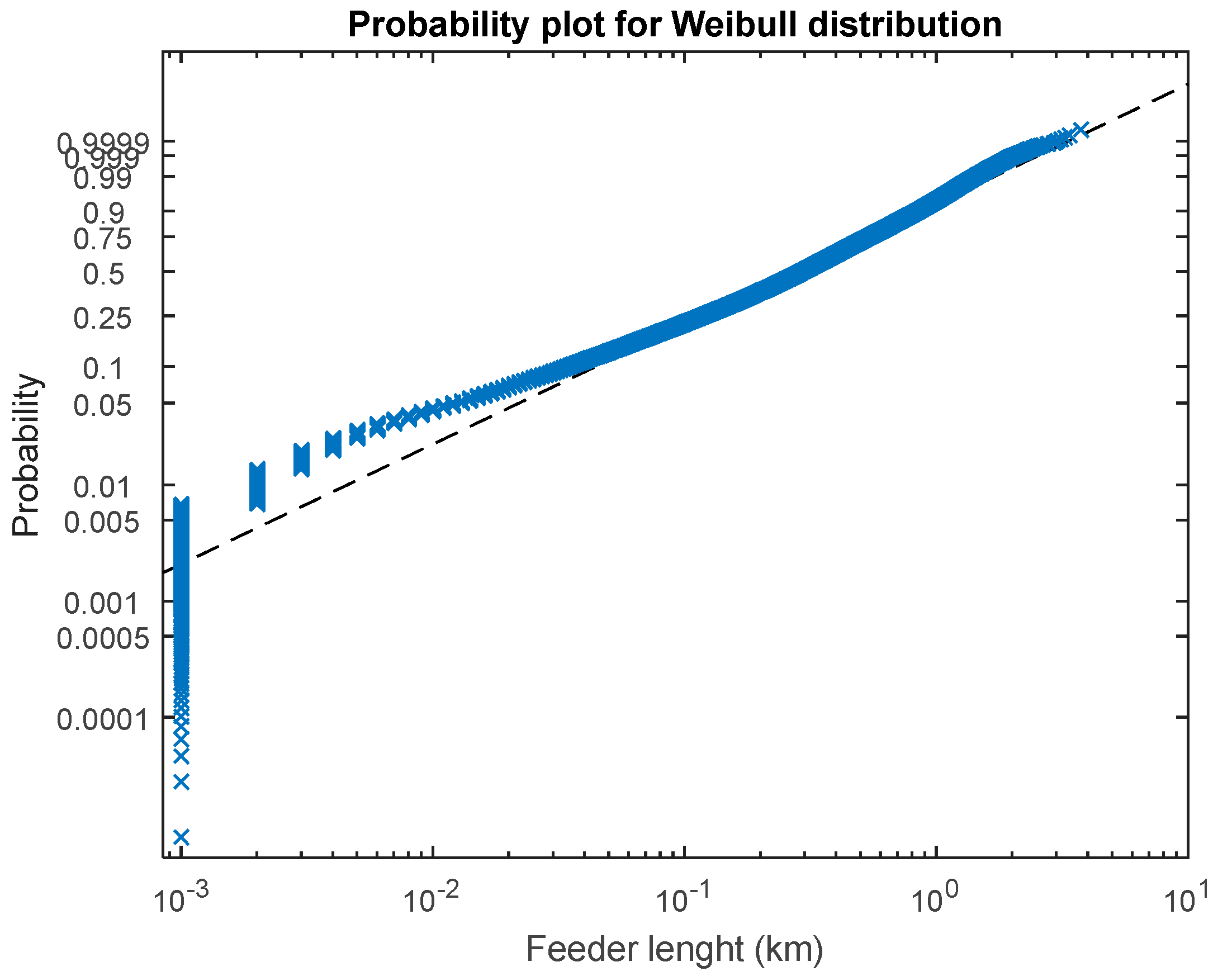
Probability tests can be conducted to any kind of parameters calculated for the feeders. Figure 8 shows exemplarily a probability plot for the feeder length for the network data set of both DSOs. In this particular case, the feeder length (distance from substation to the most distant node) is plotted on a logarithmic scale, whereas the dotted line is indicating a Weibull distribution. In this plot, the raw data were used, where 1% of the feeders have a feeder length of 1 m. This figure shows that rather short feeders (10% of the feeders) do not follow the Weibull distribution. For the majority of feeders (90%), the feeder length could be described by a Weibull-distribution.
With a hypothesis test, the calculated parameters were analyzed if they follow a Weibull distribution with a goodness of fit test (5% significance interval). In Table 2 the parameters that follow a Weibull distribution for each DSO are summarized. Apparently, several parameters are following a Weibull distribution only for one of the two investigated DSOs. Only in the case of DSO A, the average distance to neighbors (ADTN) on feeder level or the short circuit impedance at the equivalent load location follow a Weibull distribution. However, the two DSOs have 3 parameters in common that follow a Weibull distribution. These 3 are related to the end node: the voltage sensitivity on active power (dvdP), the short circuit resistance (RK) and the short circuit impedance (ZK). The last mentioned two parameters are determined by the cable type(s) and the length of the feeder. Consequently, feeder taxonomy based on some particular parameters of one DSO (that may fit very well) may result in supply areas of other DSOs to inaccuracies. Therefore, the selection of parameters to classify feeders shall be well-considered. For studies based on the DER-scenario eof, parameters related to the end node may be one important pillar in DSO-independent feeder taxonomy.
Additionally, for each calculated hosting capability scenario, the voltage and maximal loading were recorded. Therefore, the constraint reason can be identified for each scenario. Consequently, this allows evaluating the share of voltage and current-constrained feeders and the evolution according to the scenario assumptions. Further, the constraint information can be used to mark statistical parameters such as the feeder length (Figure 9). For each bar, the share of voltage-constrained feeders is shown in blue, the share of voltage and current-constrained feeders in purple and the share of current-constrained feeders in red (for the DER scenario “uniform” and umax = 1.03 p.u.). The cumulated distribution function (cdf) plot in black shows that 90% of the feeders are shorter than 977 m and that current-constrained feeders are typically (99th percentile) shorter than 396 m. As one may expect, long feeders (>500 m) are always voltage-constrained. Nevertheless, apparently the feeder length cannot be used as a measure to distinguish between loading/voltage constrained feeders sharply.
At the most distant node in a LV-feeder, a significantly lower hosting capability is expected compared to a node nearby the secondary substation. The highest short circuit impedance at a node in the feeder (ZK) could be a limiting constraint regarding the achievable hosting capability. The cdf of the short circuit impedance (considering the secondary substation) of the weakest node in feeders is depicted in Figure 10. Apparently, feeders which are loading constrained (red), have a rather little impedance and feeders with higher impedance tend to be voltage constrained. However, this parameter is also not suitable to separate accurately between loading and voltage constrained feeders.
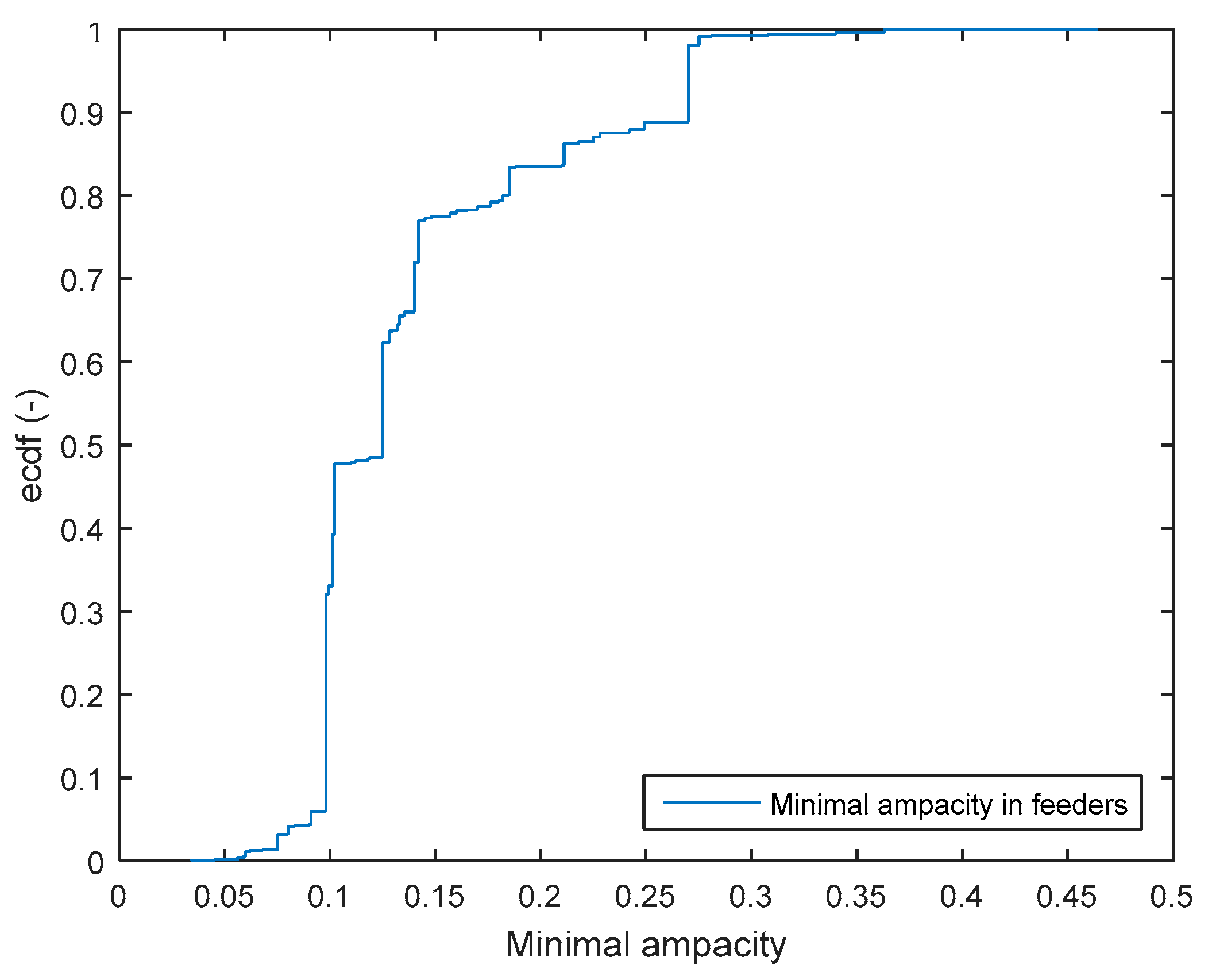
Another constraint limiting the hosting capacity in feeders is the ampacity of lines. In Figure 11, the empirical cumulated distribution function (ecdf) of the lowest ampacity in feeders is depicted. In loading constrained feeders with a uniform DER-distribution, the weakest cable limits the overall hosting capability of the feeder. The distribution shows, that a few cable types are dominating. The lowest ampacity observed in the feeders of the two DSOs are 100 A, 125 A, 140 A and 270 A, equivalent to cable cross sections of NYY-4 × 16 mm2 (NYY: Copper conductors, PVC insulation; 4 wires each with a cable cross-section of 16 mm2), NAYY-4 × 35 mm2 (NAYY: Aluminium conductors, PVC insulation), NAYY-4 × 50 mm2, NAYY-4 × 150 mm2, respectively. Hence, for almost 50% of the feeders, the NYY4 × 16 mm2 (which is mostly used for the service line) may be a bottleneck to increase the hosting capability of feeders. Beside the ampacity, the voltage drop and rise along these cables is significantly higher compared to the main cable conductor of feeders. In [11], it is concluded that a characterization of networks based on the utilized cable types is not feasible and statistics of used cable types in classes of networks is given (rural, sub-urban networks and villages).
3.2. Evaluation of High-Level Indicators to Compare Networks
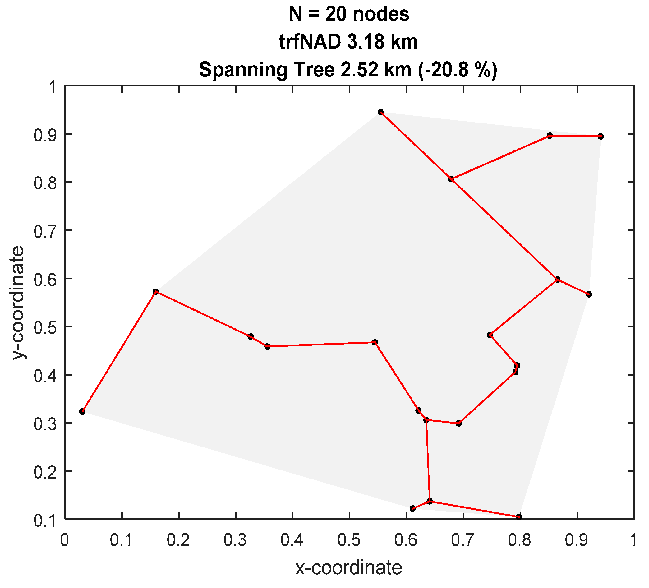
The minimum spanning tree can be used to connect a given number of nodes with a minimal line length. It may be used as an alternative or additionally to the currently used trfNAD indicator [36]. Figure 12 shows an example based on a real network how a spanning Tree could be defined for a given set of connection points (without edge costs). In this example with 20 nodes, the resulting spanning tree length is 2.52 km. The equivalent length according to trfNAD is 3.18 km. For this specific example, the trfNAD indicator turns out to be higher than the spanning Tree Length. In general, this green field approach may not be applicable in certain areas due to geological conditions (railway tracks, historically grown structures, rivers, etc.). A more realistic approach to use the spanning tree (with edge costs) would require defining costs for the entire supply area.
A sensitivity analysis on the impact of the number of nodes in a network on both the trfNAD and the minimum spanning tree length was carried out. The results are depicted in Figure 13. The figure demonstrates that the minimum spanning tree length is higher for networks with less than 10 nodes compared to the trfNAD length. Above 10 nodes, the minimum spanning tree length is smaller and the discrepancy between both measures is increasing with the number of nodes in the network. Consequently, supply areas with a rather high number of nodes would be misleadingly identified as rather inaccurately planned if benchmarked with a minimum spanning tree compared to the trfNAD measure.
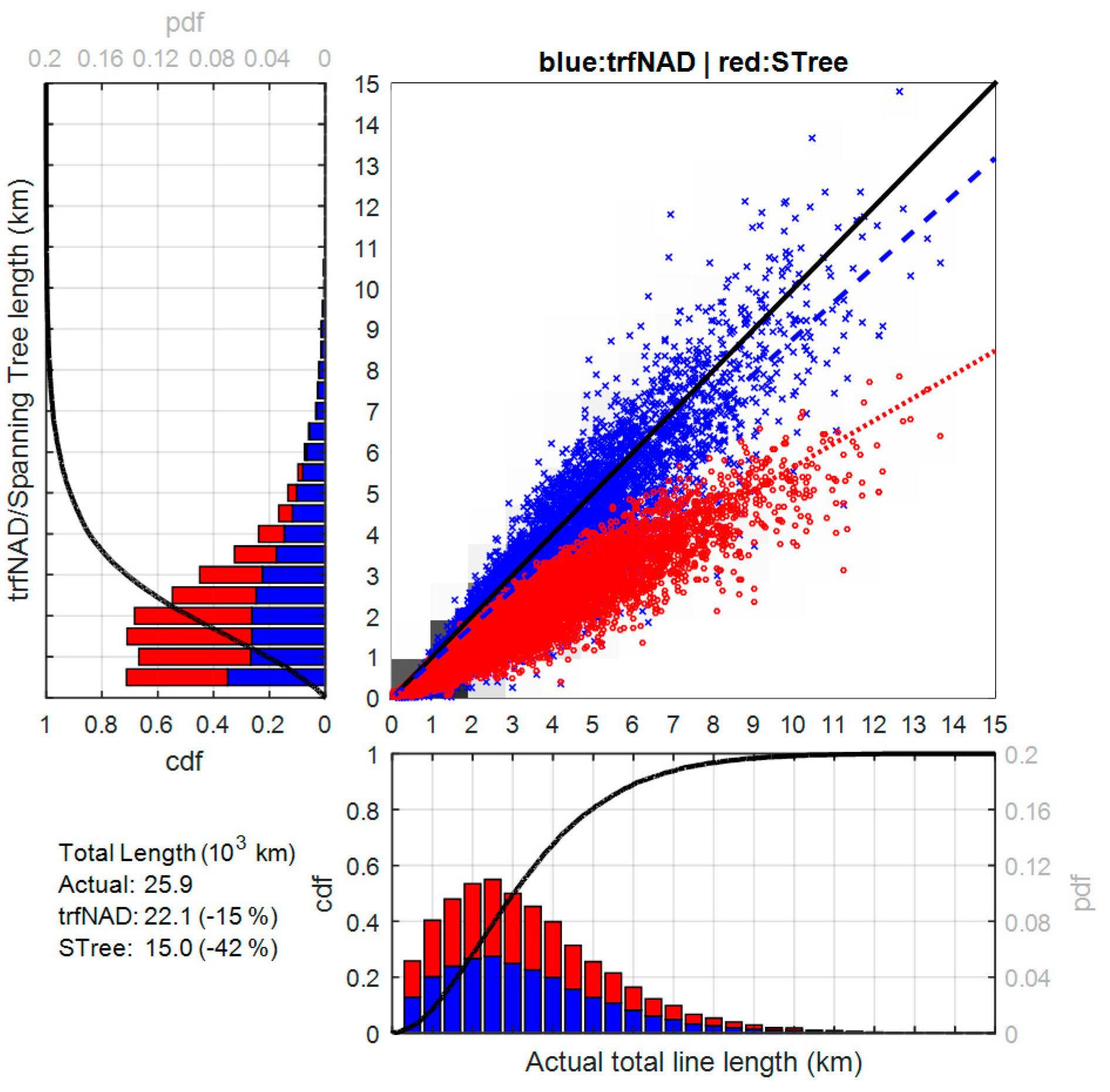
In Figure 14, the evaluation of the spanning tree length compared to the trfNAD parameter is shown for the complete data set of one DSO. The black line indicates the ratio of 1 between the two lengths. The dashed (blue) line shows the linearization of the trfNAD length and the dotted (red) line the spanning tree length. Thereby the mismatch between trfNAD length and the total line length is smaller compared to the spanning tree length. In total, the trfNAD length is 15% lower compared to the actual total cable length and the spanning tree length even 42% lower. Further investigations are needed to investigate the impact of the supply structure on the indicators in order to quantify possible bias between several approaches. One sample network with a rather high mismatch between actual total line length and the spanning tree length was selected to demonstrate justification of reasonable network planning.
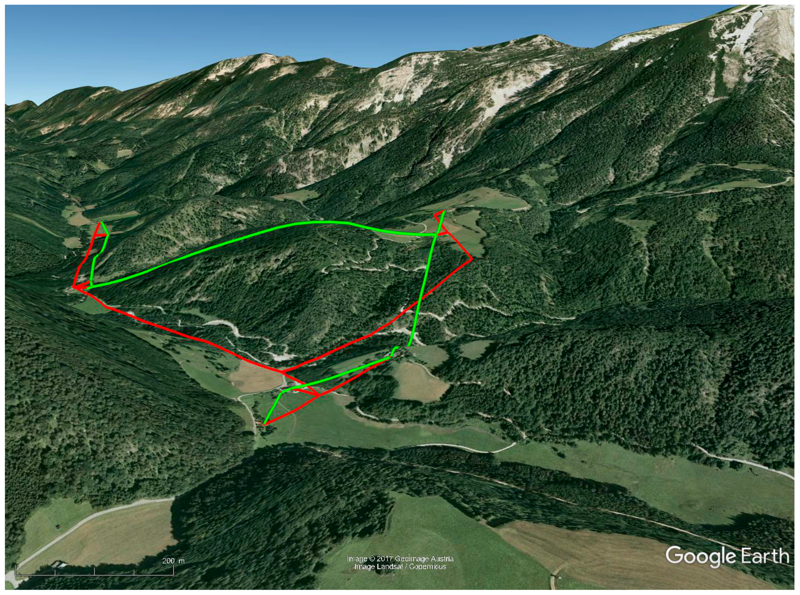
In Figure 15, a network with an actual total line length of 5.2 km is depicted. For this network, the trfNAD length is 4.4 km and the spanning tree length 4.2 km. The theoretical line lengths are about 20% lower than the actual total line lengths. This selected network is a very rural LV network supplying 11 customers, with a mix of over-head lines and cables (70% over-head lines and 30% underground cable). The green lines show the calculated spanning tree to supply the customers with a minimal line length. The red lines mark the actual lines. The geological circumstances, however, show that a major part of the spanning tree passes through a mountainous forest area which should in practice be avoided (for cost and reliability reasons). The actual network (red) is laid in the valley and has therefore a higher total length.
This example shows that comparing distribution networks in an accurate, general, fair and easy way is rather difficult and only meaningful when done for a large population of networks: the used metrics cannot fully capture the network specificities for benchmarking a given network since the local properties are not considered. Moreover, tools from graph theory require the definition of costs of connection of customers to specific substations. The definition of these costs for all customers of a DSO may be a time-consuming task requiring high efforts.
4. Results on the Hosting Capability of Feeders
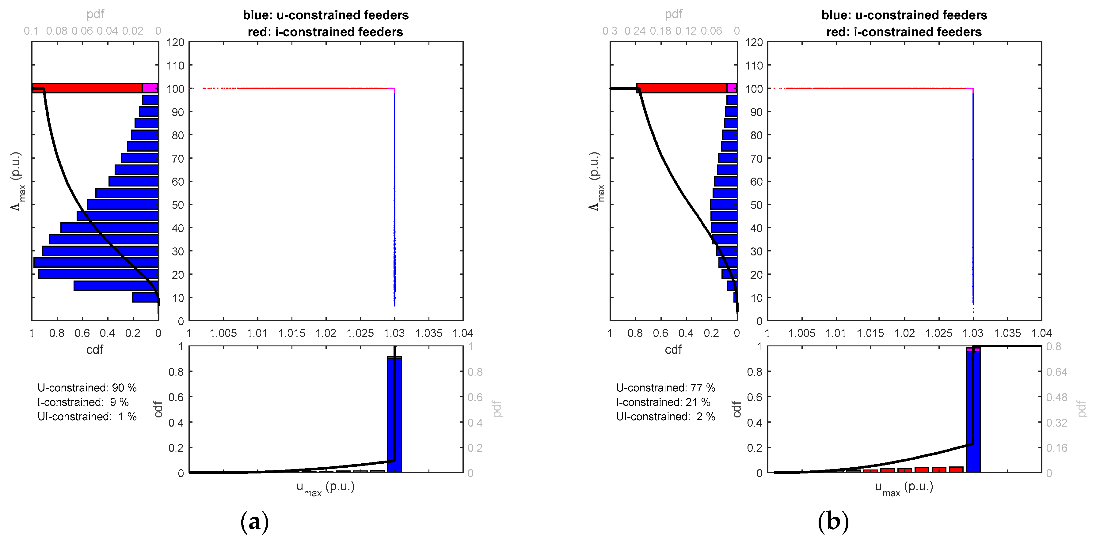
Reactive power control strategies aiming to reduce the voltage rise introduced by DER infeed are causing an additional loading of lines. Before deploying such smart grid solutions, a sufficient reserve in terms of the line rating should be remaining. In Figure 16, the share of voltage (blue) and current (red) constrained feeders on the “U/I plane” is depicted for the two investigated DSOs. Each point on the main part of the figures (upper right) represents a feeder which is colored according to the constraint for an admissible voltage rise of 3%.
In the case of DSO A, Figure 16a shows that about 90% of the feeders are voltage-constrained, confirming that meeting the voltage limits is dominantly limiting the hosting capability for the great majority of feeders Additionally, the plot on the left shows that most of the voltage-constrained feeders (blue) are “far from the corner” (voltage and current constraint) which means that the maximal loading of most of the voltage-constrained feeders is rather far from the 100% loading limit. For 50% of the voltage-constrained feeders, the maximal loading is below 37%, which means that there is a large reserve in respect to overloading lines. Accordingly, there is a priori a large deployment potential of smart grids solutions aiming at controlling the voltage (without observing the loading) without taking the risk or running into overloading network elements.
In the case of DSO B (Figure 16b), the share of loading constrained feeders is significantly higher compared to DSO A. The share of loading constrained feeders is 21% and voltage constrained feeders 77%. Further, fewer feeders have a high loading reserve compared to DSO A. The loading reserve for about 60% of the feeders is less than 50%. Therefore, the share of feeders where the full potential of reactive power control strategies cannot be reached is higher.
One can expect that the DER scenario and the allowed voltage limit have a high impact on the hosting capability of feeders. Furthermore, the constraint reason (voltage or loading) may vary with these assumptions as well. Figure 17 demonstrates that the constraint limiting the hosting capability is rather independent for lower range of voltage limits from the investigated DER scenarios. At umax = 1.01 p.u., almost 100% of the feeders are voltage constrained. For higher voltage limits, the share of voltage constrained feeders is steadily decreasing.
In Figure 17a, less than 40% of the feeders remain voltage constrained at umax = 1.08 p.u. for the DER-scenario uniform. Up to an admissible voltage rise of 4%, the constraint reason is rather independent from the considered DER-scenario. At an admissible voltage limit of 8%, the difference of the constraint reason for the DER scenarios uniform and eof is less than 10%.
With an activated VoltVAr-control (according to [38,39]) for the DER-scenario uniform, a little more feeders remain voltage constrained compared to a PF = 0.9 (Figure 17b). An application of this approach is presented in [35]. With reactive power control the share of loading constrained feeders at umax = 1.08 p.u. reaches 80%, which is significantly higher compared to Figure 17a. In conclusion, the DER-scenario eof is suitable to estimate if a feeder will be either voltage or loading constrained for a given admissible voltage rise under the DER-scenario uniform. In particular, for PF = 1 an estimation up to an admissible voltage rise of 4% is accurate. Considering PF = 0.9 (Figure 17b), for the full range of voltage limits accurate results regarding the constraint reason can be expected.
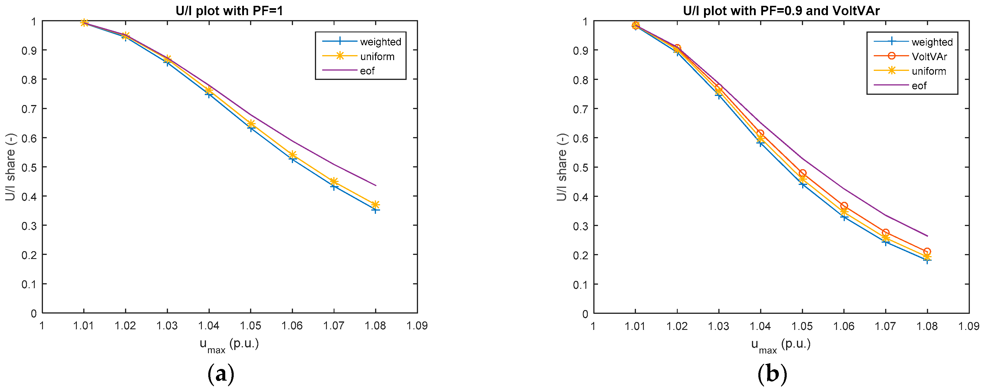
In Figure 18, the HC results for two DER-scenarios (uniform and end of feeder) with and without reactive power control strategies (PF = 1, PF = 0.9 and VoltVAr) are depicted.
In Figure 18a, the distribution of the HC of all feeders for different voltage levels are depicted for the DER-scenario uniform and PF = 1 for both DSOs. Up to 1.07 p.u., a steadily increase of the HC can be observed. At 1.07 p.u. and 1.08 p.u., the 95th percentile remains stable, but the median and the 5th percentile are still increasing by about 10 kW and 5 kW, respectively per voltage step. Concerning the allowed voltage rise, allowing a voltage rise of 1.02 p.u. instead of 1.01 p.u. leads to a significant HC increase. In that case, the median value can be doubled from about 25 kW to more than 50 kW. If the admissible voltage rise can be increased to 4%, more than 50% of the feeders have a HC higher than 100 kW. For higher admissible voltage limits a higher share of feeders become loading constrained. Hence, a voltage increase has no impact on the achievable HC anymore, since a cable in the feeder may be fully loaded. Therefore, the maximal HC is reached.
Next, the HC study results for the DER-scenario uniform and a PF = 0.9 control are depicted in Figure 18b. In this case, the median is always higher compared to the uncontrolled case. The 95th percentile is lower except for 1.01 p.u., 1.02 p.u. and 1.04 p.u., but the 5th percentile is always higher except for the voltage limits of 1.01 p.u. and 1.02 p.u. For the voltage limit 1.05 p.u. and 1.06 p.u., as well as for 1.07 p.u. and 1.08 p.u., similar HC distributions are observed. Compared to the VoltVAr control (DER-scenario uniform), a lower 95th percentile is reached, except for 1.01 p.u. The median HC of both control schemes are comparable for most of the voltage limits. However, regarding the median HC, the VoltVAr control outperforms the PF = 0.9 for higher voltage limits. At an admissible voltage limit of 1.04 p.u., the median is at a comparable level of 120 kW.
Assuming that only one DER is installed in the feeder and is located at the feeder end node, the HC is significantly lower compared to the DER-scenario uniform (Figure 18c). For example, assuming an admissible voltage level of 1.03 p.u., the median value is less than half of the median value for the respective DER-scenario uniform. Further the 95th percentile above voltage limits of 1.04 p.u. remains almost at the same level. However, the 5th percentile and the median are increasing. In addition, in this scenario, a voltage limit of 1.01 p.u. cannot be recommended at all. For the DER-scenario eof, for none of the voltage limits a median value of 100 kW is reached. The calculated HC for this DER-scenario is the minimal HC of the feeder that can be deployed at any node without violating voltage constraints. If the main path from the substation to the end node contains the cable with the lowest ampacity in the feeder, the loading constraint will not be violated as well. Therefore this scenario could be used as benchmark level for the upstream grid to answer the question which amount of DER could be deployed in all supplied feeders without network reinforcements or reactive power control strategies.
In Figure 18d the results for the DER-scenario uniform and VoltVAr-control are shown. Similar to the uncontrolled DER-scenario uniform, a steadily increase of the HC is monitored such that the median HC of the VoltVAr scenario is higher for all voltage limits. However, the HC value of the 99th percentile is not reached (loading constrained feeders). Similar to the DER-scenario uniform, a voltage limit of 1.01 p.u. cannot be recommended. For the voltage limit 1.04 p.u., the median value even reaches 120 kW.
Based on the median HC findings for the DER-scenario uniform in Figure 18, the following suggestions can be given. In most of the cases, extending the voltage band, if possible, by 0.01 p.u., leads to a higher HC value than applying either a PF = 0.9 or a VoltVAr control. At an admissible voltage limit of 1.05 p.u., a PF = 0.9 or a VoltVAr control leads to a similar HC value compared to the HC at an admissible voltage limit of 1.06 p.u. (PF = 1). To increase the median HC at 1.06 p.u. (with PF = 1), increasing the voltage band to 1.07 p.u., or applying a VoltVAr-control (at 1.06 p.u.) can be suggested. At an admissible voltage limit of 1.07 p.u., a VoltVAr-control leads to a higher median HC compared to a voltage band extension to 1.08 p.u. The 5th percentile of the HC with reactive power (PF = 0.9 or VoltVAr—Figure 18b,d) at 1.04 p.u. equals the 5th percentile of the HC at 1.05 p.u. in Figure 18a. Hence, below 1.05 p.u., an extension of the voltage band leads to a higher HC compared to applying a reactive power control. Above 1.05 p.u., the 5th percentile of HC with reactive power control is equal or higher compared to the uncontrolled case with an increased admissible voltage rise. The HC values of the 95th percentiles of the scenarios with a reactive power control are lower compared to the uncontrolled case (PF = 1). Hence, in a first step, it is suggested to increase the admissible voltage rise, if possible, before applying a reactive power control. Due to the increasing share of loading constrained feeders at higher admissible voltage limits, higher HC values can be reached with a VoltVAr-control compared to a PF = 0.9 control.
5. Correlation Results of the Hosting Capability and Particular Parameters of Feeders
In this section, the results of the correlation between feeder parameters and the introduced hosting capability of feeders for a high number of scenarios are presented.
For all parameters summarized in Table 1 the correlation with the hosting capability scenarios was calculated. This approach allows identifying parameters that may be used to estimate the hosting capability without load flow calculations, and are relevant for feeder taxonomy studies.
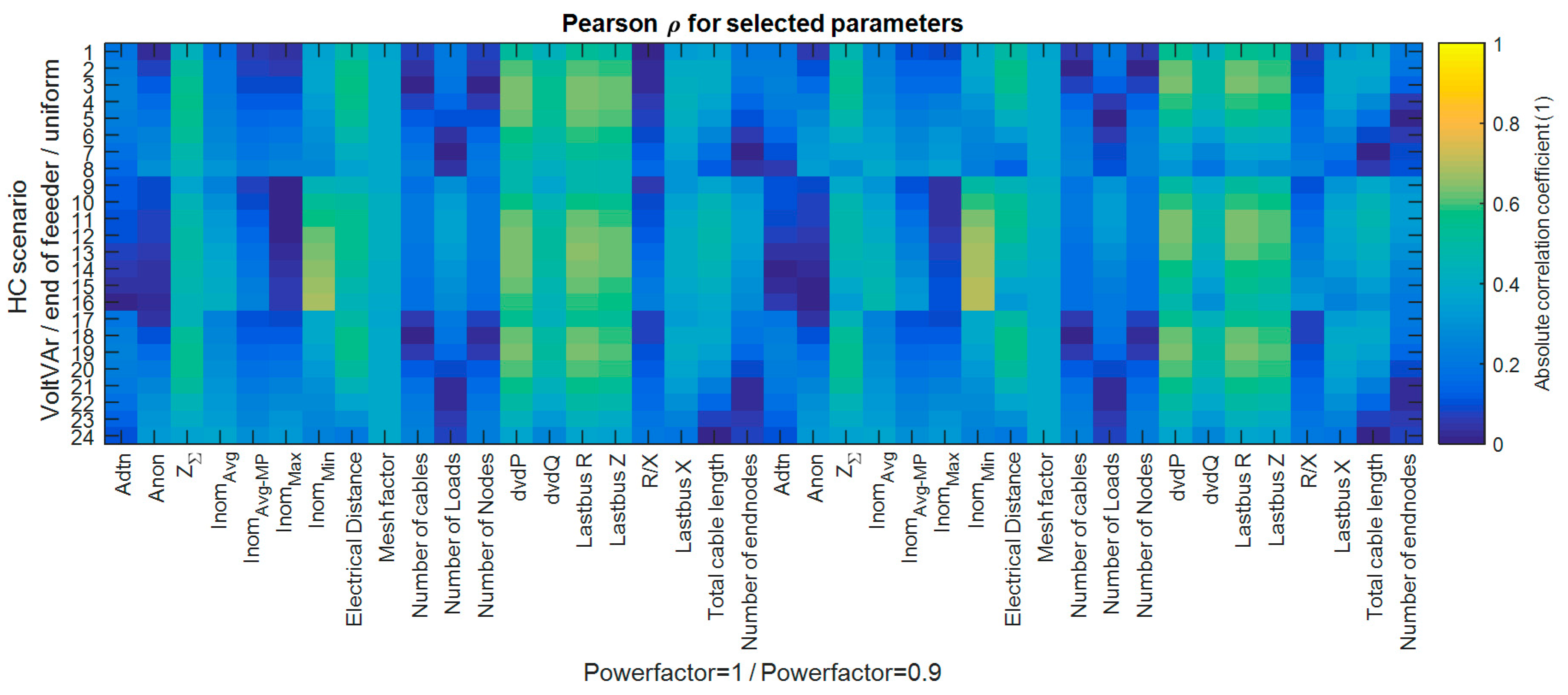
The correlation was calculated for the DER scenarios uniform, eof and additionally for the DER-scenario uniform with activated VoltVAr-control. For each scenario, the hosting capability for a specified allocated voltage band the correlation was performed (Table 3). Further, for the DER scenarios uniform and eof a power factor of 1 and 0.9 was applied (Table 4). Thereby, the combination VoltVAr and HC @ PF = 0.9 is not possible: VoltVAr-results are replicated to the lower left part of the figure.
In Figure 19, the Pearson correlation of all available parameters for two DER-scenarios and the VoltVAr control and voltage limits with the calculated hosting capability is depicted according to the description in the previous tables (Table 3 and Table 4). Thereby, the absolute correlation coefficient between zero and one is depicted. In this case, a value of one equals perfect positive or negative correlation and a value of zero indicates uncorrelated parameters. Each column shows the correlation coefficient for all DER-scenarios and voltage limits with one particular parameter with and without a fixed cosϕ-control. This plot demonstrates that, none of the parameters has a high correlation with the hosting capability. The highest correlation coefficient can be found for the scenario PF = 0.9, an admissible voltage limit of umax = 1.08 p.u. and the DER scenario eof. In this particular case, the correlation coefficient of the related hosting capability and the parameter InomMin (cable in the feeder with the lowest ampacity) is 0.699. At a voltage level of 1.08 p.u., a higher share of the feeders is loading constrained, which explains the relatively high correlation coefficient compared to the other parameters.
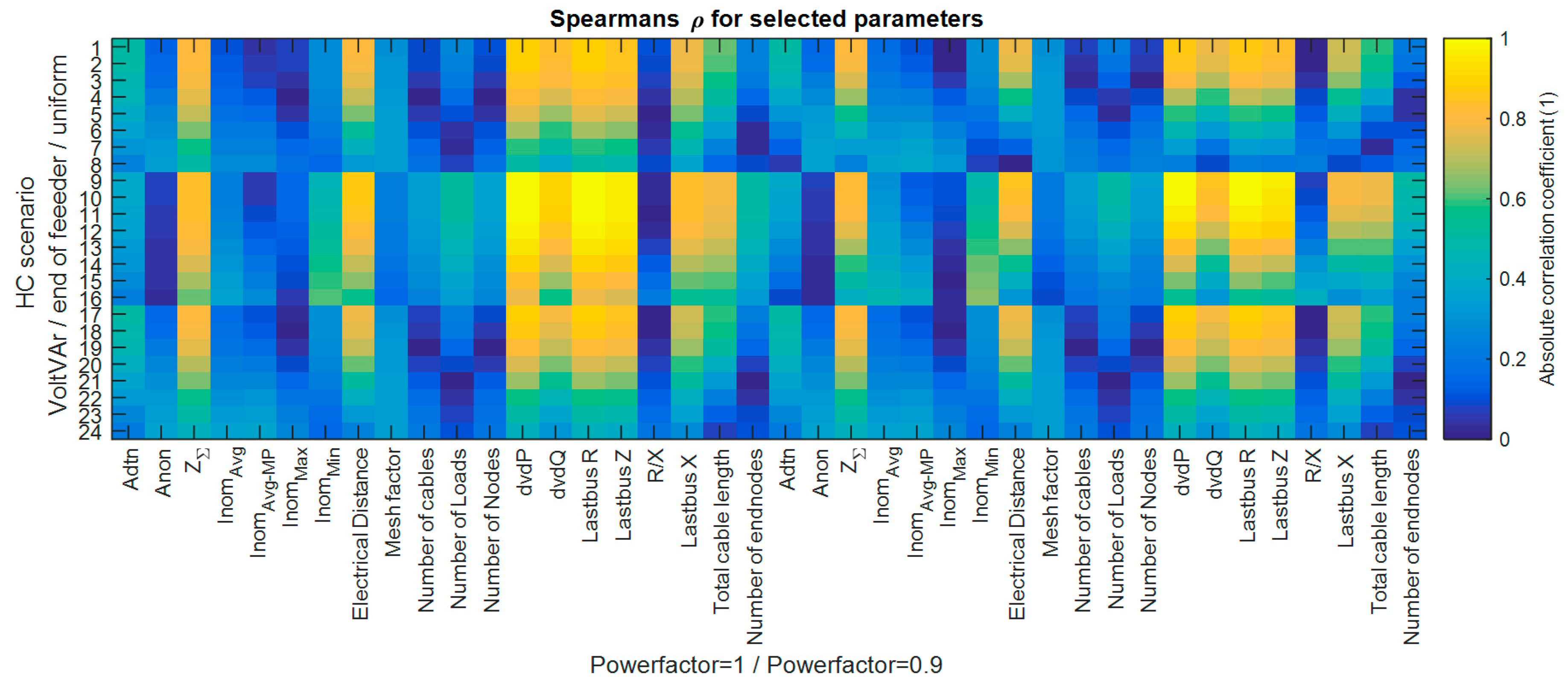
In addition to the Pearson correlation, the Spearman correlation (rank correlation) was also performed for the same input data (Figure 20). For the DER-scenario eof and an admissible voltage limit of 1.01 p.u., perfect correlation is observed for dvdP, ZK and RK. This perfect correlation for this particular scenario is expected, since at an admissible voltage limit of 1.01 p.u. for the DER-scenario eof, almost all feeders are voltage constrained. Then, the hosting capability is determined by the resistance at the end node. Consequently, with higher admissible voltage limits, the share of loading constrained feeders is increasing and the correlation coefficient decreases. Further investigations on feeder taxonomy are ongoing.
Apparently, according to Table 2, the most correlated parameters RK, ZK and dvdP for voltage constrained feeders also follow a Weibull distribution for both DSOs. With each of these parameters, the voltage constrained HC can be estimated for feeders.
6. Conclusions
The presented results show that the developed simulation platform is a powerful tool to analyze the entire LV-grid data of DSOs on feeder level. Due to the modular script design, the calculation can be highly parallelized, keeping the execution time of scripts even for a high number of networks in an acceptable time frame. The platform is capable to calculate the maximal hosting capability per feeder for a high number of scenarios. Moreover, the presented simulation platform was used to identify which constraint limits the hosting capability of the feeders, and whether options other than network reinforcement to increase the hosting capacity are reasonable [35].
To run power flow studies across high-, medium- and low-voltage grids, another option would be to reduce the number of nodes. Therefore, simplified LV-network models are needed to reduce the computational burden. In a future work, simplified LV-feeder models will be defined and validated with the assessed networks. Apparently, out of all investigated parameters, the InomMin (Pearson correlation and higher admissible voltage limits) and the end node resistance (Spearman correlation and lower admissible voltage limits) are the parameters most correlated to the introduced HC, which need to be considered.
The hosting capability results were presented for the DER-scenarios uniform and eof for eight admissible voltage limits ranging from 1% to 8% of the nominal voltage. Moreover, the HC was evaluated with and without reactive power control strategies. In particular, the VoltVAr-control and a fixed cosϕ-control were investigated additionally to the uncontrolled case. Due to the significant HC increase from 1.01 p.u. to 1.02 p.u., an admissible voltage rise limit of 1% cannot be recommended at all. The HC results showed, that increasing the admissible voltage rise for in-feed is only reasonable if a high share of feeders remain voltage constrained. If an admissible voltage rise of 4% is acceptable, for the DER-scenario, uniform more than 50% of the feeders have a HC higher than 100 kW. With a VoltVAr-control, even a median value of 120 kW can be reached. In the worst case scenario, DER-scenario eof, significantly lower median values are achieved. Further, utilizing a reactive power control for loading constrained feeders, leads to a significant HC reduction.
The results on benchmarking showed that different indicators (e.g., minimum spanning tree (without costs) or weighted transformed connection density) could be used to benchmark networks. However, investigations put some bias in evidence when comparing very small and very large networks. These very high-level indicators should therefore be carefully used and further investigations with more DSOs would allow drawing more general conclusions.
The correlation of feeder parameters with the calculated hosting capability values showed that for most of the scenarios no high correlation coefficient could be found. None of the calculated hosting capability values correlate highly with statistical parameters used in literature to classify networks. Further, only a few parameters follow a probability distribution for both investigated DSOs. The described probability plots for selected parameters and feeder statistics however may be used to generate synthetic realistic feeders. Furthermore, the hosting capability results matched with solar resource maps could enable cost-efficient DER deployment plans without investments in grid reinforcement on LV feeder level.
Acknowledgments
This work has been partly sponsored by the project IGREENGrid (IntegratinG Renewables in the EuropEaN Electricity Grid). IGREENGrid project has received funding from the European Union’s Seventh Framework Programme for research, technological development and demonstration under grant agreement No. 308864.
Author Contributions
Benoît Bletterie and Serdar Kadam conceived the idea. Serdar Kadam designed the scenarios and performed the simulations. Benoît Bletterie and Wolfgang Gawlik analyzed the results and provided valuable feedback. Serdar Kadam wrote the paper. Benoît Bletterie and Wolfgang Gawlik critically reviewed the contribution before submission.
Conflicts of Interest
The founding sponsors had no role in the design of the study; in the collection, analyses, or interpretation of data; in the writing of the manuscript, and in the decision to publish the results.
Nomenclature
| ADTN | Average distance to neighbors (m) |
| ANON | Average number of neighbors |
| dvdP | Voltage sensitivity on active power at the end node (%/MW) |
| dvdQ | Voltage sensitivity on reactive power (%/MW) |
| ElDist | Electrical distance to end node (m) |
| eof | End of feeder |
| ε | Equivalent load location, according to [11] |
| GM | Generation momentum |
| MF | Mesh factor |
| NCables | Number of cables |
| NNodes | Number of nodes |
| NLoads | Number of loads |
| NON | Number of neighbors of a node |
| NR | Newton–Rapshon method |
| RK | Short circuit Resistance at end node (Ω) |
| XK | Short circuit reactance at end node (Ω) |
| ZK | Short circuit impedance at end node (Ω) |
| ZΣ | Equivalent sum impedance (Ω), according to [11] |
References
- The International Energy Agency Photovoltaic Power Systems Programme (IEA PVPS). 2014 Snapshot of Global PV Markets. Available online: http://www.iea-pvps.org/fileadmin/dam/public/report/statistics/IEA-PVPS_-__A_Snapshot_of_Global_PV_-_1992-2015_-_Final.pdf (accessed on 19 July 2017).
- Stetz, T.; von Appen, J.; Niedermeyer, F.; Scheibner, G.; Sikora, R.; Braun, M. Twilight of the Grids. Power Energy 2015, 13, 50–61. [Google Scholar] [CrossRef]
- European Photovoltaic Industry Association (EPIA). Global Market Outlook for Photovoltaics 2014–2018. Available online: http://www.cleanenergybusinesscouncil.com/site/resources/files/reports/EPIA_Global_Market_Outlook_for_Photovoltaics_2014-2018_-_Medium_Res.pdf (accessed on 20 July 2017).
- Rekinger, M.; Thies, F. Global Market Outlook for Solar Power 2015–2019. Available online: https://resources.solarbusinesshub.com/solar-industry-reports/item/global-market-outlook-for-solar-power-2015-2019 (accessed on 20 July 2017).
- Greenpeace. Global Wind Energy Outlook 2014. Available online: https://www.gwec.net/wp-content/uploads/2014/10/GWEO2014_WEB.pdf (accessed on 20 July 2017).
- International Energy Agency (IEA). Technology Roadmap-PV. Available online: https://www.iea.org/publications/freepublications/publication/TechnologyRoadmapSolarPhotovoltaicEnergy_2014edition.pdf (accessed on 20 July 2017).
- International Energy Agency (IEA). Technology Roadmap-Wind Energy. Available online: https://www.iea.org/publications/freepublications/publication/Wind_2013_Roadmap.pdf 2013 (accessed on 20 July 2017).
- World Energy Council. World Energy Scenarios-Composing Energy Futures to 2050. Available online: https://www.worldenergy.org/publications/2013/world-energy-scenarios-composing-energy-futures-to-2050/ (accessed on 20 July 2017).
- Nijhuis, M.; Gibescu, M.; Cobben, S. Clustering of low voltage feeders from a network planning perspective. In Proceedings of the CIRED 23rd International Conference on Electricity Distribution, Lyon, France, 15–18 June 2015. [Google Scholar]
- Schlömer, G.; Reese, C.; Hofmann, L. Methode zur Automatisierten Bewertung des Zukünftigen Ausbaubedarfs in der Niederspannungsebene unter Berücksichtigung Verschiedener Technischer Konzepte. Available online: https://www.tugraz.at/fileadmin/user_upload/Events/Eninnov2014/files/kf/KF_Schloemer.pdf (accessed on 20 July 2017).
- Kerber, G. Aufnahmefähigkeit von Niederspannungsverteilnetzen für die Einspeisung aus Photovoltaikkleinanlagen. Ph.D. Thesis, Universität München, München, Germany, March 2011. [Google Scholar]
- Lindner, M.; Aigner, C.; Witzmann, R.; Wirtz, F.; Berber, I.; Gödde, M.; Frings, R. Aktuelle Musternetze zur Untersuchung von Spannungsproblemen in der Niederspannung. Available online: https://www.tugraz.at/fileadmin/user_upload/Events/Eninnov2016/files/kf/Session_E2/KF_Aigner.pdf (accessed on 20 July 2017).
- Kadam, S. Systematical Analysis of Low Voltage-Networks for Smart Grid Studies. Master’s Thesis, Technische Universität, Wien, Austria, June 2012. [Google Scholar]
- Schweitzer, E.; Togawa, K.; Schlösser, T.; Monti, A. A Matlab GUI for the Generation of Distribution Grid Models. In Proceedings of the International ETG Congress 2015, Bonn, Germany, 17–18 November 2015; pp. 79–84. [Google Scholar]
- Jin, S.; Chen, Y.; Diao, R.; Huang, Z.H.; Perkins, W.; Palmer, B. Power grid simulation applications developed using the GridPACKTM high performance computing framework. Electr. Power Syst. Res. 2016, 141, 22–30. [Google Scholar] [CrossRef]
- Santos-Martin, D.; Lemon, S. Simplified Modeling of Low Voltage Distribution Networks for PV Voltage Impact Studies. IEEE Trans. Smart Grid 2016, 7, 1924–1931. [Google Scholar] [CrossRef]
- Bollen, M.H.J.; Sannino, A. Voltage Control with Inverter-Based Distributed Generation. IEEE Trans. Power Deliv. 2005, 20, 519–520. [Google Scholar]
- Dickert, J.; Domagk, M.; Schegner, P. Benchmark low voltage distribution networks based on cluster analysis of actual grid properties. In Proceedings of the 2013 IEEE Grenoble PowerTech (POWERTECH), Grenoble, France, 16–20 June 2013; pp. 1–6. [Google Scholar]
- Ljubic, I.; Weiskircher, R.; Pferschy, U.; Klau, G.W.; Mutzel, P.; Fischetti, M. Solving the Prize-Collecting Steiner Tree Problem to Optimality. Available online: https://www.researchgate.net/profile/Petra_Mutzel/publication/2922227_Solving_the_Prize-Collecting_Steiner_Tree_Problem/links/09e4150eabaf53ec14000000.pdf (accessed on 21 July 2017).
- Schlömer, G.; Hofmann, L. Eine Heuristik zur Umbauplanung von Niederspannungsnetzen ganzer Ortschaften. In Proceedings of the 14 Symposium Energieinnovation, Graz, Austria, 10–12 February 2016. [Google Scholar]
- Tarôco, C.G.; Takahashi, R.H.; Carrano, E.G. Multiobjective planning of power distribution networks with facility location for distributed generation. Electr. Power Syst. Res. 2016, 141, 562–571. [Google Scholar] [CrossRef]
- Bai, H.; Miao, S. Hybrid flow betweenness approach for identification of vulnerable line in power system. IET Gener. Transm. Distrib. 2015, 9, 1324–1331. [Google Scholar] [CrossRef]
- Walker, G.; Nägele, H.; Kniehl, F.; Probst, A.; Brunner, M.; Tenbohlen, S. An application of cluster reference grids for an optimized grid simulation. In Proceedings of the CIRED 23rd International Conference on Electricity Distribution, Lyon, France, 15–18 June 2015. [Google Scholar]
- Li, Y.; Wolfs, P.J. Taxonomic description for western Australian distribution medium-voltage and low-voltage feeders. IET Gener. Transm. Distrib. 2014, 8, 104–113. [Google Scholar] [CrossRef]
- IntegratinG Renewables in the EuropEaN Electricity Grid (IGREENGrid). Available online: http://www.igreengrid-fp7.eu/ (accessed on 20 July 2017).
- PowerFactory DIgSILENT. Available online: http://www.digsilent.de/index.php/products-powerfactory.html (accessed on 19 July 2017).
- Gaunt, C.T.; Namanya, E.; Herman, R. Voltage modelling of LV feeders with dispersed generation: Limits of penetration of randomly connected photovoltaic generation. Electr. Power Syst. Res. 2017, 143, 1–6. [Google Scholar] [CrossRef]
- Stetz, T.; Wolf, H.; Probst, A.; Eilenberger, S.; Saint, D.Y.M.; Kämpf, E.; Braun, M.; Schöllhorn, D. Stochastische Analyse von Smart-Meter Messdaten. In Proceedings of the Intelligent Energy Supply for the Future, Stuttgart, Germany, 11 May–11 June 2012. [Google Scholar]
- Girgis, A.; Brahma, S. Effect of distributed generation on protective device coordination in distribution system. In Proceedings of the LESCOPE 01 2001 Large Engineering Systems Conference on Power Engineering, Halifax, NS, Canada, 11–13 July 2001. [Google Scholar]
- Chaitusaney, S.; Yokoyama, A. Impact of protection coordination on sizes of several distributed generation sources. In Proceedings of the 2005 International Power Engineering Conference, Singapore, 29 November–2 December 2005. [Google Scholar]
- Papaspiliotopoulos, V.A.; Kleftakis, V.A.; Kotsampopoulos, P.C.; Korres, G.N.; Hatziargyriou, N.D. Hardware-in-the-loop simulation for protection blinding and sympathetic tripping in distribution grids with high penetration of distributed generation. In Proceedings of the MedPower 2014, Athens, Greece, 2–5 November 2014. [Google Scholar]
- Schwaegerl, C.; Bollen, M.H.J.; Karoui, K.; Yagmur, A. Voltage control in distribution systems as a limitation of the hosting capacity for distributed energy resources. In Proceedings of the 18th International Conference and Exhibition on Electricity Distribution (CIRED 2005), Turin, Italy, 6–9 June 2005. [Google Scholar]
- Walker, G.; Schweinfort, W.; Krauss, A.K.; Eilenberger, S.; Tenbohlen, S.; Energiewende, D. Entwicklung eines standardisierten Ansatzes zur Klassifizierung von Verteilnetzen. In Proceedings of the VDE-Kongress, Frankfurt, Germany, 20–21 Octorber 2014. [Google Scholar]
- E-CONTROL. Regulierungssystematik für die Dritte Regulierungsp Eriode der Stromverteilernetzbetreiber 1 Jänner 2014–31 Dezember 2018. Available online: https://www.e-control.at/documents/20903/-/-/225b49e0-6534-40e4-afa1-97d83f8edbdeB (accessed on 21 July 2017).
- Bletterie, B.; Kadam, S.; Priewasser, A.A.R. Statistical Analysis of the Deployment Potential of Smart Grids Solutions to Enhance the Hosting Capacity of LV Networks. Available online: https://www.tugraz.at/fileadmin/user_upload/Events/Eninnov2016/files/lf/Session_E4/LF_Bletterie.pdf (accessed on 21 July 2017).
- Montoya, D.P.; Ramirez, J.M. A minimal spanning tree algorithm for distribution networks configuration. In Proceedings of the 2012 IEEE Power and Energy Society General Meeting, San Diego, CA, USA, 22–26 July 2012. [Google Scholar]
- Kadam, S.; Bletterie, B. A Comprehensive Study on the Actual Potential of Grid Support Functions to Enhance the Hosting Capacity of Distribution Networks with a High PV Penetration. In Proceedings of the 6th Solar Integration Workshop, Vienna, Austria, 14–15 Octorber 2016. [Google Scholar]
- Kadam, S.; Bletterie, B.; Lauss, G.; Heidl, M.; Winter, C.; Hanek, D.; Abart, A. Evaluation of voltage control algorithms in smart grids: Results of the project: MorePV2grid. In Proceedings of the 29th European Photovoltaic Solar Energy Conference and Exhibition, Amsterdam, The Netherlands, 22–26 September 2014. [Google Scholar]
- Heidl, M. MorePV2grid-More Functionalities for Increased Integration of PV into Grid. Available online: https://www.klimafonds.gv.at/assets/Uploads/Blue-Globe-Reports/Erneuerbare-Energien/2012-2013/BGR0062013EEneueEnergien2020.pdf (accessed on 21 July 2017).
Figure 1.
Automated network data import.
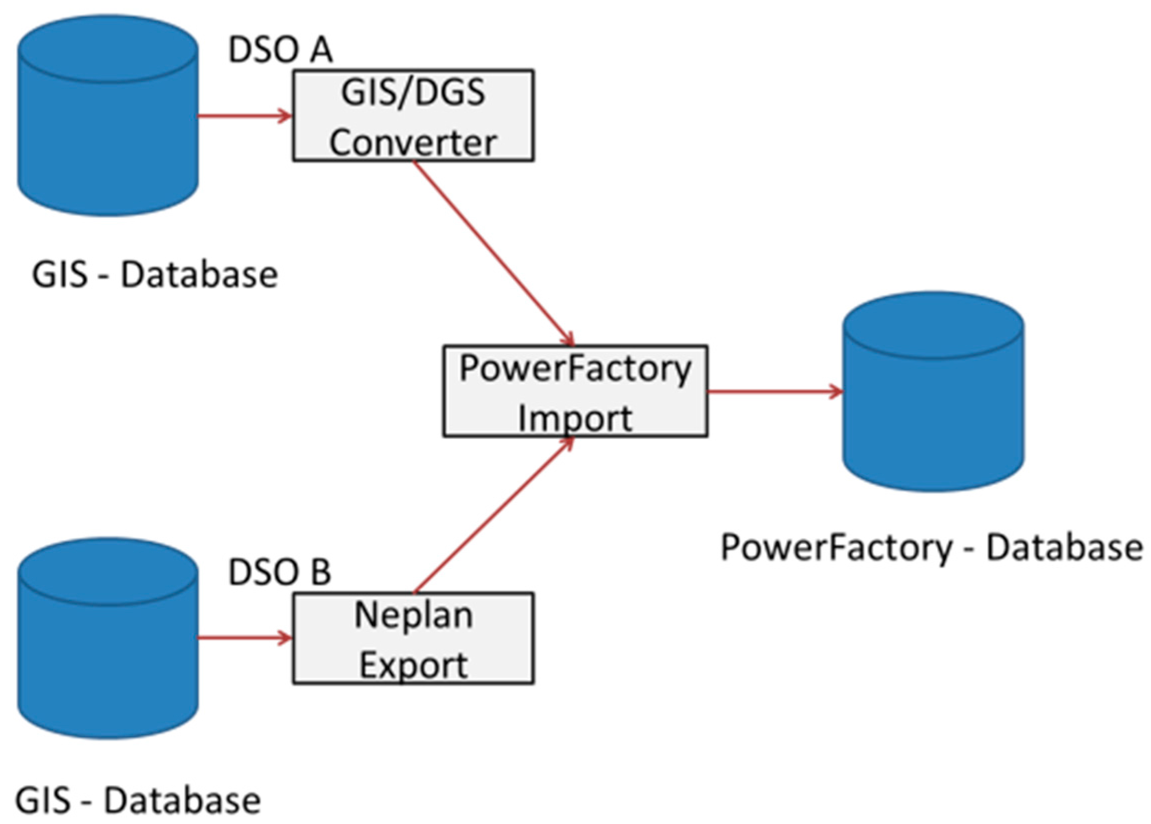
Figure 2.
Considered scenarios.

Figure 3.
Considered Q(U)-control.

Figure 4.
Constraints limiting the hosting capacity.

Figure 5.
Adapted Newton-Raphson (NR)-optimization.
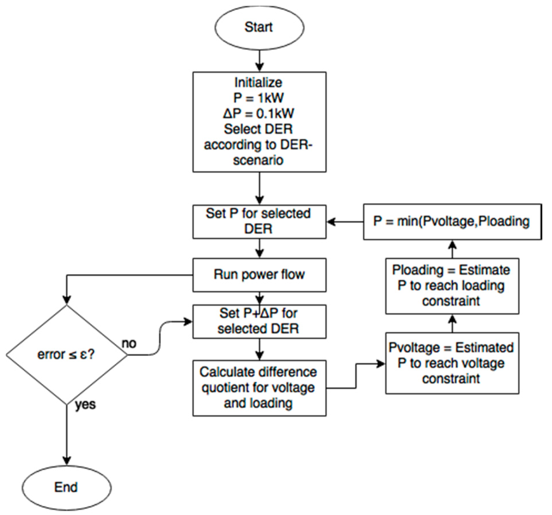
Figure 6.
Algorithm to calculate the feeder hosting capability (HC) for different.

Figure 7.
Simulation output.
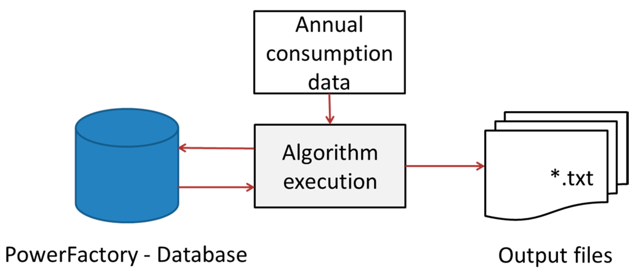
Figure 8.
Weibull probability test of feeder length.

Figure 9.
Cumulated distribution function of the electrical feeder length (red loading constrained, blue voltage constrained and purple loading and voltage constrained).
Figure 9.
Cumulated distribution function of the electrical feeder length (red loading constrained, blue voltage constrained and purple loading and voltage constrained).
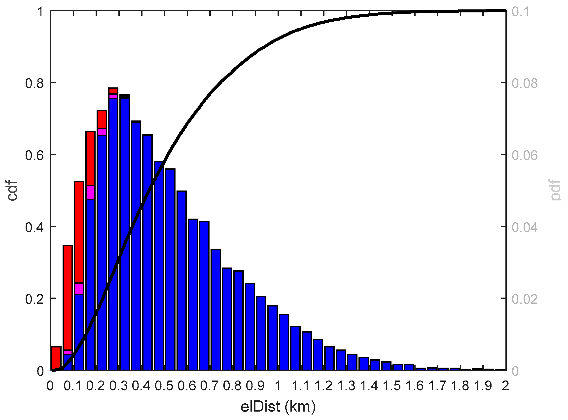
Figure 10.
cdf of the short circuit impedance of the weakest node of feeders (red loading constrained, blue voltage constrained and purple loading and voltage constrained).
Figure 10.
cdf of the short circuit impedance of the weakest node of feeders (red loading constrained, blue voltage constrained and purple loading and voltage constrained).
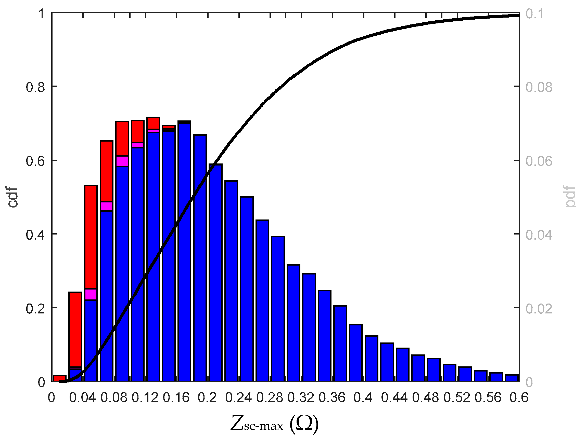
Figure 11.
Ecdf of the minimal ampacity of feeders.

Figure 12.
Example Minimum spanning tree.

Figure 13.
Normalized Line Length Comparison.
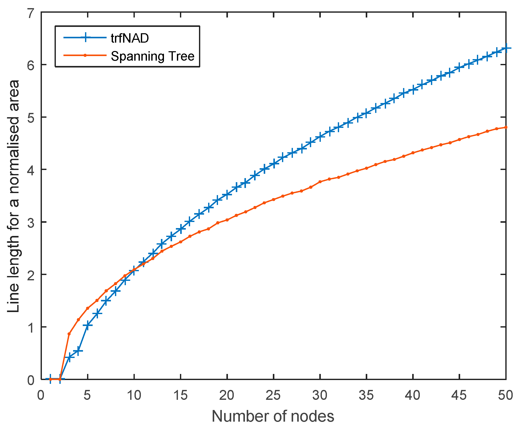
Figure 14.
Comparison: trfNAd (blue) and spanning tree length (red).

Figure 15.
Example demonstrating difficulties of benchmarking.

Figure 16.
Voltage/current constraint assessment of feeders (red: loading constrained, blue: voltage constrained and purple: loading and voltage constrained) for: (a) DSO A; and (b) DSO B (colored according to the DER-scenario uniform and umax = 1.03 p.u. presented in [37]).
Figure 16.
Voltage/current constraint assessment of feeders (red: loading constrained, blue: voltage constrained and purple: loading and voltage constrained) for: (a) DSO A; and (b) DSO B (colored according to the DER-scenario uniform and umax = 1.03 p.u. presented in [37]).

Figure 17.
Share of voltage- and current-constrained feeders. umax = [1.01–1.08] p.u. – Imax = 100% DER scenario: uniform, end of feeder, weighted-and a power factor of 1. (a) PF = 1; and (b) PF = 0.9 and VoltVAr. The DER-scenario uniform was applied for the case VoltVAr.
Figure 17.
Share of voltage- and current-constrained feeders. umax = [1.01–1.08] p.u. – Imax = 100% DER scenario: uniform, end of feeder, weighted-and a power factor of 1. (a) PF = 1; and (b) PF = 0.9 and VoltVAr. The DER-scenario uniform was applied for the case VoltVAr.

Figure 18.
Hosting Capability results of selected scenarios: (a) DER-scenario uniform, PF = 1; (b) DER-scenario uniform, PF = 0.9; (c) DER-scenario eof, PF = 1; and (d) DER-scenario uniform, VoltVAr [37].
Figure 18.
Hosting Capability results of selected scenarios: (a) DER-scenario uniform, PF = 1; (b) DER-scenario uniform, PF = 0.9; (c) DER-scenario eof, PF = 1; and (d) DER-scenario uniform, VoltVAr [37].
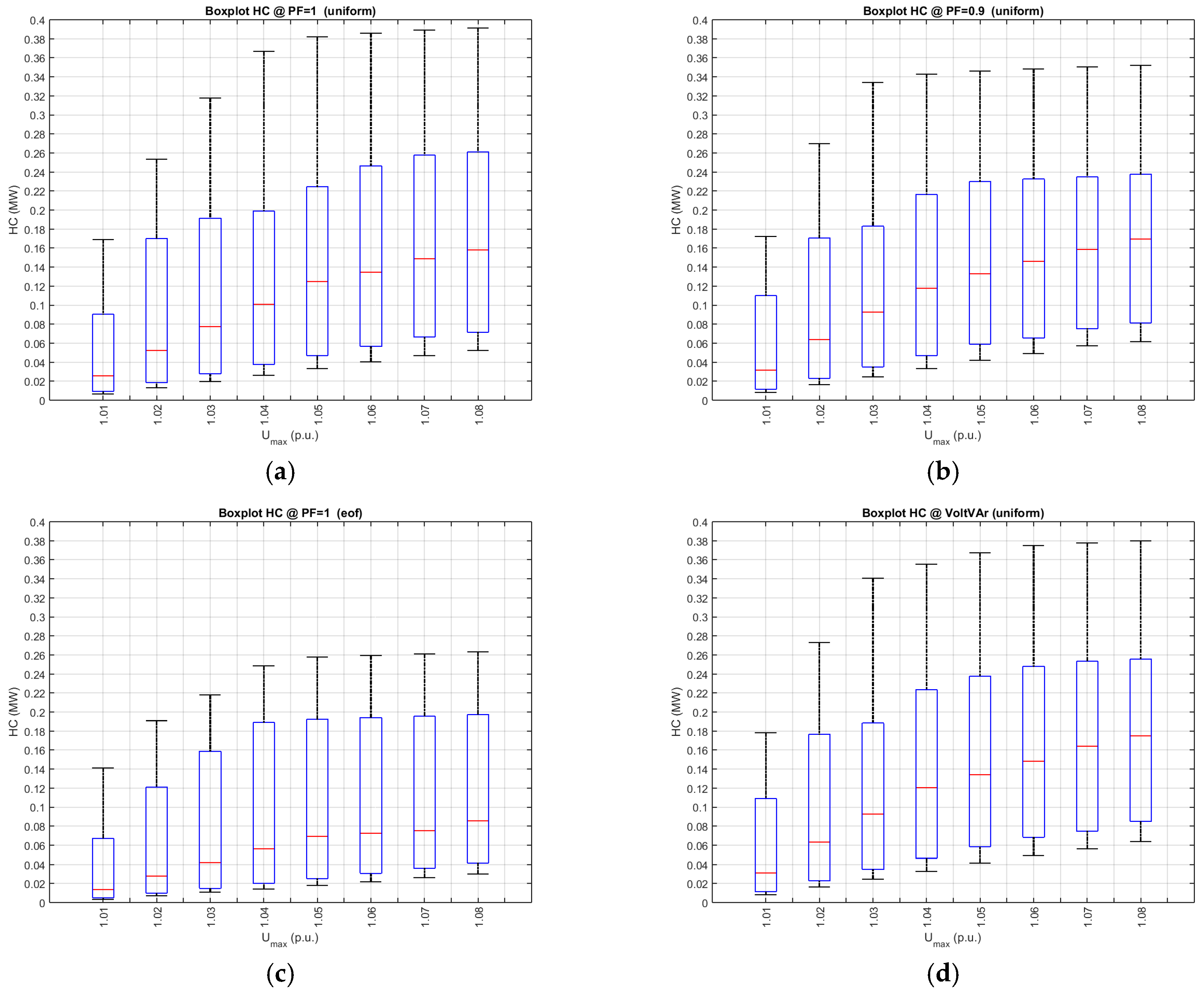
Figure 19.
Pearson correlation (HC @ PF = 1 columns 1–8, HC @ PF = 0.9 columns 9–16, HC @ VoltVar columns 17–24).
Figure 19.
Pearson correlation (HC @ PF = 1 columns 1–8, HC @ PF = 0.9 columns 9–16, HC @ VoltVar columns 17–24).

Figure 20.
Spearman correlation (HC @ PF = 1 columns 1–8, HC @ PF = 0.9 columns 9–16, HC @ VoltVar columns 17–24).
Figure 20.
Spearman correlation (HC @ PF = 1 columns 1–8, HC @ PF = 0.9 columns 9–16, HC @ VoltVar columns 17–24).


Table 1.
Parameters under test and set of parameters for validation purposes.
| Parameters under Test to Classify Feeders | Parameters Available to Validate a Feeder Classification (Including Sensitivity Study on the DER Distribution and the Admissible Voltage Rise) |
|---|---|
| NLoads NNodes NCables ANON (Equation (2)) ADTN (Equation (3)) Cable rating (min, mean, max) Total cable length MF (Equation (4)) ZK, RK, XK ElDist ZΣ (Equation (5)) dvdP (%/MW) dvdQ (%/MVAr) | HC GM (Equations (6) and (7)) ε |
Table 2.
Parameters of each DSO following a Weibull distribution marked with X (significance interval: 5%).
Table 2.
Parameters of each DSO following a Weibull distribution marked with X (significance interval: 5%).
| DSO | ADTN-Feeder | ADTN-Grid | ZΣ (Ω) | ZK at Equivalent Load Location | dvdP (%/MW) |
| DSO A | X | - | X | X | X |
| DSO B | - | X | - | - | X |
| DSO | End Node RK (Ω) | End Node ZK (Ω) | End Node R/X | Losses (MW) | HC (MW) at umax = 1.03 p.u. |
| DSO A | X | X | - | - | - |
| DSO B | X | X | X | X | X |
Table 3.
Investigated scenarios.
| Rows | DER-Scenario | Admissible Voltage Rise |
|---|---|---|
| 1 to 8 | uniform | umax = 1.01 p.u. to 1.08 p.u. |
| 9 to 16 | eof | |
| 17 to 24 | VoltVAr |
Table 4.
Column Groups.
| Columns 1 to 18 | Columns 19 to 36 |
|---|---|
| HC @ PF = 1 | HC @ PF = 0.9 |
© 2017 by the authors. Licensee MDPI, Basel, Switzerland. This article is an open access article distributed under the terms and conditions of the Creative Commons Attribution (CC BY) license (http://creativecommons.org/licenses/by/4.0/).
Share and Cite
MDPI and ACS Style
Kadam, S.; Bletterie, B.; Gawlik, W. A Large Scale Grid Data Analysis Platform for DSOs. Energies 2017, 10, 1099. https://doi.org/10.3390/en10081099
AMA Style
Kadam S, Bletterie B, Gawlik W. A Large Scale Grid Data Analysis Platform for DSOs. Energies. 2017; 10(8):1099. https://doi.org/10.3390/en10081099
Chicago/Turabian StyleKadam, Serdar, Benoît Bletterie, and Wolfgang Gawlik. 2017. "A Large Scale Grid Data Analysis Platform for DSOs" Energies 10, no. 8: 1099. https://doi.org/10.3390/en10081099
Note that from the first issue of 2016, this journal uses article numbers instead of page numbers. See further details here.