A PMU-Based Method for Smart Transmission Grid Voltage Security Visualization and Monitoring

Department of Electrical Engineering, Feng Chia University (FCU), No. 100, Wenhwa Road, Seatwen, Taichung 40724, Taiwan
*
Author to whom correspondence should be addressed.
Energies 2017, 10(8), 1103; https://doi.org/10.3390/en10081103
Submission received: 26 June 2017
/
Revised: 18 July 2017
/
Accepted: 25 July 2017
/
Published: 27 July 2017
(This article belongs to the Collection Smart Grid)
Abstract
:With the rapid growth of usage of phasor measurement units (PMUs) for modern power grids, the application of synchronized phasors (synchrophasors) to real-time voltage security monitoring has become an active research area. This paper presents a novel approach for fast determination of loading margin using PMU data from a wide-area monitoring system (WAMS) to construct the voltage stability boundary (VSB) of a transmission grid. Specifically, a new approach for online loading margin estimation that considers system load trends is proposed based on the Thevenin equivalent (TE) technique and the Mobius transformation (MT) technique. A VSB is then computed by means of real-time PMU measurements and is presented in a complex load power space. VSB can be utilized as a visualization tool that is able to provide real-time visualization of the current voltage stability situation. The proposed method is fast and adequate for online voltage security assessment. Furthermore, it enables us to significantly increase a system operator’s situational awareness for operational decision making. Simulation studies were carried out using different sized power grid models under various operating conditions. The simulation results are shown to validate the capability of the proposed method.
1. Introduction
Recently, voltage stability has become a challenging issue in power industries since several major blackouts worldwide have been mainly attributed to voltage collapse [1,2,3]. Based on this concern, much attention has been devoted to understanding the voltage collapse phenomenon. Voltage collapse is described as the phenomenon in which the events in sequential operations are accompanied by voltage instability. This may lead to blackouts or abnormally low voltage distribution in a vital part of the power grid [4,5]. Therefore, it is essential that system operators easily identify system voltage instability to prevent possible voltage collapse.
In view of this, a variety of methods have been proposed for static voltage security analysis, such as sensitivity methods [6,7], continuation power flow (CPF) methods [8,9], and impedance match methods [10,11,12,13,14,15]. Indeed, the Power-Voltage (P-V) curve is widely utilized for voltage stability analysis. Generally, such a curve is produced by calculating power flow solutions for successively increasing load levels. To cope with the divergence issue of power flow calculation near the point of voltage collapse, the CPF methods are presented [8,9]. Since the CPF methods belong to model-based tools, a large amount of computation time for a bulk power grid model is required. In addition, an accurate system model is needed for this kind of model-based approach. According to the description above, CPF methods are not suitable for online voltage stability analysis in its current setting. In contrast, impedance match methods are measurement-based tools for online voltage stability monitoring [10,11,12,13,14,15]. Such methods are based on Thevenin equivalent (TE) impedance matching criterion using measured voltage and current phasors. As voltage instability take places at a load bus, the load impedance is equal to the TE impedance in magnitude. As a consequence, the difference between the load impedance and TE impedance can be utilized as an index for voltage stability monitoring. Even though the impedance margin can be employed to determine whether the present operating condition is voltage secure, loading margin information, which is more useful for system planners and operators, becomes obscure. Hence, an alternative approach is required.
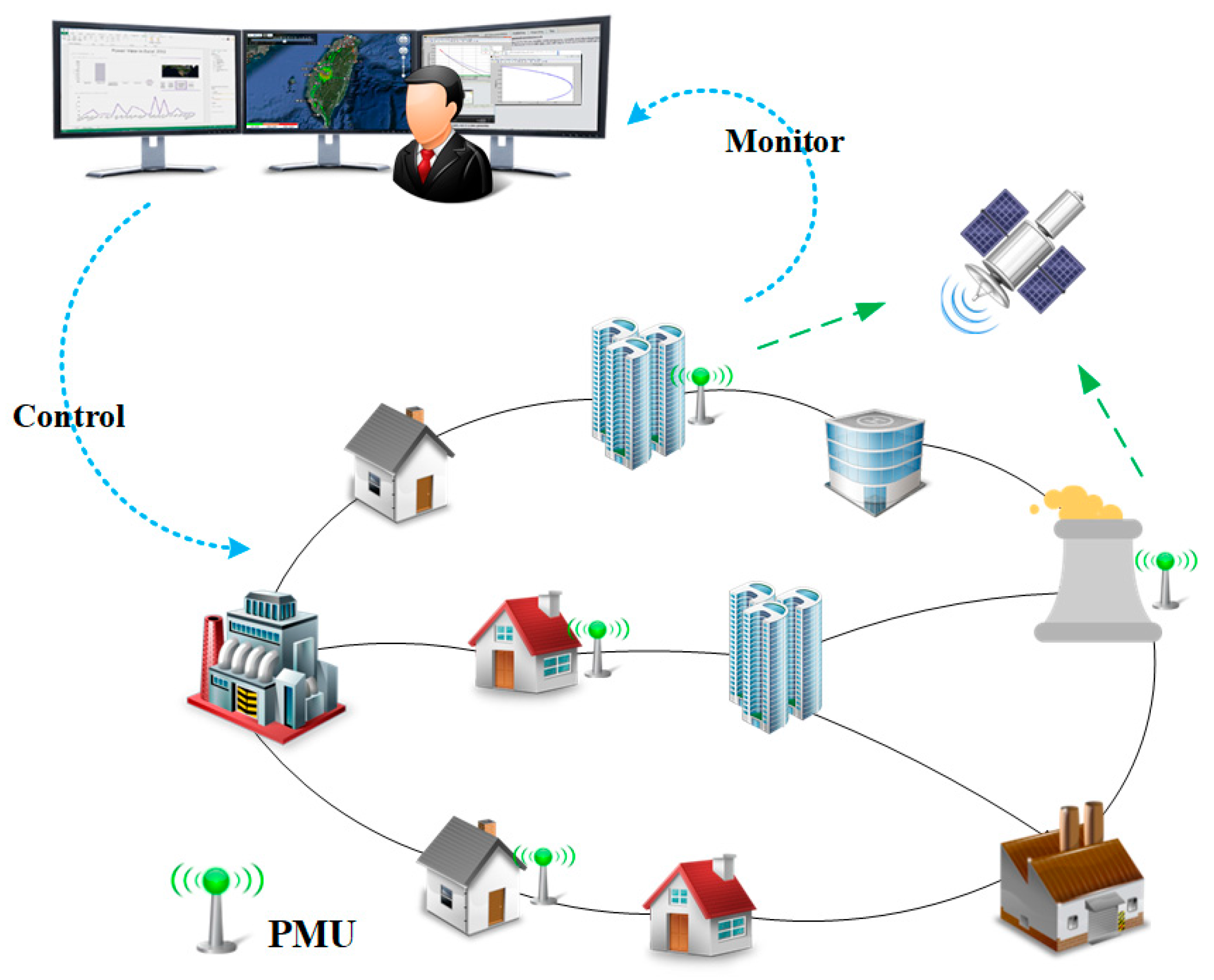
The wide area monitoring system (WAMS) is expected to be a core technology in future smart grids [16,17]. With the gradual installation of phasor measurement units (PMUs) in many power grids, the PMU-based WAMS is becoming indispensable to sustaining reliability and security for modern power grids. PMUs, which are an advanced and fully developed technology, have been produced by many international manufacturers. Furthermore, most of the PMUs available on the market follow the IEEE standard C37.118, which defines frequency, rate of change of frequency, and synchronized phasors (synchrophasors) under all power system operating conditions. A more detailed description about this standard can be found in [18]. Figure 1 illustrates a typical structure of a PMU-based WAMS in a smart grid. Indeed, the wide-area measurements from PMUs, which is coherent and time-synchronized, can help increase real-time situational awareness for system operators to carry out time-critical tasks under critical conditions. This indicates that the PMU-based WAMS serves great opportunity to reconfigure the power system before reaching the voltage collapse point and avoid power system blackouts.
This research is mainly devoted to smart transmission grid voltage security visualization and monitoring. The contribution of this paper is the development of a novel method which aims to advance wide-area situational awareness enhanced with voltage stability monitoring. To this end, a new algorithm based on the Thevenin equivalent (TE) technique and the Mobius transformation (MT) technique for online system loading margin estimation is proposed. The approximation of a voltage stability boundary (VSB) can then be obtained by a quadratic curve using PMU data. The computed VSB can provide real-time visualization of the current voltage stability situation. This enables a significant increase in the system operator’s situational awareness for operational decision making. Furthermore, the proposed method is simple and fast, which makes it adequate for online applications.
The rest of this work is as follows: The impedance match method to static voltage stability analysis is briefly reviewed in Section 2. Section 3 describes the proposed method, and some computational details are discussed. The proposed method is tested on several Electrical and Electronics Engineers (IEEE) power grid models under various operating conditions in Section 4. Section 5 gives some concluding remarks.
2. Review of the Impedance Match Method to Static Voltage Stability Analysis
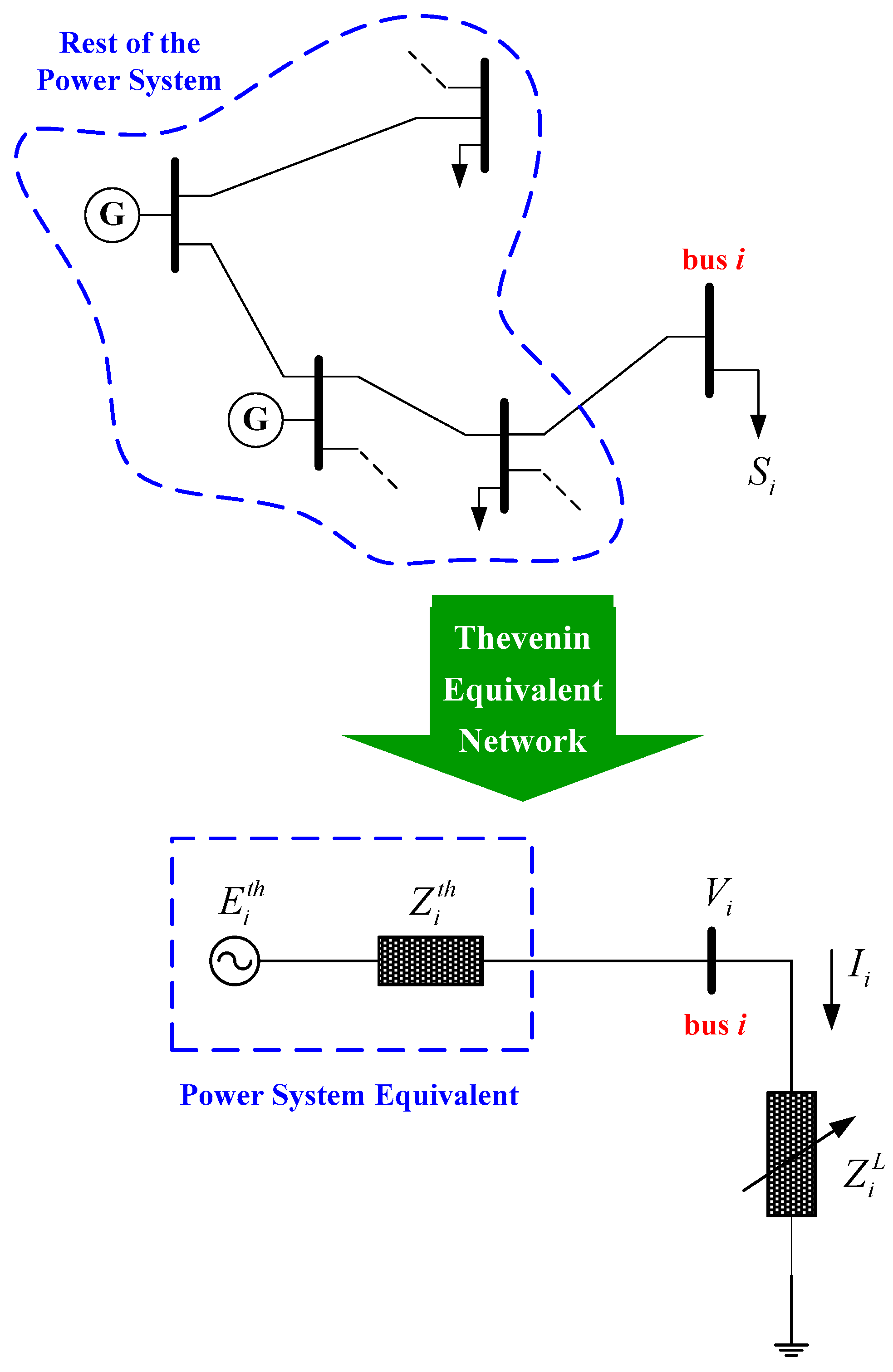
Impedance match methods are measurement-based tools for static voltage stability analysis [10,11,12,13,14,15]. Such methods use the concept of tracking the Thevenin equivalent (TE) parameters for a power system at a node using local voltage and current phasor measurements.
A complex power grid seen at a load bus i can be simplified to a TE network, shown in Figure 2, in which is the TE voltage, is the TE impedance, and is the load impedance at load bus i. Note that , , and are all in phasor representation,
In this research, the phasors are in per units, the magnitudes are in per units, and the angles are in degrees.
A key idea of the impedance match method is summarized as follows: when voltage collapse occurs, . Consequently, the ratio of can be utilized as an index for voltage stability monitoring, as shown in Figure 3. If the ratio is smaller than 1, the system will be stable. On the other hand, if the ratio is higher than 1, the system is unstable.
Due to the elegance and simplicity of this impedance-matching concept, the measurement-based real-time voltage stability analysis becomes possible [10,11,12,13,14,15]. The impedance-based index methods can be adopted to identify if a given operating condition is within a secure voltage margin or not. The information of the loading margin, however, becomes obscure. To address these difficulties, a new method, which is able to provide loading margin, is proposed in this research.
3. Proposed Method
This section presents a new method to transmission grid voltage stability visualization and monitoring utilizing PMU measurements. The main steps in the proposed method are shown in Figure 4 and are described in the following subsections.
3.1. Determination of Load Increase Direction
Loading margin estimations depend on load levels and load increase directions (LIDs). To illustrate this, Figure 5 shows the voltage collapse (critical point) surface in a load power parameter space with active and reactive load powers as coordinates. In Figure 5, let be the initial point, and and be two distinct LIDs, respectively. If increases along the direction of , the maximum loading point would be . Instead, if follows , the critical point would be . Clearly, distinct LIDs result in distinct voltage collapse points. Thus, it is essential to estimate the voltage collapse point with consideration of the LID.
The complex load power change is typically expressed as,
where
In the above equations, and denote voltage and current measurements at load bus i, and t denotes the tth sampling point. In this research, the LID is accomplished by using two sets of consecutive PMU measurements.
3.2. Estimation of Thevenin Equivalent Network Parameters
In Figure 2, application of Kirchoff’s voltage law to TE network yields,
where and denote the load voltage and current phasors. Suppose that the data points of and are available from the installed PMU. The unknown variables in Equation (5) are and . Since the Thevenin equivalent parameters is approximately constant under various loading conditions [10,11,12,13,14,15], and can be determined by using two data pairs and as,
From the preceding equations, TE network for a power system at a bus can be acquired. Moreover, the load impedance can be obtained by,
where denotes the conjugate of the complex load power .
According to Equations (6)–(8), all parameters in TE network can be obtained by synchrophasor measurements.
3.3. Estimation of Loading Margin
In Thevenin equivalent circuit depicted in Figure 2, the real load power at bus i is given by,
As increases, the trajectory of and is illustrated in Figure 6, in which denotes the impedance margin, and it is defined to be,
Once and are obtained, can be determined. From Figure 6, it is clear that when , which means that the maximum power transfer occurs at bus i. Furthermore, if the maximum loading point is determined, the loading margin can be obtained by,
where denotes the current operating point. With , the voltage stability margin (VSM) is defined as,
Since can be obtained by utilizing PMU measurements, the aim is to transform the real-time monitored into direct information about loading margin . In this research, the Mobius transformation (MT) technique [19] is employed to find a transformation such that . Based on the MT technique, the transformation of is a map of the form,
where the coefficients a, b, c, and d have to be determined. Indeed, the transformation depends on the complex matrix,
and let be the transformation. This means that g is the matrix associated to . It is noteworthy that the composition of two transformations and is associative [19], i.e., the matrix associated to is given by,
where the arrow “” means “maps to”. This technique is used to construct a transformation that maps to .
To start with, let be the ratio of and , i.e.,
Substituting from Equation (12) for , can be expressed as,
In addition, according to Equation (9) and the maximum power transfer theorem, Equation (16) becomes,
From Equations (17) and (18), the transformation such that and the transformation such that can be obtained. Thus, the matrices and associated to and respectively can be written as,
Since , the composite function is given by,
where
Figure 7 illustrates the construction of such that . Once is determined, can be calculated by , where and . Thus, the maximum loading point of the entire system is obtained by , where .
3.4. Construction of Voltage Stability Boundary
Based on the approximate quadratic property of the VSB in a complex load power space [20,21], the VSB can be constructed by means of the quadratic curve fitting technique. A quadratic function for the active and reactive load power is,
where for are parameters to be determined. As stressed earlier, distinct LIDs lead to distinct maximum loading points . Given three different look-ahead LIDs , the corresponding maximum loading point can be quickly estimated by using the method proposed in Section 3.3. Thus, the quadratic curve parameters in Equation (23) can be found by,
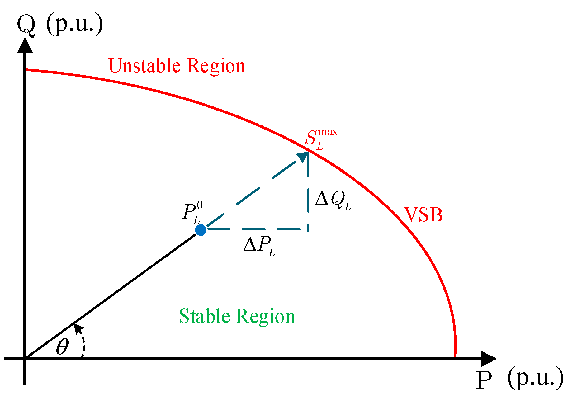
Using the values of , , and , a VSB in a complex load power space, as shown in Figure 8, can be obtained. Such a VSB is able to give system operators a global view of power system voltage stability. The computation process to construct a VSB curve in P-Q plane is given in Algorithm 1.
| Algorithm 1. Construction of a VSB curve in P-Q plane. |
| 1: Input: and ; 2: for do 3: for do 4: ; 5: ; 6: ImpedanceMargin(); 7: PowerMargin(); 8: ; 9: ; 10: ; 11: end for 12: 13: end for 14: Determine by Equation (24); 15: Construct a VSB curve by Equation (23); 16: return VSB curve 17: function ImpedanceMargin() 18: Compute by Equation (7); 19: Compute by Equation (8); 20: ; 21: return 22: end function 23: function PowerMargin() 24: Compute by Equation (22); 25: Compute by Equation (21); 26: return 27: end function |
4. Case Studies
The capability of the proposed algorithm is further demonstrated by utilizing different-size test systems. The system data and the simulation scenarios are listed in Table 1. Two metrics, accuracy and execution time, are utilized to evaluate the performance of the proposed method. Furthermore, its performance is also compared to the CPF method [8] that is widely used in voltage stability assessment. All computations are performed on an Intel® Core™ i5, 1.7 GHz computer.
4.1. Load Change Cases
In this research, extensive simulation studies for load change cases have been performed, including various load levels and various load patterns. Table 2 lists some selected cases, where represents the initial load level, denotes load increases at even load buses, denotes load increases at odd load buses, and denotes load increases at all load buses.
4.1.1. IEEE 14-Bus Model
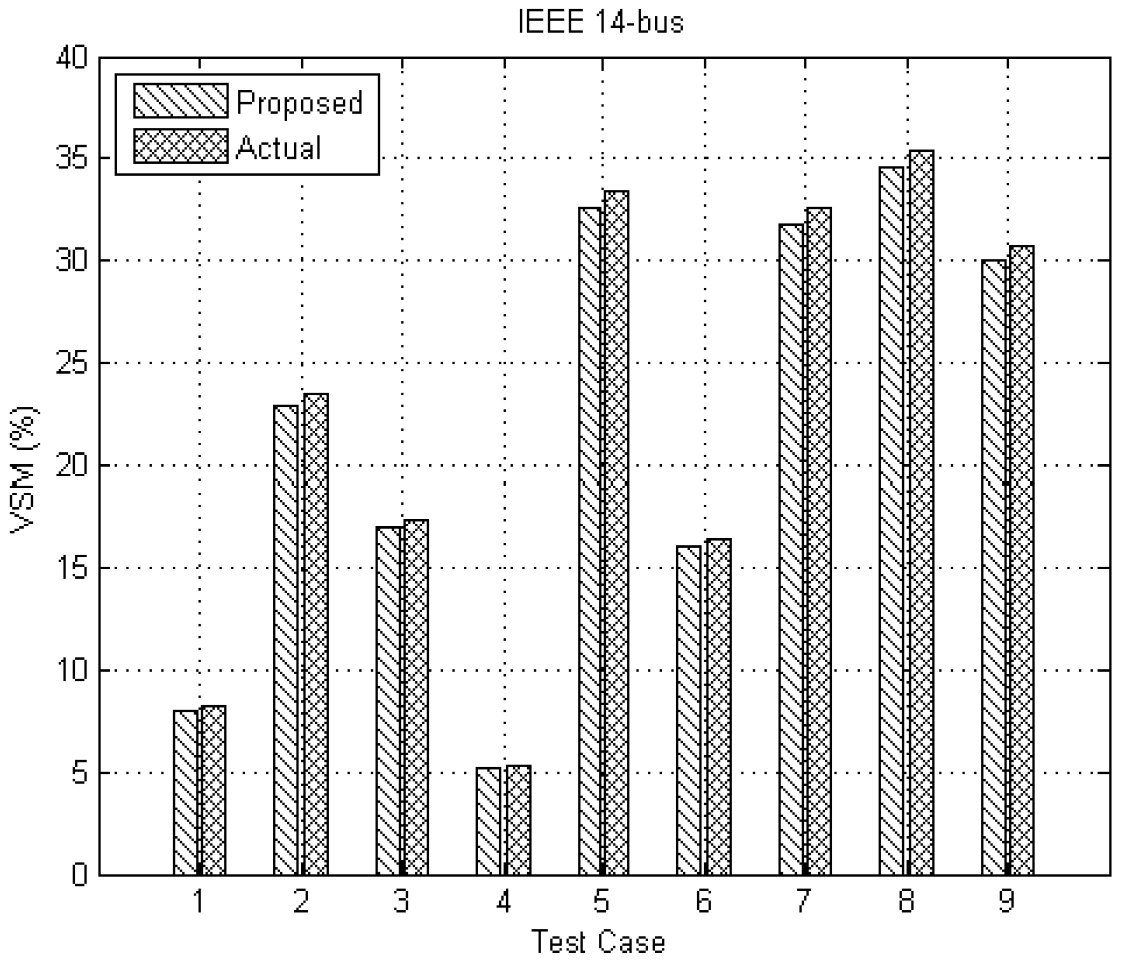
In order to test the algorithm, the IEEE 14-bus model is first utilized. The diagram of the test model is depicted in Figure 9. This model involves 14 buses, 5 generation units, 9 loads, and 20 transmission lines [22].
The results of system VSM estimated by the proposed method under the selected test cases is illustrated in Figure 10, where the values of VSM corresponding to the test cases are depicted on the Y-axis of the figure. From Figure 10, one can see that the estimated VSMs are almost the same as the actual ones.
4.1.2. IEEE 30-Bus Model
4.1.3. Statistical Evaluation
To test the capability of the proposed algorithm for online voltage stability assessment, many simulations were conducted. These include different-size test systems, various load levels, and various load patterns. Among the simulation studies, Table 3 compares the selected results of VSM, along with the execution time for the tested methods. Table 3 shows that the VSMs obtained by the proposed approach get closer to the ones obtained by the CPF approach. However, the proposed approach has less execution time in all cases compared to the CPF approach.
In order to compare the overall efficiency of all the tested methods, an index called the efficiency coefficient (EC) is defined as,
This index combines execution time and accuracy, represented by the VSM based on the given LID. A larger value of EC indicates high efficiency, in terms of less execution time and higher accuracy. Table 3 shows the values of EC for the compared methods. Since a larger system requires more execution time, the value of EC decreases when the system size increases. In addition, Table 3 clearly shows that the proposed approach is significantly more efficient than the conventional CPF approach.
4.2. Topology Change Cases
The aim of this case study is to demonstrate the capability of the proposed method to deal with topology changes in the operating condition. The considered topology change cases include transmission line and generator outages.
Table 4 compares the results in terms of EC for the studied systems. In addition, the table shows several out-of-service cases for each test system. Table 4 shows that the efficiency of the proposed method is significantly higher than the CPF method. Indeed, the proposed method yields results with acceptable accuracy, despite its ease of implementation and low computational cost. Furthermore, we observe, based on extensive simulations carried out, that the proposed method is easily applicable to any power system, regardless of system size and configuration.
4.3. Visualization of VSB in P-Q Plane
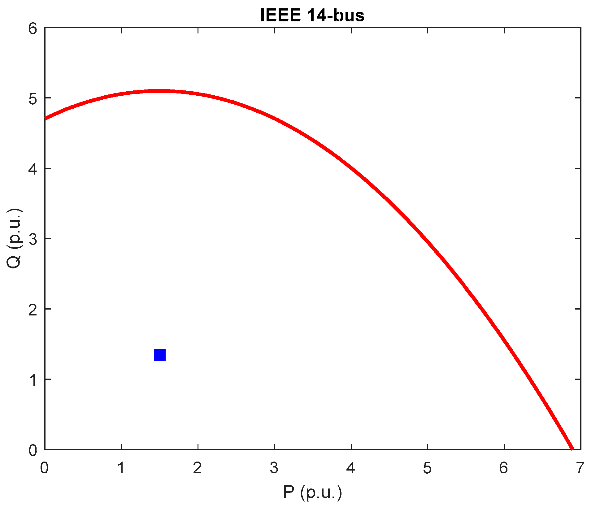
To examine the effects of different look-ahead LIDs on voltage stability assessment, we performed many load patterns on the studied systems. Figure 13 depicts an illustrative case of VSB determination in PQ plane for the IEEE 14-bus model. The maximum transferable load powers (P, Q, and |S|) and the corresponding operating point can be easily identified in Figure 13 (i.e., a VSB curve can give more meaningful information to power engineers). This real-time visualization of voltage stability is achieved via the identification of a VSB curve using PMU measurements.
The criterion used for performance evaluation of VSB approximation is expressed as,
where is defined previously in Equation (25) and denotes the total number of compared points on the VSB. In this study, for each test system. Also note that the exact VSB is computed by point-by-point voltage collapse point computation. Table 5 gives the values of for the compared methods. Through quantitative comparisons with the CPF method, it can be seen that the proposed algorithm is capable of providing acceptable accuracy, but with much less execution time and higher efficiency. This means that a possible VSB, which can improve real-time situational awareness to enhance voltage stability monitoring, can be given quickly by the proposed method.
4.4. Effects of Measurement Inaccuracies
To verify the effects of measurement inaccuracies on VSB determination, we carried out a lot of test cases by simply adding random noise to the original measurements. The total number of compared points on the VSB is set to be 100 for each test system. The results in terms of average error are summarized in Table 6, showing that measurement errors indeed degrade the performance of the VSB determination. However, the issue of data pre-processing can be easily solved by different filtering methods available in studies [23,24].
5. Conclusions
A new PMU-based algorithm for online voltage security monitoring is developed to increase the system operator’s situational awareness for operational decision making. Based on the TE technique and the MT technique for determining loading margin of a transmission grid, the approximation of VSB can be obtained by a quadratic curve using PMU data. Visualization of VSB in a complex load power space gives system operators a global view of power system voltage stability. The proposed algorithm can cope with different kinds of load increase cases. In addition, the algorithm is simple and fast, which makes it adequate for online applications. Numerical test results, using different-size power grid models, illustrate the effectiveness, flexibility, and capability of the proposed algorithm.
Acknowledgments
This work was supported by the Ministry of Science and Technology of Taiwan, under Contract MOST 104-2221-E-035-041 and Contract MOST 106-3113-E-002-012.
Author Contributions
Heng-Yi Su proposed the approach and wrote the manuscript with input from Tzu-Yi Liu.
Conflicts of Interest
The authors declare no conflict of interest.
References
- Andersson, G.; Donalek, P.; Farmer, R.; Hatziargyriou, N.; Kamwa, I.; Kundur, P.; Martins, N.; Paserba, J.; Pourbeik, P.; Sanchez-Gasca, J.; et al. Causes of the 2003 major grid blackouts in north America and Europe, and recommended means to improve system dynamic performance. IEEE Trans. Power Syst. 2005, 20, 1922–1928. [Google Scholar] [CrossRef]
- Simpson-Porco, J.W.; Dörfler, F.; Bullo, F. Voltage collapse in complex power grids. Nat. Commun. 2016. [Google Scholar] [CrossRef] [PubMed]
- Ajjarapu, V. Computational Techniques for Voltage Stability Assessment and Control; Springer-Verlag: New York, NY, USA, 2006. [Google Scholar]
- Su, H.-Y.; Hsu, Y.-L.; Chen, Y.-C. PSO-Based Voltage Control Strategy for Loadability Enhancement in Smart Power Grids. Appl. Sci. 2016, 6, 449. [Google Scholar] [CrossRef]
- Deng, W.; Zhang, B.; Ding, H.; Li, H. Risk-Based Probabilistic Voltage Stability Assessment in Uncertain Power System. Energies 2017, 10, 180. [Google Scholar] [CrossRef]
- Flatabo, N.; Ognedal, R.; Carlsen, T. Voltage stability condition in a power transmission system calculated by sensitivity methods. IEEE Trans. Power Syst. 1990, 5, 1286–1293. [Google Scholar] [CrossRef]
- Flatabo, N.; Fosso, O.; Ognedal, R.; Carlsen, T. A method for calculation of margins to voltage instability applied on the Norwegian system for maintaining required security level. IEEE Trans. Power Syst. 1993, 8, 920–928. [Google Scholar] [CrossRef]
- Ajjarapu, V.; Christy, C. The continuation power flow: A tool for steady state voltage stability analysis. IEEE Trans. Power Syst. 1992, 7, 416–423. [Google Scholar] [CrossRef]
- Chiang, H.D.; Flueck, A.J.; Shah, K.S.; Balu, N. CPFLOW: A practical tool for tracing power system steady-state stationary behavior due to load and generation variations. IEEE Trans. Power Syst. 1995, 10, 623–634. [Google Scholar] [CrossRef]
- Vu, K.; Begovic, M.M.; Novosel, D.; Saha, M.M. Use of local measurements to estimate voltage-stability margin. IEEE Trans. Power Syst. 1999, 14, 1029–1035. [Google Scholar] [CrossRef]
- Smon, I.; Verbic, G.; Gubina, F. Local voltage-stability index using Tllegen’s theorem. IEEE Trans. Power Syst. 2006, 21, 1267–1275. [Google Scholar] [CrossRef]
- Corsi, S.; Taranto, G.N. A real-time voltage instability identification algorithm based on local phasor measurements. IEEE Trans. Power Syst. 2008, 23, 1271–1279. [Google Scholar] [CrossRef]
- Verbic, G.; Gubina, F. A new concept of voltage-collapse protection based on local phasors. IEEE Trans. Power Del. 2004, 19, 576–581. [Google Scholar] [CrossRef]
- Parniani, M.; Vanouni, M. A fast local index for online estimation of closeness to loadability limit. IEEE Trans. Power Syst. 2010, 25, 584–585. [Google Scholar] [CrossRef]
- Sun, T.; Li, Z.; Rong, S.; Lu, J.; Li, W. Effect of Load Change on the Thevenin Equivalent Impedance of Power System. Energies 2017, 10, 330. [Google Scholar] [CrossRef]
- Phadke, A.G.; Thorp, J.S. Synchronized Phasor Measurements and Their Applications; Springer-Verlag: New York, NY, USA, 2008. [Google Scholar]
- Aminifar, F.; Fotuhi-Firuzabad, M.; Safdarian, A.; Davoudi, A.; Shahidehpour, M. Synchrophasor measurement technology in power systems: Panorama and state-of-the-art. IEEE Access 2014, 2, 1607–1628. [Google Scholar] [CrossRef]
- Martin, K.E. Synchrophasor standards development-IEEE C37.118 & IEC 61850. In Proceedings of the 44th Hawaii International Conference on System Sciences, Kauai, HI, USA, 4–7 January 2011; pp. 1–8. [Google Scholar]
- Dubrovin, B.A.; Fomenko, A.T.; Novikov, S.P. Modern Geometry-Methods and Applications; Springer-Verlag: New York, NY, USA, 1984. [Google Scholar]
- Taylor, C.W. Power System Voltage Stability; McGraw-Hill: New York, NY, USA, 1994. [Google Scholar]
- Van Cutsem, T.; Vournas, C. Voltage Stability of Electric Power Systems; Kluwer: Norwell, MA, USA, 1998. [Google Scholar]
- Power Systems Test Case Archive, University of Washington College of Engineering. Available online: http://www.ee.washington.edu/re-serach/pstcal/ (accessed on 14 April 2017).
- Tate, J.E.; Van, Cutsem T. Extracting steady state values from phasor measurement unit data using FIR and median filters. In Proceedings of the 2009 IEEE/PES Power Systems Conference and Exposition, Seattle, WA, USA, 15–18 March 2009; pp. 1–6. [Google Scholar]
- Glavic, M.; Van Cutsem, T. Wide-area detection of voltage instability from synchronized phasor measurements, part I: Principle. IEEE Trans. Power Syst. 2009, 24, 1408–1416. [Google Scholar] [CrossRef]
Figure 1.
Illustration of phasor measurement unit (PMU)–based wide-area monitoring system (WAMS) in a smart grid.
Figure 1.
Illustration of phasor measurement unit (PMU)–based wide-area monitoring system (WAMS) in a smart grid.

Figure 2.
Thevenin equivalent (TE) network for a power system seen at a load bus.

Figure 3.
Illustration of the impedance match method for voltage stability monitoring.
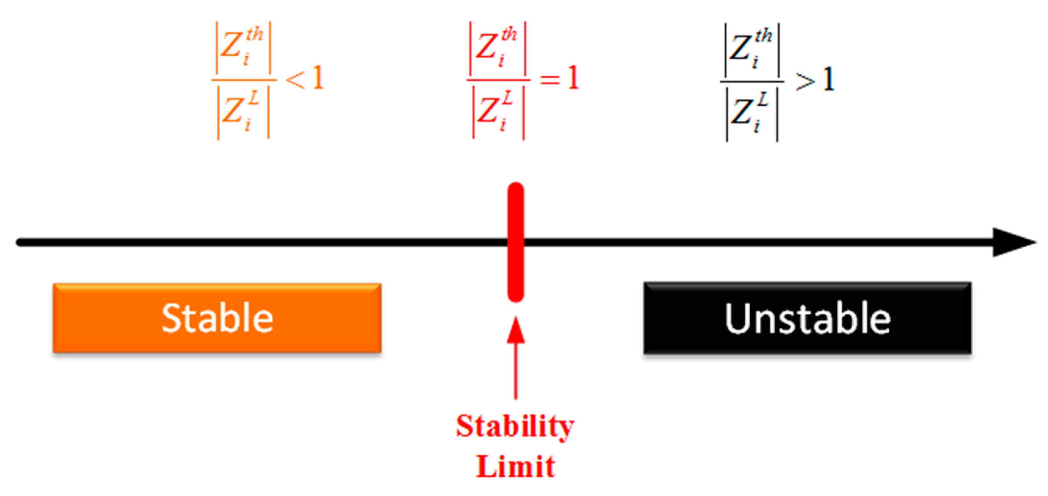
Figure 4.
Main steps in the proposed algorithm for voltage stability visualization and monitoring.
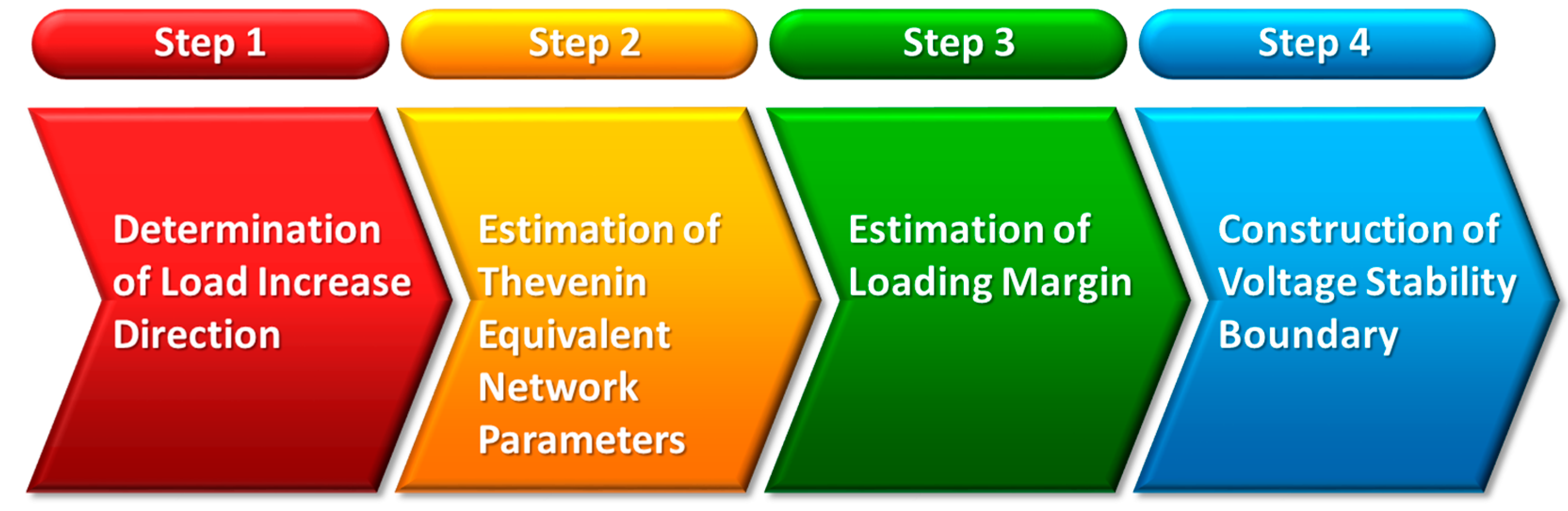
Figure 5.
Load power parameter space.
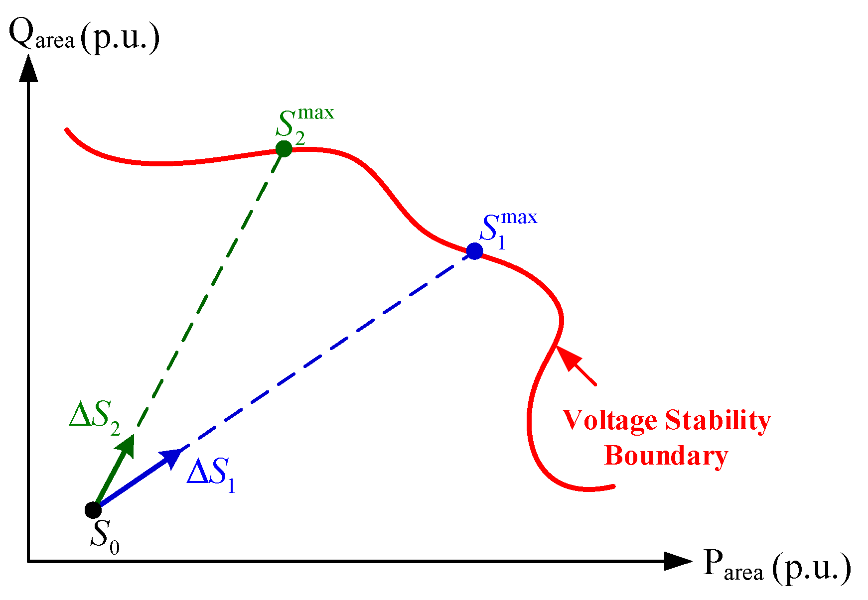
Figure 6.
Trajectory of and as increases.
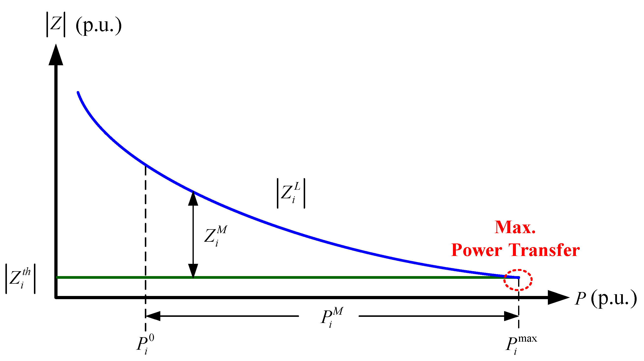
Figure 7.
Illustration of the transformation between and .
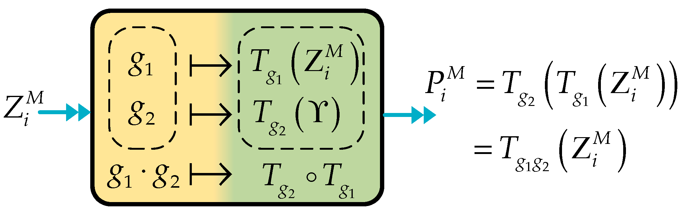
Figure 8.
Voltage stability boundary (VSB) in a complex load power space.

Figure 9.
IEEE 14-bus test system.
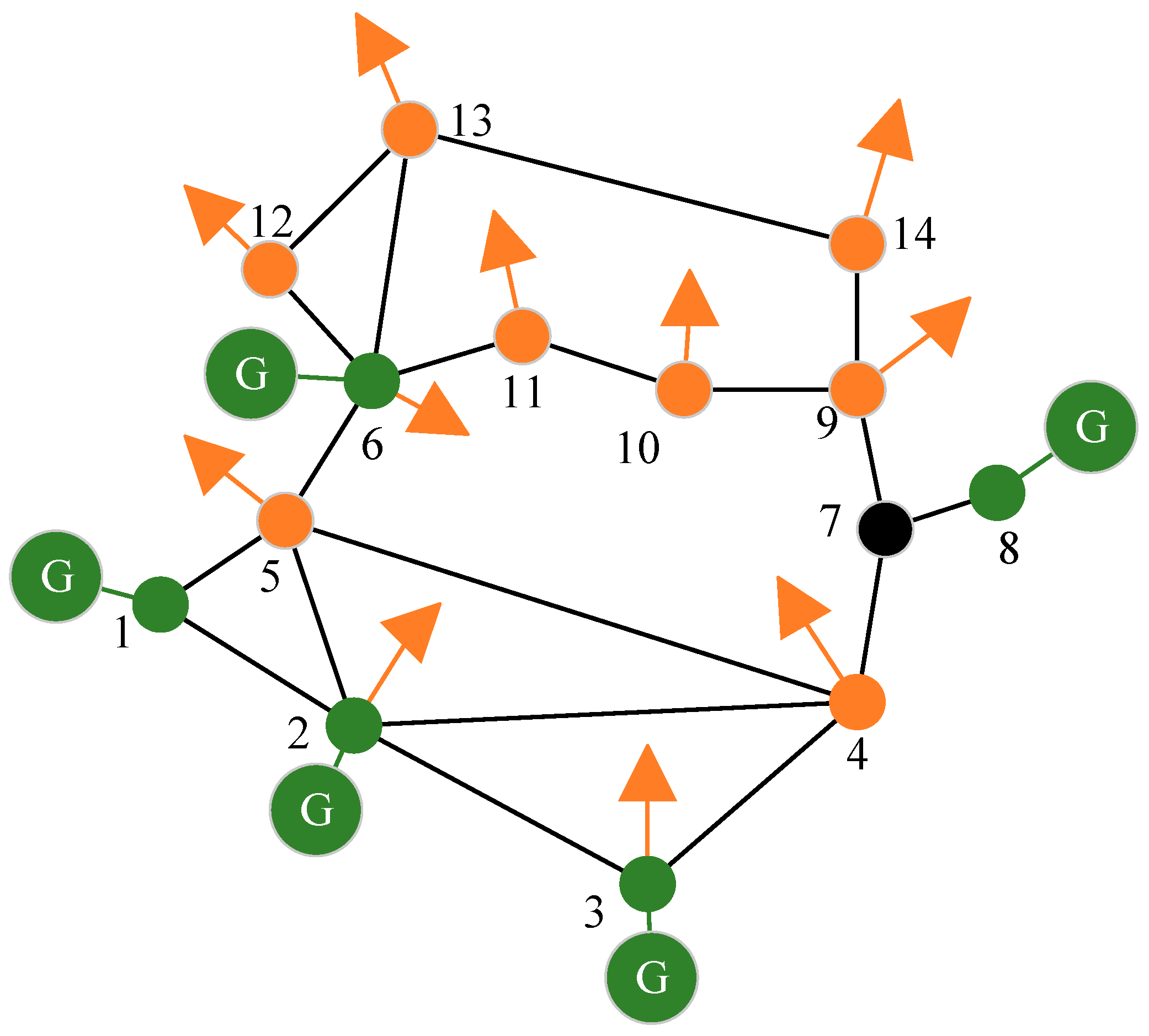
Figure 10.
Estimation of system VSM for IEEE 14-bus model.

Figure 11.
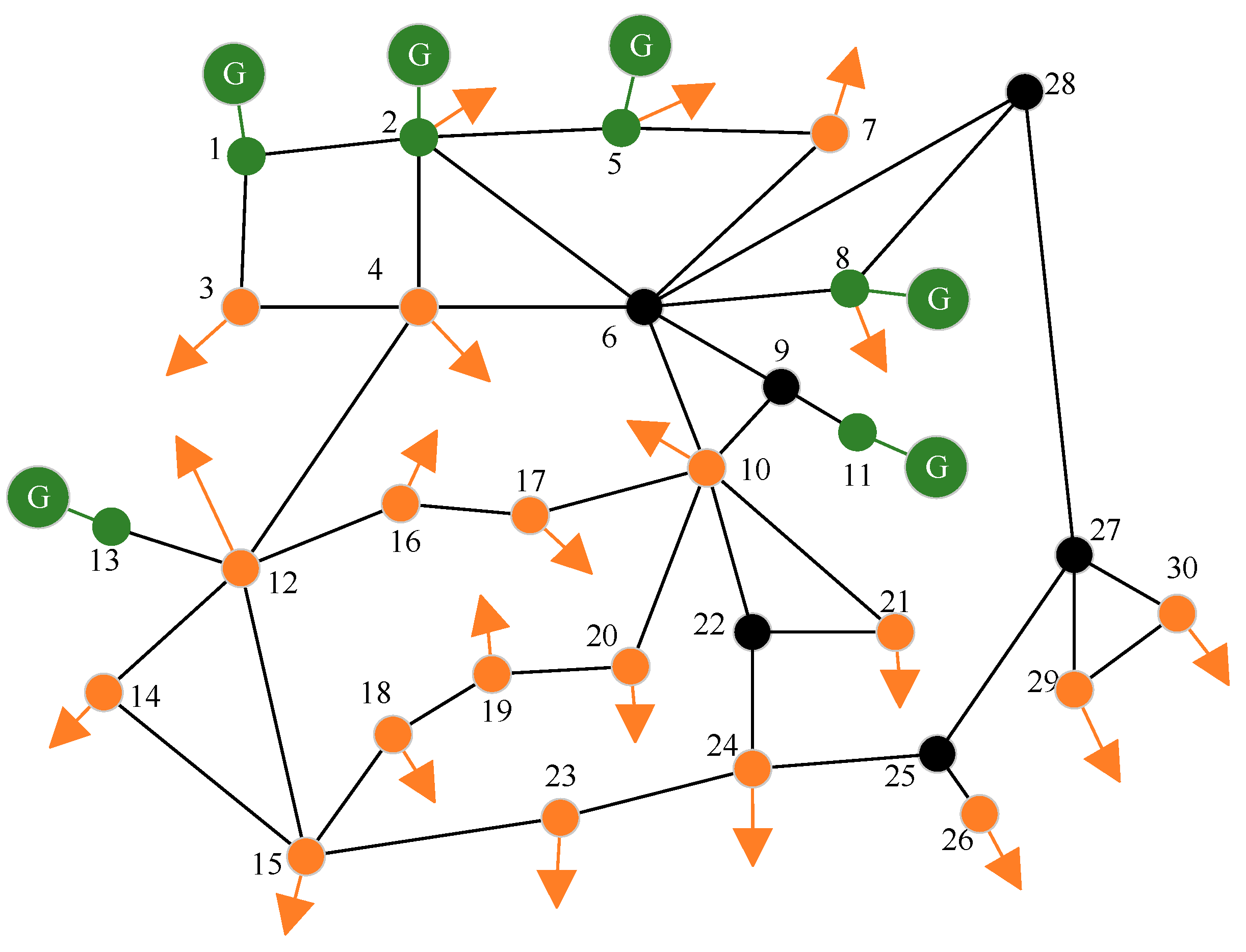
IEEE 30-bus test system.

Figure 12.
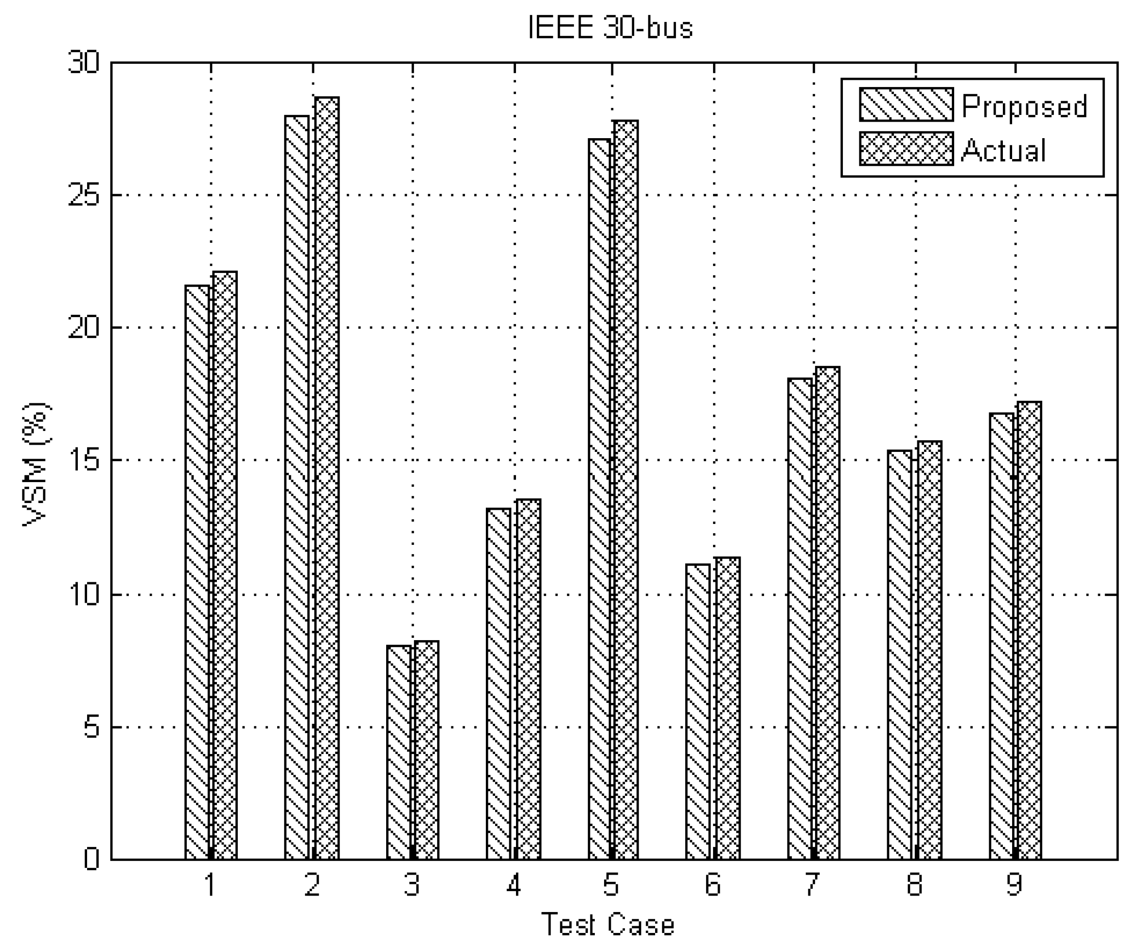
Estimation of system VSM for IEEE 30-bus model.

Figure 13.
VSB in P-Q plane for IEEE 14-bus model. The point at (1.5, 1.35) is the initial operating point.
Figure 13.
VSB in P-Q plane for IEEE 14-bus model. The point at (1.5, 1.35) is the initial operating point.


Table 1.
System data and the simulation scenarios.
| Number of | IEEE 14-Bus | IEEE 30-Bus | IEEE 57-Bus | IEEE 118-Bus | IEEE 300-Bus |
|---|---|---|---|---|---|
| Generators | 5 | 6 | 7 | 54 | 69 |
| Loads | 9 | 24 | 50 | 64 | 231 |
| Lines | 20 | 41 | 80 | 186 | 411 |
| Scenario | Description | ||||
| Load change | Various load levels together with various load patterns | ||||
| Topology change | Transmission line and generator outages | ||||
Table 2.
Selected load increase cases.
| Case | Load Level | Load Pattern |
|---|---|---|
| 1 | ||
| 2 | ||
| 3 | ||
| 4 | ||
| 5 | ||
| 6 | ||
| 7 | ||
| 8 | ||
| 9 |
Table 3.
Comparison of the results for the considered test systems in load change cases.
| Test System | VSM (%) | Time (s) | EC | |||
|---|---|---|---|---|---|---|
| Proposed | CPF | Proposed | CPF | Proposed | CPF | |
| IEEE 14-bus | 22.17 | 22.48 | 0.25 | 1.36 | 5.38 | 0.99 |
| IEEE 30-bus | 34.01 | 34.63 | 0.41 | 2.59 | 3.74 | 0.59 |
| IEEE 57-bus | 17.57 | 17.96 | 1.06 | 6.04 | 1.17 | 0.21 |
| IEEE 118-bus | 9.06 | 9.41 | 1.62 | 10.34 | 0.59 | 0.09 |
| IEEE 300-bus | 12.94 | 13.27 | 12.44 | 73.42 | 0.09 | 0.02 |
Table 4.
Comparison of the results for the considered test systems in topology change cases.
| Test System | Out of Service | EC | |
|---|---|---|---|
| Proposed | CPF | ||
| IEEE 14-bus | Line 9–10 | 5.25 | 1.36 |
| Line 12–13 | 4.94 | 0.98 | |
| G2 | 5.03 | 1.01 | |
| IEEE 30-bus | Line 21–22 | 3.68 | 0.63 |
| Line 10–17 | 3.31 | 0.47 | |
| G13 | 3.97 | 0.72 | |
| IEEE 57-bus | Line 23–24 | 1.78 | 0.59 |
| Line 9–55 | 1.04 | 0.15 | |
| G8 | 1.36 | 0.34 | |
| IEEE 118-bus | Line 18–19 | 0.63 | 0.19 |
| Line 63–64 | 0.58 | 0.11 | |
| G24 | 0.60 | 0.14 | |
| IEEE 300-bus | Line 11–13 | 0.14 | 0.05 |
| Line 15–37 | 0.08 | 0.02 | |
| G10 | 0.11 | 0.04 | |
Table 5.
Comparison of the results in terms of ECavg for the considered test systems.
| Test System | ||
|---|---|---|
| Proposed | CPF | |
| IEEE 14-bus | 5.07 | 1.12 |
| IEEE 30-bus | 3.65 | 0.64 |
| IEEE 57-bus | 1.39 | 0.37 |
| IEEE 118-bus | 0.61 | 0.15 |
| IEEE 300-bus | 0.12 | 0.04 |
Table 6.
Effects of measurement errors to VSB determination.
| Test System | Error (%) | |
|---|---|---|
| No Measurement Errors | With Measurement Errors | |
| IEEE 14-bus | −1.56 | −4.66 |
| IEEE 30-bus | −2.05 | −5.24 |
| IEEE 57-bus | −1.79 | −4.98 |
| IEEE 118-bus | −2.46 | −5.47 |
| IEEE 300-bus | −2.34 | −5.31 |
© 2017 by the authors. Licensee MDPI, Basel, Switzerland. This article is an open access article distributed under the terms and conditions of the Creative Commons Attribution (CC BY) license (http://creativecommons.org/licenses/by/4.0/).
Share and Cite
MDPI and ACS Style
Su, H.-Y.; Liu, T.-Y. A PMU-Based Method for Smart Transmission Grid Voltage Security Visualization and Monitoring. Energies 2017, 10, 1103. https://doi.org/10.3390/en10081103
AMA Style
Su H-Y, Liu T-Y. A PMU-Based Method for Smart Transmission Grid Voltage Security Visualization and Monitoring. Energies. 2017; 10(8):1103. https://doi.org/10.3390/en10081103
Chicago/Turabian StyleSu, Heng-Yi, and Tzu-Yi Liu. 2017. "A PMU-Based Method for Smart Transmission Grid Voltage Security Visualization and Monitoring" Energies 10, no. 8: 1103. https://doi.org/10.3390/en10081103
Note that from the first issue of 2016, this journal uses article numbers instead of page numbers. See further details here.