
Assessment of Credible Capacity for Intermittent Distributed Energy Resources in Active Distribution Network


1
Key Laboratory of Control of Power Transmission and Conversion, Ministry of Education, Department of Electrical Engineering, Shanghai Jiao Tong University, Shanghai 200240, China
2
Electric Power Research Institute of Guangdong Power Grid Corporation, Guangzhou 510080, China
*
Author to whom correspondence should be addressed.
Energies 2017, 10(8), 1104; https://doi.org/10.3390/en10081104
Submission received: 26 April 2017
/
Revised: 29 June 2017
/
Accepted: 24 July 2017
/
Published: 27 July 2017
(This article belongs to the Special Issue Innovative Methods for Smart Grids Planning and Management)
Abstract
:The irregularity and randomness of distributed energy sources’ (DERs) output power characteristic usually brings difficulties for grid analysis. In order to reliably and deterministically evaluate intermittent distributed generation’s active power output, a credible capacity index for active distribution network (ADN) is proposed. According to the definition, it is a certain interval that the stochastic active power output of DERs may fall in with larger probability in all kinds of possible dynamic and time varying operation scenarios. Based on the description and analysis on the time varying scenarios, multiple scenarios considered dynamic power flow method for and are proposed. The method to calculate and evaluate credible capacity based on dynamic power flow (DPF) result is illustrated. A study case of an active distribution network with DERs integrated and containing 32 nodes is selected; multiple operation scenarios with various fractal dimension are established and used. Results of calculated credible capacity based on several groups of scenarios have been analyzed, giving the variance analysis of groups of credible capacity values. A deterministic value with the maximum occurrence probability representing credible capacity is given. Based on the same network case, an application of credible capacity to grid extension planning is given, which contributes to expenditure and cost reduction. The effectiveness and significance of the proposed credible capacity and solution method have been demonstrated and verified.
1. Introduction
As the best substitution of fossil fuels, a fast growth of renewable energy to supply the global energy demand has been developed worldwide in the past decades. Impacts of renewable energy based distributed generation (DG) on the electric power grid appear to be obvious with its massive application of integration [1,2]. A great number of studies considering this issue are emerging, which manage to analyze the impact quantitatively [2,3], statistically figure out the irregularity of intermittency and fluctuations, and predict and estimate future output in various ways [4,5]. Current literature can also be found investigating other domains such as grid planning [6,7,8,9], operation analysis, and optimization control considering the uncertainties of DG [10,11,12,13,14,15,16]. A power supply and storage capacity for operation optimization is proposed and studied [17]. Basically, these existing questions have much to do with the unique output power characteristics of DG that tell it apart from other conventional power resources. Descriptions, analysis of the characteristics of DG’s output power and modeling lay a foundation for further research. Thus, this becomes one of the most important and fundamental tasks that need to be profoundly studied.
Statistics and probability methods are the most commonly adopted tools to evaluate and assess the fluctuations and variations of DG’s output power, which usually necessitates large quantities of analysis based on long term historical data and even meteorological information records. Wind power resources and measurement data of nearly half a century in some European countries were collected and summarized for technical characteristic analysis to come up with future development suggestions [18,19]. Reference [20] systematically classified a group of statistical indexes of wind power, and built a wind power characteristic evaluation index system. It includes variation rate of wind output power, randomness indexes and several operational indexes. It also analyzed the application of indexes in different spatial and temporal scales with considerations of integration problems. Reference [21] defined and specified fluctuation rates of all integrated DG’s output power, which is subjected to the selected time interval and correlations of power resources. Besides, based on a large number of field measurements, a t location-scale distribution approach is proposed and verified suitable to identify the probability distribution of wind power variations in minutes’ level [22]. Reference [23] proposed a recurrence plot and the recurrence rate based on phase space reconstruction to qualitatively and quantitatively depict the volatility. It can be used to analyze the relationship between the volatility of a wind power sequence and prediction errors. However, existing statistical indexes and developed probability models are still far from adequate for use [24].
As for operation analysis with characteristics of DG’s output power, multiple types of stochastic variables distribution and fuzzy functions are widely used in power flow calculation [25,26,27,28]. Based on power flow results, key technical indexes such as voltage distribution, probability of limitation violations, power losses, and system reliability can be achieved. However, this greatly depends on the accuracy of the probability or stochastic variable model, which describes the output power characteristics. It is always a difficult task to eliminate errors comparing with real measurement data. On the other hand, deterministic power flow methods considering dynamic and stochastic variations in continuous time period have also been studied. These studies are commonly seen in optimal power flow, which achieved a comprehensive optimal goal under various dynamic scenarios with the constraints of grid and controllable devices limitations. In multiple dynamic operation scenarios with wind power and energy storage integrated, reference [29] proposed an objective function aiming at maximizing equivalent export power and benefit of distribution grid, which obtained an optimal power flow distribution covering multiple time periods. Reference [30] proposed an optimal schedule aiming at minimizing the total operational costs and emissions while considering the intermittency.
Distribution network planning issue considering the uncertainties of distribution generations usually pertains to the description and modeling of uncertainties and stochasticity of intermittent energy resource. Reference [31] established stochastic wind speed and load model, incorporating the model in the proposed multi-configuration multi-scenario market-based optimal power flow, to achieve satisfied active distribution networks planning solution. Based on a large amount of historical data analysis, stochastic output is abstracted into multiple scenarios with their probability of occurrence, and then substituted it into multi-objective planning model [32,33]. Reference [34] put forward a dynamic fuzzy interactive approach for expansion planning in a long term period.
It is undeniable that the extreme irregularity of the output of intermittent power resource usually makes it difficult to predict and estimate with a high precision. Obviously, there is little possibility to explore and establish a perfect math model. Therefore, these reported methods are by far still incapable of precisely defining the intrinsic attribute of DG’s intermittency, and solve related problems in operation analysis and grid planning domain.
A concept of credible capacity of intermittent energy resources came into academia’s view in recent years. Reference [35] explained the physical meaning which refers to the conventional generation units’ capacity that can be replaced by wind power under the same system reliability level in bulk power systems. This is a deterministic value that represents stochastic energy resource’s power support and reliability impact on the system. Therefore, this concept and its application make it more feasible for grid analysis and optimal decision making, when incorporating irregularities and fluctuations. Multiple numerical methods to calculate the index were investigated and explored. According to the literature, there are several ways to adopt the Monte-Carlo simulation, sequence operation theory and stochastic production simulation to calculate the index with different computation efficiency [36,37,38,39]. Related research on capacity credit assessment of a hybrid generation system composed of wind farm, energy storage system and photovoltaic system has been given, which analyzed complementary benefits [40]. These studies are all based on statistical analysis of wind power’s historic data and feature abstraction. The calculation of credible capacity can thus be enabled, which can crucially contribute to better analyze and solve the problems mentioned above.
In this work, a novel credible capacity index is defined and proposed to reliably estimate and evaluate the actual active power output of all distributed energy resources (DER), which is introduced in Section 2. Indicators reflecting the variations of intermittent energy resources are established to describe and analyze time-varying operation scenarios. According to state combinations of indicators and the corresponding meaning it reveals, output model of controllable devices is proposed to balance power disturbances, which is discussed in Section 3. Based on the description of dynamic and time-varying scenario, a multi-scenario considered dynamic power flow method is introduced for the calculation of credible capacity, which is addressed in Section 4. Groups of credible capacity values are evaluated based on several actual dynamic operation scenarios and case network in Section 5. Moreover, the feasibility is demonstrated and verified.
2. Definition of Credible Capacity and Its Physical Meaning
For operation analysis issue of power grid integrating DERs, the proposal of credible capacity and its application in current research makes it easier to deterministically and quantitatively describe intermittent power resource’s unpredictable randomness to bring much convenience to further analysis research. On the other hand, irregular and non-differentiable complicated geometry graphics remain self-similar in the same scale-free interval, according to fractal theory [41,42]. It means that the fluctuations of intermittent energy resources can also be quantitatively analyzed. Fractal theory based applications in electric power system are mainly seen in stochastic load sequence modeling and forecasting [43,44,45]. Thus, for active distribution network, in which the uncertainty and stochasticity are much more prominent, further investigation should be made.
In this work, dynamic operation scenario refers to stochastic output of intermittent power resources under steady state. The power injection variations lead to operation scenario variations. A novel credible capacity index mainly for ADN is proposed, which differs from concept and definition to former research. From physical perspective, credible capacity is a deterministic value or a certain interval reflecting the active power output of all DERs including controllable and intermittent power resources in a coordinated way of operation. Therefore, the value of credible capacity is determined by multiple operation scenarios, and is also substantially subjected to the electric parameters of DERs and network, regardless of the extreme irregularity and stochasticity.
The definition of credible capacity is given below. Numerically, this index refers to a particular value that the output of all DERs including intermittent power resource may regularly fluctuate around. More accurately, it is a certain interval of deterministic value that the stochastic active power output of DERs may fall in with a required probability level. As shown in Equation (1), β represents the required probability of the interval which the credible capacity value is in means the set of credible capacity’s value derived from power flow results of multiple dynamic operation scenarios. Symbol inf and sup are the lower and upper limits of the set . f (•) is the probability density function of credible capacity value distributed in this interval in one-dimensional space.
The proposed credible capacity index can be considered as a reliable estimation according to long time scale of actual operations. That is, the ability and effect of a coordinated operation of controllable and intermittent power resources is embedded in this index, which is an intrinsic characteristic of active distribution network. Specifically, the proposed credible capacity of all DERs is derived from a network’s overall view rather than only prediction techniques and analysis utilized for the intermittent distributed generations, which has rarely been clearly discussed before. Thus, it can also be used for grid analysis with more precisions.
Thus, according to the definition, expressions to calculate credible capacity are given below. In a distribution grid with multiple DERs integrated, assume that the network contains n nodes. It is obvious that Equation (2) holds at any time according to system’s active power balancing equations.
In Equation (2), stands for active power injection of slack node at specified time section t. Except for slack node, and stand for the sum of active power output of all DERs and loads at specified time section t, respectively.
From a system’s global view in real time operation combining multiple scenarios, the credible capacity of all DERs integrated can thus be derived and calculated according to the power flow results of a certain specified time period, which is shown below in Equation (3).
Here, means the sum of each load node’s average load active power within a specified time process. Similarly, is the average value of network active power loss, and is the average value of power injection of slack node.
, the sum of each load node’s average load active power within the specified time period of a certain scenario, can be calculated through Equation (4), as given below. The subscript x is used to distinguish between different load power levels at the same node. Thus, means the x-th load power value in this time period at node i, and means the duration time of this load power level. Tp stands for the total time. n represents the total node number of the network.
The network’s total active power loss can be calculated according to Equation (5) in which U represents node voltage and θ is phase angle. Ui stands for voltage amplitude at node i, n for the total node number of network, Gij for the conductance of branch line ij, θij for phase angle difference of node i and j.
Surely, it is also time-varying. Thus, the average value of network active power loss can be calculated through Equation (6), as shown below. T represents the length of studied time period of selected operation scenario.
stands for the average value of power injection of the slack node in the studied time period of a certain scenario. The overall electric energy that the slack node injected into the grid is divided by the total time as shown in Equation (7).
Thus, credible capacity of all DERs in the network can be figured out by substituting Equations (4), (6) and (7) into Equation (3).
The proposed credible capacity can be used to assess and evaluate the active power of intermittent DERs in ADN according to the above illustrated definition and explanation. However, in such stochastic and time-varying operation scenarios, how a credible capacity index can be calculated for better evaluation becomes a crucial problem. Although it can be directly calculated by statistical analysis on real time measuring data, more effective analytic tools rather than conventional methods should be adopted.
Dynamic power flow (DPF) method considering multiple dynamic scenarios, which is mainly used for tracking the grid’s dynamic operation trajectory within a continuous time period, can better reflect the system’s real time status compared to conventional methods when tackling with uncertainties and stochasticity. Thus, based on the description and analysis of time-varying operation scenarios, a novel dynamic power flow method considering multiple scenarios is proposed and adopted for the calculation and evaluation of credible capacity. Namely, based on the DPF results of several dynamic scenarios reflecting the variations of ADN in a specified continuous time period, key variables of Equations (4)–(7) can thus be statistically calculated. The value of credible capacity is valid to some extent representing its true value corresponding to each scenario. By using relevant numerical methods, such as statistics and interval distribution probability, to analyze groups of data derived from DPF results of different scenarios, it is feasible to evaluate the credible capacity’s final value of all DERs including the intermittent power resources.
3. Analysis on the Time Varying Operation Scenario
3.1. Tracking Indicator and What it Reveals
The variations of the operation scenario should be described and reflected in an active distribution gird with wind turbine and energy storage system (ESS) integrated. Although it is difficult to predict the output due to the strong randomness and uncertainty, the application of techniques such as variable pitch angle control ensures that the active power output will not change sharply in very short time scales. Appropriate tracking indicator should be established.
Exponential Moving Average (EMA) index is widely used in stock market to indicate the variation trend of stochastic unpredictable stock prices. This statistical index is adopted in this work to reflect the mid-term trend of numerical changes and movements in wind power output. For any single wind power turbine, the definition of EMA indicator is shown below in Equation (8).
Here, t means time stamp corresponding with
values on EMA curves at this time. σ stands for
smooth factor that varies from different time scales. It can be calculated
through Equation (9) as given below. represents the current output power of wind power.
The EMA indicator relatively smoothly reflects the fluctuations and changes of wind power in the period T. The value of T may have different options to study the changing trend of the object variable in different time scales, either long or short.
Define two EMA lines with the period of 10 s and 30 s, respectively. With such parameter configuration of time period T, the corresponding smooth factors are 0.1818 and 0.0645, which are calculated through Equation (9). The assignment of T = 10 and T = 30 with the two smooth factors are appropriate to timely assess wind power variations, and reflect as many details as possible within the scope of analytic and computational capability of the proposed methodology. Thus, the difference DIF of the two EMA lines’ values at the same time is shown below in Equation (10).
Therefore, the value of DIF equals to the value of EMA line with period of 10 s minus that of 30 s. The positive and negative of the DIF value itself and the slope of its tangent form different state combinations, which reflect the variations of stochastic and intermittent wind power output, as shown in Figure 1. The fluctuations and changes that cause transitions between different states are also indicated in Figure 1.
When the value of DIF is greater than zero, if holds, current wind power output is demonstrated to be in a monotone increasing trend or otherwise in an interval. When the value of DIF becomes smaller than zero, if holds, it means the wind power output is currently in a monotone decreasing trend. Otherwise, it is in an interval if holds. These different combinations represent four major operation states between which transitions can happen, which will contribute to analyze the time varying operation scenario.
Besides, to improve the stability of wind power’s output, ESS is also required to adjust its output flexibly and continuously changes according to the variations of wind power based on these indicators.
3.2. ESS Adjustment in Accordance with Stochastic Wind Power Output
Controllable ESS provides active power support for the network. Adjustments in accordance with intermittent power resource can contribute to a coordinated operation. Namely, the active power output of ESS is a continuous variable. It responds to wind power fluctuations and balances the disturbances by appropriate adjusting and control. A simple piecewise linear model is adopted, which is given below in Equation (11).
Here, t means continuous time, P(t0) stands for the initial value and k for the slope of each line segment. PESS(t) represents the real time active power output of ESS. Numerically, positive stands for discharging and negative for charging.
To avoid long distance transmission of power and reduce network losses, it is allowed to allocate disturbances of intermittent power resource to the ESS with the minimum electrical distance to stabilize power fluctuations. Generally, it is essential to obtain the grid’s power flow and the data of wind power output at the initial moment, which is under a steady state. The piecewise linear model given in Equation (11) is determined by the following circumstances.
- If both the value of DIF and the slope of its tangent are positive, assign the negative value of the slope of the DIF tangent to the variable k in Equation (11) as the slope of a new line segment. ESS’s initial value P(t0) of this new line segment equals to the difference of wind power’s output before the state of tracking indicators changes and current output active power.
- If both the value of DIF and the slope of its tangent are negative, assign the absolute value of the slope of the DIF tangent to the variable k in Equation (11) as the slope of a new line segment. ESS’s initial value P(t0) equals to the difference of wind power’s output before the state of tracking indicators changes and current output active power.
- If the value of the product of DIF multiplied by the slope of its tangent is negative, ESS’s output remains constant and identical to its output before the value of DIF or the slope of its tangent changes.
That is the strategy of how ESS reacts to the variations of unpredictable stochastic power resources. Therefore, ESS devices have different outputs corresponding to each state, as shown in Figure 1. If any transition occurs between the four states, ESS’s output changes immediately. Figure 2 illustrates this mechanism, in which a simple cosine function is chosen as an example to represent DIF curves.
It also has to meet constraints such as capacity, limitations of charging and discharging rates. Besides, the following inequality constraints must be satisfied at all times. and stand for charging and discharging rate. is the remaining capacity of the ith ESS at specified time t.
In addition, the duration of the ESS maintaining a certain state is limited. If the capacity of ESS no longer supports its adjustment strategy according to current variations of tracking indicators, it should quit operation or adjust its output in the opposite direction. This piecewise linear model, which represents the continuous variations of scenarios and ESS’s reaction to it, can thus be applied to dynamic power flow model considering multiple scenarios for further analysis.
4. Multi-Scenarios Considered Dynamic Power Flow and Its Solution to Calculate Credible Capacity
Based on the time-varying linear model describing ESS’s output, a dynamic power flow method for active distribution network is proposed. Generally, dynamic power flow for transmission network has been commonly studied and applied in power and frequency coordinated adjustment between generation units when large disturbances occur. Different from that of transmission network, the proposed DPF method for ADN, under uncertain conditions in continuous time period, is essentially about system’s operation trajectory tracking and analyzing the gradual changing of system’s power flow distribution. Deterministic power flow results can be obtained by utilizing the proposed DPF method considering stochastic continuous variations of DERs. Therefore, a more accurate analysis of grid’s status and characteristics can be derived. Based on DPF results, the value of credible capacity of DERs including intermittent wind power can be quantitatively estimated.
To evaluate credible capacity of DERs through DPF calculation, multiple operation scenarios have to be considered to cover as many stochastic variation situations as possible. As mentioned above, stochastic and continuous power injection of intermittent power resource leads to ADN’s operation scenario variations under steady state. Dynamic operation scenario refers to all kinds of possible stochastic output of intermittent power resources. Irregular curves of output power of DERs share the similar fractal dimension in the same scale-free interval, according to fractal theory. Therefore, these dynamic operation scenarios are distinguished and categorized by the fractal dimension, namely the quantified irregularity of the curves of intermittent power injected.
Therefore, the multi-scenarios considered DPF method should be rapid in tracking random power fluctuations in real-time and continuously adjusts the output of ESS to allocates possible random disturbances. Rapid iteration is also needed to solve the DPF model. Formally, model of the multi-scenarios considered DPF method and its solutions are elaborated below.
Real time measurement data of load’s active and reactive power, together with wind active power, can be taken into the node power imbalance equations as expressed in Equation (14).
Here, stands for wind active power at node i. and stand for load’s active and reactive power. is the output of ESS which is defined in Equation (11). The slack node of the system is excluded in Equation (14). U stands for node voltage amplitude. stands for the reactive power output of asynchronous wind generator, which is considered as PQV node that the node voltage must be maintained to a certain stable level while its active and reactive power are given. It depends on node voltage, inherent parameters and active power. It is determined by Equations (15) and (16).
Here, is active power output, stands for power factor. R for rotor resistance, Xm for exciter reactance, and for the sum of stator reactance and rotor reactance. Slip ratio s can be determined by Equation (16). Due to the limitation of total penetration rate, there is less occurrence possibility of massive reactive power deviation and voltage instability compared with transmission network. Auxiliary measures of voltage regulation and reactive power compensation can also improve the voltage quality. Thus, the DPF method here neglects voltage issues.
Therefore, the multi-scenarios considered DPF model is given above. The classical Newton-Raphson method can be used. However, it is too complicated to calculate the partial derivative of the voltage amplitude of wind power integrated node. PQV node is considered as normal PQ node when solving the multi-scenarios considered DPF model and neglects the relation between node voltage and reactive power of wind power. Thus, the Jacobian matrix is identical to the traditional Newton-Raphson method.
Since voltage difference of adjacent nodes is small in distribution network, and very few grounding branches exist, the Jacobian matrix is simplified by omitting sinusoidal components in the matrix, as shown in Equation (17).
The total network active power loss can be calculated according to Equation (5) with the obtained node voltages and phase angles after each iteration.
The solving of power loss of large number of branches and accumulation cost many computational resources, making the calculation process of Equation (5) too complex. A simplified solution to active power loss is developed.
According to the DPF result, the system moves to new steady point each time in a continuous time process. Thus, the discrete sequence of each node’s voltage and phase angle can be derived as well as the amount of changes compared to the last balanced state.
For the system’s state variables of node voltage and phase angle that are to be calculated by DPF, set and . Substitute and into Equation (5) to replace and , and then expand Taylor series of Equation (5) at point and , omitting two order and higher terms. Equation (18) can be achieved.
Here, and stand for change quantity of each node’s voltage and phase angle compared to the last balance state, rather than each step of corrections in the power flow iteration equation. The power loss factor vector can be achieved by calculating Equation (19).
The difference of angles between adjacent nodes in distribution network is usually very small. The value of in Equation (19) is considered zero. Thus, the network power loss of the next steady state can be achieved by Equation (20), avoiding a large number of cumulative operations.
Thus, based on the classical Newton–Raphson method, simplified Jacobian matrix and improved way to calculate system’s active power loss are adopted to solve the multi-scenarios considered DPF model.
The proposed multi-scenarios considered DPF method is crucial to the credible capacity index. Thus, the algorithm has to be robust enough and follow the possible rapid changes of variables in every step of computation and iteration. Simplified Jacobi matrix and improved method to calculated system’s active power loss are used to meet the requirements of online analysis.
Besides, the network loss variation between two adjacent steady states is given below in Equation (21), according to Equation (20).
Thus, the system’s overall active loss variation that the system reaches a steady state each time can be calculated. This forms a discrete numeric sequence. Statistical analysis can be made on this sequence of system active power loss variations, and variations’ average value can be statistically calculated. Therefore, , the average value of network’s active power loss, can be calculated through Equation (22), in which means the network active loss at the initial steady state. This significantly simplifies the computing complexity of Equation (6) and contributes to the calculation of credible capacity.
In summary, by utilizing the proposed tracking factors and the DPF method, system’s power flow in a continuous time period can be obtained reflecting the system operation in stochastic dynamic scenarios. Credible capacity index reliably estimating output of DERs can also be evaluated.
Therefore, it can be concluded that the credible capacity index has much to do with the practical operation and depends on the operation scenarios which is crucially important. Different operation scenarios may result to quite different values of credible capacity. Thus, based on abundant basic operation scenarios and wind power background data, the value of credible capacity index can be accurate enough to represent its true value.
5. Case Study
An ADN case at a voltage level of 10 kV is selected. The network consists of four feeders that origin from three substations. There exists up to six interconnection switches, as shown in Figure 3.
The case network contains 32 nodes, 26 loads and with several DERs integrated. In Figure 3, numbered “WG” represents distributed wind generators with small capacity. ESSs all refer to sodium-sulfhur battery (NAS) energy storage systems in this work, and are generally connected to critical grid nodes with heavy loads, intermittent power resources and of high node betweenness. Since instantaneous active power adjustments of ESS with stochastic directions are needed according to the scenario variations and tracking indicators, the ESS configured in the case network are power density typed energy storage. Electrical specifications of these DERs are given in Table 1. Besides, the superior and inferior limitations of the controllable and dispatchable ESS’s state of charge (SOC) are set to be 95% and 10%.
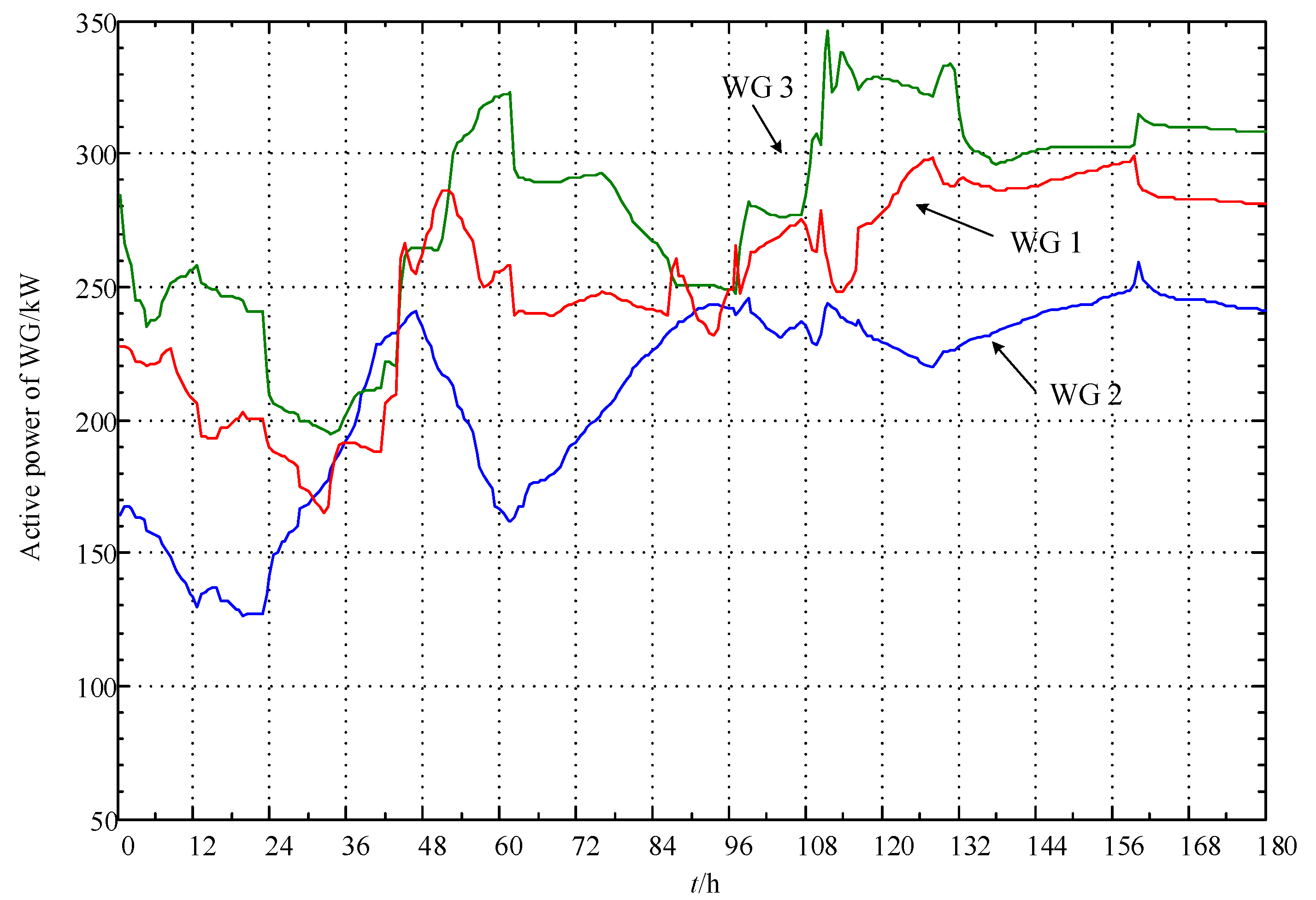
A simple scenario is firstly used to verify the effectiveness of the proposed DPF method, which is vitally important to the credible capacity index. In this scenario, all loads remain unchanged. Wind generations are calculated with commonly used active power output model based on meteorological wind speed data with public access, which can be downloaded on the website of the Earth System Research Laboratory (ESRL) that is affiliated to the National Oceanic and Atmospheric Administration (NOAA) of U.S. Department of Commerce [46]. The recorded meteorological in a typical week, which were collected from different monitoring stations without correlations, are used as input data to calculate active power output of WGs in this ADN case. It is shown in Figure 4.
As shown in Figure 4, wind generations in the hourly interval of (48, 56) are selected as input to be substituted into the proposed DPF model. The initial states of charge of all the energy storage devices are set to be 50%. Except for node voltage and branch line power flows, SOC curves of the four ESSs in 8 h can also be achieved, as shown in Figure 5.
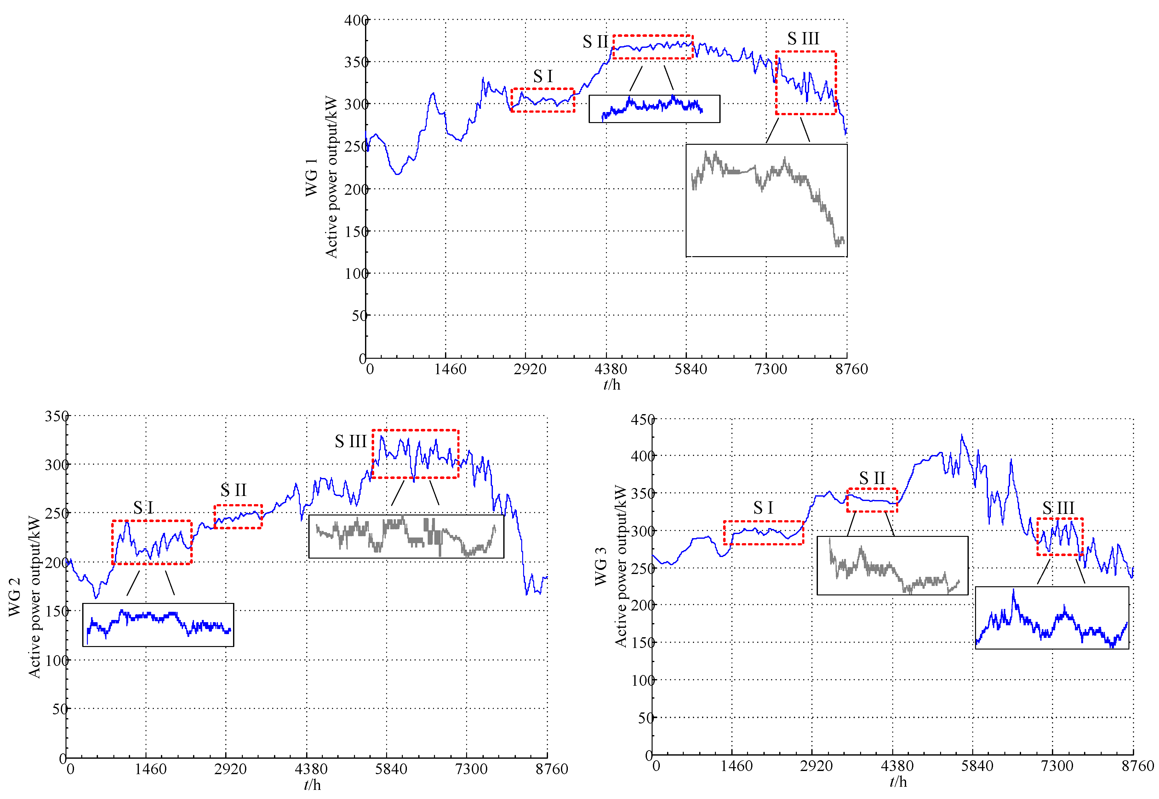
Further investigations are carried out. According to the fractal characteristic, wind generation’s background data chosen from different seasons of the year that apparently represent different scale free intervals and scenarios with different fractal dimensions are used. As shown in Figure 6, in this study case of the selected ADN network, active power output of the three intermittent wind generations is given according to basic meteorological data in reference [46].
As a topological invariant and a key feature of nonlinear dynamics system, fractal dimension can be calculated within a scale-free interval to quantitatively describe the irregularity [41]. If a complete graph is divided into many parts with the same size and shape, the definition of the most commonly used Hausdorff Dimension is given below [42].
Here, means the number of small parts, and r stands for the times that the original graph is larger than the smaller parts.
Due to differences on climate and other factors between each season, there must exist different scale-free intervals on the time continuous curves. Based on Equation (23) and the output curves of each WG power resources in Figure 6, some scale-free intervals on the curve are identified by calculating the fractal dimension. These scale free intervals represent different operation scenarios with various volatilities and irregularities of injected power of DERs. Related intervals are also marked in Figure 6. By utilizing the Hausdorff Dimension method, the value of fractal dimension of the studied curves as the input of DPF for credible capacity can be obtained, as shown in Table 2. The value differs from time and locations, but this reveals important indications.
On one the hand, the greater the value of fractal dimension is, the more irregular the geometry curve will be. A complete stochastic nonlinear system or a studying object deserves even larger fractal dimension of its key variables. However, the closer the value of the fractal dimension is to 1, the smoother the curve and more deterministic of its variation trend will be.
On the other hand, as a key feature of fractals that has been theoretically studied and demonstrated, self-similarity in the same scale-free interval as shown in the subplot of Figure 6 has been proven. It usually shares similar fractal dimension value in this interval, for example in one month. It means wind power generations of different time scale such as seconds or minutes can also represent power variations at hourly levels in the same scale-free interval. Therefore, each WG power resource’s basic generation data of minute time scale is extracted from each scenario on the curves, for further DPF calculation and credible capacity evaluation.
Specifically, for each scenario that corresponds to each scale-free interval, several groups of stochastic wind generation data are selected to form as many multiple operation sub-scenarios as possible. To examine the influence of operation scenario’s time duration on the value of credible capacity index, each group also contains data with different time periods varying from 5 min to 15 min. Namely, stochastic generation data fragments with various length of time periods are extracted from the same numbered scenarios of WG power resources to make up the overall operation scenarios.
Thus, based on the selected study case network and groups of stochastic wind generation data in three scenarios, the computation results of Equations (4) and (6), which are obtained by the proposed multi-scenario considered DPF method, and credible capacity value, which is calculated through Equation (3), are shown in Table 3 and Table 4.
Interval distribution and main statistical feature of credible capacity value are analyzed based on the groups of discrete data, as shown in Table 4. First, a scatter plot is shown in Figure 7. The values of credible capacity representing different scenarios of scale free intervals are marked in different colors. The size of bubble represents the time length of the scenario. It can be derived from the figure that the scatters with a larger size are generally closer to each other than those with a smaller size. This denotes that the values of credible capacity based on operation scenarios with longer time have higher accuracy. Besides, the value of credible capacity based on different operation scenarios with background data may differ from each other and fall into different categories.
Secondly, powered by the JMP statistical analyzing software (version 10.0.0, a production of the SAS Institute Inc., Cary, NC, USA), as shown in Figure 8, one-way analysis of variance (ANOVA) of credible capacity’s value from Table 4 is given. Significance level α is set to be 0.05. Solid Lines marked with green form the confidence interval of each group of data with a probability of 95%. The solid line connecting the average value of each group shows the trend line. Detailed critical indexes such as upper and lower limits of 95% confidence interval are given in Table 5, which are provided by ANOVA. As can be seen in the figure and table, correlations between each group of discrete data are not evident. Some of the standard deviations are intolerable. Thus, neither of these indexes can yet truly represent the true value of credible capacity with the minimum error.
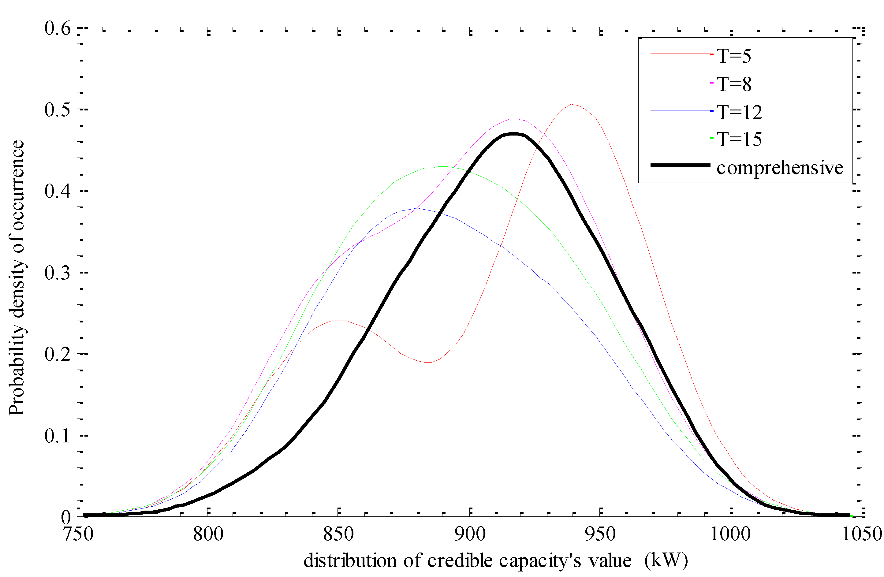
What is not known is the distribution law in one-dimensional interval of credible capacity value in Table 4, which is derived from DPF results of complete stochastic different scenarios. The kernel density estimation method is adopted as an approach of non-parametric estimation to calculate probability density function of credible capacity value’s distribution in the numerical interval of (750, 1050). The values of credible capacity are divided into four groups, calculated based on the scenarios with the same length of time period. Thus, the four probability density curves of the occurrence of credible capacity in this numerical interval are given in Figure 9, where dash lines marked in different colors. In addition, the whole sample being comprised of 72 individual values is also considered, of which the comprehensive probability density curve is plotted and marked in black solid line by MATLAB. In Figure 9, it can be seen that probability distribution of data in each group apparently differs from each other. Neither of these distributions belongs to standard normal distribution because of the prominent irregularities.
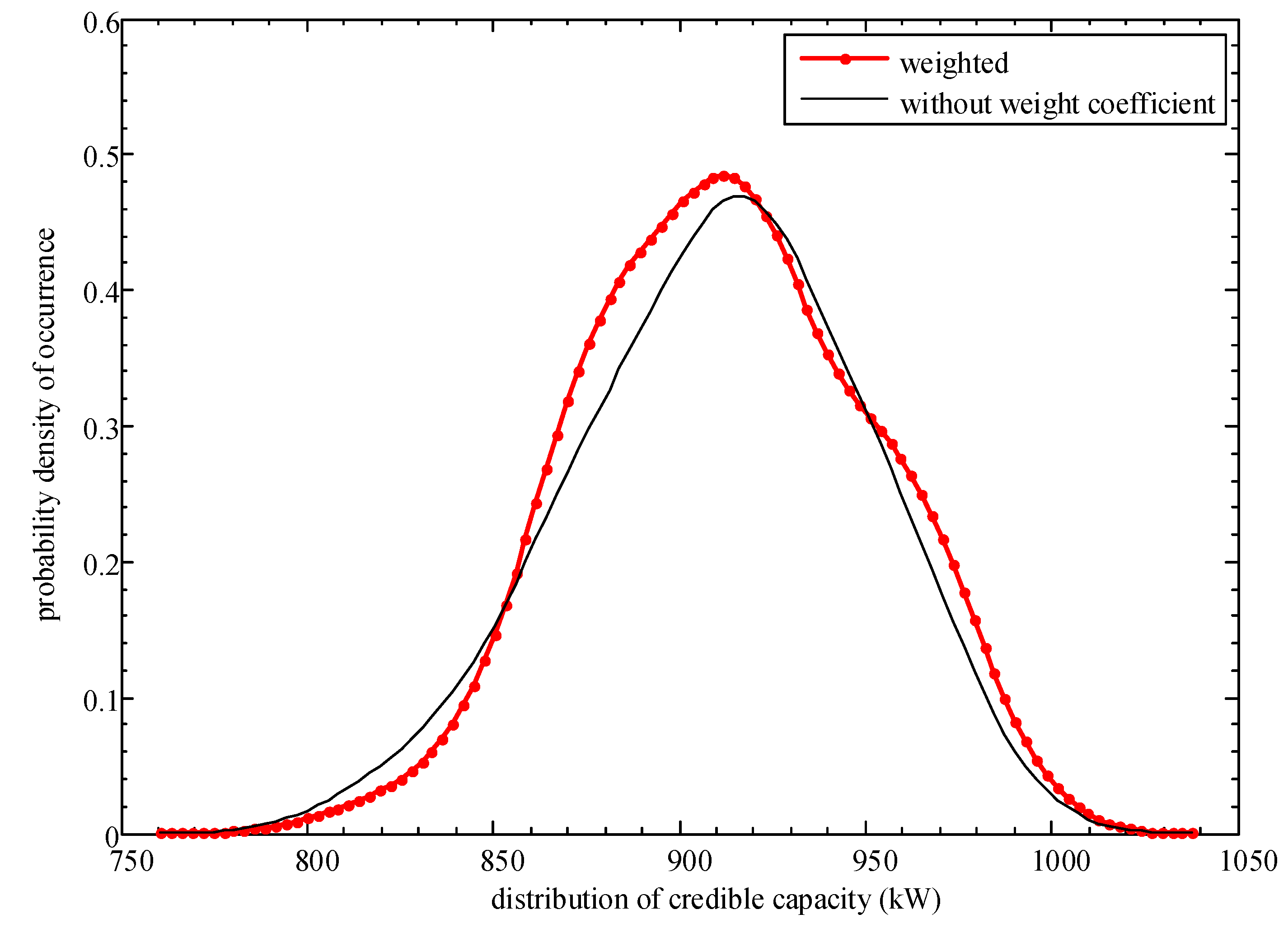
In the scatter plot of Figure 7, the value of credible capacity with larger size based on operation scenarios with longer time are closer to each other. This denotes higher accuracy. With this taken into account, weighted processed credible capacity values based on Table 4 are obtained to achieve the probability density distribution. As shown in Figure 10, a simple comparison in probability density of weighted credible capacity and value from Table 4 without weight coefficient is given. Credible capacity value in groups with longer time periods are assigned larger weights. This will be more reasonable and instructive. In Figure 10, it can be seen that the point with the maximum occurrence probability on weighted processed probability density curve is more likely to happen.
Therefore, the value with the maximum occurrence probability according to the weighted whole sample can be figured out by kernel density estimation method. Namely, 910.23 kW is decided as the final credible capacity value for this study case network. The interval estimation of credible capacity with different distribution probability levels based on the weighted whole sample’s probability density curve in Figure 10 according to Equation (1) is given in Table 6.
In this offline computing and analyzing process for calculating credible capacity, large computation is necessary. Considering this, statistical analysis or big data analytic method such as clustering can be used. The adoption of these more effective tools will be more appropriate to analyze numerous scenarios and larger samples, which can help lead to a more accurate result.
Obviously, the proposed method to evaluate credible capacity index of DERs cannot be directly compared with those classic probability methods in many aspects such as computation costs, complexity and efficiency, since they are completely different. As seen from the analysis above, it is certain that the deterministic credible capacity index surely reflects the operation situation and better improves the availability of grid analysis for optimization and control, when compared with that of probability methods in tackling with uncertainties and randomness.
Specifically, a simple case of grid extension planning applying the credible capacity of intermittent and controllable DERs is given, showing the improvements it brings.
Based on the study case ADN shown in Figure 3, assuming that an extension planning in the same area is needed to supply future power load demand 10 years later, a new substation should be built and the maximum load power of the year covering this area is estimated. Detailed specifications of the planning goal are given in Table 7. Up to three wind generators are planned to be integrated in the grid and the rated active power is 500 kW for each. The penetration rate of all integrated intermittent DGs are limited to be less than 25%.
Generally, to ensure safety and a complete consumption of intermittent DGs’ active power, not only the feeders have to meet transmission capacity constraints according to the rated power of DG, but also the design of substation outlets loops should reserve enough security margin. However, things will be different when it comes to the evaluated credible capacity value of current network. The coordination effect with ESS enables the DERs incorporating intermittent wind power to provide a relatively reliable and credible active power output, which can be quantitatively described by the credible capacity. Therefore, the planning budget with two more energy storage systems added applying credible capacity is illustrated as below.
With all DERs integrated, according to the final credible capacity evaluation results provided by this paper, the extended planning network in this area possesses a credible capacity value of 910 kW. As a result, if the DERs integrated operate normally, the year’s maximum load power that needs to be supplied by purchasing electricity from outside network declines to 5.39 MW. From an operation perspective, the year’s economic savings in electricity purchasing will be a deterministic value based on credible capacity and DPF method proposed in this work, rather than applying probability power flow methods. The year’s economic savings in electricity purchasing can be calculated through Equation (24), in which and represent the interval estimation result as shown in Table 6, according to the probability density curve of weighted processed credible capacity value. stands for the unified purchasing price regardless of time-of-use price. The electricity purchasing economic savings F in one year is still a conservative estimate value as the actual active power output of DERs may not always be 910 kW in real time operation.
Therefore, according to electric power balance result when applying credible capacity that is illustrated above, expenditure reduction in planning stage can be evaluated as follows. A widely used genetic approach is adopted as the planning method to come up with this extension planning case, as the same with other planning methods in the literature.
Firstly, two main distribution transformers configured in the substation to be built can be an option of rated capacity of 8 MVA for each. Because the year’s maximum load that needs to be supplied by purchasing electric power from transmission networks drops to 5.39 MW.
A more flexible grid structure is needed, which is designed with optimal shortest overall power supply path. It ought to help contribute to achieve minimal power losses and a balanced load distribution rate. These principles can be used to design a better planning case with intermittent power resources [47].
Secondly, the number of 10 kV feeder loops is not necessarily as many as that of planning case without applying credible capacity when the same type of feeder is adopted. Connection modes can also be different. Thus, for the planning case without credible capacity, 10 kV feeder lines with a total length of up to 36.18 km are needed. For the planning case with reference to credible capacity, the 10 kV feeder lines required just need to be 27.44 km.
Besides, the total length of branch lines for the two cases are 4.26 km and 1.49 km, respectively. The number of interconnection switches that need to be configured for the planning case without applying credible capacity is seven. However, for the planning case with reference to credible capacity, the number is five, according to the changes in connection mode.
In addition, each of the ESS configured in the planning network has a rated capacity of 3200 kWh. Therefore, according to the above mentioned items and by quantitatively estimating them one by one, the investigation expenditure and operation cost of two planning cases under similar reliability levels, namely without applying credible capacity and with reference to credible capacity, are listed in Table 8. Assume that the network load variations obey normal distribution.
In summary, economic savings in the above compared aspects are achieved owing to the reduction in operation cost and investigation expenditure for security margin, when applying credible capacity evaluation of DERs. The economic savings are calculated and estimated with the same planning method been used in other literature. In Table 8 it can be concluded that the planning case with reference to credible capacity has remarkable advantages in expenditure and cost reduction, when compared with planning case without applying credible capacity.
As illustrated above, credible capacity index of DERs can not only more accurately estimate electricity balance and make purchasing plan from transmission network, but also contribute greatly to grid extension planning in investigation expenditure reduction. Thus, the Distribution System Operators (DSO) will surely benefit from the advantageous application of credible capacity. This demonstrates that the deterministic value of credible capacity is more advantageous than probability method. Above all, the most important thing is that the credible capacity index reveals an intrinsic nature characteristic of ADN in complex and time-varying operation scenarios. A reliably evaluated credible capacity value of DERs denotes the reliability and power supply sufficiency reinforcement. Thus, in addition to planning benefits, the value can also be used in static security and analyze reliability more accurately when stochastic intermittent power resources are integrated. The capacity of controllable ESS is embedded in this index, which can also help improve the effect optimal control.
6. Conclusions
For grid analysis issues with uncertainties, generally, distributed generations are firstly modeled in terms of stochastic variables and then adopted in probability power flow method to obtain the system’s probability power flow distribution. In contrast, a credible capacity index incorporating intermittent distributed energy resources is defined. To solve this index, a novel dynamic power flow method considering multiple operation scenarios for active distribution network is proposed in this work. Specifically, the deterministic active power output of DERs is statistically calculated and evaluated based on the results of the proposed DPF method, according to multiple stochastic dynamic operation scenarios, which is better than predication or probability modeling.
The effectiveness of the proposed credible capacity index and multi-scenarios considered DPF method are demonstrated through selected study case network and pre-established scenarios, which is categorized by fractal dimension. The definition of credible capacity and its solution method are proven to be feasible. The value of credible capacity, which is derived from DPF results of those operation scenarios on minute level, can represent its true value to some extent. Several groups of credible capacity values are given and analyzed in a scatter plot. ANOVA results of these discrete data are given, and the value with maximum occurrence probability on the probability density distribution curve is decided as the final credible capacity result.
In addition, the credible capacity of DERs incorporating intermittent distributed energy resources is applied to a grid extension planning case. Through the comparison of electricity purchasing budget calculation and investigation expenditure estimation in Table 8, it demonstrates the significant cost reduction and technical advantages it can bring. This deterministic value also represents reliability and sufficiency reinforcement that the intermittent energy resources may have on the distribution grid for a secure power supply. It will help operation and control domain more accurately acquire the performance of intermittent DERs in active distribution network. Therefore, it is quite important for DSOs competing in electricity power market and can help them make better decisions. This may contribute to many issues such as static security and reliability analysis, real-time optimal control and so on, which can be further explored in future work.
Acknowledgments
The authors would like to appreciate the support of the National Natural Science Foundation of China (with issue number: 51677116).
Author Contributions
Chen Sun proposed and developed the systematic mathematical model, made the analysis based on data from study case and wrote the paper. Dong Liu proposed the concept of credible capacity of intermittent distributed generations, designed the whole study, and revised the paper. Yun Wang conceived and help performed the calculations and simulations. Yi You prepared the study case network, and provided important comments on the approach to the paper’s structure, modeling, and analysis.
Conflicts of Interest
The authors declare no conflict of interest.
Nomenclature
| Abbreviations | |
| DER | distributed energy sources |
| DG | distributed generation |
| ADN | active distribution network |
| ESS | energy storage system |
| EMA | exponential moving average |
| DPF | dynamic power flow |
| SOC | state of charge |
| ESRL | Earth System Research Laboratory |
| NOAA | National Oceanic and Atmospheric Administration |
| ANOVA | analysis of variance |
| DSO | distribution system operator |
| Sets | |
| the set of credible capacity’s value based on multiple dynamic scenarios. inf and sup are the upper and lower limit of the set | |
| simplified Jacobin matrix | |
| change quantity of each node’s phase angle compared to last balance state | |
| change quantity of each node’s voltage compared to last balance state | |
| a variable vector about node voltage in calculating the expanded Taylor series of system power loss | |
| Parameters | |
| the sum of active power output all DERs at specified time section t | |
| the sum of all loads at specified time section t | |
| , | active power injection of slack bus, and network active power loss at specified time section t. |
| credible capacity | |
| the sum of each load node’s average load active power within a specified time process | |
| average value of network active power loss | |
| average value of power injection of slack node | |
| β | the required probability of occurrence of each discrete credible capacity value in the interval |
| σ | smooth factor that varies from different time scales |
| the current output power of wind power | |
| PESS(t) | the real time active power output of ESS |
| P(t0) | the initial value of ESS |
| k | the slope of each line segment |
| Rc, Rd | charging and discharging rate |
| the energy capacity of ESS | |
| active power section in node power imbalance equations. stands for wind active power at node i. stand for load’s active power. is the output of ESS. U stands for node voltage amplitude. | |
| reactive power section in node power imbalance equations. stands for wind reactive power at node i. stand for load’s reactive power. U stands for node voltage amplitude. | |
| , , , , | stands for power factor. R for rotor resistance, Xm for exciter reactance, for the sum of stator reactance and rotor reactance of asynchronous generator. s for slip ratio |
| the network loss variation between two adjacent steady states | |
| the network active loss at the initial steady state | |
| the power loss variations’ average value | |
| the fractal dimension value based on Hausdorff Dimension method | |
| , r | the number of small parts, the times that the original graph is larger than the smaller parts |
| F, | electricity purchasing budget, unit price of purchasing electricity |
References
- Lopes, J.P.; Hatziargyriou, N.; Mutale, J.; Djapic, P.; Jenkins, N. Integrating distributed generation into electric power systems: A review of drivers, challenges and opportunities. Electr. Power Syst. Res. 2007, 9, 1189–1203. [Google Scholar] [CrossRef]
- Xue, Y.-S.; Lei, X.; Xue, F.; Yu, C.; Dong, Z.-Y.; Wen, F.-S.; Ju, P. A Review on Impacts of Wind Power Uncertainties on Power Systems. Proc. CSEE 2014, 29, 5029–5040. [Google Scholar]
- Banakar, H.; Luo, C.; Ooi, B.T. Impacts of wind power minute-to-minute variations on power system operation. IEEE Trans. Power Syst. 2008, 1, 150–160. [Google Scholar] [CrossRef]
- Foley, A.M.; Leahy, P.G.; Marvuglia, A.; McKeogh, E.J. Current methods and advances in forecasting of wind power generation. Renew. Energy 2012, 37, 1–8. [Google Scholar] [CrossRef] [Green Version]
- Xue, Y.-S.; Yu, C.; Zhao, J.-H.; Kang, L.; Liu, X.Q.; Wu, Q.W.; Yang, G.Y. A Review on Short term and Ultra-short term Wind Power Prediction. Autom. Electr. Power Syst. 2015, 6, 141–151. [Google Scholar]
- Abdelaziz, A.Y.; Hegazy, Y.G.; El-Khattam, W.; Othman, M.M. Optimal allocation of stochastically dependent renewable energy based distributed generators in unbalanced distribution networks. Electr. Power Syst. Res. 2015, 119, 34–44. [Google Scholar] [CrossRef]
- Deng, W.; Li, X.-R.; Li, P.-Q.; Li, J.X.; Sun, Q.; Chen, D.-L. Optimal Allocation of Intermittent Distributed Generation Considering Complementarity in Distributed Network. Trans. China Electrotech. Soc. 2013, 28, 216–225. [Google Scholar]
- Haesen, E.; Driesen, J.; Belmans, R. Robust planning methodology for integration of stochastic generators in distribution grids. IET Renew. Power Gener. 2007, 1, 25–32. [Google Scholar] [CrossRef]
- Xiang, Y.; Liu, J.-Y.; Li, F.-R. Optimal active distribution network planning: A review. Electr. Power Compon. Syst. 2016, 10, 1075–1094. [Google Scholar] [CrossRef]
- Shahirinia, A.H.; Hajizadeh, A.; Yu, D.C.; Feliachi, A. Control of a hybrid wind turbine/battery energy storage power generation system considering statistical wind characteristics. J. Renew. Sustain. Energy 2012, 4, 53–105. [Google Scholar] [CrossRef]
- Chen, F.; Liu, D.; Xiong, X.-F. Research on Stochastic Optimal Operation Strategy of Active Distribution Network Considering Intermittent Energy. Energies 2017, 10, 522. [Google Scholar] [CrossRef]
- Teleke, S.; Baran, M.E.; Bhattacharya, S.; Huang, A.Q. Optimal control of battery energy storage for wind farm dispatching. IEEE Trans. Energy Convers. 2010, 25, 787–794. [Google Scholar] [CrossRef]
- Wang, Y.; Liu, D.; Sun, C. A Cyber Physical Model Based on a Hybrid System for Flexible Load Control in an Active Distribution Network. Energies 2017, 10, 267. [Google Scholar] [CrossRef]
- Zhao, Y.; Zhou, W.; Yu, P.; Sun, H. Study on Regulation and Control of Active Wind Power Fluctuations. Proc. CSEE 2013, 13, 85–91. [Google Scholar]
- Yang, X.-Y.; Cao, C.; Ren, J.; Gao, F. Control Method of Smoothing PV Power Output with Battery Energy Storage System Based on Fuzzy Ensemble Empirical Mode Decomposition. High Volt. Eng. 2016, 7, 2127–2133. [Google Scholar]
- Wu, Z.-W.; Jiang, X.-P.; Ma, H.-M.; Ma, S.-L. Wavelet Packet-fuzzy Control of Hybrid Energy Storage Systems for PV Power Smoothing. Proc. CSEE 2014, 3, 317–324. [Google Scholar]
- Yu, W.; Liu, D.; Huang, Y. Operation Optimization Based on the Power Supply and Storage Capacity of an Active Distribution Network. Energies 2013, 6, 6423–6438. [Google Scholar] [CrossRef]
- Katinas, V.; Sankauskas, D.; Markevičius, A.; Perednis, E. Investigation of the wind energy characteristics and power generation in Lithuania. Renew. Energy 2014, 66, 299–304. [Google Scholar] [CrossRef]
- Boroumandjazi, G.; Rismanchi, B.; Saidur, R. Technical characteristic analysis of wind energy conversion systems for sustainable development. Energy Convers. Manag. 2013, 69, 87–94. [Google Scholar] [CrossRef]
- Li, J.-N.; Qiao, Y.; Lu, Z.-X.; Lu, J. An Evaluation Index System for Wind Power Statistical Characteristics in Multiple Spatial and Temporal Scales and Its Application. Proc. CSEE 2013, 13, 53–61. [Google Scholar]
- Yu, W.-P. Key Technical Index of Active Distribution Network and Its Application. Ph.D. Thesis, Shanghai Jiao Tong University, Shanghai, China, January 2014. [Google Scholar]
- Lin, W.-X.; Wen, J.-Y.; Ai, X.-M.; Cheng, S.-J.; Lee, W.-J. Probability Density Function of Wind Power Variations. Proc. CSEE 2012, 1, 38–46. [Google Scholar]
- Yang, M.; Qi, Y. Volatility of Wind Power Sequence and Its Influence on Prediction Error Based on Phase Space Reconstruction. Proc. CSEE 2015, 24, 6304–6314. [Google Scholar]
- Holttinen, H. Hourly wind power variations in the Nordic countries. Wind Energy 2005, 2, 173–195. [Google Scholar] [CrossRef]
- Gao, Y.-H.; Wang, C. Probabilistic load flow calculation of distribution system including wind farms based on total probability Equation. Proc. CSEE 2015, 2, 327–334. [Google Scholar]
- Cai, D.-F.; Shi, D.-Y.; Chen, J.-F. Probabilistic load flow calculation method based on polynomial normal transformation hypercube sampling. Proc. CSEE 2013, 13, 92–100. [Google Scholar]
- Zhu, X.-Y.; Liu, W.-X.; Zhang, J.-H. Probabilistic Load Flow Method Considering Large-scale Wind Power Integration. Proc. CSEE 2013, 7, 77–85. [Google Scholar]
- Ai, X.-M.; Wen, J.-Y.; Wu, T.; Sun, S.-M.; Li, G.-L. A Practical Algorithm Based on Point Estimate Method and Gram-Charlier Expansion for Probabilistic Load Flow Calculation of Power Systems Incorporating Wind Power. Proc. CSEE 2013, 16, 16–22. [Google Scholar]
- Gill, S.; Kockar, I.; Ault, G.W. Dynamic optimal power flow for active distribution networks. IEEE Trans. Power Syst. 2014, 1, 121–131. [Google Scholar] [CrossRef] [Green Version]
- Zakariazadeh, A.; Jadid, S.; Siano, P. Stochastic multi-objective operational planning of smart distribution systems considering demand response programs. Electr. Power Syst. Res. 2014, 111, 156–168. [Google Scholar] [CrossRef]
- Mokryani, G.; Hu, Y.-F.; Pillai, P. Active distribution networks planning with high penetration of wind power. Renew. Energy 2017, 104, 40–49. [Google Scholar] [CrossRef]
- Martins, V.F.; Borges, C.L. Active distribution network integrated planning incorporating distributed generation and load response uncertainties. IEEE Trans. Power Syst. 2011, 4, 2164–2172. [Google Scholar] [CrossRef]
- Muñoz-Delgado, G.; Contreras, J.; Arroyo, J.M. Multistage generation and network expansion planning in distribution systems considering uncertainty and reliability. IEEE Trans. Power Syst. 2016, 5, 3715–3728. [Google Scholar] [CrossRef]
- Jahromi, M.E.; Ehsan, M.; Meyabadi, A.F. A dynamic fuzzy interactive approach for DG expansion planning. Int. J. Electri. Power Energy Syst. 2012, 1, 1094–1105. [Google Scholar] [CrossRef]
- Voorspools, K.R.; D’haeseleer, W.D. An analytical Equation for the capacity credit of wind power. Renew. Energy 2006, 31, 45–54. [Google Scholar] [CrossRef]
- Zhang, N.; Kang, C.-Q.; Chen, Z.-P.; Zhou, Y.; Huang, J.; Xi, W. Wind Power Credible Capacity Evaluation Model Based on Sequence Operation. Proc. CSEE 2011, 25, 1–9. [Google Scholar]
- Wang, H.-C.; Lu, Z.-X.; Zhou, S.-X. Research on the capacity credit of wind energy resources. Proc. CSEE 2005, 10, 103–106. [Google Scholar]
- Vallée, F.; Lobry, J.; Deblecker, O. Impact of the wind geographical correlation level for reliability studies. IEEE Trans. Power Syst. 2007, 4, 2232–2239. [Google Scholar] [CrossRef]
- Vallée, F.; Lobry, J.; Deblecker, O. System reliability assessment method for wind power integration. IEEE Trans. Power Syst. 2008, 3, 1288–1297. [Google Scholar] [CrossRef]
- He, J.; Deng, C.-H.; Xu, Q.-S.; Huang, W.; Shu, Z. Assessment on Capacity Credit and Complementary Benefit of Power Generation System Integrated with Wind Farm, Energy Storage System and Photovoltaic System. Power Syst. Technol. 2013, 11, 3030–3036. [Google Scholar]
- Barnsley, M.F. Fractals Everywhere, 2nd ed.; Academic Press: New York, NY, USA, 2014; pp. 2–30. [Google Scholar]
- Hutchinson, J.E. Fractals and self-similarity, Department of Pure Mathematics, Faculty of Science, Australian National University. 1979. Available online: http://maths-people.anu.edu.au/~john/Assets/Research%20Papers/fractals_self-similarity.pdf (accessed on 27 July 2015).
- Jian-Kai, L.; Cattani, C.; Wan, Q.-S. Power load prediction based on fractal theory. Adv. Math. Phys. 2015. [Google Scholar] [CrossRef]
- Salvó, G.; Piacquadio, M.N. Multifractal analysis of electricity demand as a tool for spatial forecasting. Energy Sustain. Dev. 2017, 38, 67–76. [Google Scholar] [CrossRef]
- Wang, Y.; Niu, D.; Ji, L. Optimization of Short-Term Load Forecasting Based on Fractal Theory. In New Challenges for Intelligent Information and Database Systems; Springer: Berlin/Heidelberg, Germany, 2011; pp. 175–186. [Google Scholar]
- SURFRAD Data, Global Radiation Group, Earth System Research Laboratory. Available online: http://www.esrl.noaa.gov/gmd/grad/surfrad/index.html (accessed on 19 February 2014).
- Design and Operation of Power Systems with Large Amounts of Wind Power—Task 25. 2015 IEA Wind Anual Report. Available online: http://www.ieawind.org/annual_reports_PDF/2015/2015%20IEA%20Wind%20AR_small.pdf (accessed on 16 October 2016).
Figure 1.
Indicators reflecting variations of wind power.
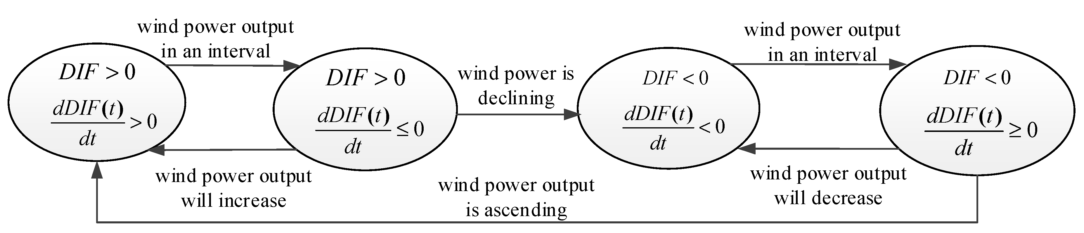
Figure 2.
The output power curve of ESS according to the variation of tracking indicator.
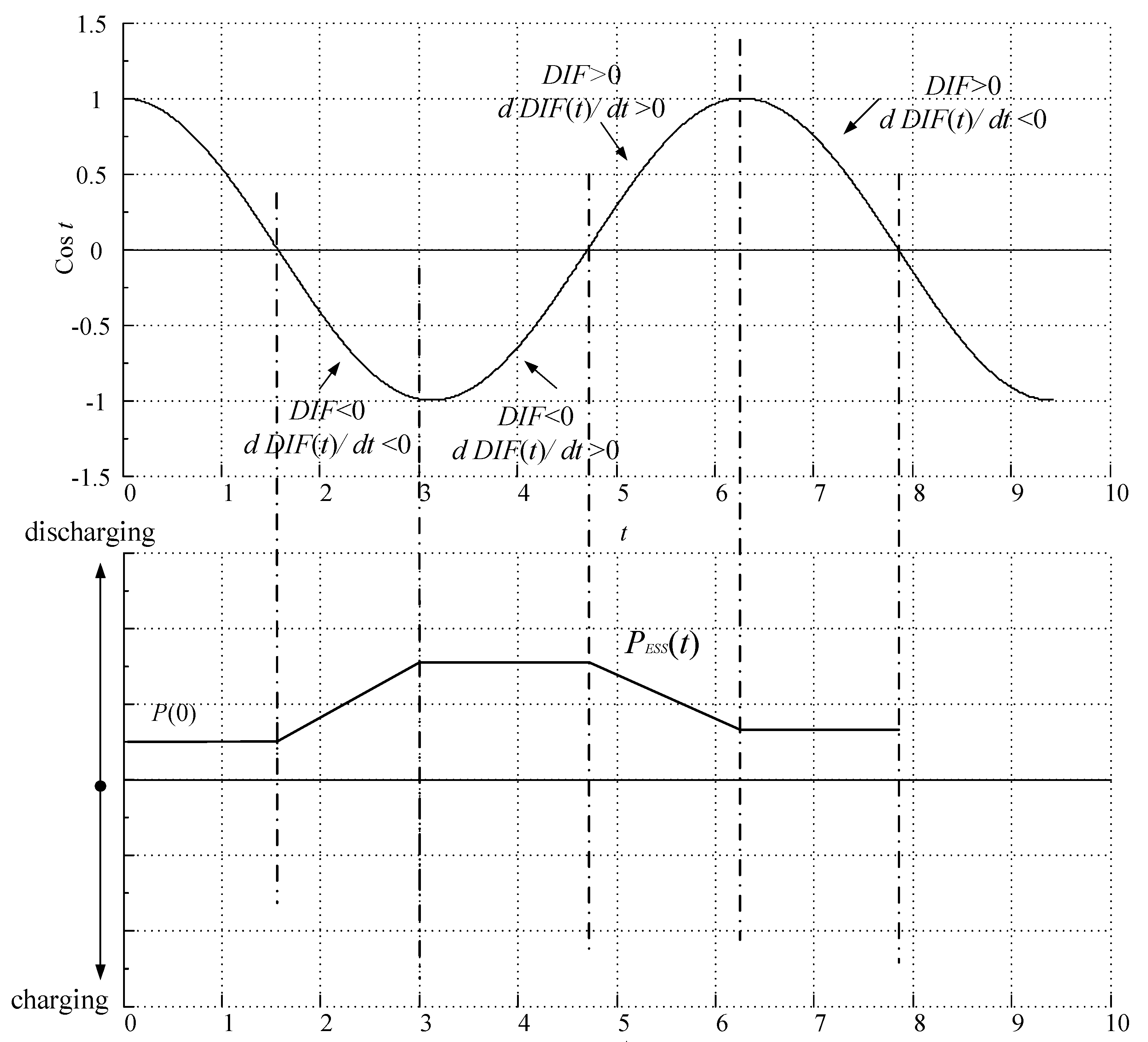
Figure 3.
Selected distribution network case with 32 nodes.
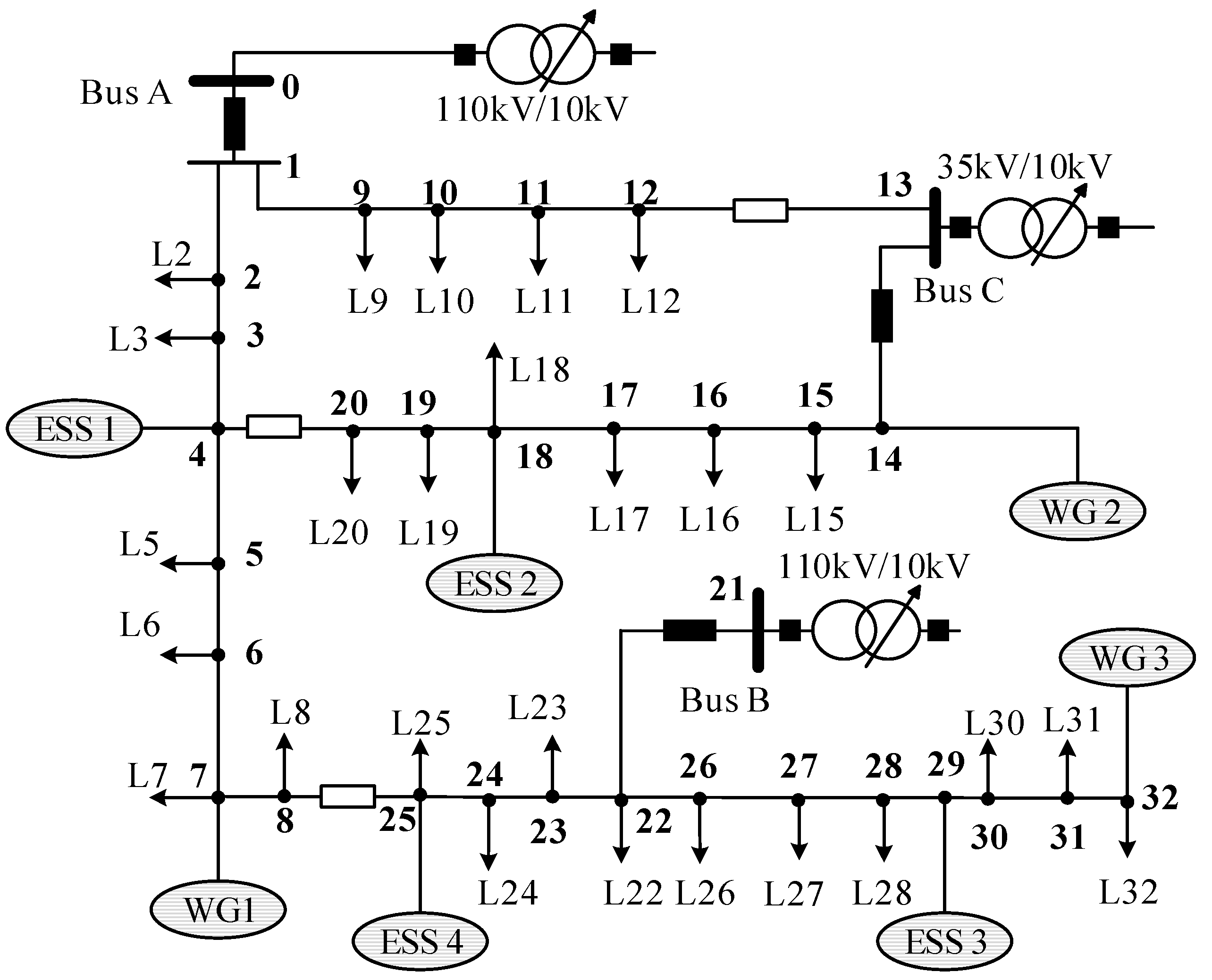
Figure 4.
Wind generations of the verifying scenario in a typical week according to public accessed meteorological data.
Figure 4.
Wind generations of the verifying scenario in a typical week according to public accessed meteorological data.

Figure 5.
SOC curves of the four ESSs within the specific time period.
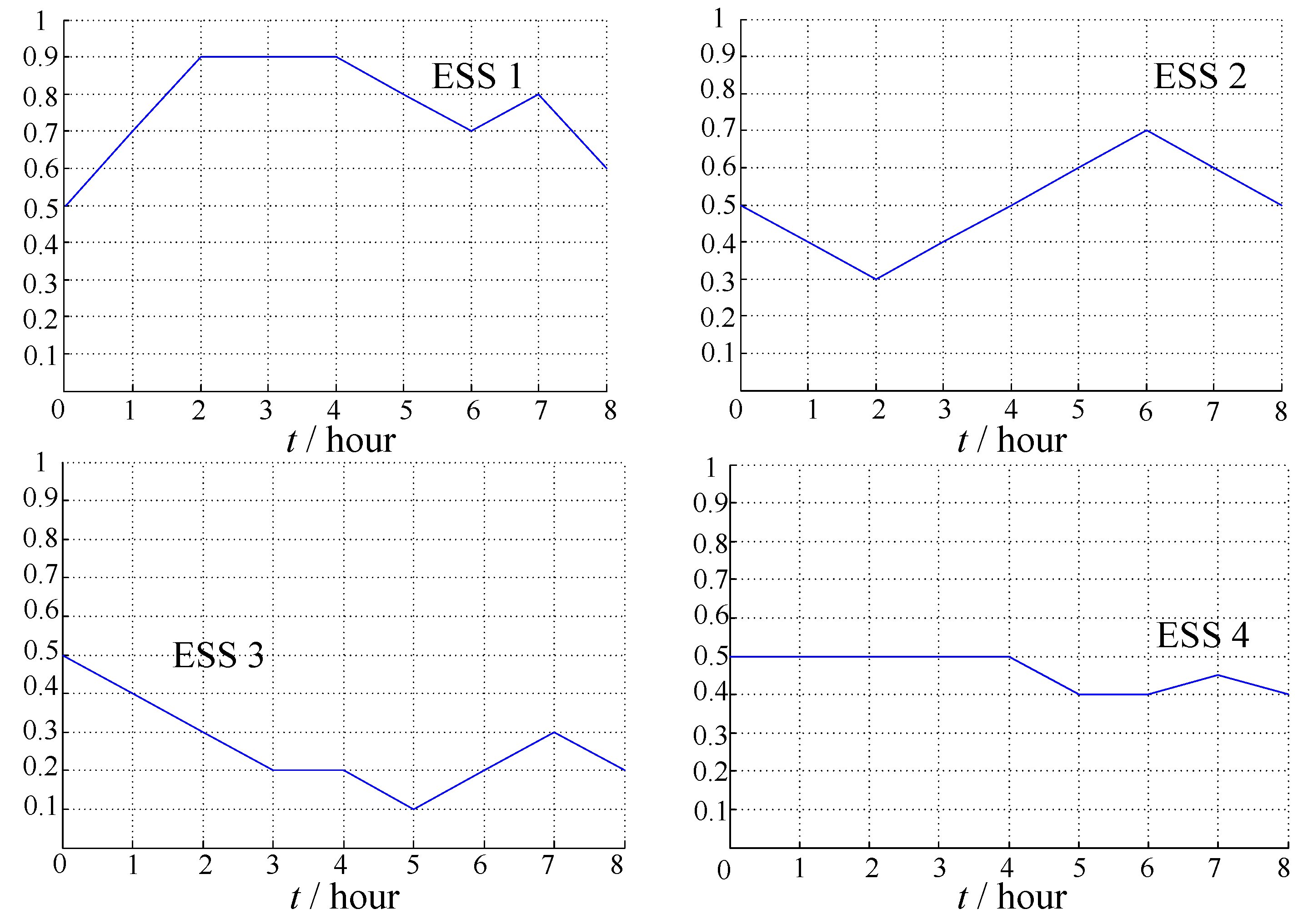
Figure 6.
Wind generation used in this case of a typical year.

Figure 7.
Scatter plot of the distribution of credible capacity’s value.
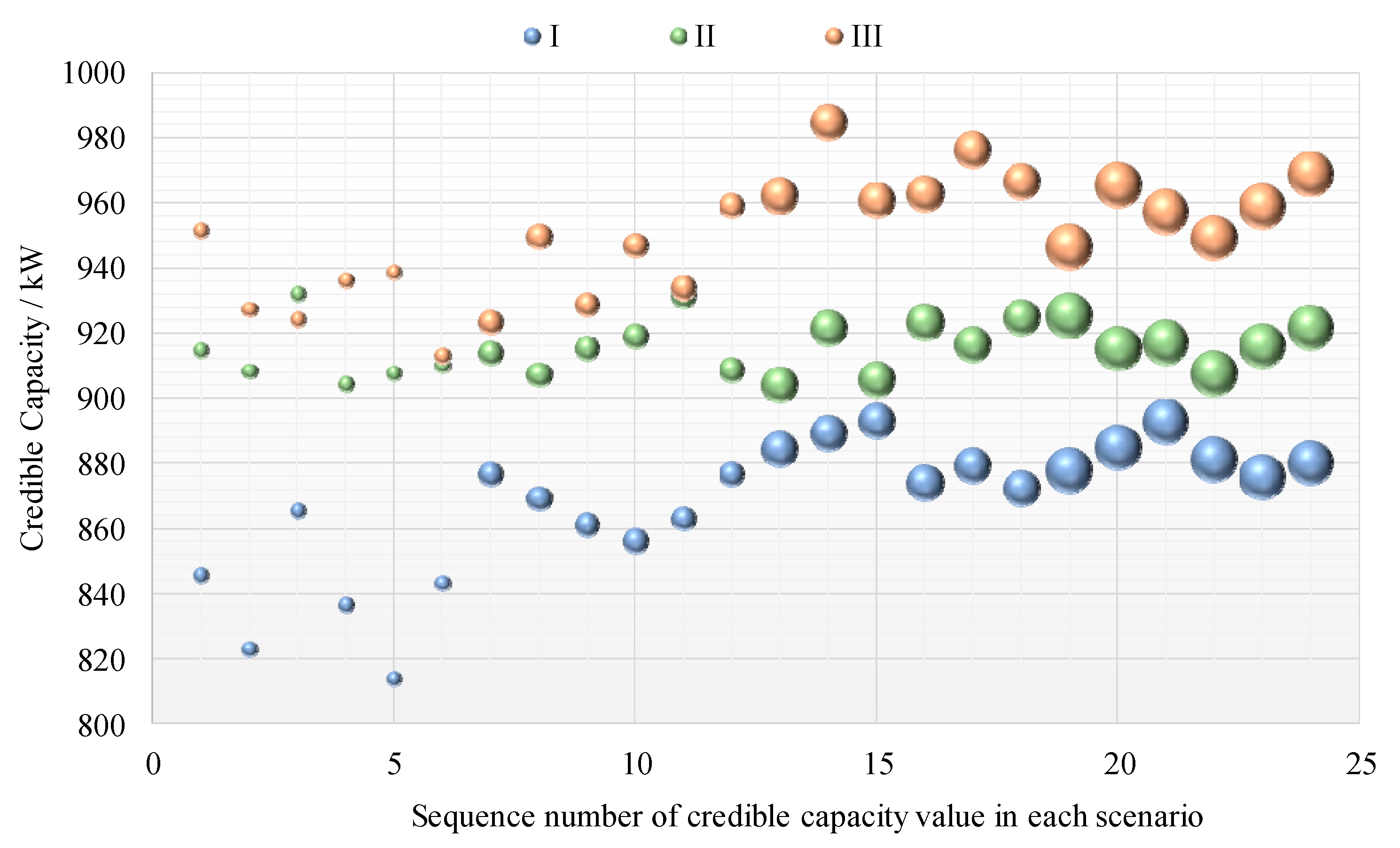
Figure 8.
One-way analysis of variance plot of credible capacity value from the three scenarios.
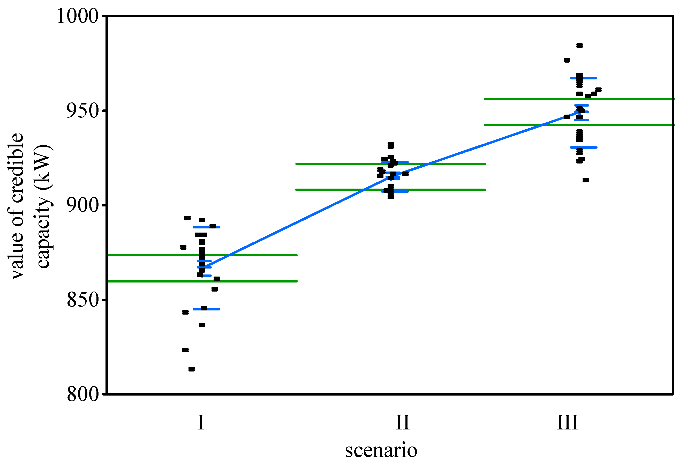
Figure 9.
Probability density distribution plot of credible capacity’s value.

Figure 10.
Probability density distribution plot of weighted credible capacity’s value.


Table 1.
Electrical specifications of the WGs/ESSs.
| Name | Rated Power | Rated Energy Capacity |
|---|---|---|
| ESS 1 | 300 kW | 2400 kWh |
| ESS 2 | 300 kW | 2400 kWh |
| ESS 3 | 400 kW | 3200 kWh |
| ESS 4 | 250 kW | 2000 kWh |
| WG 1 | 500 kW | - |
| WG 2 | 450 kW | - |
| WG 3 | 750 kW | - |
Table 2.
Fractal dimension results.
| Power Resources of the Output Curves | Scenarios | Fractal Dimensions | Whole Year | ||||
|---|---|---|---|---|---|---|---|
| WG 1 | S I | 1.154167 | 1.152820 | 1.154186 | 1.154868 | 1.154214 | 1.303953 |
| S II | 1.123417 | 1.125387 | 1.125542 | 1.125802 | 1.124593 | ||
| S III | 1.298209 | 1.296792 | 1.295391 | 1.295637 | 1.295516 | ||
| WG 2 | S I | 1.222479 | 1.222924 | 1.221129 | 1.221540 | 1.221302 | 1.347269 |
| S II | 1.162930 | 1.162800 | 1.161408 | 1.161202 | 1.161149 | ||
| S III | 1.323078 | 1.323061 | 1.324423 | 1.323038 | 1.324189 | ||
| WG 3 | S I | 1.178309 | 1.178519 | 1.178504 | 1.178701 | 1.178649 | 1.330167 |
| S II | 1.120026 | 1.119732 | 1.119202 | 1.120300 | 1.119666 | ||
| S III | 1.294800 | 1.293594 | 1.294235 | 1.294855 | 1.293523 | ||
Table 3.
Key variables of DPF results based on the three scenarios (scale-free intervals).
| Scenario | Variable | Group | 5 min | 8 min | 12 min | 15 min |
|---|---|---|---|---|---|---|
| I | (kW) | 1 | 5026.940 | 5202.471 | 5292.455 | 5292.428 |
| 2 | 5026.940 | 5202.471 | 5292.455 | 5292.428 | ||
| 3 | 5026.940 | 5202.471 | 5292.455 | 5292.428 | ||
| 4 | 5026.940 | 5202.471 | 5292.455 | 5292.428 | ||
| 5 | 5026.940 | 5202.471 | 5292.455 | 5292.428 | ||
| 6 | 5026.940 | 5202.471 | 5292.455 | 5292.428 | ||
| (kW) | 1 | 281.838 | 299.142 | 295.960 | 293.203 | |
| 2 | 260.716 | 285.263 | 301.647 | 298.055 | ||
| 3 | 288.657 | 282.131 | 307.609 | 303.686 | ||
| 4 | 265.145 | 283.408 | 304.206 | 297.4826 | ||
| 5 | 252.623 | 281.211 | 302.836 | 296.481 | ||
| 6 | 265.738 | 291.055 | 296.573 | 297.263 | ||
| II | (kW) | 1 | 5477.331 | 5495.920 | 5496.776 | 5503.839 |
| 2 | 5477.331 | 5495.920 | 5496.776 | 5503.839 | ||
| 3 | 5477.331 | 5495.920 | 5496.776 | 5503.839 | ||
| 4 | 5477.331 | 5495.920 | 5496.776 | 5503.839 | ||
| 5 | 5477.331 | 5495.920 | 5496.776 | 5503.839 | ||
| 6 | 5477.331 | 5495.920 | 5496.776 | 5503.839 | ||
| (kW) | 1 | 308.854 | 315.904 | 372.557 | 333.0869 | |
| 2 | 297.579 | 312.117 | 377.918 | 321.606 | ||
| 3 | 322.496 | 313.302 | 378.577 | 324.348 | ||
| 4 | 300.240 | 316.888 | 374.990 | 321.026 | ||
| 5 | 301.698 | 325.400 | 382.247 | 328.177 | ||
| 6 | 313.219 | 313.524 | 383.484 | 329.658 | ||
| III | (kW) | 1 | 5591.488 | 5642.422 | 5814.431 | 5747.085 |
| 2 | 5591.488 | 5642.422 | 5814.431 | 5747.085 | ||
| 3 | 5591.488 | 5642.422 | 5814.431 | 5747.085 | ||
| 4 | 5591.488 | 5642.422 | 5814.431 | 5747.085 | ||
| 5 | 5591.488 | 5642.422 | 5814.431 | 5747.085 | ||
| 6 | 5591.488 | 5642.422 | 5814.431 | 5747.085 | ||
| (kW) | 1 | 372.525 | 356.085 | 354.079 | 354.165 | |
| 2 | 359.658 | 358.253 | 378.429 | 369.294 | ||
| 3 | 359.001 | 357.448 | 352.509 | 359.182 | ||
| 4 | 362.041 | 357.787 | 366.413 | 360.638 | ||
| 5 | 359.814 | 357.945 | 371.167 | 362.133 | ||
| 6 | 355.529 | 369.120 | 367.306 | 365.979 |
Table 4.
Value of credible capacity based on DPF results of the three scenarios (scale-free intervals).
Table 4.
Value of credible capacity based on DPF results of the three scenarios (scale-free intervals).
| Scenario | Group | 5 min | 8 min | 12 min | 15 min |
|---|---|---|---|---|---|
| I | 1 | 845.575 kW | 876.671 kW | 884.405 kW | 877.898 kW |
| 2 | 822.886 kW | 869.094 kW | 889.424 kW | 884.874 kW | |
| 3 | 865.319 kW | 861.144 kW | 892.876 kW | 892.699 kW | |
| 4 | 836.381 kW | 856.065 kW | 873.961 kW | 881.045 kW | |
| 5 | 813.755 kW | 862.979 kW | 879.477 kW | 875.783 kW | |
| 6 | 843.024 kW | 876.519 kW | 872.313 kW | 880.131 kW | |
| II | 1 | 914.767 kW | 914.028 kW | 904.195 kW | 925.580 kW |
| 2 | 908.329 kW | 907.181 kW | 921.537 kW | 915.392 kW | |
| 3 | 932.128 kW | 915.399 kW | 905.911 kW | 917.286 kW | |
| 4 | 904.361 kW | 919.141 kW | 923.454 kW | 907.628 kW | |
| 5 | 907.521 kW | 931.453 kW | 916.735 kW | 916.168 kW | |
| 6 | 910.226 kW | 908.719 kW | 924.944 kW | 921.786 kW | |
| III | 1 | 951.555 kW | 923.492 kW | 962.382 kW | 946.527 kW |
| 2 | 927.373 kW | 949.779 kW | 984.892 kW | 965.720 kW | |
| 3 | 924.394 kW | 928.805 kW | 961.025 kW | 957.460 kW | |
| 4 | 936.132 kW | 947.104 kW | 962.924 kW | 949.364 kW | |
| 5 | 938.809 kW | 933.988 kW | 976.460 kW | 958.967 kW | |
| 6 | 913.225 kW | 959.255 kW | 966.749 kW | 969.047 kW |
Table 5.
Some critical indexes given by ANOVA.
| Group | Number | Average Value | Standard Deviation | Standard Error | 95% Lower Limit (kW) | 95% Upper Limit (kW) |
|---|---|---|---|---|---|---|
| I | 24 | 867.2623 | 21.22888 | 4.333327446 | 858.2982 | 876.2265 |
| II | 24 | 915.5778 | 8.198457 | 1.673502961 | 912.1159 | 919.0397 |
| III | 24 | 949.8095 | 18.34444 | 3.744543901 | 942.0633 | 957.5556 |
Table 6.
Interval estimation of credible capacity with different probability levels.
| β | inf (kW) | sup (kW) |
|---|---|---|
| 0.23058 | 899.000 | 923.000 |
| 0.46035 | 882.000 | 933.000 |
| 0.57888 | 872.000 | 943.000 |
| 0.69741 | 866.000 | 957.000 |
| 0.79515 | 860.000 | 969.000 |
| 0.83997 | 855.000 | 978.000 |
| 0.88236 | 849.000 | 985.000 |
| 0.92124 | 839.000 | 992.000 |
Table 7.
The goal and requirements of grid planning case.
| Planning Goal | Specifications |
|---|---|
| rated capacity of substation | 2 × 10 MVA |
| estimated year’s maximum load | 6.3 MW |
| estimated year’s minimum load | 4.1 MW |
| distributed generations to install | 3 WGs × 500 kW(rated power) |
| DG penetration rate limit | less than 25% |
Table 8.
Investigation expenditure and operation cost of the two planning cases.
| Categories | Planning Case without Credible Capacity | with Reference to Credible Capacity | Reduction Percentage |
|---|---|---|---|
| 110 kV substation | 160.00 | 100.00 | 37.5% |
| 10 kV feeders | 54.27 | 41.16 | 24.2% |
| branch lines | 4.26 | 1.49 | 65.0% |
| interconnection switches | 24.50 | 17.50 | 28.6% |
| energy storage systems | 400.00 | 400.00 | 0% |
| electricity purchasing/per year | 2368.70 | 2087.36 | 11.88% |
| sum | 3011.73 | 2647.51 | 12.09% |
(currency: RMB Chinese Yuan, unit: ten thousand).
© 2017 by the authors. Licensee MDPI, Basel, Switzerland. This article is an open access article distributed under the terms and conditions of the Creative Commons Attribution (CC BY) license (http://creativecommons.org/licenses/by/4.0/).
Share and Cite
MDPI and ACS Style
Sun, C.; Liu, D.; Wang, Y.; You, Y. Assessment of Credible Capacity for Intermittent Distributed Energy Resources in Active Distribution Network. Energies 2017, 10, 1104. https://doi.org/10.3390/en10081104
AMA Style
Sun C, Liu D, Wang Y, You Y. Assessment of Credible Capacity for Intermittent Distributed Energy Resources in Active Distribution Network. Energies. 2017; 10(8):1104. https://doi.org/10.3390/en10081104
Chicago/Turabian StyleSun, Chen, Dong Liu, Yun Wang, and Yi You. 2017. "Assessment of Credible Capacity for Intermittent Distributed Energy Resources in Active Distribution Network" Energies 10, no. 8: 1104. https://doi.org/10.3390/en10081104
Note that from the first issue of 2016, this journal uses article numbers instead of page numbers. See further details here.