The Optimal Generation Cost-Based Tariff Rates for Onshore Wind Energy in Malaysia
by
 , ,
, ,
Aliashim Albani
1,2,
Mohd Zamri Ibrahim
1,2,5,* ,
,
Che Mohd Imran Che Taib
1,3 and
Abd Aziz Azlina
1,4 1
Eastern Corridor Renewable Energy (ECRE) Research Group, Universiti Malaysia Terengganu, Kuala Nerus, Terengganu 21030, Malaysia
2
School of Ocean Engineering, Universiti Malaysia Terengganu, Kuala Nerus, Terengganu 21030, Malaysia
3
School of Informatics and Applied Mathematics, Universiti Malaysia Terengganu, Kuala Nerus, Terengganu 21030, Malaysia
4
School of Social and Economic Development, Universiti Malaysia Terengganu, Kuala Nerus, Terengganu 21030, Malaysia
5
TATI University College, Teluk Kalong, Kemaman, Terengganu 24100, Malaysia
*
Author to whom correspondence should be addressed.
Energies 2017, 10(8), 1114; https://doi.org/10.3390/en10081114
Submission received: 20 June 2017
/
Revised: 21 July 2017
/
Accepted: 25 July 2017
/
Published: 31 July 2017
(This article belongs to the Section L: Energy Sources)
Abstract
:The government of Malaysia has recently decided to explore the feasibility of wind energy to generate electricity in the country. Their ambition is to achieve a measureable target in the percentage contribution of electricity generated by renewable energy technology in the national electricity generation mix. As part of this initiative, a study of wind energy policy has been conducted by identifying the optimal feed-in tariff (FiT) rates to support the development of wind energy in the country. The aim of this paper is to calculate the optimal level of tariff that is suitable with local wind conditions. A closed-form equation for optimal feed-in tariff rate of wind energy with consideration of the availability of capital allowance has been developed. The focus is on small- and utility-scale wind turbine installations. As a result, by considering the availability of capital allowance, the optimal FiT rates for small-scale wind turbines in Malaysia are between 0.9245–1.1313 RM/kWh, while utility-scale rates are between 0.7396 and 0.9050 RM/kWh. The level of FiT is changed with the changing value of economic parameters. Kudat, in northern Borneo, has been identified as a prime site for wind energy development in the country; however, more work needs to be conducted, including the development of a regional wind map and measurement of wind data at more new potential sites.
1. Introduction
The demand for electricity in Malaysia is growing parallel with the Gross Domestic Product (GDP). This demand received a welcome boost from the roll-out of projects under the ongoing Five-Year Malaysia Plans and the Economic Transformation Programme (ETP). The generation of electricity has shown an increase of 3.7% in 2012 as compared to 3.1% in 2011 [1]. This growth has been driven by strong demands from commercial and domestic sectors. For the period until 2020, the average projected demand for electricity is expected to rise by 3.1%. Based on this forecast, the country is going to need even more energy as it strives to move towards a high-income economy. An estimated 10.8 GW of new generation capacity will be needed by 2020 given that 7.7 GW of the existing capacity is due for retirement. By 2020, the total installed capacity will see an increase of 16% over the total installed capacity in 2012. Of this new capacity, gas and coal will continue to feature strongly in Malaysia’s energy mix in the power sector, with coal probably taking up a bigger share on the basis of rising gas prices. However, due to the non-renewable nature of gas and coal, the resources are depleting at an alarming rate. In addition, the generation of energy from these non-renewable resources can emit greenhouse gases into the atmosphere, which is the principal cause of global warming. According to the recent publication by [2], the projected renewable energy (RE) share in the energy mix is expected to gradually increase up to 3–4% of total energy generated in years 2015 to 2025. This is very small compared to the non-renewable energy resources such as coal (48–66%), gas (23–46%) and hydroelectric (5%). In Malaysia, the mini-hydroelectric share is recognized as an RE resource in the Malaysia Renewable Energy Act 2011 [3], but not the large hydroelectric share. This is the reason the energy contribution of large hydroelectric is separated from the renewable energy in the national energy mix. Similar to Malaysia, the energy mix in other Southeast Asian countries such as the Philippines, Vietnam and Thailand is also largely comprised of the non-renewable energy resource such as coal and gas [4]. The projected contribution of RE in ASEAN countries from 2013 to 2040 is expected to decline from 26% to 21% due to the decreasing traditional use of biomass. The share of non-renewable energy in the energy mix is rising, from 74% in 2013 to a projected 78% in 2040 [4].
The government of Malaysia has thus realized the importance of renewable energy technology to generate electricity in the country. As early as 2007, the topic of renewable energy was suggested and debated in the parliament. In 2011, the Renewable Energy Act was passed by parliament, which set the framework for the remuneration of power producers for each kilowatt of electricity produced under the FiT scheme. Malaysia’s national target on the cumulative capacity of renewable energy is generated from four eligible RE resources: solar photovoltaics, mini-hydro, biomass and biogas. The targets for the year 2015, 2020, and 2030 are 985, 2080 and 4000 MW, respectively. However, the actual progress is dramatically different from the target thus far, where the cumulative capacity for the year 2015 was 320 MW, which is less than 50% of the original target of 985 MW [5]. According to a recent report by [6], the subsequent target also appears to be unachievable, as the projected capacity of RE-based energy in 2020 would be only 1464 MW assuming all the RE power plants were commissioned. Thus, the target for the year 2030 is sure to be completely off. Accordingly, one of the best solutions is to introduce a new renewable energy technology into the Malaysian RE mix to enhance electricity generation [5].
Wind energy is touted as the best candidate for newly eligible RE expansion in Malaysia. However, to initiate a wind energy project in Malaysia, a good policy needs to be established. The existing policies that implemented solar photovoltaic, mini-hydro, biogas, and biomass initiatives are not suitable for wind energy, as the nature of wind energy differs in several aspects, such as the site-dependent characteristics and the variation of specifications for wind turbine technology. The policy should cover a FiT system that corresponds to the wind conditions in Malaysia. The proper estimation of feed-in tariff rates is crucial, as the mishandling of tariff computations could lead to excessive or meager tariff payments that could either overburden the rate payer or cause the power producer to lose profit. Vietnam has experienced the negative effects of having tariff rates set lower than the actual generation costs, and it affected investors’ interest in the country’s wind energy industry. Although Vietnam has a high potential for wind energy compared to its neighboring countries like Thailand, the level of existing FiT rates will likely cause investors to lose profits as well as create a long pay-back period [6]. The FiT rate in Vietnam has been 0.0780 USD/kWh, compared to 0.1750 USD/kWh in Thailand [6].
The aim of this paper is to identify the baseline FiT rates for the wind-based energy producer in Malaysia. The tariff rates are based on the cost of generation for the recent practices in pricing the eligible renewable energy resources in Malaysia [7].
2. The Optimal Generation Cost-Based Tariff Model
The net present value (NPV) approach is selected for the cost-of-generation -based tariff determination. It is the best and easiest approach to define the profitability and levelize the overall costs [8]. The NPV of an investment is generally obtained by discounting all cash flows over the lifetime of the investment. The utilization of NPV in wind energy economic studies has been carried out in several studies [9,10,11]. The strong limitation of NPV as presented by [12] is the need for estimation of discounting rates. The uncertainty in the discounting rate estimation would affect the NPV cash flow. Therefore, the value of the discounting rate should be properly estimated. In spite of that, NPV would consider the time value of money and allows the computation of project value with different risk profiles [12].
In the current scenario, the tariff rates distinguish between the small-scale wind turbine (≤100 kW rated power) and utility-scale wind turbine (>100 kW rated power) [13], as the influences of economies of scale are considered. Nevertheless, one framework for both scales of wind turbines would be developed. Here, the difference between small and utility wind turbines is only in the initial capital cost per kW, thus the value of initial capital cost (CAPEX) in the equation can simply be adjusted without affecting the validity of the equation.
For the current study, the computation of FiT rates is comprised of four steps. First, CAPEX, annual operation and maintenance costs (OPEX), and the wind turbine (WT) component replacement costs were identified. The WT component replacement costs are costs associated with the replacement of any system component such as inverters, controllers or other electrical parts. The component should be replaced due to reduction of performance or failure to function. The replacement cost is assumed only once along the wind turbine lifetime.
Second, the debt calculation was considered in the investment cash flow. Third, the annual income generated by the electricity of wind turbines that transmitted to the grid were evaluated. Finally, the effects of capital allowance to the level of FiT were accounted.
The components of NPV that are utilized in the determination of FiT rates are divided into two: the cash inflow and outflow, as shown in Table 1. The derivation followed the simplified net present value [14] with small modification by considering the specific parameter assumption for Malaysia. The similar derivations were presented by [15,16].
The starting point to determine the optimal FiT rate in this case is to identify all costs involved in the cash outflow. Firstly, the initial capital cost (R) includes all upfront costs of the wind energy system: the cost of wind turbine modules, replacement, balance of system (BOS) and installation. Moreover, OPEX is defined annually where the annual percentage of OPEX is multiplied with the CAPEX. The last cost involved in the cash outflow is the WT components replacement cost, where the estimated percentage of cost of WT components is multiplied with the CAPEX. Certain WT components are assumed to have to be replaced after 10 years, half of a wind turbine’s projected lifetime. Therefore, the WT components replacement cost in 10 years would be discounted to its present value.
Following these steps, the annual cash outflows from the debt repayment and the debt interest were established. The value of the debt is given by the share of debt in the investment (1 − θ) multiplied with the initial capital cost (R). The debt maturity, in years, is given by M. Hence, assuming an equal amount is repaid every year, the annual repayment is: R(1 − θ)(1/M). For the debt interest, the debt share that is still outstanding in that year is multiplied with the interest rate (r) and corporate tax rate (τ).
In Malaysia, the tax savings can be added to the cash inflow by considering the capital allowance (CA), which is a benefit for corporate feed-in approval holders (FiAH) as mentioned in schedule 3 of the Income Tax Act 1967 [17]. Under CA, the renewable energy system is categorized as plant and machinery and it is qualified for depreciation over the period of six years. The CA in Malaysia comprises the following types of provisions: (i) initial allowance (IA—for the first year allowance); (ii) annual allowance (AA—for subsequent years until the full amount is utilized); and (iii) balancing allowance. The CA percentage of initial allowance is fixed at 20%, the annual allowance is 14% for five years, and the balancing allowance is 10%. The annual tax saving is computed by the CAPEX multiplied with CA percentage and the corporate tax rate.
In addition, the annual income coming from the tariff remuneration for selling electricity to the grid, must be considered. It is computed by the multiplication of FiT rates, wind turbine rated power, capacity factor, and hours in a year (8760 hours/year): F(PR)(CF)(H). Here, the output of a wind turbine is assumed to degrade annually as mentioned by [18], therefore the degradation rates, γ would be included in the income equation. In addition, it is desirable for a FiT policy framework to include a degression rate, . The inclusion of degression rate in the closed-form equation of FiT rate determination would derive the optimal FiT rate. Both wind turbine degradation and FiT rate degression would occur starting in the second year of operation.
The cash inflow components include the income from energy produced and the capital allowance. Consequently, the components of cash inflow can be presented as the following:
The components of cash outflow include the share equity of total cost, discounted operation and maintenance cost, debt repayment, and the WT component replacement cost. The components of cash outflow can be presented as the following:
Therefore, the NPV for the project over Renewable Energy Power Purchase Agreement (REPPA) periods can be calculated as the following:
where, N is the REPPA periods; PR is the rated power of wind turbine; is the FiT rate; CF is the capacity factors; is the hourly loads per year; τ is the corporate tax; is the discounting rate; is the cost degression; γ is the degradation of AEP; R is the CAPEX; θ is the percentage for the share of equity; (1 − θ) is the percentage for the share of debt; is the loan maturity periods; r is the interest rate; φINV is the percentage of cost of WT component replacements that have to be replaced; nINV is the specific year component replacement cost; and φOM is the percentage of annual O & M.
If the NPV for a project is positive, this means that the investment is economically viable. Therefore, if we set the NPV to zero and solve F, we can obtain the baseline FiT, the breakeven point for the project in which they get the rate of return in the project.
3. Parameter Assumptions for Malaysia
The FiT rate calculations for Malaysia are based on the following given information: (i) previous academic research and case study reports on the economics of wind energy; (ii) the national law documentations; and (iii) a series of communications conducted with industry experts at the Renewable Energy Workshop in Year 2015 in Selangor, Malaysia, and the Asia-Pacific Economic Cooperation (APEC) Seminar for Best Practices on Wind Energy in Year 2016 in Hanoi, Vietnam.
The uncertainty of estimated parameter values was minimized by careful justification and computation. In the following Section 4.1, the sensitivity analyses were carried out to define the effect of different uncertain input parameters to the value of optimal tariff rates.
3.1. The Investment Cost
The investment cost is the total cost of a wind project, which includes the wind turbine system, installation, and maintenance cost. The turbine has the highest percentage of initial capital cost for the onshore wind project, which is around 71% of the total cost [19]. The remaining cost is used for construction-related costs, which are only 29% of the total cost as there is no additional cost for the foundation of wind turbine tower [19]. Most of the onshore wind energy projects have been located near grid transmission lines, and hence have less costs for new transmission line installation.
In this regard, the Renewable Energy Policy Network for the 21st Century (REN21) released their 2016 annual report about the investment cost for Asian countries, and the reported costs are between 956 and 2784 USD/kW with the average of 1280 USD/kW [20]. The investment cost depends on the maturity of technology and market in the country. In a case involving a country that intended to develop its first wind energy project, the maximum amount of initial investment cost should be presumed, to reduce faulty assumption. The best approach in assuming the cost of wind turbines is by observing the success of the neighboring countries. Thailand and Vietnam are well-known for their wind energy development in Southeast Asia. The investment cost of wind energy projects for both countries, and the amount of initial investment cost, has ranged from 1000 to 3500 USD/kW [21,22,23,24]. Thus, the estimated initial capital cost of a wind turbine in Malaysia should be in the mentioned range.
The cost of a wind turbine is also influenced by economies of scale, where the costs are reduced due to technology learning. Over time, the increased turbine sizes have been followed by economies of scale in project size and manufacturing [25]. Specifically, the innovations in design, materials, processes, and logistics have helped to drive down the system and components’ costs while facilitating turbine up-scaling. In other words, the cost in RM/kW for a small-scale wind turbine (below than or equal to 100 kW) is always higher compared to the utility-scale wind turbine (more than 100 kW capacity). Usually, the price per kilowatt for the utility-scale is around 25% cheaper than the small-scale wind turbine [13,26].
Malaysia has not yet developed any commercial wind park; therefore, there are no official data of investment costs reported in any form of publication. One of the criteria in cost assumption is to use the cost data from the invoices by the manufacturers as a reference. Therefore, the assumed CAPEX of a small-scale wind turbine for Malaysia is 12,500 RM/kW, while the utility-size wind turbine is 10,000 RM/kW. The estimated CAPEX is confirmed with the reported data of CAPEX in Asia [20], and the neighboring countries. The estimated CAPEX is also in line with the estimation by [27] after summing the turbine-generator price, freight cost, balance of plant and installation costs and annual overhead costs except maintenance cost. The annual operational and maintenance cost for OPEX is estimated as 2% per year.
3.2. Degression Rate
The degression is related to the annual reduction of wind turbine capital cost. Degression should be included in the FiT rate determination model as the rates should be timely adjusted in accordance with the technology advancements. Degression has been adopted by many countries that have implemented the FiT policy, including Malaysia [6].
In order to estimate degression rates, the history and recent trend of declining costs should be taken into consideration. The initial capital cost of wind energy projects would usually decline annually. The average annual degression in the United Kingdom is lower than the previous years, where the values are between 0.5% and 1.5% [28]. The report by [28] is supported by a report by [29] on the projection that by the year 2030, the cost reductions will be around 1% per year. However, Germany has an early reduction that is below 1% and the degression percentage of onshore wind energy is 0.4%. However, the facility for renewable energy is not matured in Malaysia; therefore, in this regard, 1% is a safer assumption for wind energy in the country
3.3. Baseline Capacity Factor
The other main criteria that has to be taken into consideration in the FiT rate determination is the baseline capacity factor (CF). The baseline capacity factor is the minimum capacity factor that should be produced by a wind turbine or a wind park to be eligible for the FiT program. The capacity factor is directly affected by the efficiency of the wind turbine and the quality of wind speed at the site. It was discovered that not all sites are feasible for wind energy production in Malaysia, as it is largely situated in a low-wind-speed region. Thus, a minimum capacity factor should be stated to ensure the approval for the FiT program. Any project with the capacity factor below the CF baseline will be rejected and deemed not feasible for the FiT program. If a low CF project is accepted, there will be losses, as the given FiT rates will not allow the cash flow to achieve or exceed the breakeven threshold during the REPPA period.
Many countries have implemented the minimum capacity factor, including Iran with the minimum CF set at 20% [30,31], Pakistan at 31% [32], and Russia at 27% [33]. In Maharashtra, India, they adopted the minimum wind power density, in which the tariff is only eligible to projects on a site with at least 200 W/m2 [34].
In order to determine the baseline capacity factor for the wind energy in Malaysia, the researchers and FiAHs agreed that the best minimum capacity factor is 20%, as it would give a good return to the investment on wind energy. In other areas’ experiences, for example, an effective capacity factor in Massachusetts as discovered by [35] is between 20% and 30%. Spellman and Stoudt (2013) also confirmed that the capacity factor for the success of wind park operations is in the range from 20% to 35% [36]. The capacity factor of wind turbines can be compared with factors that are more than 50% for fossil-fuel power plants and over 60% for new gas turbines.
3.4. The Parameters of Debt Repayment
It is common practice for the investor to apply the loan from a finance agency to cover the higher initial capital cost of a wind energy project. Project developers would obtain the capital for the initial cost through the combination of debt (a loan) and equity investment (ownership). Usually, the bank will not give the full 100% loan, and may only loan 80%, as similar for the average share of equity for countries such as Denmark, Germany, The Netherlands, Spain, Sweden, Switzerland, and United States [37]. In Malaysia, the value of debt interest could be up to 18% without collateral or 12% with collateral as stated in the Moneylenders Act 1951 [38]. However, the minister has the power to decide the acceptable bank interest rate where the interest is less than 6%. For renewable energy in Malaysia, the value of risk-free rate or debt interest is 5% [39]. The debt is assumed to be discrete from the other loans that a power producer may have.
3.5. The Discount Rate
The discount rate is used in a discounted cash flow analysis to compute the net present value. In order to compute the levelized cost of energy for wind energy, REN21 gave a 7.5% discount rate for Organization for Economic Cooperation and Development (OECD) countries, and China and the rest of the world are only given 10% [20]. The OECD is a unique forum where the governments of 35 countries work together to promote economic growth, prosperity, and sustainable development [40]. Malaysia is a non-OECD country; thus, 10% is the discount rate for the Levelized cost of energy (LCOE) calculation. However, the value of 10% does not consider the effect of debt. This study has estimated the discount rate using the weighted average cost of capital (WACC) method. The WACC is a blend of the cost of equity and the after-tax cost of debt. The WACC equation is as follows:
where, θ is the percentage for the share of equity, (1 − θ) is the percentage for the share of debt, ce is the cost of equity, cd is the cost of debt, and τ is the corporate tax.
The cost of equity, ce is the minimum rate that a company desires to earn when investing in any project. It is also referred to as the company’s required rate of return or target rate. The average for wind energy is around 10% to 12%. The value of 10% is used in the estimated unleveraged discounting rates that are utilized for the LCOE calculation in the recent RE report [20].
The pre-tax cost of debt, cd, is the sum of the risk-free rate, r, and the default spread, rs; where, cd = r + rs. The value of risk-free rate is 5% [39], while the default spread for Malaysia is 1.35% [41]. Thus, the value of pre-tax cost of debt is 6.35%. The WACC for 20% of share of equity is 5.81%.
Therefore, the final assumptions for the economic parameter values that are used to calculate the baseline FiT rates for wind energy in Malaysia are presented in Table 2.
4. Results and Discussion
The derived model can be applied to determine the optimal tariff for wind energy at other country locations. However, the specific local law (such as the type of depreciation for tax savings) should be considered during the utilization of the model. The derived tax saving equation can be eliminated from the closed-form equation or replaced with the particular country’s type of tax saving equation. The straight-line depreciation method has been widely used by many studies including [16], and can be included in the model. For the straight-line depreciation, the annual value of the depreciation is computed by CAPEX divided by the REPPA period and, multiplied by the corporate tax rate.
4.1. Sensitivity Analysis
The baseline FiT rates are actually the levelized cost of energy, which represents the sum of all the costs over the lifetime for a given wind project. Then, it is discounted to the present time and levelized based on the annual energy production. Determining the baseline FiT rates requires the evaluation of several components, including cost streams that vary over the lifetime of the project. The generated baseline FiT rate is very sensitive to the value of the following parameters: (i) baseline capacity factor, (ii) the discounting rates, (iii) initial investment cost, (iv) the share of equity and debt, and (v) the capital allowances.
4.1.1. The Impact of Investment Cost on the Baseline FiT Rate
One of the most important factors in the FiT rates closed-form equation is the initial capital cost as it is the main contributor in the cash outflow. By referring to the base case (12,500 RM/kWh for small-scale wind turbine and 10,000 RM/kWh for utility-scale wind turbine), the sensitivity analysis was up to ±30%. The ±30% is utilized as it would generate the initial investment cost in meeting the range of investment costs reported for wind energy projects globally, in Asia, and in Malaysia’s neighboring countries. Table 3 shows that the baseline FiT increases in accordance with the increment of investment cost. Thus, the baseline FiT is expected to decrease annually due to the annual degression of wind turbine cost.
4.1.2. The Impact of Debt on the FiT Rates
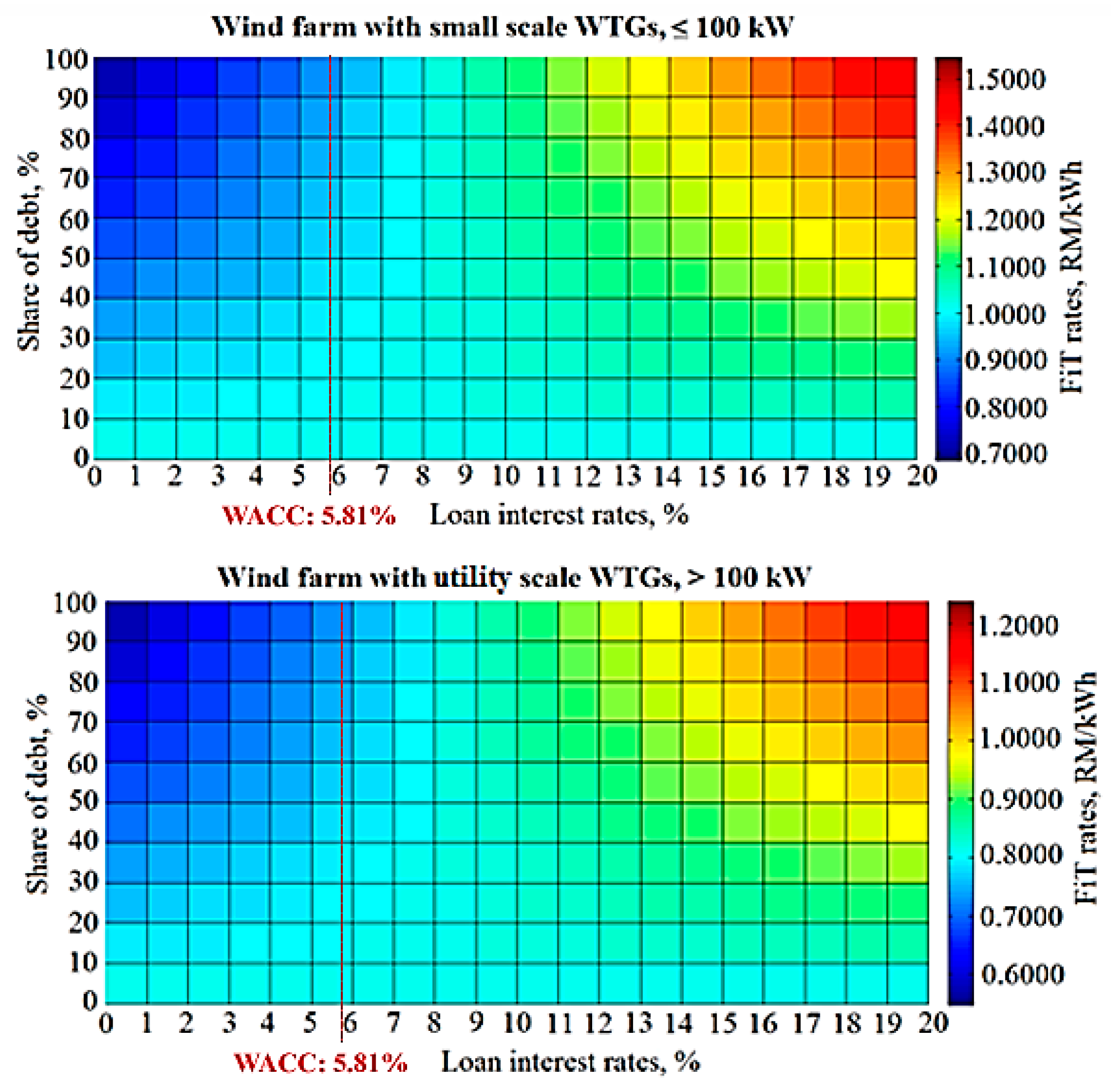
The relative values of the debt interest rate and nominal discounting rate will affect the relationship between debt fraction and FiT rates. Figure 1 gives an example for a standard loan in this context; when the loan interest rate is lower than the nominal discounting rate (5.81%), the FiT rates would decrease with the increment of debt fraction. This happens because of the amount of debts that were discounted throughout the period of years until loan maturity. The discounted amount of debt would decrease and be summed with the non-discounted amount of equity. Then, the total amount would be less than the original amount of initial capital cost with 100% equity.
In other conditions where the loan interest rate is greater than the nominal discounting rate, the FiT rates would increase with the increment of debt fraction. This is the normal condition when the power producer has to take a loan, and the debt interest rate would increase the value of cash outflow that thus increases the FiT rates. The increment of the discounting rates would be lowering the present value of cash outflow, while the increment of loan interest rates would increase the present value of the cash outflow. The existence of both variables in the loan repayment equation is the reason for the up and down trends (see Figure 1). The government should provide low-interest loan programs that can significantly reduce the cost of project supply to support the wind energy project in the country. This action would increase the relative competitiveness of wind energy in relation to the other energy generation technologies.
4.1.3. The Impact of Capacity Factor and Discounting Rates
The crucial risk that would affect any wind energy project is its eligibility in terms of energy production and economic aspect [43]. The nature of wind energy itself is intermittent, and the fact that Malaysia is located in a low-wind-speed region might worry the potential FiAH on the risk. The proper design of policy should be able to reduce the eligibility risk. Eligibility risk refers to the risk that a particular project may be deemed as ineligible for the FiT scheme after the occurrence of significant cash outlays during the project’s development [44]. In order to reduce or eliminate this risk, the government should give some time for conditional determination of eligibility before beginning the wind park construction and operation. In addition, clear policy guidelines and rules can reduce the confusion on which types of projects are eligible. Therefore, the floor capacity factor should be introduced and implemented, where 20% is the best minimum capacity factor for the renewable energy project. Figure 2 shows the sensitivity analysis for the impact of CF with the level of FiT. The FiT rates were determined based on the baseline capacity factor; thus, CF has a big impact to the level of FiT. The FiT would increase with the decreasing value of CF. So, the best baseline CF should be carefully chosen. The selection of low baseline CF will allow more project proposals to be accepted for the FiT scheme. However, it might burden the rate payer by remunerating high FiT rates to FiAH. If the baseline CF is set too high, fewer project proposals would be accepted as not many places have the potential for the development of wind energy projects. Besides that, the high baseline CF might cause the FiT to be lower and less attractive to the investors.
4.2. Economic Analysis
4.2.1. Case Study Site and Energy Analysis
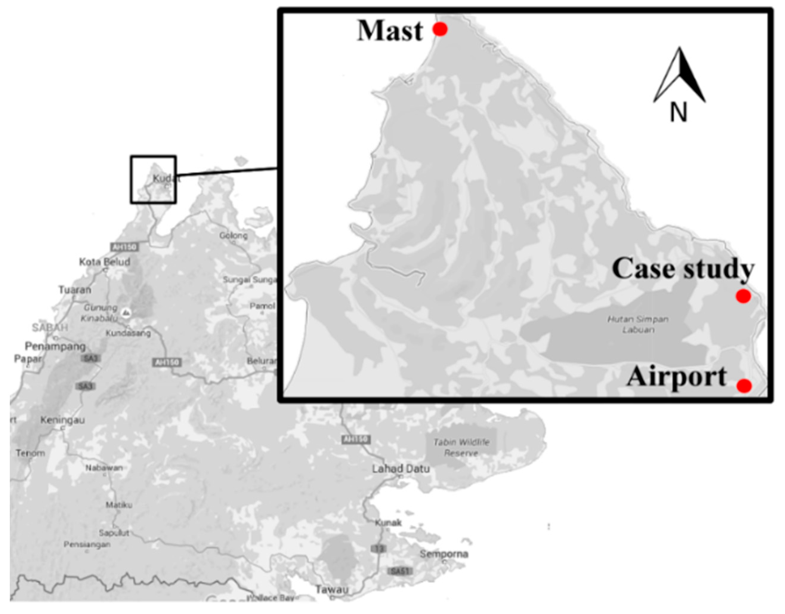
A site in Kudat, namely Bak-bak, was selected as the case study site (see Figure 3). The result of wind resource and energy production analysis were extracted from a recent report by [45], which also conducted a similar study on wind energy at the same site. The center coordinates are N 6°56’46.9’’, E 116°49’43.5’’. Kudat is a town in Sabah that is situated in the East of Malaysia. From the West, Kudat faces the South China Sea and it faces the Sulu Sea at the east direction. As reported by numerous scholars, Kudat is a well-known region that has promising wind energy potential in Malaysia [46,47,48,49].
The wind speed data were collected from the measurement mast developed by Universiti Malaysia Terengganu. The anemometer, an instrument to measure the wind speed data, was mounted at four different heights above ground level (AGL): 10, 35, 50 and 70 m. Table 4 presents the mean values for wind speed and Weibull parameters. The best mean value for wind speed to develop a wind energy project is 5 m/s. In fact, Kudat recorded promising wind speed data at more than 5 m/s at 50 m height AGL and over.
In a study by [45], they analyzed ten models of wind turbines of different sizes, and determined the best wind turbine model for the site conditions in Bak-bak. They identified the optimal number of wind turbines that can be constructed on the 1 km2 area by considering the exclusion zone, inclusion zone, wind turbine distance and wind turbine rotor diameter. As a result, they found that, the best small-scale wind turbine is a Deimos 60 kW, and for utility-scale, the Suzlon 950 kW is the best by considering turbine specifications, capacity factor and site characteristics (see Table 5).
4.2.2. Economic Metrics Analysis
The basic metrics that are utilized in an economic analysis are as follows:
- The simple payback period; is the number of years needed to recover the total investment cost. The cash flow is ignoring the time value of money and the other parameters such as finance costs, tax and capital allowance are not included in the computation.
- The discounted payback period; is similar to the simple payback period, and defined as the number of years needed to recover the total investment cost. However, this metric accounts for the time value of money by discounting the cash inflows of the project. The other crucial economic parameters such as financial costs, tax and capital allowance are included in the computation.
- The project internal rate of return (Project IRR); is the discount rate that results in a net present value of zero for the cash flow. It includes all investment costs and revenue from energy produced. However, the debt was excluded in the cash flow.
- The equity internal rate of return (Equity IRR); is similar to Project IRR, and is a discount rate that results in a net present value of zero for cash flow. In Equity IRR, the debt share was included in the cash flow. If the project is fully funded by the debt, the Equity IRR cannot be computed.
The economic metric analysis was conducted by using the tariff rates that were differentiated by small scale and utility scale of wind turbine. For every different scale of wind turbine, two levels of tariff would be generated based on the inclusion or exclusion of capital allowance (CA) in the closed-form equation. Every economic metric would be examined by two scenarios of closed-form of cash-flow equation: (i) scenario A, inclusion of CA, and (ii) scenario B, exclusion of CA.
Table 6 shows the results of economic metric analysis for optimal number of two models of wind turbines that are placed on a 1 km2 area of a selected site. The discounted payback period would be defined by discounting the annual cash flow and considering the time value of money, while the simple payback period is not. This explains the reason why the value of discounted payback period is lower than the simple payback period. The availability of CA would increase the revenue in the early years of the period. However, when the CA is excluded in the cash flow, there is no additional revenue in the early years and it would lengthen the discounted payback period.
The Equity IRR is higher compared to the Project IRR because the debt interest rate is lower than the WACC. Conceptually, the Equity IRR has to be greater than Project IRR, but it can be less than Project IRR only in cases where the interest rate is too high and debt financing does not make sense because it does not create any value to the equity holders. When the CA is excluded in the cash flow equation, the value of IRR will decrease as the revenue drops.
5. Conclusions
This paper introduces the closed-form equation that can be used to determine the optimal feed-in tariff (FiT) rates for wind energy based on generation cost-based approach. This paper also suggests the FiT rates calculation model and FiT rates differentiation method, as well as identifies a number of important financing issues that have to be addressed in the design and implementation of relevant policy. The determination of optimal FiT rates for the different sizes of wind turbine capacity would assist the Malaysian energy policy makers who are interested in supporting the wind energy projects. Besides that, the closed-form FiT rate determination and remuneration model equations can be applied by other countries, besides being a part of the toolbox for any renewable energy policy maker. The model considered specific parameter assumptions based on the conditions and practices in Malaysia; however, the parameters should be altered to fit local conditions and requirements before being applied in other countries.
Consequently, by considering the availability of capital allowance, the optimal FiT rates for small-scale wind turbines in Malaysia are between 0.9245 and 1.1313 RM/kWh, while for utility-scale are between 0.7396 and 0.9050 RM/kWh. The level of FiT is changed with the changing value of economic parameters. The FiT rates would rise with the increment value of initial capital costs (CAPEX), operation and maintenance costs (OPEX), debt interest rates, corporate tax rates, and discounting rates. In addition, the FiT rates also increase with the decrement of baseline capacity factor and maturity period of loan.
In sum, the following criteria should be considered for the determination of FiT framework models for the implementation of onshore wind energy projects in Malaysia:
- Malaysia is situated in a low-wind-speed region, which means that only certain areas have the potential for wind energy development.
- Higher initial cost is needed for the wind energy in Malaysia as the market is still not matured. The wind turbines and their components should be transported from other countries, and this would increase the CAPEX value.
- The model should convince the potential FiAH or power producer by including the benefit of capital allowance, as well as setting higher rates in the early years.
- When the wind energy uses higher initial cost, the power developer is likely to require less equity, longer debt maturity, lower debt interest rate, and secured long-term agreement.
- The design of remuneration should allow predictable project cash flow throughout the REPPA period.
- Adopting the minimum projected capacity factor of the new proposed project is important. The project only accepts applicants with feasible project proposal (CF ≥ 20%) for FiT scheme due to the limitations of the National Renewable Energy fund.
Acknowledgments
The authors would like to thank the Ministry of Science and Technology Malaysia (MOSTI) for providing a research grant (Technofund Vot. 51002). The first author would also like to thank the Malaysian Ministry of Higher Education (MOHE) for providing the SLAI scholarship for his study.
Author Contributions
Aliashim Albani analyzed the data and conducted the tariff modeling. Mohd Zamri Ibrahim provides the data and provide the project facilities. Mohd Zamri Ibrahim, Che Mohd Imran Che Taib and Azlina Abd Aziz checked the quality of analysis and results. Aliashim Albani, Mohd Zamri Ibrahim, Che Mohd Imran Che Taib and Azlina Abd Aziz writing the content of the paper. All authors have contributions to the research.
Conflicts of Interest
The authors declare no conflict of interest.
Abbreviations
| AA | Annual allowance |
| BOS | Balance of system |
| CA | Capital allowance |
| CAPEX | Initial capital cost |
| CF | Capacity factor |
| ETP | Economic Transformation Programme |
| FiAH | Feed-in approval holders or power producer |
| FiT | Feed-in tariff |
| GDP | Gross Domestic Product |
| IA | Initial allowance |
| LCOE | Levelized cost of energy |
| NPV | Net present value |
| OPEX | Operational and maintenance cost, O&M |
| RE | Renewable energy |
| REN21 | The Renewable Energy Policy Network for the 21st Century |
| REPPA | Renewable Energy Power Purchase Agreement |
| WT | Wind turbine |
References
- Malaysia Department of Statistics. 2013. Statistics Yearbook Malaysia. Available online: https://www.statistics.gov.my/portaL_@Old/index.php?option=com_content&view=article&id=2579&Itemid=153&lang=bm (accessed on 1 October 2016).
- Peninsular Malaysia Electricity Supply Industry Outlook 2016. Available online: http://www.st.gov.my/index.php/en/download-page/category/106-outlook.html?download=591:peninsular-malaysia-electricity-supply-industry-outlook-2016 (accessed on 1 January 2017).
- Renewable Energy Act 2011. Available online: http://www.federalgazette.agc.gov.my/outputaktap/20110602_725_BI_Renewable Energy Act 2011.pdf (accessed on 2 January 2017).
- International Energy Agency (IEA). World Energy Outlook Special Report: Southeast Asia Energy Outlook 2015. Available online: https://www.iea.org/publications/freepublications/publication/WEO2015_SouthEastAsia.pdf (accessed on 2 January 2017).
- Sher Mohammad, A. SEDA Malaysia: The renewable energy status in Malaysia. In Proceedings of the Universiti Malaysia Terengganu Eastern Corridor Renewable Energy Symposium, Kuala Terengganu, Terengganu, Malaysia, 3 November 2014. [Google Scholar]
- Vu, Q.D. Best practices of wind energy development in the APEC region-panel discussion. In Proceedings of the Asia Pacific Economic Corporation Seminar Best Practise on Wind Energy Development, Hanoi, Vietnam, 4–5 October 2016. [Google Scholar]
- Sustainable Energy Development Authority (SEDA). Renewable Energy: Current Status and Further Development. Available online: http://www.nedo.go.jp/content/100778184.pdf (accessed on 1 October 2016).
- Arshad, A. Net present value is better than internal rate of return. Int. J. Contemp. Res. Bus. 2012, 4, 211–219. [Google Scholar]
- Tandberg, M.; Fleten, S.; Linnerud, K.; Moln, P. Green electricity investment timing in practice: Real options or net present value? Energy 2016, 116, 498–506. [Google Scholar] [CrossRef]
- Mattar, C.; Cristina, M. A techno-economic assessment of offshore wind energy in Chile. Energy 2017, 133, 191–205. [Google Scholar] [CrossRef]
- Petkovi, D.; Shamshirband, S.; Kamsin, A.; Lee, M.; Anicic, O.; Nikoli, V. Survey of the most in fluential parameters on the wind farm net present value (NPV) by adaptive neuro-fuzzy approach. Renew. Sustain. Energy Rev. 2016, 57, 1270–1278. [Google Scholar] [CrossRef]
- Žižlavský, O. Net present value approach: Method for economic assessment of innovation projects. Procedia Soc. Behav. Sci. 2014, 156, 506–512. [Google Scholar] [CrossRef]
- How Much do Wind Turbines Cost? Available online: http://www.windustry.org/resources/how-much-do-wind-turbines-cost (accessed on 1 July 2016).
- Simplified Methodology to Calculate FiT. Available online: http://www.ecreee.org/sites/default/files/event-att/4._iii_-simplified_method_calculate_fit.pdf (accessed on 4 May 2014).
- Abdul Rahman, H.; Wan Omar, W.Z.; Nor, K.M.; Hassan, M.Y.; Majid, M.S. Feed-in tariffs for BIPV system: A study of Malaysia government building. Arch. Des. Sci. 2012, 65, 205–213. [Google Scholar]
- Rigter, J.; Vidican, G. Cost and optimal feed-in tariff for small scale photovoltaic systems in China. Energy Policy 2010, 38, 6989–7000. [Google Scholar] [CrossRef]
- Income Tax Act Schedule 3: Capital Allowances and Charges (1967). Available online: http://www.kpmg.com.my/kpmg/publications/tax/22/a0053sc003.htm (accessed on 26 July 2017).
- Staffell, I.; Green, R. How does wind farm performance decline with age? Renew. Energy 2014, 66, 775–786. [Google Scholar] [CrossRef]
- Moné, C.; Stehly, T.; Maples, B.; Settle, E. 2014 Cost of Wind Energy Review. Available online: http://www.nrel.gov/docs/fy16osti/64281.pdf (accessed on 22 September 2016).
- Renewables 2016: Global Status Report. Available online: http://www.ren21.net/wp-content/uploads/2016/05/GSR_2016_Full_Report_lowres.pdf (accessed on 26 July 2017).
- Wind Energy Plans $550 Million of Projects in Thailand by 2016. Available online: https://cleantechnica.com/2012/02/01/wind-energy-holding-co-plans-550-million-of-projects-in-thailand-by-2016/ (accessed on 30 July 2017).
- Huay Bong 207 MW Wind Farm, Thailand. Available online: https://www.mottmac.com/article/2310/huay-bong-207mw-wind-farm-thailand (accessed on 1 July 2016).
- Asian Development Bank. Renewable Energy Developments and Potential in the Greater Mekong Subregion. Available online: https://www.adb.org/sites/default/files/publication/161898/renewable-energy-developments-gms.pdf (accessed on 26 July 2017).
- Hang, D.T.B. Wind Power Supply to Phu Quoc Island District, Kien Giang Province, Vietnam. Lahti University of Applied Sciences. Available online: https://www.theseus.fi/bitstream/handle/10024/6804/Do%20Thi%20Bich_Hang.pdf?sequence=1&isAllowed=y (accessed on 26 July 2017).
- Islam, M.R.; Mekhilef, S.; Saidur, R. Progress and recent trends of wind energy technology. Renew. Sustain. Energy Rev. 2013, 21, 456–468. [Google Scholar] [CrossRef]
- How Much Do Wind Turbines Cost and Where Can I Get Funding? Available online: http://www.local.gov.uk/home/-/journal_content/56/10180/3510194/ARTICLE#cost (accessed on 20 September 2016).
- Nor, K.; Shaaban, M.; Abdul Rahman, H. Feasibility assessment of wind energy resources in Malaysia based on NWP models. Renew. Energy 2014, 62, 147–154. [Google Scholar] [CrossRef]
- Renewable Energy Technologies: Cost Analysis Series. Available online: http://www.irena.org/DocumentDownloads/Publications/RE_Technologies_Cost_Analysis-WIND_POWER.pdf (accessed on 12 May 2014).
- Lantz, E.; Hand, M.; Wiser, R. The past and future cost of wind energy. In Proceedings of the 2012 World Renewable Energy Forum Denver, Denver, CO, USA, 13–17 May 2012. [Google Scholar]
- Ghafouri, M.H. New Feed in Tariffs Announced (For 2015 until March 2016). Available online: http://www.iran-wind.com/en/iran-feed-in-tariffs-until-mars-2016 (accessed on 1 March 2016).
- Schwarz, V.; Alers, M. Promotion of Wind Energy: Lesson Learned from International Experience and UNDP-GEF Projects. Available online: http://www.un-energy.org/sites/default/files/share/une/windpower_web.pdf (accessed on 12 June 2014).
- Determination of National Electric Power Regulatory Authority in the Matter of Upfront Tariff for Solar Power Plants. Available online: http://www.nepra.org.pk/Tariff/Upfront/TRF-WPTUPFRONTWIND24-04-20133942-44.PDF (accessed on 20 May 2014).
- Russia’s New Capacity-Based Renewable Energy Support Scheme: An Analysis of Decree No. 449. Available online: http://www.ifc.org/wps/wcm/connect/f818b00042a762138b17af0dc33b630b/Energy-Suppor-Scheme-Eng.pdf?MOD=AJPERES (accessed on 1 March 2016).
- Wind Energy India: Tariff/Regulation Regime. Available online: http://www.inwea.org/tariffs.htm (accessed on 1 March 2016).
- Boreal, Power Engineers & Saratoga Associates. Tufts University Cummings School of Veterinary Medicine Wind Turbine Feasibility Study. Available online: http://operations.tufts.edu/facilities/files/Tufts_Grafton_Wind_Final_FS_June-2010-Final.pdf (accessed on 13 March 2015).
- Spellman, F.R.; Stoudt, M.L. Environmental Science: Principles and Practices; The Scarecrow Press: London, UK, 2013. [Google Scholar]
- Arapogianni, A. Economic of Wind Energy. Available online: http://www.tudelft.nl/fileadmin/UD/MenC/Support/Internet/TU_Website/TU_Delft_portal/Onderzoek/Kenniscentra/Kenniscentra/DUWIND/EAWE_Summer_school/EAWE-WAUDIT-3rdSchool_Cost_Wind_Energy_Arapogianni_Oct-2011.pdf (accessed on 12 May 2016).
- Moneylenders Act 1951. Available online: http://54.251.120.208/doc/laws/Moneylenders_Act_1951.pdf (accessed on 26 July 2017).
- Muhammad-Sukki, F.; Abu-Bakar, S.H.; Munir, A.B.; Mohd Yasin, S.H.; Ramirez-Iniguez, R.; McMeekin, S.G.; Stewart, B.G.; Rahim, R.A. Progress of feed-in tariff in Malaysia: A year after. Energy Policy 2014, 67, 618–625. [Google Scholar] [CrossRef]
- Members and Partners. Available online: http://www.oecd.org/about/membersandpartners/ (accessed on 18 August 2016).
- Damodaran, A. Country Risk: Determinants, Measures and Implications. Available online: https://papers.ssrn.com/sol3/papers.cfm?abstract_id=2812261 (accessed on 1 October 2016).
- Wong, S.L.; Ngadi, N.; Abdullah, T.A.T.; Inuwa, I.M. Recent advances of feed-in tariff in Malaysia. Renew. Sustain. Energy Rev. 2015, 41, 42–52. [Google Scholar] [CrossRef]
- George, S.O.; George, H.B.; Nguyen, S.V. Risk quantification associated with wind energy intermittency in California. IEEE Trans. Power Syst. 2011, 26, 1937–1944. [Google Scholar] [CrossRef]
- Wiser, R.; Pickle, S. Financing Investments in Renewable Energy: The Role of Policy Design and Restructuring. Available online: https://emp.lbl.gov/sites/all/files/REPORT lbnl-39826_0.pdf (accessed on 5 March 2016).
- Ibrahim, M.Z.; Albani, A. Wind turbine rank method for a wind park scenario. World J. Eng. 2016, 13, 500–508. [Google Scholar] [CrossRef]
- Ibrahim, M.Z.; Albani, A. The potential of wind energy in Malaysian renewable energy policy: Case study in Kudat, Sabah. Energy Environ. 2014, 25, 881–898. [Google Scholar] [CrossRef]
- Albani, A. Statistical analysis of wind power density based on the Weibull and Rayleigh models of selected site in Malaysia. Pak. J. Stat. Oper. Res. 2013, 9, 393–406. [Google Scholar] [CrossRef]
- Ibrahim, M.Z.; Yong, K.H.; Ismail, M.; Albani, A. Spatial analysis of wind potential for Malaysia. Int. J. Renew. Energy Res. 2015, 5, 202–209. [Google Scholar]
- Albani, A.; Ibrahim, M.Z. Wind energy potential and power law indexes assessment for selected near-coastal sites in Malaysia. Energies 2017, 10, 307. [Google Scholar] [CrossRef]
Figure 1.
The changes in trends for FiT rates for wind energy in Malaysia when the loan interest rates are higher than the discounting rates.
Figure 1.
The changes in trends for FiT rates for wind energy in Malaysia when the loan interest rates are higher than the discounting rates.

Figure 2.
The sensitivity analysis of the discounting rates and baseline capacity factor with the value of FiT rates: (a) wind park with small scale (≤100 kW) WT; (b) wind park with utility scale (>100 kW) WT.
Figure 2.
The sensitivity analysis of the discounting rates and baseline capacity factor with the value of FiT rates: (a) wind park with small scale (≤100 kW) WT; (b) wind park with utility scale (>100 kW) WT.
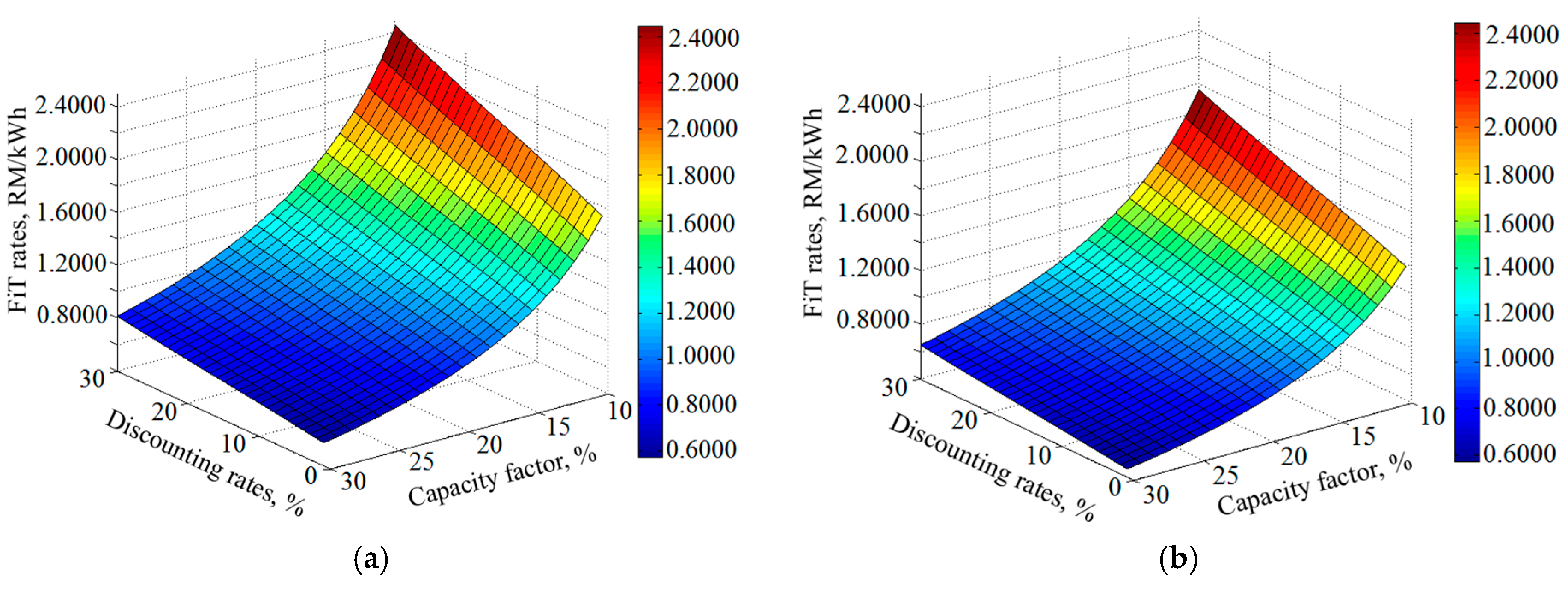
Figure 3.
Map of Sabah and selected case study site in Bak-bak, Kudat, eastern Malaysia [45].
Figure 3.
Map of Sabah and selected case study site in Bak-bak, Kudat, eastern Malaysia [45].

Table 1.
The cash inflow and cash outflow components of a cost-based tariff model for onshore wind energy generation in Malaysia.
Table 1.
The cash inflow and cash outflow components of a cost-based tariff model for onshore wind energy generation in Malaysia.
| Components | Parameters | Equations |
|---|---|---|
| Cash inflow | The after-tax income from the produced energy | |
| The capital allowance | ||
| Cash outflow | The share of equity from CAPEX | |
| The debt repayment | ||
| WT component replacement cost | ||
| Operation and maintenance cost, OPEX |
Table 2.
Estimation of economic parameters used in the calculation of baseline FiT rates for wind energy in Malaysia.
Table 2.
Estimation of economic parameters used in the calculation of baseline FiT rates for wind energy in Malaysia.
| Parameters | Symbol | Estimated Value | Reference |
|---|---|---|---|
| Baseline capacity factor | CF | 20% | [36] |
| Annual energy degradation, % | γ | 1.6% | [18] |
| Share of equity, % | θ | 20% | [20] |
| Share of debt, % | (1 − θ) | 80% | [20] |
| Maturity of loan, years | M | 15 years | [39] |
| REPPA | N | 21 years | [42] |
| Payment interest rate, % | r | 5% | [39] |
| Corporate tax, % | 25% | [17] | |
| Discount rates, % | i | 5.81% | See in Section 3.5 |
Table 3.
The impact of investment cost on the FiT rates for wind energy in Malaysia.
| Scenario | Increment or Decrement of Investment Cost | The Amount of Investment Cost, RM/kWh | Baseline FiT Rates, RM/kWh | |
|---|---|---|---|---|
| WITH Capital Allowance | WITHOUT Capital Allowance | |||
| Wind park with small-scale wind turbines | +30% | 18,750 | 1.3868 | 1.6969 |
| +20% | 15,000 | 1.1094 | 1.3575 | |
| +10% | 13,750 | 1.0170 | 1.2444 | |
| 0% | 12,500 | 0.9245 | 1.1313 | |
| −10% | 11,250 | 0.8321 | 1.0181 | |
| −20% | 10,000 | 0.7396 | 0.9050 | |
| −30% | 8750 | 0.6472 | 0.7919 | |
| Wind park with utility-scale wind turbines | +30% | 13,000 | 0.9615 | 1.1765 |
| +20% | 12,000 | 0.8875 | 1.0860 | |
| +10% | 11,000 | 0.8136 | 0.9955 | |
| 0% | 10,000 | 0.7396 | 0.9050 | |
| −10% | 9000 | 0.6657 | 0.8145 | |
| −20% | 8000 | 0.5917 | 0.7240 | |
| −30% | 7000 | 0.5177 | 0.6335 | |
Table 4.
The mean values of wind speed and Weibull parameters at the case study site.
| Height (m) | Mean Value of Wind Speed, (m/s) | Weibull Shape Parameter, k | Scale Parameter, c (m/s) |
|---|---|---|---|
| 70 | 5.90 | 2.22 | 6.70 |
| 50 | 5.40 | 2.15 | 6.10 |
| 35 | 4.80 | 2.06 | 5.40 |
| 10 | 2.90 | 1.87 | 3.30 |
Table 5.
The wind turbine specifications, wind farm layout and energy production for all wind turbines in a 1 km2 land area, Kudat, Eastern Malaysia.
Table 5.
The wind turbine specifications, wind farm layout and energy production for all wind turbines in a 1 km2 land area, Kudat, Eastern Malaysia.
| Components | Information | Deimos 60 kW | Suzlon 950 kW |
|---|---|---|---|
| Wind turbine specifications | Hub height (m) | 60.0 | 65.0 |
| Rotor diameter (m) | 21.0 | 64.0 | |
| Cut-in wind speed (m/s) | 3.0 | 3.0 | |
| Rated wind speed (m/s) | 10.0 | 11.0 | |
| Wind farm layout | Optimal number of wind turbines | 95 | 12 |
| Wind turbine distance | 5 rotor diameter | 5 rotor diameter | |
| Energy analysis | Gross annual energy production, MWh/year | 16,087.2 | 23,521.6 |
| Gross capacity factor, % | 32.22 | 23.55 | |
| Net annual energy production, MWh/year | 13,833.4 | 21,694.8 | |
| Net capacity factor, % | 27.70 | 21.72 |
Table 6.
The economic metrics analysis of optimal number of two models of wind turbines that are placed in 1 km2 area, Kudat, Eastern Malaysia.
Table 6.
The economic metrics analysis of optimal number of two models of wind turbines that are placed in 1 km2 area, Kudat, Eastern Malaysia.
| Wind Turbines and Capacity Factors | Feed-In Tariff Rates | Simple Payback Period, Years | Discounted Payback Period, Years | Project IRR (Without Debt), % | Equity IRR (With 80% Debt), % | |||
|---|---|---|---|---|---|---|---|---|
| A | B | A | B | A | B | |||
| Small scale wind turbine, Deimos 60 kW, CF: 27.70% | FiT rate generated with capital allowance, 0.9245 RM/kWh | 8.16 | 2.60 | 13.15 | 9.78 | 6.56 | 34.26 | 12.57 |
| FiT rate generated without capital allowance, 1.1313 RM/kWh | 6.67 | 1.73 | 3.94 | 13.70 | 10.27 | 53.25 | 27.06 | |
| Utility scale wind turbine, Suzlon 950 kW, CF: 21.72% | FiT rate generated with capital allowance, 0.7396 RM/kWh | 10.41 | 5.03 | >21 | 5.56 | <0.00 | 12.38 | <0.00 |
| FiT rate generated without capital allowance, 0.9050 RM/kWh | 8.51 | 2.86 | 16.17 | 9.03 | 5.85 | 30.49 | 10.41 | |
A: closed-form equation that includes the CA; B: closed-form equation that excludes the CA.
© 2017 by the authors. Licensee MDPI, Basel, Switzerland. This article is an open access article distributed under the terms and conditions of the Creative Commons Attribution (CC BY) license (http://creativecommons.org/licenses/by/4.0/).
Share and Cite
MDPI and ACS Style
Albani, A.; Ibrahim, M.Z.; Taib, C.M.I.C.; Azlina, A.A. The Optimal Generation Cost-Based Tariff Rates for Onshore Wind Energy in Malaysia. Energies 2017, 10, 1114. https://doi.org/10.3390/en10081114
AMA Style
Albani A, Ibrahim MZ, Taib CMIC, Azlina AA. The Optimal Generation Cost-Based Tariff Rates for Onshore Wind Energy in Malaysia. Energies. 2017; 10(8):1114. https://doi.org/10.3390/en10081114
Chicago/Turabian StyleAlbani, Aliashim, Mohd Zamri Ibrahim, Che Mohd Imran Che Taib, and Abd Aziz Azlina. 2017. "The Optimal Generation Cost-Based Tariff Rates for Onshore Wind Energy in Malaysia" Energies 10, no. 8: 1114. https://doi.org/10.3390/en10081114
Note that from the first issue of 2016, this journal uses article numbers instead of page numbers. See further details here.