A Current Frequency Component-Based Fault-Location Method for Voltage-Source Converter-Based High-Voltage Direct Current (VSC-HVDC) Cables Using the S Transform

Abstract

This paper proposes a fault-location method for voltage-source converter (VSC)-based high-voltage direct current (VSC-HVDC) systems. This method relies on the current frequency components generated by faults in the cable, and requires the arrival time of the frequency components at two terminals. The S transform is a time–frequency analysis tool that is superior to the wavelet transform in some respects. Therefore, the S transform was employed to determine the arrival time in this paper. To obtain a reliable criterion, a novel phase-mode transform method for bipolar cables was developed, and the propagation characteristics of the current frequency components through out the cable were analyzed. A two-terminal VSC-HVDC system was modeled in power system computer aided design/electromagnetic transients including DC (PSCAD/EMTDC). Various faults under different conditions were simulated on the basis of this model, and the simulation results verified a high accuracy, robustness against fault-resistance, and noise immunity of the proposed method.

1. Introduction

Voltage-source converter (VSC)-based high-voltage direct current (VSC-HVDC) is a new transmission technology based on voltage-source converter topologies and fully-controlled semiconductors. It can address not only conventional network issues, but also niche markets, such as the integration of large-scale renewable energy sources with the grid and large onshore/offshore wind farms [1,2]. Additionally, VSC-HVDC has the benefit of flowing a bi-directional power flow with ease, and possesses the ability to create an electrical network [3]. The faults in DC cables may cause great damage to the VSC-HVDC system. To ensure a safe DC fault extinguishment for VSC-HVDC systems, a precise determination of the fault location is required.

The current fault-location techniques are mostly based on traveling wave theory [4,5]. The accuracy of the traveling wave-based fault-location methods is high. However, the feasibility of these methods depends on the detection of the wave heads at the terminals of the transmission line. If the measurements at the terminals of the transmission line fail to identify the wave heads, the methods will be ineffective. To identify the wave head successfully, a high sampling frequency of data and experienced technicians are required. Additionally, the traveling wave, after a DC fault with a large fault resistance, is weak, and sometimes cannot be captured successfully. The wavelet transform has the capability of time location and frequency location simultaneously during the signal analysis [6,7]; thus, it is widely employed to detect the wave head. Many fault-location methods based on the wavelet transform are proposed [8,9,10].

Some fault-location methods based on time-domain analysis have also been proposed. A fault-location method for transmission lines using synchronized voltage measurements at both endings of the line is described in [11]. Reference [12] proposes a fault-location method for VSC-HVDC system transmission lines using an active impedance estimation technique. A fault-location method is proposed in [13], which estimates the fault distance on the basis of the similarity of the post-fault voltage signal to existing patterns. The fault-location algorithms proposed in [14] are based on the distributed parameter model of the transmission line. An electrical circuit parameter evaluation-based fault-location method for VSC-HVDC cables is proposed in [15]. The time-domain fault-location methods can satisfy the system’s demand of a high reliability, but the accuracy of these methods is not as high as the traveling wave-based fault-location methods.

The wavelet transform has made a great contribution to traveling wave-based fault-location techniques. However, different types of signals require different wavelet bases, and it is not easy to select a proper wavelet basis. The S transform was proposed by R. G. Stockwell in 1996 [16]. It is a time–frequency analysis tool that is an extension of the wavelet and Fourier transforms. The S transform can overcome the shortcomings of the wavelet transform, and additionally, its transform result for the transient signal is more intuitive. In recent years, the S transform has been applied in many references for power quality detection [17,18,19,20]. A fault-location method for AC transmission lines using the S transform is proposed in [21]. However, the fault-location method for VSC-HVDC cables employing the S transform has not been mentioned before. In this paper, a current frequency component-based fault-location method for VSC-HVDC cables using the S transform is proposed. The feasibility and applicability of the proposed fault-location method are researched deeply. The characteristics of the traveling-wave in the DC cable are greatly different to those in the AC transmission line. To obtain a reliable criterion for the proposed fault-location method, a phase-mode transform method for bipolar DC cables was developed, and the propagation characteristics of the current frequency components in the cable were analyzed in detail.

In this paper, a brief introduction of the S transform is given in Section 2, and the fault-location principle is described. In Section 3, a phase-mode transform method for bipolar DC cables is proposed, and the propagation characteristics of the current frequency components are represented. On the basis of the analysis, a fault-location method employing the S transform for VSC-HVDC cables is proposed in Section 4. In Section 5, the numerical simulation results and discussion based on a test system are presented. Finally, a summary of the main conclusion and contributions of the paper are presented in Section 6.

2. Fault-Location Principle

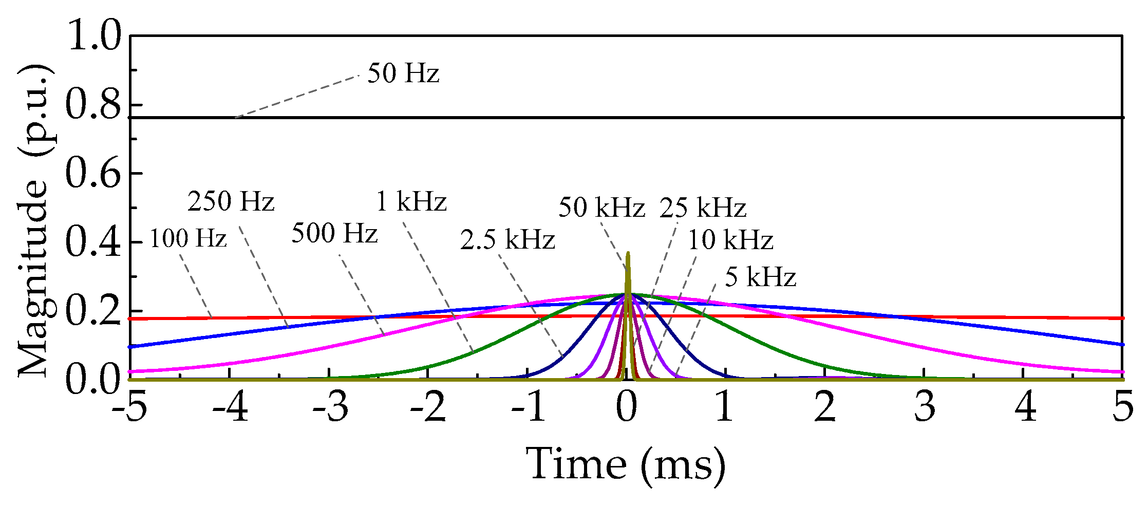
2.1. Brief Introduction of the S Transform

The S transform of a signal x(t) is expressed as [16]

$$\{\begin{array}{l}S(\tau ,f)={\displaystyle {\int }_{-\infty }^{+\infty }x(t)\omega (\tau -t,f)e^{-i2\pi f\tau }dt}\\ \omega (\tau -t,f)=\frac{\left|f\right|}{\sqrt{2\pi }}{e}^{-\frac{f^2{(\tau -t)}^2}{2}}\end{array}$$

(1)

where ω(τ−t, f) is the Gaussian window function with a time-shift factor of τ and a frequency of f. As shown in Equation (1), the S transform is a time–frequency analysis tool, which can be derived from the continuous wavelet transform (CWT) and the short-time Fourier transform (STFT).

The S transform of a discrete signal x[jT] is realized by the fast Fourier transform (FFT), and is expressed as [16]

$$\{\begin{array}{l}S[kT,\frac{n}{NT}]={\displaystyle \sum _{m=0}^{N-1}X[\frac{m+n}{NT}]e^{\frac{-2{\pi }^2{m}^2}{n^2}}{e}^{\frac{i2\pi mk}{N}},n\ne 0}\\ S[kT,0]=\frac{1}{N}{\displaystyle \sum _{m=0}^{N-1}X[\frac{m}{NT}],n=0}\end{array}$$

(2)

where $k,m,n\in (0,N-1)$. N is the sampling number, and T is the sampling interval. X[n/NT] is the discrete Fourier transform of x[jT], and $e^{-2{\pi }^2{m}^2/n^2}$ is the Fourier spectrum of the Gaussian window function.

As seen from Equation (2), the S transform result of a discrete signal is a complex matrix. A row vector of the matrix represents the frequency-magnitude characteristic of the signal at a specific moment, and the frequency interval is 1/NT, denoted by f₀. A column vector represents the time-magnitude characteristic of a frequency component with a specific frequency, and the time interval is T. For example, we denote the S transform result by S, and S[k + 1, n + 1] represents the frequency component with a frequency of nf₀ at the time kT.

The wavelet transform provides a cogent math tool for transient signal analysis. However, the wavelet transform results for a signal may be different under different wavelet bases and scales; thus, it is imperative to select the proper wavelet basis and scale for a specific signal. The Fourier transform has a window with a fixed height and width; thus, it cannot adjust the time–frequency resolution with variations of the time and frequency. The S transform inherits the advantages of the wavelet transform and the Fourier transform, and can overcome both of their shortcomings. The S transform is perfectly reversible. The phase of the S transform referenced to the time origin provides useful and supplementary information regarding spectra that is not available from locally referenced phase information in the wavelet transform [16]. By means of the S transform, all the frequency components with a frequency interval of f₀ can be extracted, and the proper frequency components can be selected conveniently. Additionally, the S transform results are more intuitive than the wavelet transform results, which will be discussed in detail in Section 5.7. The height and width of the Gaussian window can change with a variation of the frequency; thus, the S transform can adjust its time and frequency resolution ability with respect to the frequency.

In this paper, the S transform was realized by means of matrix laboratory (MATLAB). We take a series of signals that contained fault data at 0 ms as an example. The frequency components of the signal were extracted by the S transform, and the time-magnitude curves of some typical frequency components are shown in Figure 1. As can be seen, when the frequency is lower than 500 Hz, the time-magnitude curves of the frequency components are smooth, but they are different from each other. This indicates that, in the low-frequency range, the frequency resolution ability of the S transform is remarkable, whereas the time resolution ability is not very good. When the frequency is greater than 2.5 kHz, the time-magnitude curves are concentrated at the fault time; thus, the transient fault signal can be represented intuitively. This indicates that the time resolution ability of the S transform is improved in the high-frequency range. For fault identification and location, a good time resolution ability is more critical. Therefore, due to the satisfactory time resolution ability of the S transform in the high-frequency range, the high-frequency components were employed for fault location in this paper.

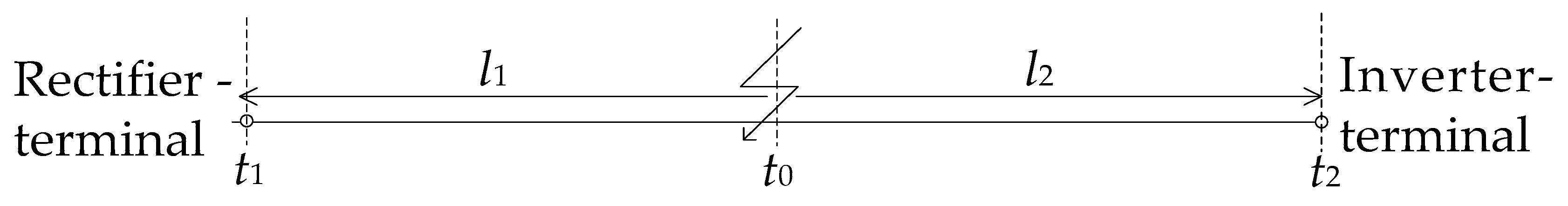
2.2. Estimation of the Fault Distance

After the occurrence of a fault in the DC cable, the fault current frequency components at the fault point start traveling toward both terminals. Assuming a fault occurs in the cable at a time t₀, shown in Figure 2, and the fault point is at a distance l₁ from the rectifier-terminal and a distance l₂ from the inverter-terminal, for a fault frequency component with a specific frequency, if the frequency component arrives at the rectifier-terminal at a time t₁ and at the inverter-terminal at a time t₂, the fault time can be calculated as

$$t_0=\frac{(t_1+t_2-\frac{L}{v})}{2}$$

(3)

where v is the propagation velocity of the frequency component, and L is the total length of the cable. Thus, the distance between the fault point and the rectifier-terminal can be calculated as

$$l_1=v(t_1-t_0)$$

(4)

As seen from Equations (3) and (4), to estimate the fault distance, the arrival time and propagation velocity of the frequency component should be obtained.

3. Analysis of the Current Frequency Components

As can be seen from Equations (3) and (4), the proposed fault-location method is based on the current frequency components in the DC cable. To obtain a convincing criterion, the characteristics of the current frequency components should be analyzed first. We take a VSC-HVDC system as an example, whose schematic is shown in Figure 3. The two VSC stations are connected with a bipolar cable. The AC systems connected to VSC1 and VSC2 are modeled by two 420 kV generators. On the DC side, p1, p2, n1 and n2 are four relays taken as protection devices for the cables.

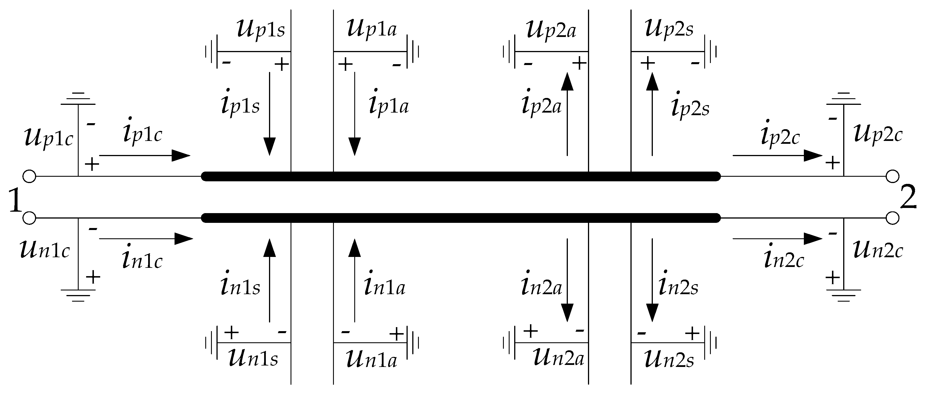
3.1. Phase-Mode Transform Method for Bipolar Cables

The cross section of a bipolar DC cable is shown in Figure 4. A single cable is composed of three layers from the inner to the outside: a conductor layer, a sheath layer and an armor layer. Therefore, for a bipolar cable, there are six sets of parameters, which are coupled with each other; thus, it is necessary to decouple the parameters of the cable. The decoupling methods for the three-phase AC cable are represented in [22,23]. Similarly, the decoupling method for the bipolar DC cable can be derived; it is described in this subsection.

The schematic diagram of the bipolar DC cable is shown in Figure 5. The output terminal of the rectifier station is denoted by 1 and the output terminal of the inverter station is denoted by 2. Taking terminal 1 as an example, the DC voltages of the conductor layer, shielding layer and armor layer for the positive cable are denoted by u_p1c, u_p1s and u_p1a, respectively. The DC voltages of the three layers for the negative cable are denoted by u_n1c, u_n1s and u_n1a, respectively. The DC currents of the six layers at terminal 1 are denoted by i_p1c, i_p1s, i_p1a, i_n1c, i_n1s and i_n1a, respectively.

Defining R, L, G and C as the matrices of the resistance, inductance, conductance and capacitance per meter of the DC cable, respectively, then the wave equations with mutual inductance can be represented as follows [22]:

$$\{\begin{array}{l}\frac{\partial U_1}{\partial x}=-R{I}_1-L\frac{\partial I_1}{\partial t}\\ \frac{\partial I_1}{\partial x}=-G{U}_1-C\frac{\partial U_1}{\partial t}\end{array}$$

(5)

where U₁ = [u_p1c, u_n1c, u_p1s, u_n1s, u_p1a, u_n1a], and I₁ = [i_p1c, i_n1c,i_p1s, i_n1s, i_p1a, i_n1a]. The key to realizing the decoupling is to transform R, L, G and C to diagonal matrices. According to this principle, the phase-mode transform matrix of DC voltages can be derived and represented as follows:

$$P=k\otimes \left[\begin{array}{lll}I\hfill & I\hfill & I\hfill \\ I\hfill & I\hfill & 0\hfill \\ I\hfill & 0\hfill & 0\hfill \end{array}\right]$$

(6)

where 0 and I are the two-dimensional zero matrix and unit matrix, respectively, while k is the Karenbauer transform matrix, expressed as

$$k=\left[\begin{array}{cc}\hfill 1& \hfill 1\\ \hfill 1& \hfill -1\end{array}\right]$$

(7)

Introducing Q = P^−T as the phase-mode transform matrix of DC currents, then Equation(5) can be transformed to

$$\{\begin{array}{l}\frac{\partial U_{1m}}{\partial x}=-P^{-1}RQ{I}_{1m}-P^{-1}LQ\frac{\partial I_{1m}}{\partial t}\\ \frac{\partial I_{1m}}{\partial x}=-Q^{-1}GP{U}_{1m}-Q^{-1}CP\frac{\partial U_{1m}}{\partial t}\end{array}$$

(8)

where I_1m is expressed as

$$I_{1m}=Q^{-1}{I}_1=\left[\begin{array}{l}{i}_{p1c}+i_{n1c}+i_{p1s}+i_{n1s}+i_{p1a}+i_{n1a}\\ i_{p1c}-i_{n1c}+i_{p1s}-i_{n1s}+i_{p1a}-i_{n1a}\\ i_{p1c}+i_{n1c}+i_{p1s}+i_{n1s}\\ i_{p1c}-i_{n1c}+i_{p1s}-i_{n1s}\\ i_{p1c}+i_{n1c}\\ i_{p1c}-i_{n1c}\end{array}\right]$$

(9)

Through the operation above, the currents in the bipolar cable can be transformed to six independent mode currents. In the following, the current I_1m[p] is denoted as the pth mode current, where p = 1, 2, …, 6.

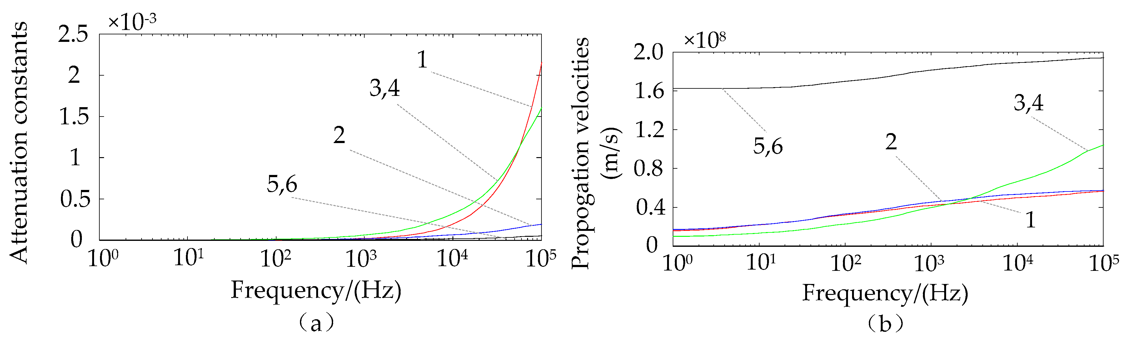
3.2. Propagation Characteristics of the Current Frequency Components

The attenuation constant matrix of the mode currents through the cable can be obtained as [22]

$$A=real(\sqrt{Z_m{Y}_m})$$

(10)

where Z_m and Y_m are the impedance matrix and admittance matrix after decoupling, and real() is the function to extract the real part of a complex number. It is easy to see that A[p, p] is the attenuation constant of the pth mode current.

As seen from Equation (8), the resistance, inductance, conductance and capacitance matrices after decoupling are expressed as R_m = Q^TRQ, L_m = Q^TLQ, G_m = P^TGP and C_m = P^TCP, respectively. Denoting R_m[p, p], L_m[p, p], G_m[p, p] and C_m[p, p] by R_p, L_p, G_p and C_p, respectively, then the propagation velocity of the pth mode current can be calculated as [22]

$$v_p=\frac{\omega }{\sqrt{\frac{1}{2}\left[{\omega }^2{L}_p{C}_p-R_p{G}_p+\sqrt{\left(R_p^2+{\omega }^2{L}_p^2\right)\left(G_p^2+{\omega }^2{C}_p^2\right)}\right]}}$$

(11)

where ω is the angular velocity.

Figure 6a,b shows the attenuation constants and propagation velocities of the mode currents with respect to the frequency, respectively. In Figure 4, the line marked as “p” represents the attenuation constant or the propagation velocity of the pth mode current, where p = 1, 2, …, 6. As seen from Figure 6a, the attenuation constants of the fifth and sixth mode currents stay low with the increase of the frequency, while the attenuation constants of the other mode currents increase markedly. As seen from Figure 6b, the velocities of the fifth and sixth mode currents are close to that of the traveling wave through the DC cable when the frequency is higher than 5 kHz, whereas the velocities of the other mode currents are significantly lower. According to Equations (3) and (4), although influenced by the high propagation velocity, the fault-location accuracy can be improved by increasing the sampling rate of the current signal. However, if the attenuation constant is too large, the fault current signal will be too weak to be detected, and thus the fault-location method will fail. Therefore, the fifth and sixth mode currents are more suitable for fault location. According to the reference direction of the currents, as in Figure 5, the sixth mode current was selected as the fault-location parameter in this paper. To obtain the sixth mode current, the currents of the conductor layers in both poles are needed, as in Equation (9).

4. Fault-Location Method

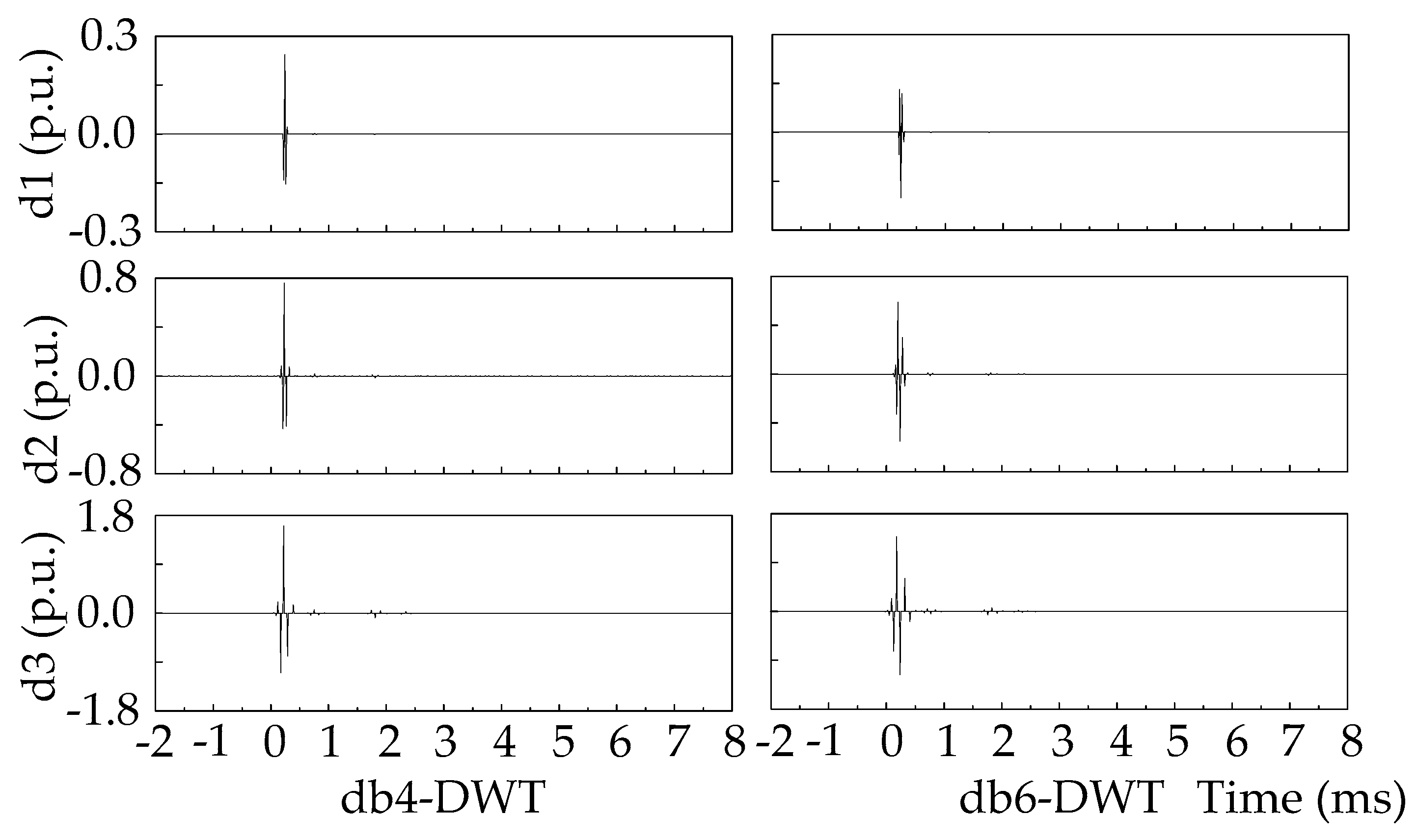
4.1. Extraction and Processing of Frequency Components

It has been mentioned in Section 2 that the time resolution ability of the S transform significantly improves with an increase of the frequency. According to Figure 1, when the frequency is higher than 10 kHz, the time resolution ability of the S transform is satisfactory. Additionally, as seen from Figure 6b, the velocities of the frequency components (10–20 kHz) of the sixth mode current are close to each other; thus, it can be considered that they arrive at one of the cable terminals at the same time. Due to the analysis above, the frequency components (10–20 kHz) of the sixth mode current were selected for fault location in this paper. By means of the S transform, the time-magnitude characteristic of the frequency components (10–20 kHz) of the sixth mode current at the cable terminals can be extracted. Denoting the summation of their magnitudes at the time kT as M, then M is expressed as

$$M={\displaystyle \sum _{n_1\le n\le n_2}abs(S_6(k+1,n+1))}$$

(12)

where the matrix S₆ is the S transform result of the sixth mode current signals, and n₁f₀ = 10 kHz and n₂f₀ = 20 kHz.

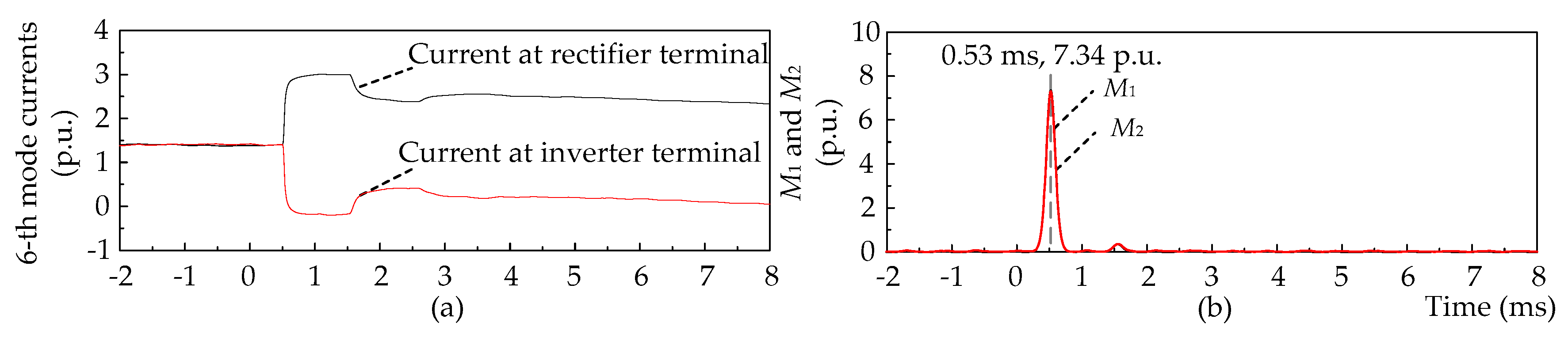
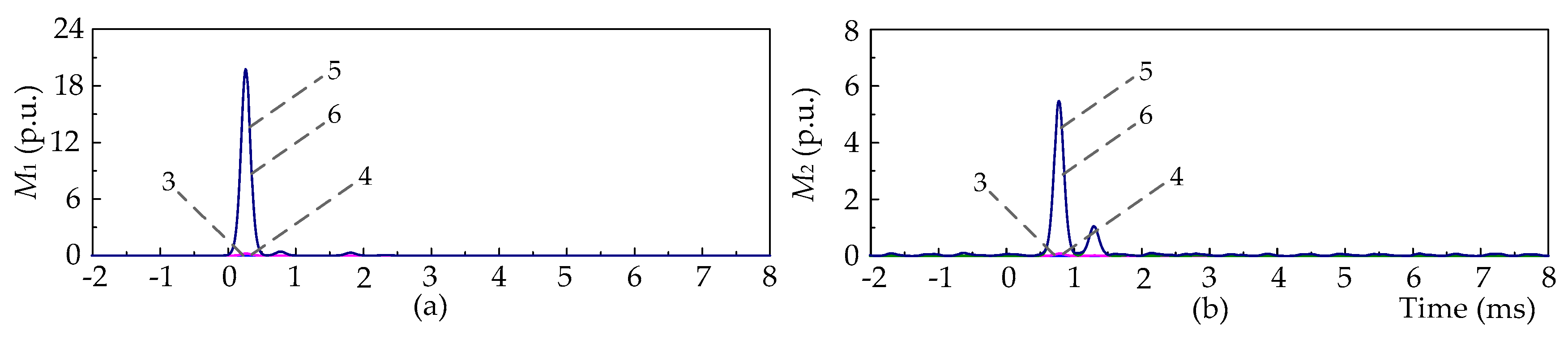
4.2. Determination of the Arrival Time

When the fault frequency components (10–20 kHz) first arrive at the cable terminals, they will cause the first sudden change points of M. Therefore, according tothe first sudden change point of M, the first arrival time of the frequency components can be determined. The sudden change point of M can be extracted through the following equation:

$$\{\begin{array}{l}\frac{dM}{dt}>0,t<t_m\\ \frac{dM}{dt}<0,t>t_m\end{array},\mathrm{and}M(t_m)>M_h$$

(13)

where t_m is the sudden change time of M, and M_h is the threshold value of M to avoid the influence of disturbances. The first sudden change point of M can be determined easily because its magnitude is usually much higher than those of the subsequent change points.

We denote the sixth mode currents at the rectifier-terminal and inverter-terminal by i_1m6 and i_2m6, respectively. The value of M calculated from i_1m6 is denoted by M₁, and the value of M calculated from i_2m6 is denoted by M₂. The arrival timest₁ and t₂ can be obtained through the first sudden change points of M₁ and M₂, respectively.

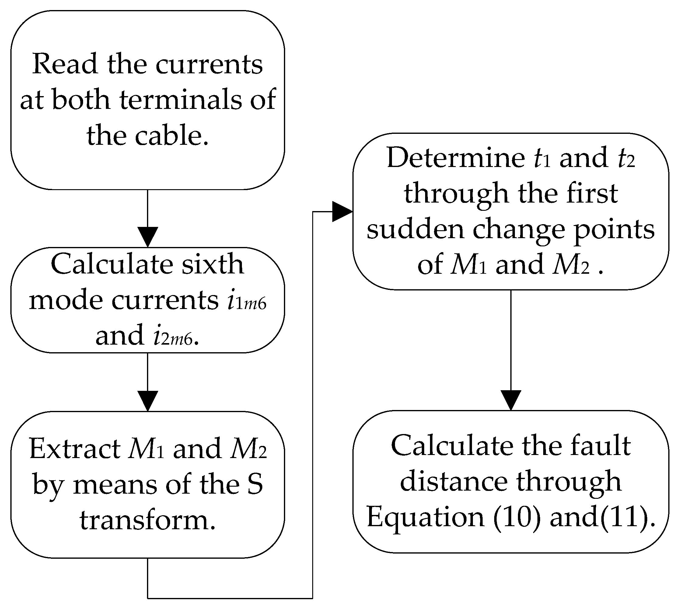
4.3. Flow Chart of the Fault-Location Method

After determining the arrival timest₁and t₂, the fault distance can be estimated through Equations (3) and (4). The propagation velocities of the frequency components (10–20 kHz) can be obtained from Figure 6, and their average value is considered as the velocity v in Equations (3) and (4). The flow chart of the fault-location method is shown in Figure 7. The fault-location method is simple but efficient.

The fault-location error is defined as

$$Error=\frac{\left|l_1-l_{1act}\right|}{L}\times 100\%$$

(14)

where l_1act is the actual distance between the fault point and rectifier-terminal. The fault-location error is mainly influenced by the sampling rate and calculation error.

5. Test System and Simulation Results

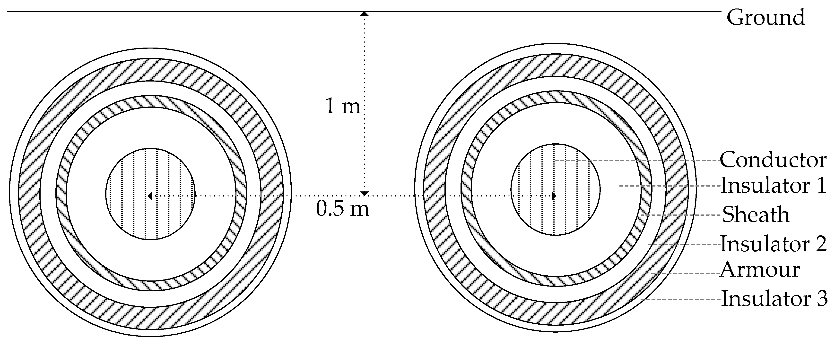
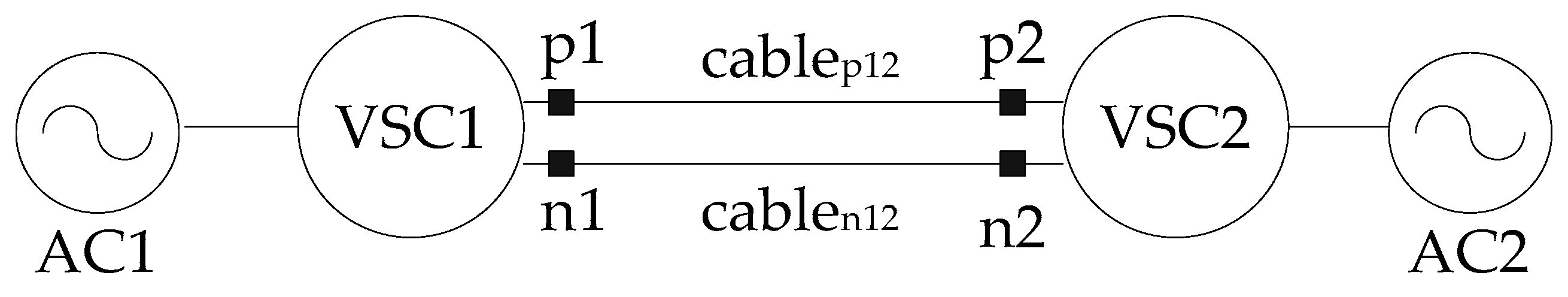
5.1. Test System

The VSC-HVDC system in Figure 3 was established using a power system computer-aided design/electromagnetic transients including DC (PSCAD/EMTDC). The DC cable was modeled by a frequency-dependent model, and its total length L was 200 km. Some typical faults were simulated in this model to verify the proposed fault-location method. The internal positive-cable-to-ground (PG) faults and positive-cable-to-negative-cable (PN) faults were simulated in the system. The occurrence time for all the faults in the following was set to 0 ms. The unit of the current was per unit (p.u).

5.2. Testof the Determination Method of theArrival Time

Many simulations were performed to verify the accuracy of the determination of t₁ and t₂. Figure 8 shows the curves of the sixth mode currents at the two terminals of the cable and the corresponding M₁ and M₂ during the PG fault at the middle point of the cable with a fault resistance of 100 Ω. As shown in the figure, the curves of M₁ and M₂ almost overlap, and they both reached the first sudden change points 0.53 ms after the occurrence of the fault; this time is equal to L/2v. This indicates that the arrival timest₁ and t₂ can be determined accurately through the sudden change points of M₁ and M₂.

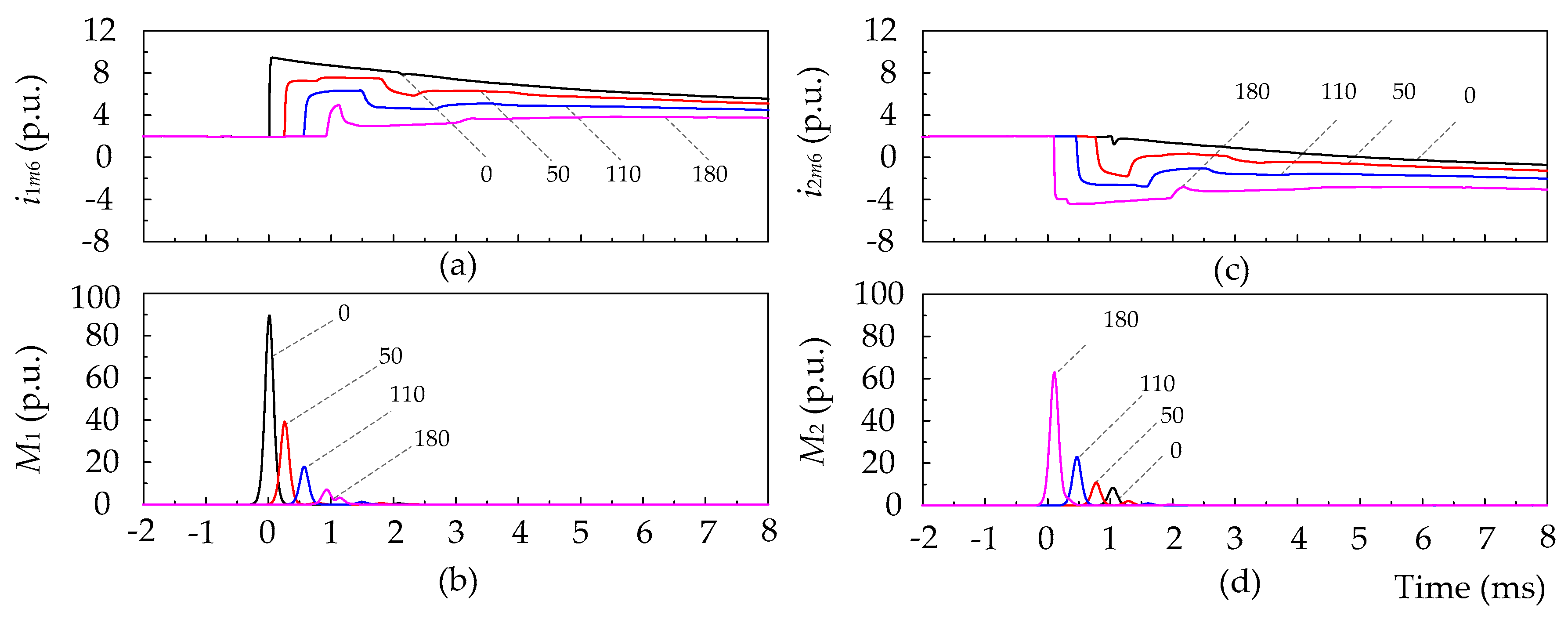
5.3. Fault-Location Results

A number of PG faults 50 km from the rectifier-terminal were simulated. The fault resistance took the values of 0, 25, 50, …, 500 Ω. The sampling rate was set to 100 kHz. To provide the details, the currents of the conductor layers at p1, n1, p2 and n2 during the faults are displayed in Figure 9. The sixth mode DC currents at the two terminals of the cable were calculated according to the currents in Figure 9, and the corresponding M₁ and M₂ during the faults were plotted and are displayed in Figure 10a,b. The numbers of the lines in the figures represent the fault resistances (Ω) of the faults. As seen from Figure 9, there were oscillations in the currents when the fault resistance was small, and with the increase of the fault resistance, the change rates and change values of the currents decreased markedly. As seen from Figure 10, for each of the faults, the first sudden change points of M₁ and M₂wereprominent and sharp, while their sudden change times were not influenced by the oscillations of the currents or the fault resistance. When the fault resistance was0 Ω, the peak values of the sudden change points of M₁ and M₂ were nearly 190 p.u., and when the fault resistance was 500 Ω, the peak values of the sudden change points of M₁ and M₂ were about 4.4 p.u. In general, the peak values of the sudden change points of M₁ and M₂ decreased gradually with the increase of the fault resistance. However, they were large enough to be observed even when the fault resistance was very large.

The simulation results for some PG faults are displayed in

Table 1. Fault-location results for various PG faults.

Fault Distance (km)	Fault Resistance (Ω)	t1 (ms)	t2 (ms)	Estimated Distance (km)	Fault-Location Error (%)
0	0	0.01	1.03	1.7897	0.8948
	100	0.01	1.04	0.8268	0.4134
	500	0.01	1.04	0.8268	0.4134
50	0	0.26	0.78	49.932	0.3402
	100	0.26	0.78	49.932	0.3402
	500	0.26	0.78	49.932	0.3402
110	0	0.57	0.47	109.63	0.1857
	100	0.57	0.47	109.63	0.1857
	500	0.57	0.47	109.63	0.1857
180	0	0.93	0.11	178.95	0.5233
	100	0.93	0.11	178.95	0.5233
	500	0.93	0.11	178.95	0.5233

.The fault distance between the fault point and the rectifier-terminal took the values of 0, 50, 110 and 180 km, whereas the fault resistance took the values of 0, 100 and 500 Ω. The obtained terminal current signals were sampled with a sampling rate of 100 kHz. To provide the details, the detected arrival time, estimated distance between the fault point and rectifier-terminal and the fault-location error are displayed in Table 1. As shown in Table 1, the minimum fault-location error was 0.1857% and the maximum fault-location error was 0.8948%.

Various PN faults with a fault resistance of 100 Ω were simulated. The distance between the fault point and the rectifier-terminal varied from 0 to 180 km. The obtained terminal current signals were sampled with a sampling rate of 100 kHz. Figure 11 shows the curves of the sixth mode currents i_1m6 and i_2m6 and the corresponding M₁ and M₂. The numbers of the lines in Figure 11 represent the distance (km) between the fault point and rectifier-terminal. As can be seen, for each of the faults, the first sudden change points of M₁ and M₂ can be extracted easily and can exactly represent the sudden change of the currents.

Table 2. Fault-location results for PN faults with a fault resistance of 100 Ω at different locations.

Fault Distance (km)	t1 (ms)	t2 (ms)	Estimated Distance (km)	Fault-Location Error (%)
0	0.01	1.04	0.8268	0.4134
50	0.26	0.78	49.932	0.3402
110	0.57	0.47	109.63	0.1857
180	0.93	0.11	178.95	0.5233

shows the detected arrival time, the estimated distance between the fault point and rectifier-terminal and the fault-location error for the PN faults. As shown in Table 2, the minimum fault-location error was 0.1857% and the maximum fault-location error was 0.5233%.

The simulation results in Table 1 and Table 2 show that with a sampling rate of 100 kHz, the fault distance can be estimated accurately by the proposed fault-location method.

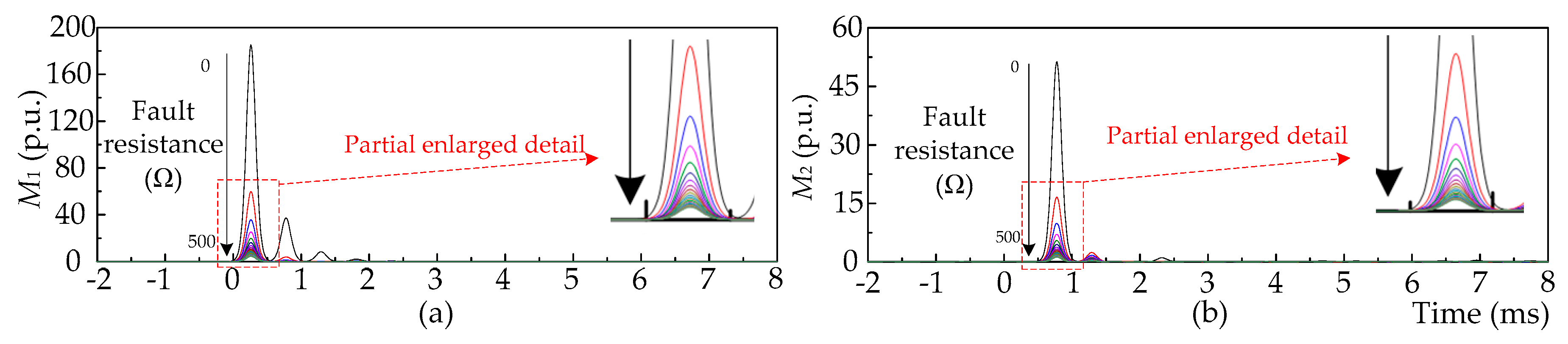
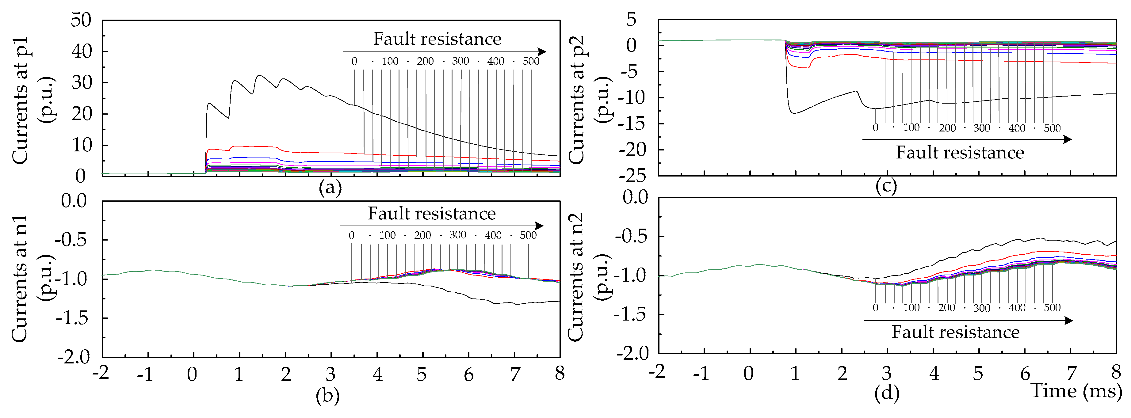
5.4. Influence of the Fault Resistance

It can be seen from Table 1 and Table 2 that the accuracy of the proposed fault-location method is not sensitive to the fault resistance. Figure 10 shows that with an increase of the fault resistance, the peak values of the sudden change points of M₁ and M₂ decrease gradually. However, the peak values of the sudden change points of M₁ and M₂ are both significantly large, even when the fault resistance is 500 Ω. This indicates that the proposed fault-location method is not vulnerable to a large fault resistance.

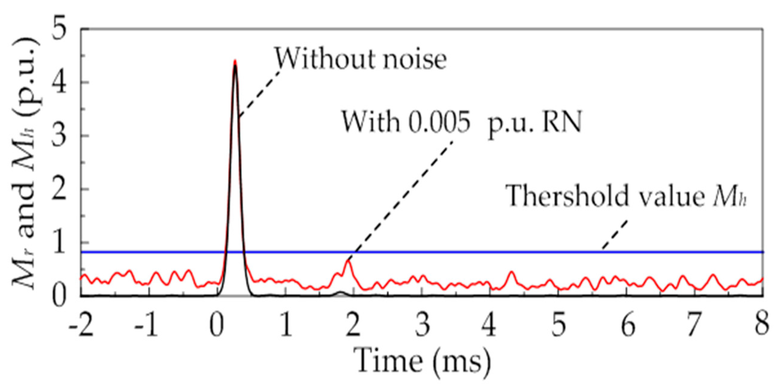
5.5. Influence of Noise

To investigate the influence of noise on the proposed fault-location method, the obtained current signals were contaminated with 0.005 p.u. of random noise (RN). For the PG fault 50 km from the rectifier-terminal with a fault resistance of 500 Ω, the noise was added to the rectifier-terminal currents. The curves of M₁ are displayed in Figure 12. As seen from the figure, the noise could also cause the sudden change points of M₁, but the magnitudes of the sudden change points caused by noise were much lower than those caused by faults. Therefore, a threshold M_h was set to reject the sudden change points that were associated to noise, as shown in Figure 12. The threshold M_h in Figure 12 is smaller than 1 p.u., and it is much smaller than the peak value of the sudden change point of M₁ caused by faults. Therefore, the noise can be ignored effectively by setting a threshold M_h.

For more detailed study, various PG faults were simulated and the 0.005p.u. of RN was added to the current signals. The fault distance between the fault point and the rectifier-terminal took the values of 0, 50, 110 and 180 km, and the fault resistance was set to500Ω. The obtained terminal current signals were sampled with a sampling rate of 100 kHz. The fault-location errors are displayed in

Table 3. Fault-location errors for PG faults at various locations with a fault resistance of 500 Ω, considering the influence of noise.

Fault Distance (km)	0	50	110	180
Fault-Location Error (%)	0.5494	0.3402	0.2957	1.004

. As can be observed from Table 1 and Table 3, the fault-location error may increase under the condition of additive noise.

5.6. Effect of Sampling Rate

The accuracy of the fault-location method is usually influenced by the sampling rate. In the above, the sampling rate was set to 100 kHz. To investigate the effect of the sampling rate on the proposed method, the obtained current signals during various PG faults were also sampled under sampling rates of 200 and 500 kHz. The fault distance between the fault point and rectifier-terminal took the values of 0, 50, 110 and 180 km, and the fault resistance was set to 100 Ω. The fault-location errors for the faults are displayed in

Table 4. Fault-location errors for PG faults with a fault resistance of 100 Ω at different locations, considering the influence of the sampling rate.

Sampling Rate (kHz)	Fault Distance (km)
	0	50	110	180
	Maximum Fault-Location Error (%)
100	0.4134	0.3402	0.1857	0.5233
200	0.2474	0. 4154	0.0549	0.2826
500	0.0991	0.3511	0.0005	0.0716

. As shown in the table, with the increase of the sampling rate, the fault-location error decreased, in general.

5.7. Comparison to the Conventional Method

In this subsection, the fault-location method based on the discrete wavelet transform (DWT) is compared with the proposed method in this paper. It is mentioned in [24] that the db4 and db6 wavelets are the most suitable for the detection of short-time and fast high-frequency transient signals. In this case, the db4 and db6 wavelets were employed to detect the wave head.

Taking the PG fault50 km from the rectifier-terminal with a fault resistance of 100 Ω as an example, the d1, d2 and d3 DWT results for the sixth mode currents at the rectifier-terminal during the fault are shown in Figure 13. The fault was located according to the modulus maximums of the wavelet transform results, as shown in Figure 13. By comparing Figure 10 with Figure 13, the sudden change points of the S transform results are more intuitive than those of the DWT results. Additionally, the wavelet transform results of the signals under different wavelet bases are different; thus, it is imperative to choose the proper wavelet basis for a specific signal. As for the S transform, the Gaussian window function and the FFT transform can ensure the quality of the transform results for different signals.

5.8. Comparison of Simulation Results to the Other Mode Currents

In the above, the sixth mode current was employed for fault location. To provide more detail, the comparison of the fault-location results using different mode currents is discussed in this subsection. Taking the PG fault 50 km from the rectifier-terminal with a fault resistance of 100 Ω at the middle point of the cable as an example, the curves of M₁ and M₂ extracted from the third to sixth mode currents are shown in Figure 14. The numbers of the lines in the figure represent the corresponding mode currents. The values of M₁ and M₂ extracted from the first and second mode currents were too small, and they could not be displayed in the figure. It is easy to see that the frequency components of the first to fourth mode currents were too weak, and that it was hard to capture the fault signal through them. Therefore, the first to fourth mode currents are not suitable for the proposed fault-location method.

6. Conclusions

In this paper, a fault-location method for VSC-HVDC cables employing the S transform is proposed. With the proposed method, the fault distance can be determined using the current frequency components caused by the fault and the first arrival time of the frequency components at the cable terminals. By means of the S transform, the first arrival time of the current frequency components can be determined accurately. To obtain a reliable criterion, a new phase-mode transform method for the bipolar cable was developed. The characteristics of the mode currents were analyzed in detail and the high-frequency components of the sixth mode currents were selected for the proposed method.

A two-terminal VSC-HVDC system was modeled using PSCAD/EMTDC, and various faults under different conditions were simulated using this model to verify the proposed fault-location method. The simulation results showed that this method has the advantage of a high accuracy, and it is not sensitive to a large fault resistance and noise.

References

1. Flourentzou, N.; Agelidis, G. VSC-based HVDC power transmission systems: An overview. IEEE Trans. Power Electron. 2009, 24, 592–599. [Google Scholar] [CrossRef]
2. Bresesti, P.; Kling, W.L.; Hendriks, R.L. HVDC connection of offshore wind farms to the transmission system. IEEE Trans. Energy Convers. 2007, 1, 37–43. [Google Scholar] [CrossRef]
3. Muhammad, R.; Kevin, S.; Oriol, G.B. Droop control design of multi-VSC systems for offshore networks to integrate wind energy. Energies 2016, 9, 826. [Google Scholar]
4. Xie, J.; Chen, P. A traveling wave based fault locating system for HVDC transmission lines. In Proceedings of the 2006 International Conference on Power System Technology, Chongqing, China, 22–26 October 2006; pp. 1–4. [Google Scholar]
5. Girgis, A.; Hart, D.G.; Peterson, W.L. A new fault location technique for two- and three-terminal lines. IEEE Trans. Power Deliv. 1992, 7, 98–107. [Google Scholar] [CrossRef]
6. Magnago, F.H.; Abur, A. Fault location using wavelets. IEEE Trans. Power Deliv. 1998, 13, 1475–1480. [Google Scholar] [CrossRef]
7. Rajesh, K.; Yadaiah, N. Fault identification using wavelet transform. In Proceedings of the 2005 IEEE PES Transmission and Distribution, Dalian, China, 15–18 August 2005; pp. 1–6. [Google Scholar]
8. Nanayakkara, O.M.K.K.; Rajapakse, A.D.; Wachal, R. Traveling-wave-based line fault location in star-connected multiterminal HVDC systems. IEEE Trans. Power Deliv. 2012, 27, 2286–2294. [Google Scholar] [CrossRef]
9. Azizi, S.; Sanaye-Pasand, M.; Hasani, A. A traveling-wave-based methodology for wide-area fault location in multiterminal DC systems. IEEE Trans. Power Deliv. 2014, 29, 2552–2560. [Google Scholar] [CrossRef]
10. Nanayakkara, O.M.K.K.; Rajapakse, A.D.; Wachal, R. Location of DC line faults in conventional HVDC systems with segments of cables and overhead lines using terminal measurements. IEEE Trans. Power Deliv. 2012, 27, 279–288. [Google Scholar] [CrossRef]
11. Brahma, S.M.; Girgis, A. Fault location on a transmission line using synchronized voltage measurements. IEEE Trans. Power Deliv. 2004, 19, 1619–1622. [Google Scholar] [CrossRef]
12. Shukr, M.; Thomas, D.W.P.; Zanchetta, P. VSC-HVDC transmission line faults location using active line impedance estimation. In Proceedings of the 2012 IEEE International Energy Conference and Exhibition, Florence, Italy, 9–12 September 2012; pp. 244–248. [Google Scholar]
13. Farshad, M.; Sadeh, J. A novel fault-location method for HVDC transmission lines based on similarity measure of voltage signals. IEEE Trans. Power Deliv. 2013, 28, 2483–2490. [Google Scholar] [CrossRef]
14. Suonan, J.; Gao, S.; Song, G. A novel fault-location method for HVDC transmission lines. IEEE Trans. Power Deliv. 2010, 25, 1203–1209. [Google Scholar] [CrossRef]
15. Yang, J.; Fletcher, J.E.; O’Reilly, J. Short-circuit and ground fault analysis and location in VSC-based DC network cables. IEEE Trans. Ind. Electron. 2011, 59, 3827–3837. [Google Scholar] [CrossRef]
16. Stockwell, R.G.; Mansinha, L.; Lowe, R.P. Localization of the complex spectrum: The S transform. IEEE Trans. Signal. Process. 1996, 44, 998–1001. [Google Scholar] [CrossRef]
17. Lee, I.W.C.; Dash, P.K. S-transform-based intelligent system for classification of power quality disturbance signals. IEEE Trans. Ind. Electron. 2003, 50, 800–805. [Google Scholar] [CrossRef]
18. Huang, N.T.; Peng, H.; Cai, G.W. Power quality disturbances feature selection and recognition using optimal multi-resolution fast S-transform and CART algorithm. Energies 2016, 9, 927. [Google Scholar] [CrossRef]
19. Zhao, F.; Yang, R. Power-quality disturbance recognition using S-transform. IEEE Trans. Power Deliv. 2007, 22, 944–950. [Google Scholar] [CrossRef]
20. Wang, H.H.; Wang, P.; Liu, T. Power quality disturbance classification using the S-transform and probabilistic neural network. Energies 2017, 10, 107. [Google Scholar] [CrossRef]
21. Ahmadimanesh, A.; Shahrtash, S.M. Transient-based fault-location method for multiterminal lines employing S-transform. IEEE Trans. Power Deliv. 2013, 28, 1373–1380. [Google Scholar] [CrossRef]
22. Dommel, H.W. EMTP Theory Book; Bonneville Power Administration: Portland, OR, USA, 1987; pp. 150–161. [Google Scholar]
23. Chen, Y.L.; Gong, Q.W.; Chen, Y.P. Traveling wave fault location for crossbonded HV cables. High. Volt. Eng. 2008, 34, 799–803. [Google Scholar]
24. Heydt, G.T.F.; Galli, A.W. Transient power quality problems analyzed using wavelets. IEEE Trans. Power Deliv. 1997, 12, 908–915. [Google Scholar] [CrossRef]
Figure 1. The magnitude of the frequency components of a signal extracted by the S transform.
Energies 10 01115 g001
Figure 2. Propagation of the fault components.
Energies 10 01115 g002
Figure 3. Schematic of the voltage-source converter-based high-voltage direct current (VSC-HVDC) system.
Energies 10 01115 g003
Figure 4. The cross section of a DC cable.
Energies 10 01115 g004
Figure 5. The schematic diagram of the bipolar DC cable.
Energies 10 01115 g005
Figure 6. Attenuation constants and propagation velocities of the mode currents. (a) Attenuation constants. (b) Propagation velocities.
Energies 10 01115 g006
Figure 7. Flowchart of the proposed fault-location method.
Energies 10 01115 g007
Figure 8. Curves of sixth mode currents and the corresponding M1 and M2during the positive-cable-to-ground (PG) fault with a fault resistance of 100 Ω at the middle point of the cable. (a) The sixth mode currents. (b) M1 and M2.
Energies 10 01115 g008
Figure 9. The DC currents of the conductor layers during PG faults 50 km from the rectifier-terminal under different fault resistance conditions. (a) DC currents at p1. (b) DC currents at n1. (c) DC currents at p2. (d) DC currents at n2.
Energies 10 01115 g009
Figure 10. The curves of M1 and M2 during the PG faults 50 km from the rectifier-terminal under different fault resistance conditions. (a) Curves of M1. (b) Curves of M2.
Energies 10 01115 g010
Figure 11. The curves of sixth mode currents and the corresponding M1 and M2 during the positive-cable-to-negative-cable (PN) faults with a fault resistance of 100 Ω at various locations. (a) Curves of i1m6. (b) Curves of M1. (c) Curves of i2m6. (d) Curves of M2.
Energies 10 01115 g011
Figure 12. The curve of M1 with 0.005p.u. of random noise (RN) for the PG fault 50 km from the rectifier-terminal with a resistance of 500 Ω.
Energies 10 01115 g012
Figure 13. The discrete wavelet transform (DWT) results of the sixth mode currents at the rectifier-terminal during PG faults 50 km from the rectifier-terminal with a fault resistance of 100 Ω.
Energies 10 01115 g013
Figure 14. The curves of M1 and M2 extracted from different mode currents during the PG fault 50 km from the rectifier-terminal with a fault resistance of 100 Ω. (a) Curves of M1. (b) Curves of M2.
Energies 10 01115 g014