Advanced Measurement and Simulation Procedure for the Identification of Heat and Mass Transfer Parameters in Dynamic Adsorption Experiments

Abstract

Thermally-driven heat pumps can help to mitigate CO₂ emissions by enhancing the efficiency of heating systems or by driving cooling systems with waste or solar heat. In order to make the thermally-driven systems more attractive for the end consumer, these systems need a higher power density. A higher power density can be achieved by intensifying the heat and mass transfer processes within the adsorption heat exchanger. For the optimization of this key component, a numerical model of the non-isothermal adsorption dynamics can be applied. The calibration of such a model can be difficult, since heat and mass transfer processes are strongly coupled. We present a measurement and simulation procedure that makes it possible to calibrate the heat transfer part of the numerical model separately from the mass transfer part. Furthermore, it is possible to identify the parts of the model that need to be improved. For this purpose, a modification of the well-known large temperature jump method is developed. The newly-introduced measurements are conducted under an inert N₂ atmosphere, and the surface temperature of the sample is measured with an infrared sensor. We show that the procedure is applicable for two completely different types of samples: a loose grains configuration and a fibrous structure that is directly crystallized.

1. Introduction

Thermally-driven heat pumps or chillers can contribute to the reduction of CO₂ emissions by boosting the efficiency of heating systems or providing energy at a lower temperature by the usage of waste or solar heat [1]. The key component of such units is the adsorption heat exchanger. This component consists of two parts: the heat exchanger fluid part and the part where the thermally-active material (adsorbent) is located. In the last few years, various designs were presented. They can be grouped into three main classes: adsorbent in the form of granules (loose grains configuration) [2,3], binder-based coatings [4,5,6] or adsorbent in form of compact layers, which are directly crystallized on a metal surface [7,8,9,10,11,12].

For finding the optimal design of the adsorption heat exchanger, it is necessary to know the influence of the main design parameters (e.g., grain size or adsorbent layer thickness) on the adsorption dynamics of this unit. These dependencies can be revealed with experimental and simulative studies. A common method to analyze heat exchanger configurations without building the whole heat exchanger is the characterization of small, but representative pieces of an adsorption heat exchanger [2,13,14]. One pathway is the purely experimental study as carried out by Aristov et al. [2] or Girnik and Aristov [13] for a loose grains configuration. In these studies, the authors present the results of large temperature jump experiments with grains of different sizes and layer numbers. In the large temperature jump (LTJ) method, the fast change of the temperature of a carrier plate triggers the ad- or de-sorption of the sample [15]. The authors evaluate the experimental data by fitting an exponential function to the uptake curves of the experiments. The time constant of this exponential function serves as a measure for the dynamics of the experiments. Furthermore, this time constant is used to calculate the mean power of the ad- or de-sorption experiment. This allows the heuristic prediction of volume or adsorbent mass specific quantities for different heat exchanger configurations, like the specific cooling power. In this case, the underlying main assumption is that the ad- and de-sorption behavior of the small sample will be the same in the adsorption heat exchanger. Another pathway is the combination of experiment and simulation as carried out by Graf et al. [16] for a loose grains configuration, Frazzica et al. [17] for a binder-based coating, Schnabel [18] and Schnabel et al. [8] for directly crystallized coatings on flat metal supports and Füldner [19] for a directly-crystallized fibrous structure. This approach consists of two steps: first, the authors conduct an adsorption experiment, which yields the uptake curve and (depending on the experimental setup) the surface temperature of the sample. In a second step, the authors present a physical model for the non-isothermal adsorption kinetics. This model is fitted to the available data of the experiment. With the calibrated model, it is possible to simulate the ad- or de-sorption process under different boundary and/or initial conditions [16,17,19]. With a simulation study, the volume or adsorbent mass specific power of an adsorption heat exchanger in an adsorption cycle, as well as the efficiency of the cycle can be predicted. In this case, the underlying assumption is that the identified model parameters do not change with different boundary and initial conditions, and the model reflects the physics of heat and mass transfer correctly.

In this work, we focus on the pathway of the combination of experiment and simulation. The main focus is on the parameter identification, since often, only the experimentally-measured uptake curve is used for fitting, although it might be difficult to separate heat and mass transfer resistances with only one signal [16,18]. The experimental setup at Fraunhofer Institute for Solar Energy Systems ISE is equipped with an infrared (IR) sensor, which is used to measure the surface temperature of a sample during the kinetic experiment. In this work, a new measurement procedure is suggested. The aim is to separate heat and mass transfer resistances by calibrating the heat transfer parts of the model of non-isothermal adsorption dynamics separately. This procedure includes the measurement of the samples under an inert nitrogen atmosphere. In contrast, the well-known sorption kinetic experiments are conducted under a water vapor atmosphere. During the measurements under an inert atmosphere, the measured surface temperature signal of the sample is influenced only by the heat capacity of the sample and the heat transfer processes between the sample and the carrier plate. Consequently, there is no mass transfer and no release of adsorptive heat. Thus, these measurements can be described with a simple model including only the physics of heat transfer. The only difference between the heat transfer part of the complete model of non-isothermal adsorption dynamics and the simplified model is the source term for adsorptive heat. Therefore, the parameters that are identified with the simple heat transfer model and the measurements under an inert atmosphere can be directly used in the model of non-isothermal adsorption dynamics. In a second step, the mass transfer part of the model of non-isothermal adsorption dynamics is calibrated separately with a sorption kinetic measurement. Due to the independent calibration of heat and mass transfer parts of the model of non-isothermal adsorption dynamics, it is possible to evaluate the model quality of both parts separately. This additional piece of information can help to identify the part of the model that has to be improved for a higher prediction quality.

2. Materials and Methods

2.1. Samples

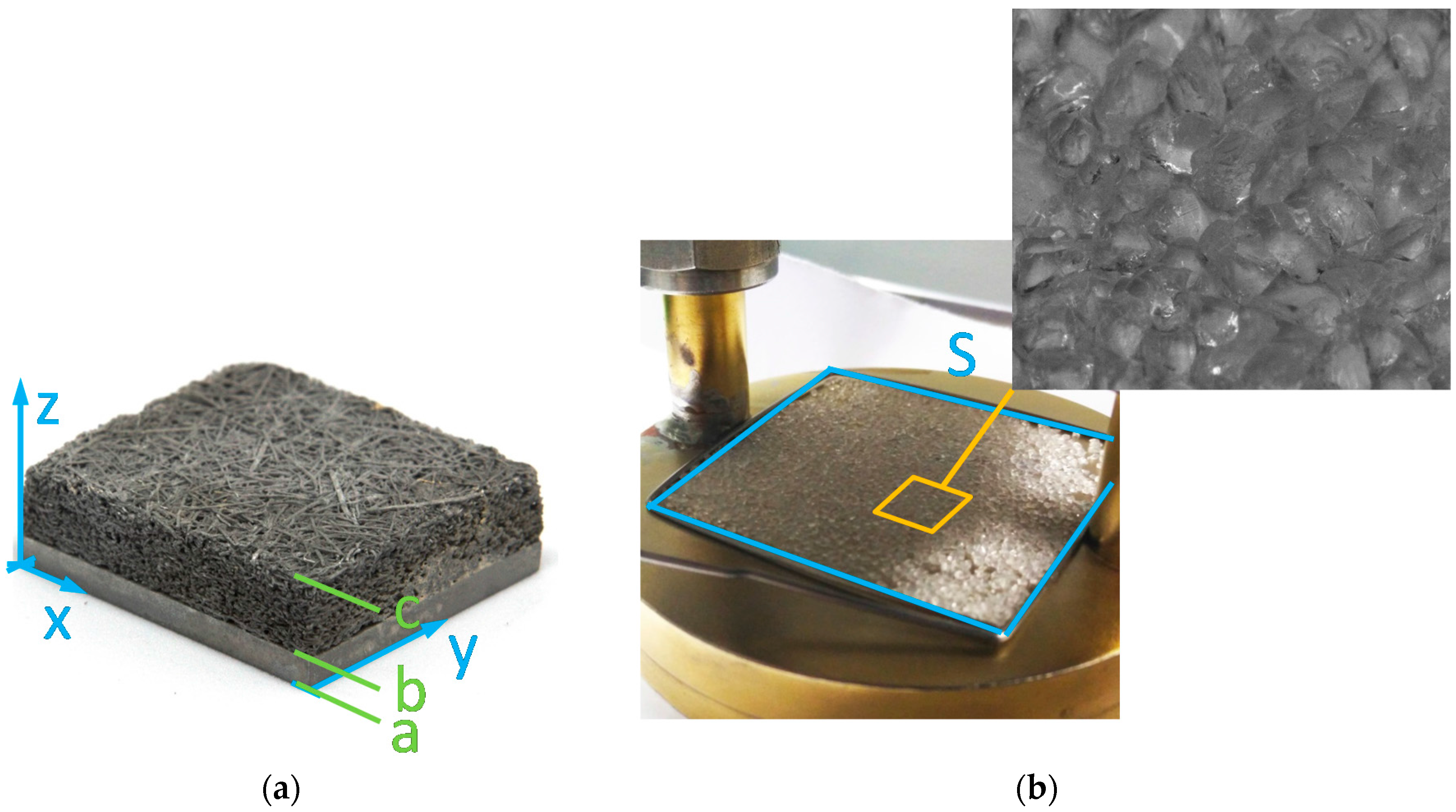
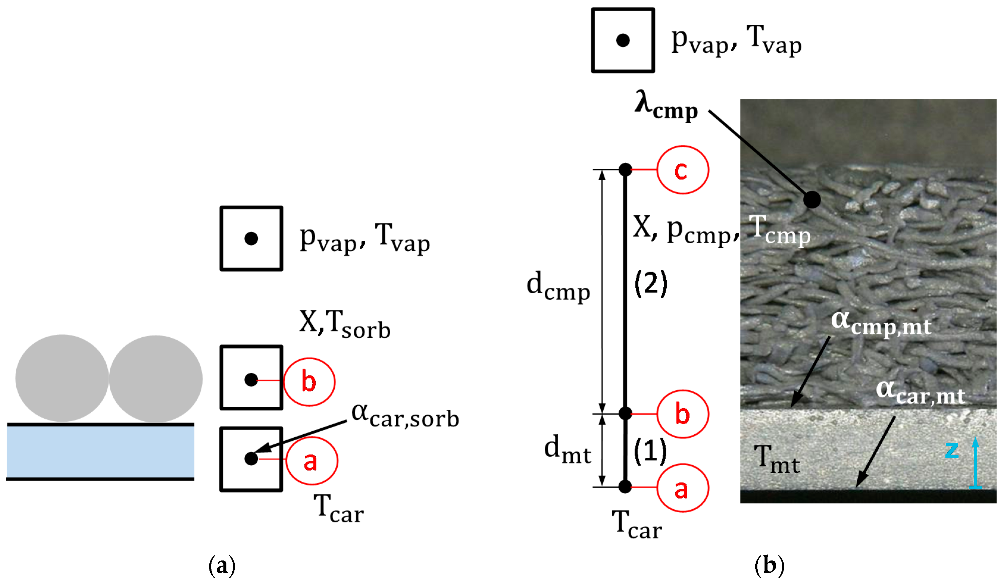
In order to demonstrate the applicability of the suggested measurement and simulation procedure, we present data for two completely different types of sorption samples, as shown in Figure 1 that reflect the wide range of different designs currently discussed in research. Additionally, a sample without adsorbent (flat plate, called ‘1_Plt’ in the following) was prepared. This sample is a flat aluminum plate, which is anodized. The black surface is best suited for the measurement with the infrared sensor since there are nearly no reflections. The thickness of the plate is 2 mm.

The data for a fibrous structures directly crystallized with SAPO-34 (fibrous structure called ‘2_Fib’ in the paper) as studied by Füldner [19], Füldner et al. [20], Wittstadt et al. [9] and Velte et al. [21] can be found in

Table 1. Data of the fibrous structure directly crystallized with SAPO-34 (2_Fib).

Description	Symbol	Unit	Value
Thickness of the metal sheet (distance a-b in Figure 1)	${\mathrm{d}}_{\mathrm{mt}}$	mm	2 ± 0.1
Thickness of the fibrous plate (distance b-c in Figure 1)	${\mathrm{d}}_{\mathrm{cmp}}$	mm	5 ± 0.1
Adsorbent mass (dry)	${\mathrm{M}}_{\mathrm{sorb}}$	g	1.18 ± 0.12
Ratio of adsorbent mass and volume of the fibrous structure	${\mathsf{\rho }}_{\mathrm{sorb},\mathrm{app}}$	kg/m³	522 ± 69
Ratio of fiber mass and volume of the fibrous structure	${\mathsf{\rho }}_{\mathrm{Fib},\mathrm{app}}$	kg/m³	588 ± 71
Mean macro pore diameter	${\mathrm{d}}_{\mathrm{maP}}$	µm	151 ± 20
Mean adsorbent layer thickness on the fibers	${\mathrm{d}}_{\mathrm{cryst}}$	µm	26 ± 3

. The directly-crystallized SAPO-34 has a chabazite (CHA) structure with a three-dimensional pore structure and a micro pore size of 3.8 Å [7]. More information about this adsorbent and the partial support transformation synthesis technique was published earlier by Bauer et al. [7]. The adsorbent mass as listed in Table 1 was determined by the manufacturer with measurements before and after the calcination. The mean macro pore diameter and the mean adsorbent layer thickness on the fibers are calculated quantities for an ideal cylindrical pore. Their uncertainties depend mainly on the uncertainty of the adsorbent mass. Füldner [19] also determined macro pore diameters of similar fibrous structures with permeability measurements. The results confirmed the validity of the geometrical model of the ideal cylindrical pores for the fibrous structures.

The data for a loose grains configuration of Siogel as studied by Sapienza et al. [22] (a silica gel from Oker-Chemie (Goslar, Germany), called ‘3_Sio’ in the paper) can be found in

Table 2. Data of the loose grains configuration of Siogel (3_Sio).

Description	Symbol	Unit	Value
Mean grain size	${\mathrm{d}}_{\mathrm{sorb}}$	mm	0.85–1
Adsorbent mass (dry)	${\mathrm{M}}_{\mathrm{sorb}}$	g	0.85 ± 0.05
Area as shown in Figure 1	$\mathrm{S}$	cm2	17.8 ± 21
Pore average diameter [22]	${\mathrm{d}}_{\mathrm{pore}}$	nm	2
Internal surface area [22]	${\mathrm{s}}_{\mathrm{int}}$	m2/g	800

. The grains are placed on the carrier plate directly in a monolayer configuration. The mean grain size interval is equivalent to the size of the sieve that was used to separate the grains. The adsorbent mass under atmospheric conditions (room temperature of 20 °C, relative humidity between 40% and 60%) was determined with a microbalance. The adsorbent dry mass was calculated using the equilibrium data of Siogel. The area S is the area on the carrier plate that is covered with the Siogel grains.

2.2. Modelling of Heat and Mass Transfer

The adsorption process is a strongly coupled heat and mass transfer process. A schematic drawing of the two samples studied here is shown in Figure 2.

2.2.1. General Mass Transfer Equations

In the most general formulation, Pentchev et al. [23] or more recently Leinekugel-le-coq et al. [24] describe the mass transfer of the adsorption process on three levels: the bulk (vapor) phase level, the macro pore (or pellet) level and the micro pore level. It is worth noting that not all types and shapes of adsorbent have to be described on the macro porous level and the micro porous level. In many cases, one of those levels can be neglected. However, in the future, we will present the equations in a rather general formulation and make simplifying assumptions for the different types and shapes of adsorbent studied here. On the vapor phase level, most authors use the law of the ideal gas to describe the dependency of pressure, temperature and vapor mass. The law of the ideal gas as shown in Equation (1) is valid for low pressures. This makes it best suited to the conditions of the adsorption processes with water vapor as a working fluid, since the pressure range for common temperature triples (desorption temperature, adsorption or condensing temperature, heat source or evaporation temperature) of many adsorbent-adsorbate pairs is well below the atmospheric pressure.

$${\mathrm{p}}_{\mathrm{vap}}\cdot {\mathrm{V}=\mathrm{M}}_{\mathrm{vap}}\cdot \frac{{\mathrm{R}}_{\mathrm{const}}}{{\mathrm{M}}_{\mathrm{mol},\mathrm{vap}}}\cdot {\mathrm{T}}_{\mathrm{vap}}$$

(1)

On the macropore level, we describe the mass transfer with the Fickian diffusion Equation (2); see Kast et al. [25] or Füldner [19]. The term on the left-hand side of Equation (2) is the time derivative of the gas phase concentration in the macro pores; the first term on the right-hand side is the diffusive transport. Furthermore, this equation includes a sink term ${\mathrm{J}}_{\mathrm{miP}}$, which accounts for the adsorption in the micro pores. This sink term has to be formulated depending on the geometrical resolution of the micro porous level and the macro porous level.

$$\frac{\partial {\mathrm{c}}_{\mathrm{maP}}}{\partial \mathrm{t}}=\nabla {\mathrm{D}}_{\mathrm{maP}}\nabla {\mathrm{c}}_{\mathrm{maP}} {-\mathrm{J}}_{\mathrm{miP}}$$

(2)

The adsorption on the micro porous level is also described with diffusion Equation (3) according to Füldner [19]. It is worth noting that the concentrations ${\mathrm{c}}_{\mathrm{maP}}$ and ${\mathrm{c}}_{\mathrm{miP}}$ refer to the vapour phase concentration of the adsorbate. The loading $\mathrm{X}$ can also be expressed in terms of the adsorbate concentration ${\mathrm{c}}_{\mathrm{adb}}$ as shown in Equation (4). The adsorbate concentration ${\mathrm{c}}_{\mathrm{adb}}$ is the concentration of the adsorbed phase. Thus, the diffusion coefficient ${\mathrm{D}}_{\mathrm{adb}}$ refers to the diffusion mechanism of the adsorbate that is already adsorbed in the micro pores of the adsorbent.

$$\frac{\partial {\mathrm{c}}_{\mathrm{miP}}}{\partial \mathrm{t}}=\nabla {\mathrm{D}}_{\mathrm{vap}}\nabla {\mathrm{c}}_{\mathrm{miP}}+\frac{{\mathsf{\varrho }}_{\mathrm{sorb}}}{{\mathsf{\psi }}_{\mathrm{cryst}}\cdot {\mathrm{M}}_{\mathrm{mol},\mathrm{vap}}}\cdot \nabla \left({\mathrm{D}}_{\mathrm{adb}}\cdot \frac{\mathrm{dlnp}}{\mathrm{dlnX}}\right)\nabla \mathrm{X}-\frac{{\mathsf{\rho }}_{\mathrm{sorb}}}{{\mathsf{\psi }}_{\mathrm{cryst}}\cdot {\mathrm{M}}_{\mathrm{mol},\mathrm{vap}}}\cdot \frac{\mathrm{dX}}{\mathrm{dt}}$$

(3)

$${\mathrm{X}=\mathrm{c}}_{\mathrm{adb}}\cdot \frac{{\mathsf{\psi }}_{\mathrm{cryst}}\cdot {\mathrm{M}}_{\mathrm{mol},\mathrm{vap}}}{{\mathsf{\varrho }}_{\mathrm{sorb}}}$$

(4)

The porosity of the crystallite (adsorbent) ${\mathsf{\psi }}_{\mathrm{cryst}}$ is a constant value as defined in Equation (5). The two densities ${\mathsf{\varrho }}_{\mathrm{cryst}}$ and ${\mathsf{\varrho }}_{\mathrm{sklt}}$ are the apparent density of the adsorbent including the pore volume (crystallite) and the pure material density of the adsorbent (skeleton density).

$${\mathsf{\psi }}_{\mathrm{cryst}}=\frac{{\mathsf{\varrho }}_{\mathrm{cryst}}}{{\mathsf{\varrho }}_{\mathrm{sklt}}}=\frac{{\mathrm{V}}_{\mathrm{sklt}}}{{\mathrm{V}}_{\mathrm{cryst}}}$$

(5)

In both diffusion Equations (2) and (3), it is necessary to define diffusion coefficients, which reflect the physics behind the mass transfer process. However, one has also to choose if both macro and micro porous diffusion have to be modelled or if one of those levels can be neglected. Here, we present experimental data for a layer of loose silica gel grains and a fibrous structure with a directly crystallized layer of SAPO-34. The general form of the mass and heat transfer model is adapted to the specifics of the two differing types of samples.

2.2.2. Linear Driving Force Approach

If the diffusion in the adsorbed phase dominates, Equation (3) can be simplified as shown in Equation (6) [19]. In Equation (6), the driving potential of the mass transfer is the loading $\mathrm{X}$

$$\frac{\mathrm{dX}}{\mathrm{dt}}=\nabla \left({\mathrm{D}}_{\mathrm{adb}}\cdot \frac{\mathrm{dlnp}}{\mathrm{dlnX}}\right)\nabla \mathrm{X}\cdot$$

(6)

Even if the diffusion in the adsorbed phase will dominate, the diffusion coefficient ${\mathrm{D}}_{\mathrm{adb}}$ might not be constant. It is likely that it depends on the loading and also the temperature of the adsorbent. In order to discover the loading dependency of ${\mathrm{D}}_{\mathrm{adb}}$, Füldner [19] performed differential pressure step measurements on SAPO-34. The evaluation of these measurements with an analytical diffusion model revealed that this coefficient only slightly depends on the loading. Since the observed differences were within the measurement errors, a constant diffusion coefficient seems to be justified. More recently, Stallmach et al. [26] have shown with pulsed field gradient nuclear magnetic resonance (PFG-NMR) measurements that the diffusion coefficient does not depend much on the loading, but on the temperature. However, the influence of the temperature is small compared to measurement errors. Thus, the choice of a constant diffusion coefficient in case of SAPO-34 seems justified.

Under the following assumptions, the spatially-distributed Equation (6) can be simplified to the linear driving force (LDF) approach as shown in Equation (7) [19].

• Linear sorption isotherm $\frac{\mathrm{d}\ln \mathrm{p}}{\mathrm{d}\ln \mathrm{X}}=1$
• Parabolic loading profile in the adsorbent layer or particle:

  $$\frac{\mathrm{d}\overline{\mathrm{X}}}{\mathrm{dt}}={\mathrm{k}}_{\mathrm{LDF}}·({\mathrm{X}}_{\mathrm{eqi}}-\overline{\mathrm{X}}).$$

  (7)

The overbar symbol denotes that the loading $\overline{\mathrm{X}}$ is a spatially-averaged quantity.

2.2.3. Mass Transfer Model for the Loose Grains Configuration

First, we focus on the mass transfer model for the layer of loose silica gel grains. In the case of a monolayer of silica gel, the macro porous level can be neglected because the average pore diameter in the grain is in the range of $2–15 \mathrm{nm}$ for micro and meso porous silica gel types [3], and the vapor pressure around a single grain is nearly uniform. This assumption holds true for a monolayer configuration, since each grain is in direct contact with the vapor volume. If a multilayer configuration is modelled, the vapor transport through the adsorbent bed would have to be considered.

In Equation (3), we can distinguish between two extreme cases. When diffusion in the gas phase dominates the adsorption process, Equation (3) can be simplified to Equation (8). As can be seen in Equation (8), the effective diffusion coefficient for the micro porous mass transfer is the diffusion coefficient in the gas phase.

$$\frac{\partial {\mathrm{c}}_{\mathrm{miP}}}{\partial \mathrm{t}}=\nabla {\mathrm{D}}_{\mathrm{vap}}\nabla {\mathrm{c}}_{\mathrm{miP}}-\frac{{\mathsf{\varrho }}_{\mathrm{sorb}}}{{\mathsf{\psi }}_{\mathrm{cryst}}\cdot {\mathrm{M}}_{\mathrm{mol},\mathrm{vap}}}\cdot \frac{\mathrm{dX}}{\mathrm{dt}}$$

(8)

A similar formulation is used by Freni et al. [27] in a simulative study of a loose grains configuration of silica gel with a constant value of ${\mathrm{D}}_{\mathrm{miP}}{=4\times 10}^{-7} {\mathrm{m}}^2/\mathrm{s}$. Furthermore, Okunev et al. [28,29] use the formulation in Equation (8) in a simulative and experimental study of the water adsorption of a loose grains configuration of a selective water adsorbent (SWS-1L).

However, if one assumes diffusion in the adsorbed phase for the Siogel grains, the LDF approach in Equation (7) can be used as a simplified mass transfer model. In this case, the two- or three-dimensional diffusion problem of Equation (8) is reduced to a zero-dimensional LDF equation with a single value for the spatially-averaged loading $\overline{\mathrm{X}}$, as shown in Figure 2. Recently, this formulation was used by Graf et al. [16] in their simulation of a silica gel adsorber. Furthermore, the models of air-to-air heat wheels with silica gel of Fathieh et al. [30,31] are based on the assumptions of the LDF approach. This results in an LDF formulation for the temperature response of the heat wheel [30] or a double exponential model for the humidity response of the heat wheel [31]. Due to its simplicity, we use this approach in the following paper, although the assumption of the diffusion in the adsorbed phase might not be correct. The equilibrium loading ${\mathrm{X}}_{\mathrm{eqi}}$ is calculated from vapor pressure ${\mathrm{p}}_{\mathrm{vap}}$ and adsorbent temperature ${\mathrm{T}}_{\mathrm{sorb}}$. For the equilibrium description ${\mathrm{X}}_{\mathrm{eqi}}\left(\mathrm{p},\mathrm{T}\right)$ of Siogel, we use the Dubinin-Astakhov equation published by Sapienza et al. [22].

2.2.4. Mass Transfer Model for the Fibrous Structure

The macro pore level of the fibrous structure is modelled with the one-dimensional diffusion Equation (2). The sink term in this equation depends on the local change in loading, the macro porosity of the composite ${\mathsf{\psi }}_{\mathrm{cmp}}$, the mass fraction of adsorbent ${\mathsf{\zeta }}_{\mathrm{sorb}}$ and the apparent density of the composite ${\varrho }_{\mathrm{cmp},\mathrm{app}}$.

$${\mathrm{J}}_{\mathrm{miP}}=- \frac{\mathrm{dX}}{\mathrm{dt}}\cdot \frac{{\mathsf{\zeta }}_{\mathrm{sorb}}\cdot {\mathsf{\varrho }}_{\mathrm{cmp},\mathrm{app}}}{{\mathrm{M}}_{\mathrm{mol},\mathrm{vap}}\cdot {\mathsf{\psi }}_{\mathrm{cmp}}}$$

(9)

The diffusion coefficient for the macro pore level ${\mathrm{D}}_{\mathrm{maP}}$ is a combination of Knudsen diffusion and viscous flow in a cylindrical pore [19,21]. For the diffusion on the micro pore level, the spatially-distributed Equation (6) can be used, since the diffusion in the adsorbed phase will dominate in the case of the compact SAPO-34 layer (the crystallite layer thickness of the directly-crystallized layer is ${\mathrm{d}}_{\mathrm{cryst}} \approx 20 \mu \mathrm{m}–40 \mu \mathrm{m}$). When it comes to simulations on the heat exchanger level or the module level including a dynamic model of the condenser and evaporator, solving the diffusion Equation (3) on the micro pore level can be computationally too expensive. In this case, the LDF approach according to Equation (7) can be used to create a simplified model. Our aim is to identify the parameters for a model that is suited for simulations on the heat exchanger or the module level. Thus, we focus here on the LDF approach according to Equation (7), although the assumption of a linear sorption isotherm is not fulfilled in the case of SAPO-34. The equilibrium loading ${\mathrm{X}}_{\mathrm{eqi}}$ is calculated with the pressure in the macro pores ${\mathrm{p}}_{\mathrm{maP}}$ and the temperature of the composite ${\mathrm{T}}_{\mathrm{cmp}}$. It has to be noted that the equilibrium loading ${\mathrm{X}}_{\mathrm{eqi}}$ and the loading $\overline{\mathrm{X}}$ are spatially distributed quantities along the one-dimensional domain (z-axis), as shown in Figure 2 in this case. The spatial average of the loading $\overline{\mathrm{X}}$ refers to the average over the crystallite layer thickness, which is not modelled as a separate domain. For the directly-crystallized SAPO-34, an equilibrium description ${\mathrm{X}}_{\mathrm{eqi}} \left(\mathrm{p},\mathrm{T}\right)$ according to the generalized statistical thermodynamic adsorption model of Llano-Restrepo et al. [32] is used. The directly-crystallized SAPO-34 is similar to the adsorbent FAM-Z02 as studied by Girnik et al. [13].

2.2.5. Heat Transfer Model for the Loose Grains Configuration

Since the LDF approach is used for the mass transfer model and the macro pore diffusion is neglected, the grain is reduced to a single point (b). This point has the two state variables loading $\mathrm{X}$ and temperature ${\mathrm{T}}_{\mathrm{sorb}}$. The adsorbent temperature ${\mathrm{T}}_{\mathrm{sorb}}$ is calculated using the energy balance in Equation (10). The temperature of the carrier plate is ${\mathrm{T}}_{\mathrm{car}}$. The adsorption enthalpy ${\mathrm{h}}_{\mathrm{ads}}$ is calculated out of the adsorption potential $\mathrm{A}\left({\mathrm{p}}_{\mathrm{vap}}{,\mathrm{T}}_{\mathrm{sorb}}\right)$ using the equilibrium description of Siogel and the enthalpy difference between liquid water and water vapor ${\mathsf{\Delta }\mathrm{h}}_{\mathrm{lv}}\left({\mathrm{T}}_{\mathrm{sorb}}\right)$ according to Equation (11). The adsorption potential is defined in Equation (12). The enthalpy of the vapor from the gas phase ${\mathrm{h}}_{\mathrm{vap}}$ is calculated with the state variables of the gas phase and the adsorbent temperature. For the studied boundary conditions, the adsorption enthalpy is within a range of $2650–2800 \mathrm{kJ}/\mathrm{kg}$ for adsorption and $2500–2750 \mathrm{kJ}/\mathrm{kg}$ for desorption, respectively. The heat transfer resistance caused by the finite heat conductivity within the grain is neglected, since it is assumed to be sufficiently smaller than the heat transfer resistance between the grain and carrier plate. For the mean grain size studied here and the heat conductivity given by Freni et al. [27], this is the case, since $\mathrm{Bi}={\mathsf{\alpha }}_{\mathrm{car},\mathrm{sorb}}\cdot {\mathrm{d}}_{\mathrm{sorb}}/\left(2\cdot {\mathsf{\lambda }}_{\mathrm{sorb}}\right)\approx 0.1$. However, if a bigger grain size is modelled, this resistance has to be taken into account.

$$\left({\mathrm{M}}_{\mathrm{sorb}}\cdot {\mathrm{c}}_{\mathrm{p}.\mathrm{sorb}} + \mathrm{X}\cdot {\mathrm{M}}_{\mathrm{sorb}}\cdot {\mathrm{c}}_{\mathrm{p},\mathrm{liq}}\left({\mathrm{T}}_{\mathrm{sorb}}\right)\right)\cdot \frac{{\mathrm{dT}}_{\mathrm{sorb}}}{\mathrm{dt}}{=\mathrm{M}}_{\mathrm{sorb}}\cdot \frac{\mathrm{dX}}{\mathrm{dt}}\cdot {\mathrm{h}}_{\mathrm{ads}}{ + \mathrm{M}}_{\mathrm{sorb}}\cdot \frac{\mathrm{dX}}{\mathrm{dt}}\cdot {\mathrm{h}}_{\mathrm{vap}}{-\mathsf{\alpha }}_{\mathrm{car},\mathrm{sorb}}\cdot \mathrm{S}\cdot \left({\mathrm{T}}_{\mathrm{sorb}}{-\mathrm{T}}_{\mathrm{car}}\right)$$

(10)

$${\mathrm{h}}_{\mathrm{ads}}{=\mathsf{\Delta }\mathrm{h}}_{\mathrm{lv}}\left({\mathrm{T}}_{\mathrm{sorb}}\right) + \mathrm{A}\left({\mathrm{p}}_{\mathrm{vap}}{,\mathrm{T}}_{\mathrm{sorb}}\right)$$

(11)

$$\mathrm{A}\left({\mathrm{p}}_{\mathrm{vap}}{,\mathrm{T}}_{\mathrm{sorb}}\right)=\frac{{\mathrm{R}}_{\mathrm{const}}\cdot {\mathrm{T}}_{\mathrm{sorb}}}{{\mathrm{M}}_{\mathrm{mol},\mathrm{vap}}}\cdot \ln \left(\frac{{\mathrm{p}}_{\mathrm{sat}}\left({\mathrm{T}}_{\mathrm{sorb}}\right)}{{\mathrm{p}}_{\mathrm{vap}}}\right)$$

(12)

2.2.6. Heat Transfer Model for the Fibrous Structure

The temperature of the composite $T_{cmp}$ is calculated with the energy balance in Equation (13). The loading-dependent heat capacity of the composite ${\mathrm{c}}_{\mathrm{p},\mathrm{cmp}}\left(\mathrm{X}\right)$ as shown in Equation (14) takes into account the heat capacity of the aluminum fibers, the dry adsorbent and the adsorbed water.

$$\frac{\left({\mathrm{M}}_{\mathrm{sorb}}{ + \mathrm{M}}_{\mathrm{Fib}}\right)}{{\mathrm{V}}_{\mathrm{cmp}}}\cdot {\mathrm{c}}_{\mathrm{p},\mathrm{cmp}}\left(\mathrm{X}\right)\cdot \frac{\partial {\mathrm{T}}_{\mathrm{cmp}}}{\partial \mathrm{t}}=\nabla \cdot \left({\mathsf{\lambda }}_{\mathrm{cmp}}{\mathrm{T}}_{\mathrm{cmp}}\right) + \frac{\partial \mathrm{X}}{\partial \mathrm{t}}\cdot {\mathrm{h}}_{\mathrm{ads}}\cdot {\mathsf{\varrho }}_{\mathrm{sorb}}$$

(13)

$${\mathrm{c}}_{\mathrm{p},\mathrm{cmp}}\left(\mathrm{X}\right)=\frac{{\mathrm{M}}_{\mathrm{sorb}}}{{\mathrm{M}}_{\mathrm{cmp}}}\cdot \left({\mathrm{c}}_{\mathrm{p},\mathrm{sorb}} + \mathrm{X}\cdot {\mathrm{c}}_{\mathrm{p},\mathrm{adb}}\right) + \frac{{\mathrm{M}}_{\mathrm{Fib}}}{{\mathrm{M}}_{\mathrm{cmp}}}\cdot {\mathrm{c}}_{\mathrm{p},\mathrm{Fib}}$$

(14)

The heat capacity of the aluminum fibers is $900 \mathrm{J}/\mathrm{kg}$. The heat capacity of the adsorbent, which is SAPO-34 in this case, is assumed to be 900 J/kg. This value was not measured by the authors. It is an assumption based on the fact that the adsorbent crystals grow on the aluminum surface, and aluminum is part of the adsorbent crystals [7]. The heat conductivity of the composite material ${\mathsf{\lambda }}_{\mathrm{cmp}}$ is not known. As explained later in Section 3.2, a good upper bound for this parameter is the measured heat conductivity of the uncoated fibrous structure. Since this parameter is very important for the overall dynamics, we chose to vary it in the model calibration procedure. Moreover, the heat conductivity of the adsorbent layer will change with the loading. This change is neglected in the overall heat conductivity ${\mathsf{\lambda }}_{\mathrm{cmp}}$ of the composite. Since the mean adsorbent layer thickness is thin (26 µm), the heat transfer resistance within the adsorbent layer caused by the heat conductivity of the adsorbent is neglected.

Due to the more complex equilibrium description in the case of SAPO-34, we assume a constant value for the adsorption enthalpy ${\mathrm{h}}_{\mathrm{ads}}=3200 \mathrm{kJ}/\mathrm{kg}$. This approach is commonly used in combination with Equation (15) for the heat capacity of the adsorbate. To the knowledge of the authors, independent measurements for the adsorption enthalpy have not been published yet.

$${\mathrm{c}}_{\mathrm{p},\mathrm{adb}}\left(\mathrm{T}\right){=\mathrm{c}}_{\mathrm{p},\mathrm{vap}}\left(\mathrm{T}\right)$$

(15)

The heat transfer in the metal domain (1) is described with a heat conduction equation with the state variable ${\mathrm{T}}_{\mathrm{mt}}$. At Boundary c, the enthalpy of the incoming water vapor during adsorption is taken into account. The metal plate (1) and composite (2) are connected via the boundary condition in Equation (16), taking into account a contact resistance between them.

$$\stackrel{·}{\mathrm{q}}{|}_{\mathrm{b}}={\mathsf{\alpha }}_{\mathrm{cmp},\mathrm{mt}}·({\mathrm{T}}_{\mathrm{mt}}-{\mathrm{T}}_{\mathrm{cmp}})$$

(16)

Between the metal plate (1) and the carrier plate, another contact resistance is taken into account according to Equation (17).

$$\stackrel{·}{\mathrm{q}}{|}_{\mathrm{a}}={\mathsf{\alpha }}_{\mathrm{car},\mathrm{mt}}·({\mathrm{T}}_{\mathrm{car}}-{\mathrm{T}}_{\mathrm{mt}})$$

(17)

The surface temperature is the composite temperature at Point c. Here, a source term for the enthalpy of the vapor from the gas phase is set during adsorption (heat up or cool down the incoming vapor).

2.3. Experimental Setup and Measurement Procedure

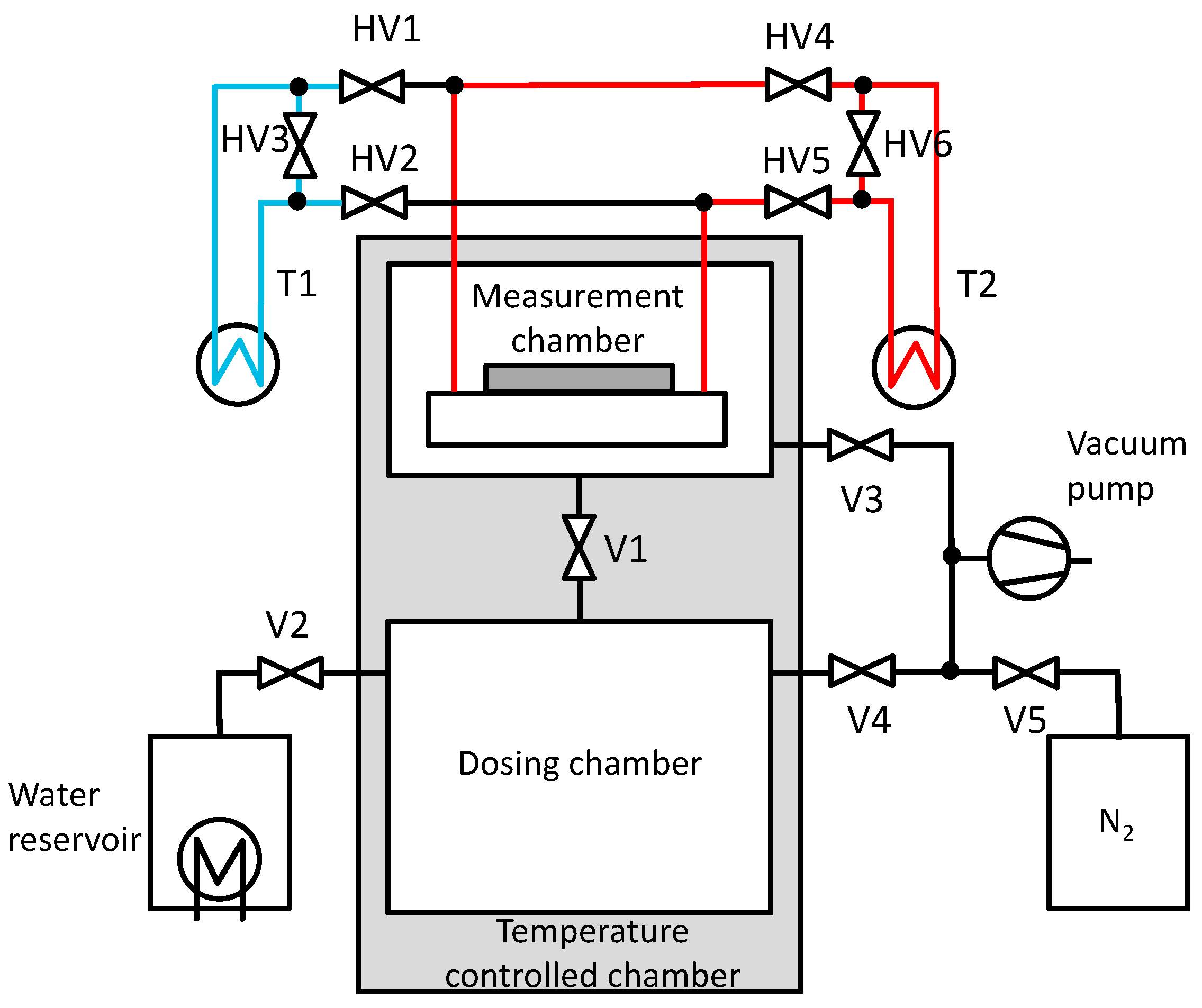
Figure 3 shows a schematic drawing of the recently-modified kinetic setup at Fraunhofer ISE in which both large pressure jump measurements (LPJ) as described by Schnabel et al. [8] and Füldner et al. [19], as well as large temperature jump measurements (LTJ) as described by Aristov et al. [15] can be performed. A brief description of the current setup was given earlier [22]. The basis for the setup was described first by Schnabel [18] and Schnabel et al. [8]. The recent modification is the connection of a nitrogen dosage unit. If both the measurement chamber and the dosing chamber are evacuated, the vacuum pump is switched off. Then, both chambers can be filled with dry nitrogen by opening of the valves V3, V4 and V5. The pressure in the measurement chamber and the dosing chamber is measured with two separate pressure sensors (Baratron 627B (MKS Instruments, Andover, MA, USA)). The surface temperature of the sample placed in the measurement chamber is measured with an infrared sensor (Optris CT Fast (Optris, Berlin, Germany)). In order to indicate the measurement of the surface temperature with the infrared sensor, we call the measurements IR-LPJ and IR-LTJ in the following. The temperature of the thermostats T1 and T2 is measured with Pt-100 sensors. Furthermore, the vapor temperature in the dosing chamber is measured with two Pt-100 sensors. As a prerequisite for each measurement, the measurement chamber with the sample inside is fully evacuated. The carrier plate is heated to a maximum value of 95 °C while the vacuum pump stays connected to the measurement chamber. These conditions are kept over 4 h to make sure that all water vapor or gas is desorbed from the sample.

With the nitrogen dosage unit as described above, also another kind of measurement can be performed. Nitrogen can be regarded as an inert species for the adsorbents and the conditions studied here. As soon as a nitrogen pressure in the range of 0.1–100 mbar is set, the adsorbent will neither ad- or de-sorb nitrogen, although the temperature of the sample is changed in the range of 30 °C and 95 °C. Thus, the measurement is isosterical, and hence, there will be no release of the heat of adsorption. The measurement procedure is continued by connecting the carrier plate to the thermostat T1 (low temperature). Then, the hydraulic valves are switched and the carrier plate is connected to the thermostat T2 (high temperature). In such an inert large temperature jump (inert-LTJ) measurement, the nitrogen pressure is set to the value of the water vapor pressure of the LTJ experiment. In such measurements, only the heat capacity of the sample, the thermal conductivity of the sample and the thermal coupling between the sample and the carrier plate influence the temperature change of the sample. The time-dependent surface temperature change of the sample can be measured with the infrared sensor and can be used as a signal for parameter identification with an appropriate numerical heat transfer model. Especially in the case of a loose grains configuration, it can be expected that the heat transfer processes between the grain and the carrier plate strongly depend on the presence of a vapor or a gas phase, since the direct contact area is very small compared to the maximum cross-sectional area of a grain [33]. If the chambers are evacuated to a pressure below 0.01 mbar, the only heat transfer process in the absence of the vapor or gas phase is the radiative heat transfer between the grain and carrier plate. However, nitrogen and water vapor do have different thermo-physical properties. It has to be carefully discussed to what extent the identified heat transfer parameters of an inert-LTJ measurement can be directly related to the parameters obtained from LTJ or LPJ experiments. 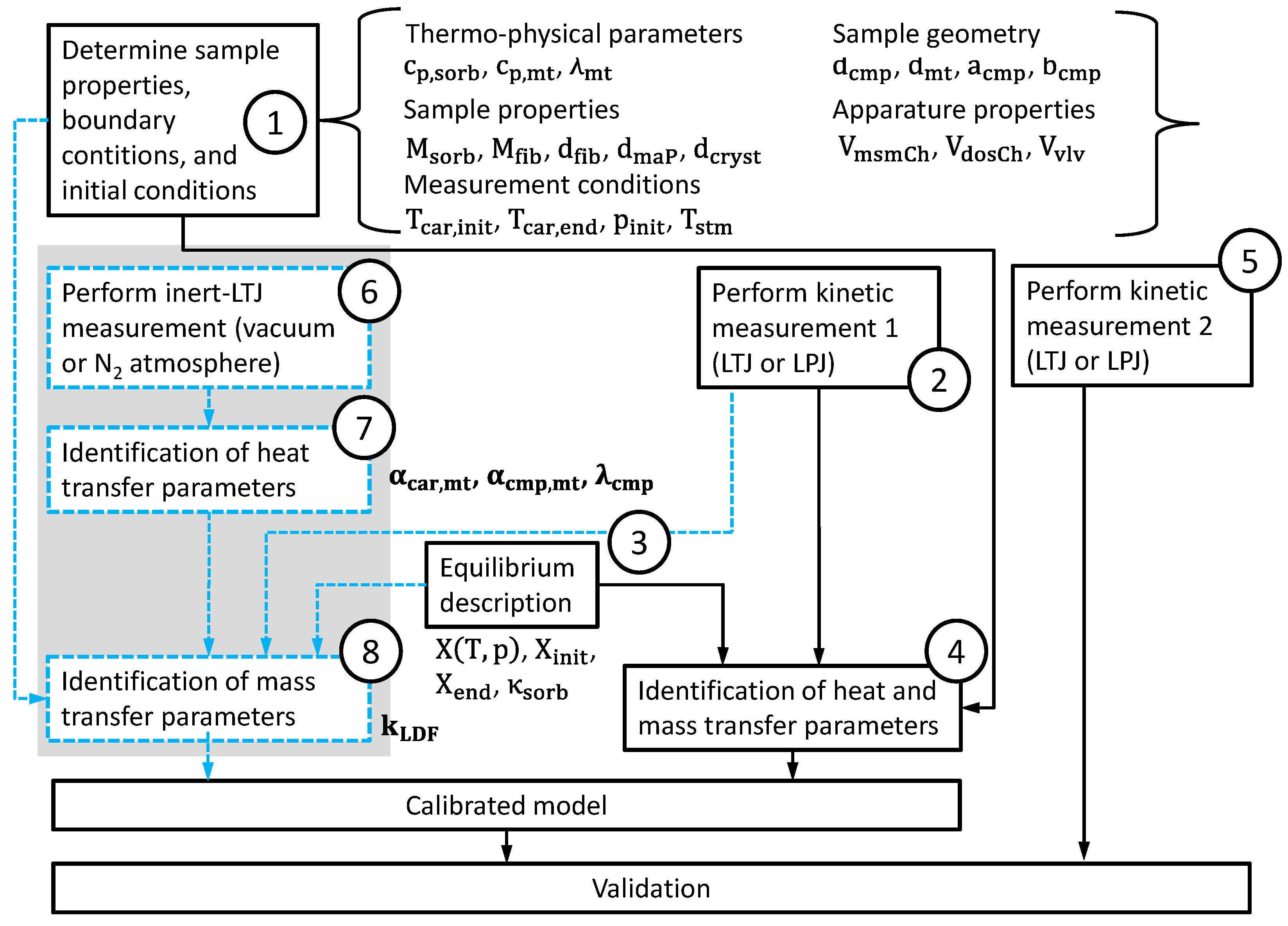Figure 4 shows the suggested measurement and simulation procedure with the additional inert-LTJ measurements. In the first step (1), all known sample parameters and aperture parameters, as well as the boundary conditions and the initial conditions are collected or defined. Then, the measurement procedure starts. The well-known part of the procedure is the kinetic experiment and the identification of heat and mass transfer parameters (Steps 2, 3 and 4). As soon as the equilibrium description is defined (Step 3), the equilibrium loading at the beginning ${\mathrm{X}}_{\mathrm{init},\mathrm{eqi}}$ and ${\mathrm{X}}_{\mathrm{end},\mathrm{eqi}}$ can be calculated with the initial and end values for pressure and sample temperature. Due to the measurement errors in pressure and temperature, the uncertainty in the determination of the mass of the adsorbent and differences between the equilibrium description and the actual behavior of the adsorbent, the measured uptake ${\mathsf{\Delta }\mathrm{X}}_{\mathrm{xpr}}$ might differ from the calculated uptake ${\mathsf{\Delta }\mathrm{X}}_{\mathrm{eqi}}$. A measure for this difference is the ratio ${\mathsf{\kappa }}_{\mathrm{sorb}}$ as defined in Equation (18). This ratio is used in the simulation to calibrate the simulated uptake in order to achieve the experimental end pressure without adapting any other parameters.

$${\mathsf{\kappa }}_{\mathrm{sorb}}=\frac{{\mathsf{\Delta }\mathrm{X}}_{\mathrm{xpr}}}{{\mathsf{\Delta }\mathrm{X}}_{\mathrm{eqi}}}=\frac{{\mathsf{\Delta }\mathrm{X}}_{\mathrm{xpr}}}{{\mathrm{X}}_{\mathrm{end},\mathrm{eqi}}{-\mathrm{X}}_{\mathrm{init},\mathrm{eqi}}}$$

(18)

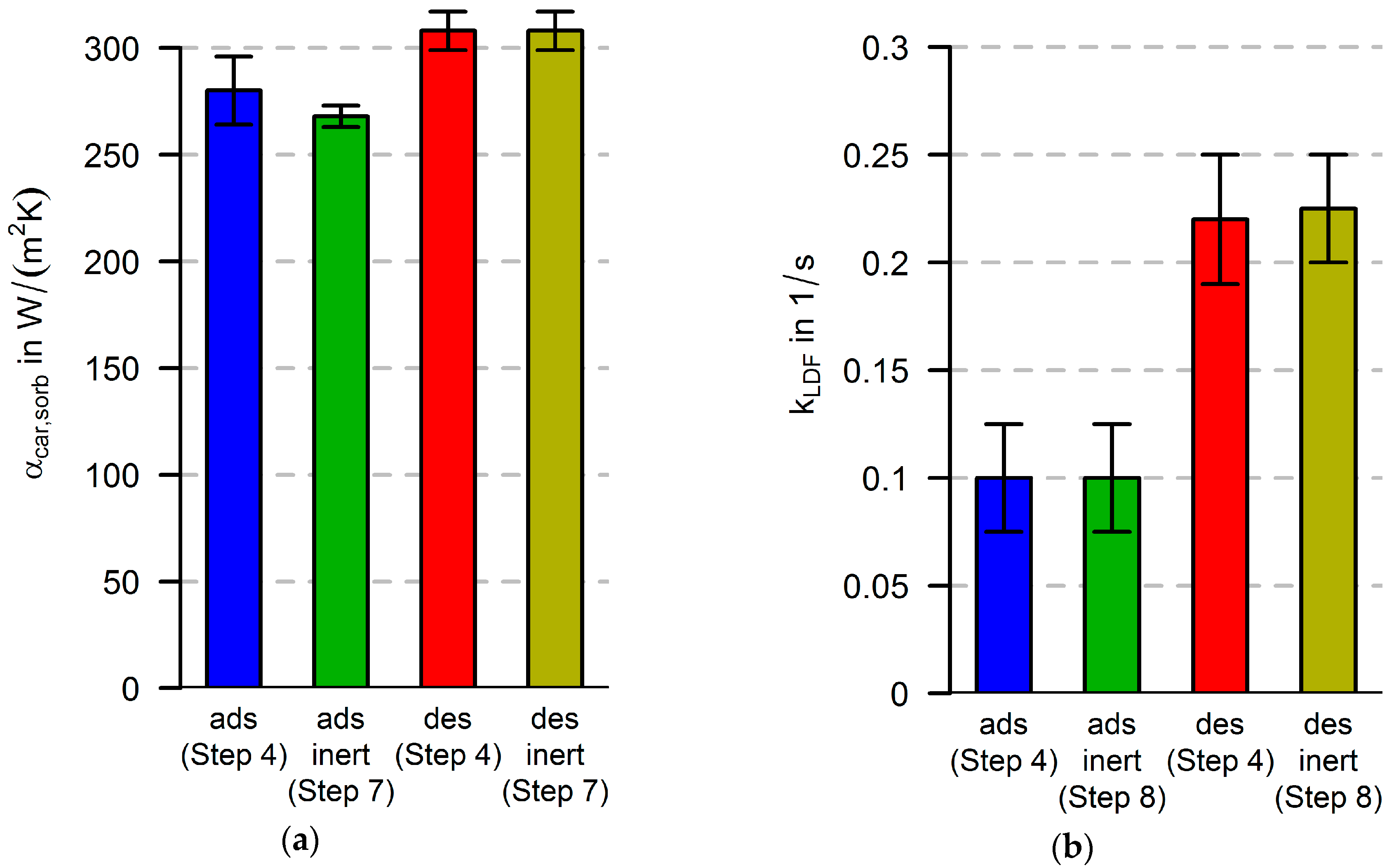
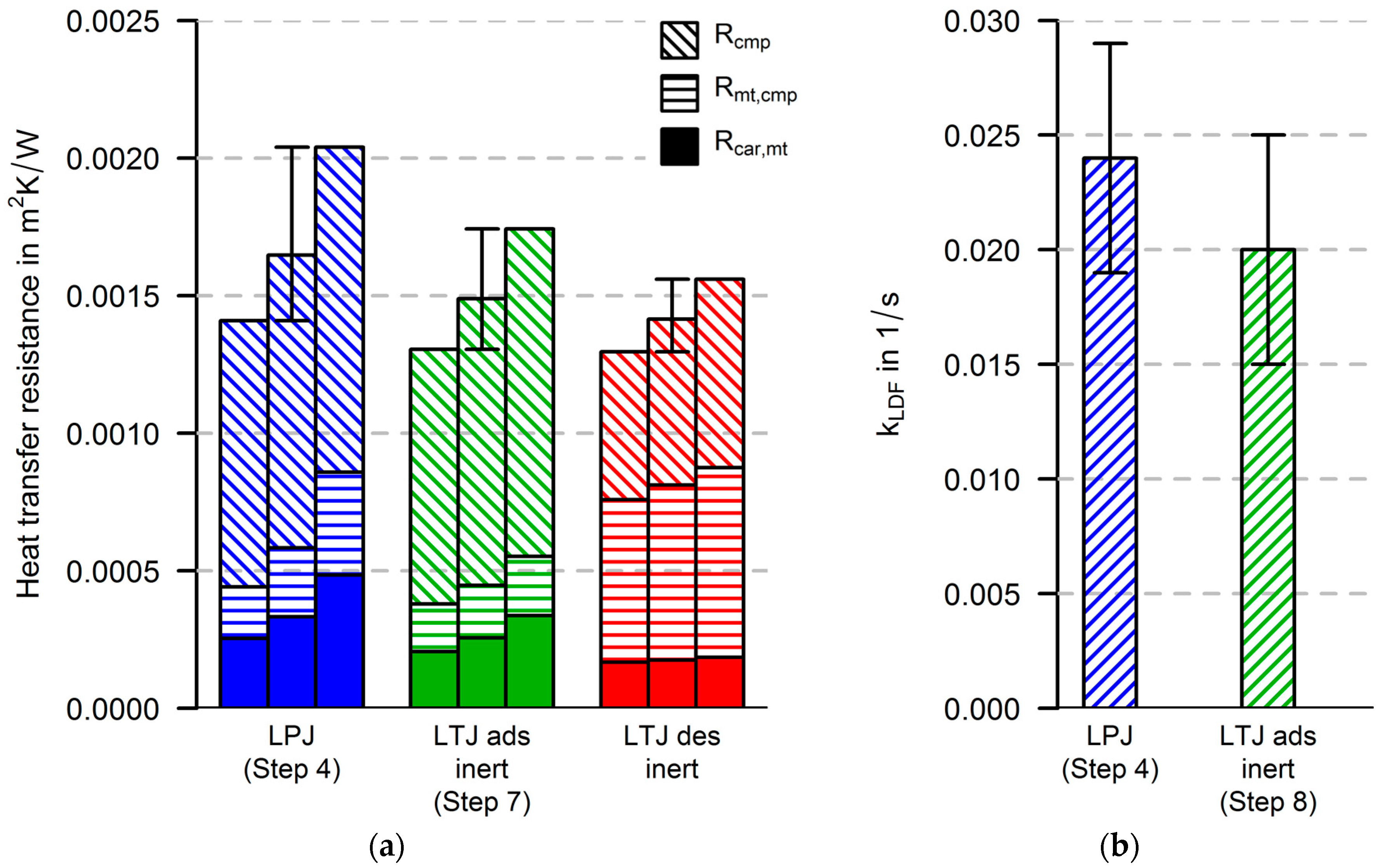
For the new measurement and simulation procedure, three more steps (6, 7 and 8) are suggested in order to separate the identification of heat transfer parameters from the identification of mass transfer parameters. The heat transfer parameters are identified by fitting simulation data to the experimental data of an inert-LTJ experiment (Step 6). This kind of experiment can be compared to flash analysis as first presented by Parker et al. [34] or other methods that are suited to determine heat transfer parameters. It is worth noting that also in the field of air-to-air energy wheels that are used for air dehumidification, kinetic measurements (temperature jumps or humidity jumps) are performed in order to determine model parameters [30,31]. Here, it could also be an option to perform inert temperature jumps in order to study only the heat transfer characteristics without the influence of the adsorption material.

In this paper, both procedures are performed, and the parameters from both procedures are evaluated. Thus, two parameter sets for heat and mass transfer parameters are obtained. If there are strong differences in the parameter sets, they will have to be discussed. This can be an indicator that improvements have to be made in at least one of the following model parts: the heat transfer part (e.g., heat capacities, spatial resolution), the equilibrium description of the adsorbent and the model for the calculation of the adsorption enthalpy.

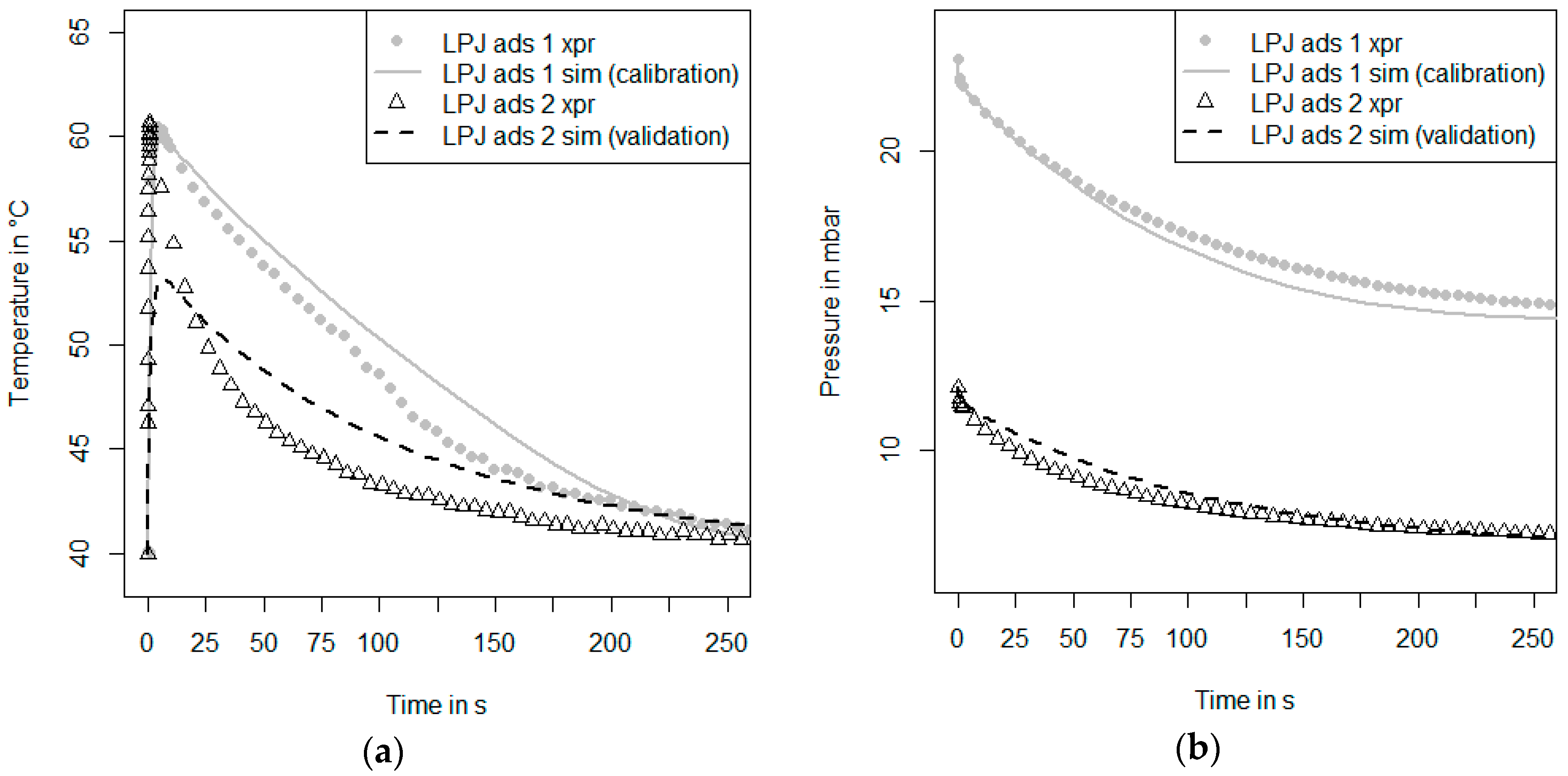
As soon as we have a well-calibrated model that is able to describe both the inert LTJ and the first kinetic experiment, a second kinetic measurement under different initial conditions can be evaluated. This is the validation Step 5 in Figure 4.

The initial conditions are listed in

Table 3. Measurement initial conditions. LPJ, large pressure jump.

Sample	Measurement	#	Carrier Plate Temperature in °C		Initial Pressure in mbar
			init	end	msmCh	dosCh
1_Plt	inert-LTJ adsorption	1	60	30	vacuum	-
1_Plt	inert-LTJ desorption	2	60	90	vacuum	-
2_Fib	inert-LTJ adsorption	3	64.5	30	vacuum	-
2_Fib	inert-LTJ desorption	4	58.5	90	vacuum	-
2_Fib	LPJ Adsorption 1	5	40		3.90	23.07
2_Fib	LPJ Adsorption 2	6	40		1.00	12.11
3_Sio	inert-LTJ adsorption	7	55.5	30	12.01
3_Sio	inert-LTJ desorption	8	51.5	80	41.90
3_Sio	LTJ adsorption	9	55.5	30	12.04
3_Sio	LTJ desorption	10	51.5	80	41.73
3_Sio	LPJ adsorption	11	30		0.62	12.05

for all measurements. For IR-LPJ measurements, the carrier plate temperature is not varied during the measurement. In the case of IR-LTJ measurements, the initial pressure in the measurement chamber is the same as in the dosage chamber, since both chambers are connected throughout the measurement. The initial and end temperatures of the IR-LTJ measurements and the inert-LTJ measurements are chosen according to the typical temperature conditions of a heat pump or a chiller that can be addressed with the material. Since SAPO-34 and Siogel have different adsorption equilibria, the temperatures differ.

2.4. Model Calibration and Validation

Depending on sample and type of the measurement, different models that reflect the different boundary conditions and physics behind the measurement were developed. In

Table 4. Model overview. LDF, linear driving force.

Model Name	Sample	Measurement	Physics
1_Plt_inertLTJ	1_Plt	inert-LTJ	Energy balance similar to Equation (13) without the source term for adsorptive heat, 1D spatial resolution along the z-axis, LTJ boundary and initial conditions
2_Fib_inertLTJ	2_Fib	inert-LTJ	Energy balance similar to Equation (13) without the source term for adsorptive heat, 1D spatial resolution along the z-axis, LTJ boundary and initial conditions
3_Sio_inertLTJ	3_Sio	inert-LTJ	Energy balance similar to Equation (10) without the source term for adsorptive heat and vapor enthalpy term, no spatial resolution, LTJ boundary and initial conditions
2_Fib_LPJ	2_Fib	LPJ	Energy balance Equation (13), mass transfer in the macro pores according to Equations (2) and (9), both 1D spatial resolution along the z-axis, LDF approach according to Equation (7) for micro pore diffusion, LPJ boundary and initial conditions
3_Sio_LTJ	3_Sio	LTJ	Energy balance Equation (10), LDF approach according to Equation (7), no spatial resolution, LTJ boundary and initial conditions
3_Sio_LPJ	3_Sio	LPJ	Energy balance Equation (10), LDF approach according to Equation (7), no spatial resolution, LPJ boundary and initial conditions

, an overview is given.

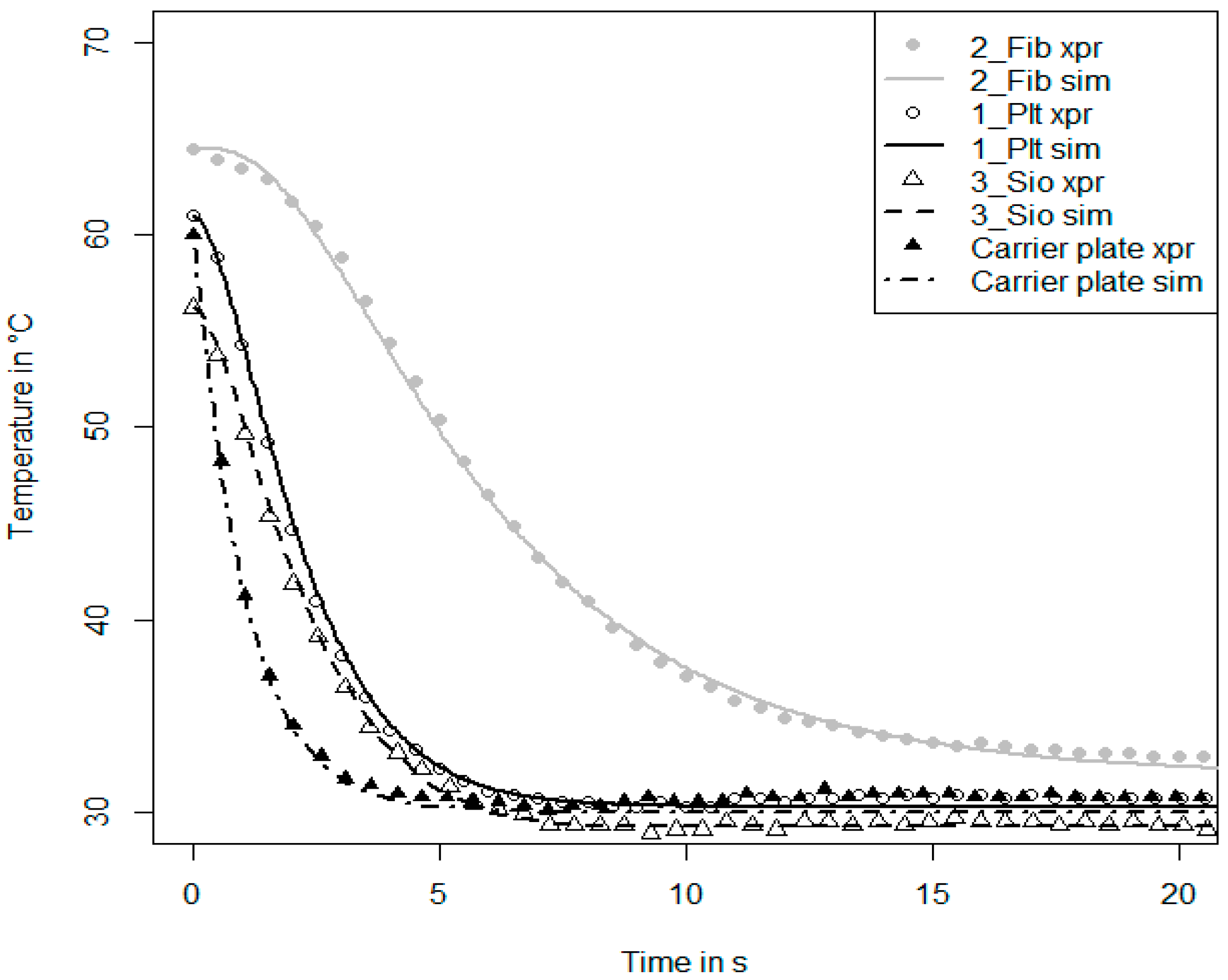
In the case of the inert-LTJ measurements, we use the surface temperature signal for the calibration procedure. For the IR-LPJ and IR-LTJ measurements, we use both the surface temperature signal and the pressure signal. For each signal, we evaluate the root mean square deviation (RMSD) according to Equation (19) and the coefficient of variance (CV) according to Equation (20) as defined by Lanzerath [35].

$${\mathrm{RMSD}}_{\mathrm{y}}=\sqrt{\frac{{\sum }_{\mathrm{t} = 0}^{{\mathrm{t}}_{\mathrm{end}}}{\left({\mathrm{y}}_{\mathrm{xpr}}\left(\mathrm{t}\right){ - \mathrm{y}}_{\mathrm{sim}}\left(\mathrm{t}\right)\right)}^2}{{\mathrm{n}}_{\mathrm{y}}}}$$

(19)

$${\mathrm{CV}}_{\mathrm{y}}=\frac{{\mathrm{RMSD}}_{\mathrm{y}}}{{\mathrm{y}}_{\mathrm{xpr},\max }{-\mathrm{y}}_{\mathrm{xpr},\min }}$$

(20)

The model calibration is done by the variation of unknown parameters. For each calibration measurement, the set of unknown parameters is varied, and the RMSD and the CV are evaluated. The objective function for the calibration is shown in Equation (21). The weighting factors are chosen ${\mathsf{\xi }}_{\mathrm{p}}=1$ and ${\mathsf{\xi }}_{\mathrm{T}}=1$ in the case of the IR-LPJ and IR-LTJ measurements. For the inert-LTJ measurements, the objective function is calculated with ${\mathsf{\xi }}_{\mathrm{p}}=0$ and ${\mathsf{\xi }}_{\mathrm{T}}=1$, since there is no pressure signal in these measurements.

$${\mathrm{f}}_{\mathrm{obj}}=\frac{{\mathsf{\xi }}_{\mathrm{p}}}{{\mathsf{\xi }}_{\mathrm{p}}{ + \mathsf{\xi }}_{\mathrm{T}}}\cdot {\mathrm{CV}}_{\mathrm{p}} + \frac{{\mathsf{\xi }}_{\mathrm{T}}}{{\mathsf{\xi }}_{\mathrm{p}}{ + \mathsf{\xi }}_{\mathrm{T}}}\cdot {\mathrm{CV}}_{\mathrm{T}}$$

(21)

After finding an optimum (minimum value of the objective function in Equation (21)) for a certain parameter combination, we define the trusted region as the parameter range, in which the CV is at a maximum 5% larger than the optimum. None of the parameter sets within the trusted region are allowed to lie on the boundary of the parameter range. If a combination is found on the boundary of the specified parameter range, the parameter range is extended. An optimum is regarded as a distinct optimum if there is only one parameter combination that fulfills this criterion. As an indication, a mean value and a standard deviation are given for each parameter in the trusted region. This is a multi-variable and multi-objective optimization problem. In order to avoid local minima and the dependence of the optimization result on the initial values, we performed a complete parameter variation for all combinations in the parameter range. The inverse numerical method as described by Özışık [36] provides a sound theoretical background for the method of parameter variation to identify unknown quantities. An advantage of the inverse numerical method is the possibility of evaluating sensitivities as carried out for example by Naghash et al. [37]. However, the numerical implementation of our method and the inverse numerical method differs. Since we worked with a specific implementation of solvers for coupled PDEs (COMSOL Multiphysics^®, Stockholm, Sweden), we implemented the direct model without having the option to perform the calculation of the inverse problem.

3. Results and Discussion

3.1. Overview of the Conducted Measurements

As shown in Table 3 we conducted 11 measurements for this paper. The relevant parameters for the sorption measurements are listed in

Table 5. Calculated and measured loading difference of all sorption measurements.

Sample	Measurement	#	Equilibrium Loading		Loading Difference		${\mathsf{\kappa }}_{\mathbf{sorb}}$	Uptake in mg
			init	end	$\mathbf{\Delta }{\mathbf{X}}_{\mathbf{e}\mathbf{q}\mathbf{i}}$	$\mathbf{\Delta }{\mathbf{X}}_{\mathbf{x}\mathbf{p}\mathbf{r}}$
1_Plt	inert-LTJ adsorption	1	-	-	-	-	-	-
1_Plt	inert-LTJ desorption	2	-	-	-	-	-	-
2_Fib	inert-LTJ adsorption	3	-	-	-	-	-	-
2_Fib	inert-LTJ desorption	4	-	-	-	-	-	-
2_Fib	LPJ Adsorption 1	5	0.06	0.28	0.22	0.21	0.94	245
2_Fib	LPJ Adsorption 2	6	0.02	0.17	0.15	0.13	0.88	155
3_Sio	inert-LTJ adsorption	7	-	-	-	-	-	-
3_Sio	inert-LTJ desorption	8	-	-	-	-	-	-
3_Sio	LTJ adsorption	9	0.06	0.14	0.08	0.07	0.91	62
3_Sio	LTJ desorption	10	0.18	0.06	−0.12	−0.11	0.93	−93
3_Sio	LPJ adsorption	11	0.02	0.14	0.12	0.11	0.87	85

. It can be stated that in all measurements, the difference between the calculated equilibrium loading difference and the actually measured loading difference is within an acceptable range of a 12% maximum deviation.

For a short comparison of the sorption dynamics, the time constant of the exponential fit of the uptake curve $\mathsf{\tau }$, the times at 80% loading and at 90% loading are given according to Sapienza et al. [22] in

Table 6. Dynamic figures of all measurements.

Sample	Measurement	#	${\mathsf{\tau }}_{\mathbf{IR}}$ in s	$\mathsf{\tau }$ in s	${{t}}_{80}$ in s	${{t}}_{90}$ in s
1_Plt	inert-LTJ adsorption	1	2.3	-	-	-
1_Plt	inert-LTJ desorption	2	2.6	-	-	-
2_Fib	inert-LTJ adsorption	3	11.9	-	-	-
2_Fib	inert-LTJ desorption	4	10.8	-	-	-
2_Fib	LPJ Adsorption 1	5	-	93	154	217
2_Fib	LPJ Adsorption 2	6	-	89	162	306
3_Sio	inert-LTJ adsorption	7	2.4	-	-	-
3_Sio	inert-LTJ desorption	8	2.1	-	-	-
3_Sio	LTJ adsorption	9	-	34	58	85
3_Sio	LTJ desorption	10	-	18	29	42
3_Sio	LPJ adsorption	11	-	37	63	99

. The dynamics of the inert-LTJ experiments are described with the time constant of an exponential fit of the surface temperature signal. The results for the time constant ${\mathsf{\tau }}_{\mathrm{IR}}$ are also listed in Table 6. It can be stated that the time constant ${\mathsf{\tau }}_{\mathrm{IR}}$ of the uptake of the sorption measurements is at least an order of magnitude higher than the time constant of the surface temperature of the inert-LTJ measurements. This was expected, since the heat released by the adsorption process is much higher than the sensible heat of the samples. We can conclude that the inert-LTJ measurements have a timescale that is completely different from the timescale of the corresponding LTJ or LPJ sorption measurements.

3.2. Identification of Heat Transfer Parameters with Inert-LTJ Measurements

The temperature of the carrier plate was measured directly during separate measurements for characteristic adsorption (60 °C–30 °C) and desorption temperatures (60 °C–90 °C). Since the carrier plate is coated with a thin layer of gold, it is not possible to measure the temperature with the IR sensor. Thus, we prepared the carrier plate with a special paint that has an emissivity of approximately one. An exponential function according to Equation (22) describes the temperature evolution of the carrier plate. The time constant is $1.05 \pm 0.004 \mathrm{s}$ in the case of adsorption and $0.98 \pm 0.007 \mathrm{s}$ in the case of desorption temperature conditions.

$${\mathrm{T}}_{\mathrm{car}}\left(\mathrm{t}\right){=\mathrm{T}}_{\mathrm{car}, \mathrm{init}} + \left({\mathrm{T}}_{\mathrm{car},\mathrm{end}}{-\mathrm{T}}_{\mathrm{car},\mathrm{init}}\right)\cdot \left(1-\exp \left(-\frac{\mathrm{t}}{{\mathsf{\tau }}_{\mathrm{car}}}\right)\right)$$

(22)

For all measurements, the inert LTJ experiment and simulation are in very good agreement as shown in Figure 5. The identified heat transfer parameters are listed in

Table 7. Identified heat transfer parameters for the inert-LTJ measurements under adsorption conditions for three different samples.

Sample	Item	${\mathsf{\alpha }}_{\mathbf{car},\mathbf{sorb}}$ or ${\mathsf{\alpha }}_{\mathbf{car},\mathbf{mt}}$ in W/(m2∙K)	${\mathsf{\alpha }}_{\mathbf{mt},\mathbf{cmp}}$ W/(m2∙K)	${\mathsf{\lambda }}_{\mathbf{cmp}}$ W/(m∙K)	${\mathbf{r}}_{\mathbf{overall}}$ in ${10}^{-3} \mathbf{m}{}^2\mathbf{K}/\mathbf{W}$	CVT
1_Plt	Parameter range	3000–5000	-	-	-	-
	Trusted region	4150 ± 129	-	-	-	0.009
	Best fit CVT	4100	-	-	-	0.009
	Parameter range	2000–6000	750–6000	1–9	-	-
2_Fib	Trusted region	5229 ± 583	3900 ± 932	4.8 ± 0.6	1.5 ± 0.25	0.012
	Best fit CVT	4500	4000	5		0.012
	Parameter range	200–350	-	-	-	-
3_Sio	Trusted region	268 ± 4.7	-	-	-	0.009
	Best fit CVT	270	-	-	-	0.008

and

Table 8. Identified heat transfer parameters for the inert-LTJ measurements under desorption conditions for three different samples.

Sample	Item	${\mathsf{\alpha }}_{\mathbf{car},\mathbf{sorb}}$ or ${\mathsf{\alpha }}_{\mathbf{car},\mathbf{mt}}$ in W/(m2K)	${\mathsf{\alpha }}_{\mathbf{mt},\mathbf{cmp}}$ W/(m2K)	${\mathsf{\lambda }}_{\mathbf{cmp}}$ W/(m∙K)	${\mathbf{r}}_{\mathbf{overall}}$ in ${10}^{-3} \mathbf{m}{}^2\mathbf{K}/\mathbf{W}$	CVT
	Parameter range	2000–5000	-	-	-	-
1_Plt	Trusted region	3100 ± 158	-	-	-	0.021
	Best fit CVT	3000	-	-	-	0.021
	Parameter range	1500–6000	1000–8000	2–10	-	-
2_Fib	Trusted region	5697 ± 279	1572 ± 122	8.3 ± 1	1.4 ± 0.15	0.020
	Best fit CVT	5750	1500	9	-	0.020
	Parameter range	200–350	-	-	-	-
3_Sio	Trusted region	308 ± 9	-	-	-	0.015
	Best fit CVT	307.5	-	-	-	0.015

. For this parameter identification, we used the models 1_Plt_inertLTJ, 2_Fib_inertLTJ and 3_Sio_inertLTJ as listed in Table 4.

For the fibrous structure sample 2_Fib, additional data are available from the manufacturer. An effective thermal conductivity of ${\mathsf{\lambda }}_{\mathrm{eff}}=4.0 \pm 0.5 \mathrm{W}/\left(\mathrm{mK}\right)$ was measured with a stationary method as described by Andersen et al. [38]. These results have not been published yet.

$${\mathsf{\lambda }}_{\mathrm{eff}}=\frac{{\mathrm{d}}_{\mathrm{cmp}}}{\frac{1}{{\mathsf{\alpha }}_{\mathrm{cmp},\mathrm{mt}}} + \frac{{\mathrm{d}}_{\mathrm{cmp}}}{{\mathsf{\lambda }}_{\mathrm{cmp}}}}$$

(23)

Since the process of direct crystallization is a consumptive reaction, it is unlikely that the effective thermal conductivity increases. Thus, an upper bound for the effective thermal conductivity is known. All combinations of ${\mathsf{\lambda }}_{\mathrm{cmp}}$ and ${\mathsf{\alpha }}_{\mathrm{cmp},\mathrm{mt}}$ above this value are excluded from further considerations. For the direct comparison of the results for sample 2_Fib, an overall heat transfer resistance is calculated with the heat transfer parameters as shown in Equation (24).

$${\mathrm{r}}_{\mathrm{overall}}{=\mathrm{R}}_{\mathrm{overall}}\cdot {\mathrm{A}=\mathrm{r}}_{\mathrm{car},\mathrm{mt}}{ + \mathrm{r}}_{\mathrm{mt},\mathrm{cmp}}{ + \mathrm{r}}_{\mathrm{cmp}}=\frac{1}{{\mathsf{\alpha }}_{\mathrm{car},\mathrm{mt}}} + \frac{1}{{\mathsf{\alpha }}_{\mathrm{mt},\mathrm{cmp}}} + \frac{{\mathrm{d}}_{\mathrm{cmp}}}{{\mathsf{\lambda }}_{\mathrm{cmp}}}$$

(24)

The comparison of the heat transfer coefficient ${\mathsf{\alpha }}_{\mathrm{car},\mathrm{mt}}$ during inert-LTJ adsorption and desorption runs of sample 1_Plt in Table 7 and Table 8 shows a difference of around 1000 W/(m²K). In a study with different samples similar to this one and different measurement conditions (under vacuum or N₂ atmosphere), this difference was reproduced. Since the time constant of the carrier plate itself is slightly faster for the desorption runs, the reason for this difference might be the change in the thermal properties of the thermal grease that is used to couple the sample to the carrier plate. However, the study with different samples also revealed that the thermal coupling between sample and carrier plate depends on the amount of thermal grease that is used and also on the handling of the sample while it is pressed to the carrier plate. In 12 measurements, with different samples, it was shown that the heat transfer coefficient ${\mathsf{\alpha }}_{\mathrm{car},\mathrm{mt}}$ is in the range of $2500–5000 \mathrm{W}/\mathrm{m}{}^2\mathrm{K}$ for samples that are properly attached to the carrier plate.

For sample 2_Fib, the identified parameters in inert-LTJ adsorption and desorption runs are not the same. This was not expected, since both measurements were performed under vacuum. Thus, there can be no change in the dominating heat transfer process (conduction). As the high standard deviation of the parameter shows, the identified optimum cannot be regarded as a distinct optimum. There are many different parameter combinations in the trusted region that yield a good fit between experiment and simulation. However, as the comparison of the overall heat transfer resistance shows, the results are in good agreement. This example shows that it is hardly possible to separate more than one heat transfer parameter with a single signal. If more precise information about the single resistances is needed, it would be necessary to measure the temperature within the sample. At this point, it gets very difficult, because every temperature sensor that can be placed within the sample has its own thermal mass, which has an impact on the signal during this time-dependent measurement. Another option could be a stationary measurement with temperature sensors within the sample. In this case, very small temperature differences would have to be detected.

For sample 3_Sio, the heat transfer parameter ${\mathsf{\alpha }}_{\mathrm{car},\mathrm{smp}}$ is lower in the inert-LTJ run under adsorption temperature conditions than it is in the run under desorption temperature conditions. The reason for this difference could be the higher pressure of nitrogen during the inert-LTJ measurement under desorption temperature conditions, which is approximately 42 mbar compared to 12 mbar in the run under adsorption temperature conditions. The higher pressure might intensify the convective heat transfer process between the grains and the carrier plate. The difference including the error bars is in the range of 10% relative to the value of the desorption run. However, we cannot exclude the influence of other factors. Since there is an evacuation procedure between the inert-LTJ adsorption and desorption runs, there might be a change in grain position due to pressure shocks, which has an impact on the signal of the infrared sensor.

3.3. Identification of Heat and Mass Transfer Parameters with LTJ and LPJ Measurements

In this section, we show the results of the parameter identification of Step 4 (heat and mass transfer parameters from a single measurement) and the results of the identification of the mass transfer parameter of Step 8 according to the measurement and simulation procedure in Figure 4. For the parameter identification according to Step 4 (well-known procedure), all parameters, including the mass transfer parameter, are varied in the calibration procedure.

For the parameter identification according to Step 8 (suggested advanced procedure), only the mass transfer parameter is varied. For the heat transfer parameters, we take the values (mean value) obtained from the inert-LTJ measurements according to the previous Section 3.2.

The identified parameters for the measurements on sample 3_Sio are shown in Figure 6. The parameter range for the variation of the heat transfer parameter is similar to the range given in Table 7 and Table 8. The mass transfer parameter ${\mathrm{k}}_{\mathrm{LDF}}$ is varied in the range 0.05–0.5 s^‒1. The heat transfer parameters of the inert-LTJ measurements and the IR-LTJ measurements are in good agreement both for adsorption and desorption measurements. The identified mass transfer parameter (${\mathrm{k}}_{\mathrm{LDF}}$) for the desorption measurement is approximately twice as high as the adsorption measurement. It can be stated that the same values for ${\mathrm{k}}_{\mathrm{LDF}}$ were found in both measurement and simulation procedures (value of Step 4 compared to Step 8). The combined CV (p- and T-signal) is 8% in the case of the adsorption measurement and 6% in the case of the desorption measurement. This means that the experiment and the simulation are in good agreement, since the CVs of the single signals are always below 5%.

The identified heat transfer parameters (${\mathsf{\alpha }}_{\mathrm{car},\mathrm{sorb}}$) are $280 \pm 16 \mathrm{W}/\mathrm{m}{}^2\mathrm{K}$ for the adsorption experiments and $308 \pm 10 \mathrm{W}/\mathrm{m}{}^2\mathrm{K}$ for the desorption experiments. In their comprehensive study of the influence of different grain sizes and the number of layers of a silica gel loose grains configuration, Aristov et al. deduced a heat transfer parameter directly from the measured uptake curves [2]. They give a value of $120 \pm 25 \mathrm{W}/\mathrm{m}{}^2\mathrm{K}$ for adsorption and $280 \pm 40 \mathrm{W}/\mathrm{m}{}^2\mathrm{K}$ for desorption. We can conclude that in the case of the desorption experiments, we see a good agreement in the given parameter range. However, in the case of the adsorption experiments, the values given by Aristov et al. are more than 50% smaller than the values obtained here. The reason for this discrepancy might be that Aristov et al. calculated the heat transfer parameter for short adsorption times.

It is worth noting that the identified heat transfer parameters in adsorption and desorption runs are nearly the same for the inert-LTJ measurements under nitrogen atmosphere and the corresponding LTJ measurements under water vapor atmosphere. Thus, it seems that the heat transfer process between the grain and carrier plate rather depends on the density than on the thermo-physical properties of the fluid. If we compare the thermal conductivities, we can conclude that nitrogen has a higher thermal conductivity (0.026 W/(m∙K)) (the value for nitrogen taken from [39]) than water vapor (0.020 W/(m∙K)) under the studied conditions for pressure and temperature. The value for water vapor was taken from “Release on the IAPWS Formulation 2011 for the Thermal Conductivity of Ordinary Water Substance”, http://www.iapws.org/relguide/ThCond.pdf. If heat conduction were the only heat transfer process, the average distance between the grain and carrier plate would be around 60 µm, which seems to be in the correct magnitude of order. However, the thermal conductivity of water vapor does not change significantly with the pressure. Thus, the thermal conductivity alone cannot explain the difference between the heat transfer parameters in the adsorption and the desorption runs. Therefore, it seems that both heat conduction and heat convection between the grain and the carrier plate play a role.

The identified parameters for the measurements on sample 2_Fib are shown in Figure 7. The parameter range for the variation of the heat transfer parameters is similar to the range given in Table 7. The mass transfer parameter ${\mathrm{k}}_{\mathrm{LDF}}$ is varied in the range of 0.01–0.06 1/s. The overall heat transfer resistance is around 0.0015 m²K/W for all measurements. However, within this overall heat transfer resistance, we see a huge difference between the individual contributions. In the case of the inert-LTJ run under desorption temperature conditions, the contact between the metal plate and composite ${\mathrm{R}}_{\mathrm{mt},\mathrm{cmp}}$ is the main resistance. For the inert-LTJ run under adsorption temperature conditions and the LPJ run, the resistance due to heat conductivity of the composite itself is identified as the main resistance. This is a contradictory result, and it shows again that it is not possible to separate the individual heat transfer resistances without measuring temperatures in the composite and the metal plate itself, as described in the previous Section 3.2. The combined CV for the LPJ adsorption measurement is 13.3%. Within the trusted region, the mean CV for the pressure signal is 3.7% and 9.6% for the temperature signal. For the inert-LTJ experiments, the CV of the temperature signal is significantly lower (between 1.2% in the case of adsorption and 2% in the case of desorption). This difference can be seen as an indicator of the quality of the equilibrium data and the adsorption enthalpy. The good agreement between inert-LTJ measurement and simulation shows that the heat transfer part of the model without the source term for the heat of adsorption is a proper model. Hence, it will be necessary to improve the model for the adsorption enthalpy and also the equilibrium data to achieve a better match between the LPJ adsorption experiment and simulation. It can be stated that the identified mass transfer parameter ${\mathrm{k}}_{\mathrm{LDF}}$ is in the same range (0.25 s⁻¹ and 0.20 s⁻¹) for both procedures of parameter identification (values of Step 4 compared to Step 8). This was expected, since also the overall heat transfer resistance is in the same range.

3.4. Validation of the Models

For the validation of the presented heat and mass transfer models, a second adsorption measurement under different conditions is simulated. The parameters of the best fit (lowest combined CV value according to Equation (21)) are selected from the calibration procedure in Section 3.3. These parameters are listed in

Table 9. Parameters of the best fit for sample 2_Fib and 3_Sio.

Sample	Weights of Fit ${\mathsf{\xi }}_{{p}}$/${\mathsf{\xi }}_{{T}}$	${\mathsf{\alpha }}_{\mathbf{car},\mathbf{sorb}}$ or ${\mathsf{\alpha }}_{\mathbf{car},\mathbf{mt}}$ in W/(m2K)	${\mathsf{\alpha }}_{\mathbf{mt},\mathbf{cmp}}$ W/(m2K)	${\mathsf{\lambda }}_{\mathbf{cmp}}$ W/(Km)	${{r}}_{\mathbf{overall}}$ in ${10}^{-3} {m}{}^2{K}/{W}$	${{k}}_{\mathbf{LDF}}$ in 1/s	CVp	CVT
2_Fib	1/1	5000	2000	5	1.7	0.03	0.04	0.09
3_Sio	1/1	280	-	-	-	0.1	0.04	0.04
3_Sio	1/0	200	-	-	-	0.25	0.03	0.12

.

For the measurements on sample 2_Fib, the results are listed in

Table 10. Coefficient of variance for the simulation of two LPJ measurements with different initial conditions of sample 2_Fib.

Measurement	${\mathbf{CV}}_{\mathbf{p}}$	${\mathbf{CV}}_{\mathbf{T}}$	${\mathsf{\kappa }}_{\mathbf{sorb}}$	${\mathbf{X}}_{\mathbf{init},\mathbf{eqi}}$ in kg/kg	${\mathbf{X}}_{\mathbf{end},\mathbf{eqi}}$ in kg/kg
LPJ adsorption 1, 20°C (calibration)	0.04	0.09	0.94	0.06	0.28
LPJ adsorption 2, 10 °C	0.08	0.20	0.88	0.02	0.17

. It can be stated that the CVs of the validation measurement are approximately twice as high as the CVs of the calibration measurement. This is a significant difference, which has to be discussed. It can be stated that the loading range of the two measurements differs as listed in Table 10. In Figure 8, the temperature signal of the measurement and the simulated surface temperature are shown. Especially in the first 25 s of the validation measurement, the simulation does not show the high temperature peak that has been observed in the measurement. In the previous section, we found that the quality of the equilibrium description and the model for the adsorption enthalpy might be not sufficient. If the adsorption enthalpy or the time derivative of the loading is underestimated for the lower loading range, the simulated temperature peak in the first 25 s is lower. Another factor that can contribute to the lower simulated temperature is the mass transfer. The LDF approach is a simplification of the diffusion in the adsorbent layer, which reduces the dependencies of the diffusion on pressure and temperature state variables to a single and constant LDF parameter. Thus, the LDF parameter that was found in the calibration measurement under different conditions for pressure, temperature and loading seems to be not optimal for the validation measurement. Of course, this has an impact on the simulated pressure, as shown in Figure 8. It can be clearly seen that especially in the first 50 s of the validation measurement, the simulated pressure drops slower than it does in the measurement. This is not the case in the calibration simulation and measurement. Furthermore, the ratio ${\kappa }_{sorb}$ is lower for the validation measurement (0.88 compared to 0.94 in Table 10). This means that the discrepancy between the loading difference according to the equilibrium description and actually measured loading difference is higher for the validation measurement. This might contribute to the worse CV of the signals, since the equilibrium description might not fit perfectly to the actual equilibrium of the material.

For the measurements on sample 3_Sio, the results are shown in

Table 11. Coefficient of variance for the simulation of an IR-LPJ measurement and an IR-LTJ measurement of sample 3_Sio.

Measurement	${\mathbf{CV}}_{\mathbf{p}}$	${\mathbf{CV}}_{\mathbf{T}}$	${\mathsf{\kappa }}_{\mathbf{sorb}}$
LTJ adsorption (calibration)	0.04	0.04	0.91
LTJ adsorption (calibration, best fit pressure signal)	0.03	0.14	0.91
LPJ adsorption, 20 °C	0.08	0.12	0.88

. As can be seen in Table 11, the CVs for the pressure signal are twice as high in the validation measurement, and the CVs of the surface temperature signal differ even more. It should be emphasized that in this case, the validation measurement is an IR-LPJ measurement and not an IR-LTJ measurement, as it is for the calibration. Thus, there are different initial conditions and boundary conditions in the two measurements. In Figure 9, the surface temperature signal and the pressure signal are plotted. The peak value of the simulated temperature signal of the validation measurement is in good agreement with the measurement. However, in the ongoing 40 s of the measurement, the simulated temperature is about 3–4 K higher than it was measured. This is not the case for the IR-LTJ calibration measurement where the simulated temperature is only 1–2 K higher than the measured temperature in the period between 10 s and 40 s. Since heat and mass transfer are strongly coupled, we also discuss the pressure signal. For the IR-LTJ measurement, the simulated pressure drop is a little bit slower in the first 20 s than was observed in the measurements and afterwards a little bit faster. This is not the case for the validation measurement. Here, the simulation predicts a faster pressure drop after approximately 10 s of the measurement. This leads in turn to a higher term for $\mathrm{dX}/\mathrm{dt}$ in the energy balance and, thus, to a higher simulated temperature.

If we set an arbitrary maximum CV of 0.1 for each signal, it can be stated that this limit is not surpassed in the validation of the pressure signals (e.g., the uptake). Regarding the temperature signals, this limit is exceeded in both validation measurements. Summing up the discussed points in this section and the previous Section 3.2 and Section 3.3, there are mainly three points that are relevant for the prediction quality of the numerical models:

• The results of the heat transfer parts of the models without the source term for the release of the adsorptive heat are in very good agreement with the inert-LTJ experimental data. Thus, the main focus to improve the prediction quality of the models including the strong coupling of heat and mass transfer should be on the mass transfer part of the models.
• Regarding the mass transfer parts of the models, it can be stated that the LDF approach with a constant parameter ${\mathrm{k}}_{\mathrm{LDF}}$ is a strong simplification. The reduction of a two- or even three-dimensional diffusion problem to a 0D equation is beneficial in terms of computational costs, when it comes to heat exchanger simulations, but it has its drawbacks in predicting the dynamic measurements. In a further study, a model comparison can reveal the capability of more complex models (2D spatial resolution of the adsorbent, diffusion coefficients depending on temperature, pressure and loading instead of a constant parameter ${\mathrm{k}}_{\mathrm{LDF}}$) to predict the experimental data.
• Especially in the case of the directly-crystallized SAPO-34, also the quality of the equilibrium description has to be checked, as well as the adsorption enthalpy.

However, it can be stated that a good calibration is only possible if both the temperature signal and pressure signal are taken into account. If only the pressure signal is used for the calibration procedure, this yields a very good ${\mathrm{CV}}_{\mathrm{p}}$ of only 0.03, as shown in Table 11. In this case, the predicted temperature signal differs strongly from the values obtained in the experiment, as shown in Figure 9. This might be a problem in simulation studies published by Graf et al. [16] and also Freni et al. [27], where the authors observed a very good agreement between simulated and measured pressure or the uptake signal without having an additional temperature signal. Thus, it has to be emphasized that the parameters for the best fit as listed in Table 9 will depend on the weighting factors in Equation (21). Here, we chose similar weights. Another option would be to choose the weighting factors according to the measurement errors of the signals; we will have to deal with this issue in further studies.

4. Conclusions

In this paper, we presented a new measurement and simulation procedure, which makes it possible to calibrate the heat transfer part of a model of non-isothermal adsorption dynamics separately from the mass transfer part. The applicability of the newly-introduced inert-LTJ measurements was demonstrated with two completely different types of samples. We have shown that with both the common measurement and simulation procedure and the newly-introduced procedure, nearly the same heat and mass transfer parameters can be identified. It is worth noting that the inert-LTJ measurements provide calibration data for the heat transfer parts of the model on a timescale that is completely different from the timescale of the corresponding LPJ or LTJ sorption experiments, since there is no release of adsorptive heat in the inert-LTJ measurements. Therefore, it can be said that the inert-LTJ measurements are completely independent of the adsorption equilibrium data. Thus, they provide useful information about the quality of the heat transfer part of the numerical models.

However, with this kind of parameter identification alone, it is not possible to determine whether heat or mass transfer are limiting the adsorption process. This question remains open and will be dealt with in an upcoming paper.

References

1. Meunier, F. Adsorption heat powered heat pumps. Appl. Therm. Eng. 2013, 61, 830–836. [Google Scholar] [CrossRef]
2. Aristov, Y.I.; Glaznev, I.S.; Girnik, I.S. Optimization of adsorption dynamics in adsorptive chillers: Loose grains configuration. Energy 2012, 46, 484–492. [Google Scholar] [CrossRef]
3. Dawoud, B.; Aristov, Y. Experimental study on the kinetics of water vapor sorption on selective water sorbents, silica gel and alumina under typical operating conditions of sorption heat pumps. Int. J. Heat Mass Transf. 2003, 46, 273–281. [Google Scholar] [CrossRef]
4. Dawoud, B.; Vedder, U.; Amer, E.-H.; Dunne, S. Non-isothermal adsorption kinetics of water vapour into a consolidated zeolite layer. Int. J. Heat Mass Transf. 2007, 50, 2190–2199. [Google Scholar] [CrossRef]
5. Miltkau, T. Dawoud, B. Dynamic modeling of the combined heat and mass transfer during the adsorption/desorption of water vapor into/from a zeolite layer of an adsorption heat pump. Int. J. Therm. Sci. 2002, 41, 753–762. [Google Scholar] [CrossRef]
6. Dawoud, B. Water vapor adsorption kinetics on small and full scale zeolite coated adsorbers; A comparison. Appl. Therm. Eng. 2013, 50, 1645–1651. [Google Scholar] [CrossRef]
7. Bauer, J.; Herrmann, R.; Mittelbach, W.; Schwieger, W. Zeolite/aluminum composite adsorbents for application in adsorption refrigeration. Int. J. Energy Res. 2009, 33, 1233–1249. [Google Scholar] [CrossRef]
8. Schnabel, L.; Tatlier, M.; Schmidt, F.; Erdem-Şenatalar, A. Adsorption kinetics of zeolite coatings directly crystallized on metal supports for heat pump applications (adsorption kinetics of zeolite coatings). Appl. Therm. Eng. 2010, 30, 1409–1416. [Google Scholar] [CrossRef]
9. Wittstadt, U.; Füldner, G.; Andersen, O.; Herrmann, R.; Schmidt, F. A New Adsorbent Composite Material Based on Metal Fiber Technology and Its Application in Adsorption Heat Exchangers. Energies 2015, 8, 8431–8446. [Google Scholar] [CrossRef]
10. Tatlier, M.; Munz, G.; Fueldner, G.; Henninger, S.K. Effect of zeolite A coating thickness on adsorption kinetics for heat pump applications. Microporous Mesoporous Mater. 2014, 193, 115–121. [Google Scholar] [CrossRef]
11. Bonaccorsi, L.; Calabrese, L.; Freni, A.; Proverbio, E.; Restuccia, G. Zeolites direct synthesis on heat exchangers for adsorption heat pumps. Appl. Therm. Eng. 2013, 50, 1590–1595. [Google Scholar] [CrossRef]
12. Atakan, A.; Fueldner, G.; Munz, G.; Henninger, S.; Tatlier, M. Adsorption kinetics and isotherms of zeolite coatings directly crystallized on fibrous plates for heat pump applications. Appl. Therm. Eng. 2013, 58, 273–280. [Google Scholar] [CrossRef]
13. Girnik, I.S.; Aristov, Y.I. Dynamic optimization of adsorptive chillers: The “AQSOA™-FAM-Z02—Water” working pair. Energy 2016, 106, 13–22. [Google Scholar] [CrossRef]
14. Santamaria, S.; Sapienza, A.; Frazzica, A.; Freni, A.; Girnik, I.S.; Aristov, Y.I. Water adsorption dynamics on representative pieces of real adsorbers for adsorptive chillers. Appl. Energy 2014, 134, 11–19. [Google Scholar] [CrossRef]
15. Aristov, Y.; Dawoud, B.; Glaznev, I.S.; Elyas, A. A new methodology of studying the dynamics of water sorption/desorption under real operating conditions of adsorption heat pumps: Experiment. Int. J. Heat Mass Transf. 2008, 51, 4966–4972. [Google Scholar] [CrossRef]
16. Graf, S.; Lanzerath, F.; Sapienza, A.; Frazzica, A.; Freni, A.; Bardow, A. Prediction of SCP and COP for adsorption heat pumps and chillers by combining the large-temperature-jump method and dynamic modeling. Appl. Therm. Eng. 2016, 98, 900–909. [Google Scholar] [CrossRef]
17. Frazzica, A.; Füldner, G.; Sapienza, A.; Freni, A.; Schnabel, L. Experimental and theoretical analysis of the kinetic performance of an adsorbent coating composition for use in adsorption chillers and heat pumps. Appl. Therm. Eng. 2014, 73, 1022–1031. [Google Scholar] [CrossRef]
18. Schnabel, L. Experimentelle und Numerische Untersuchung der Adsorptionskinetik von Wasser an Adsorbens-Metallverbundstrukturen. Ph.D. Thesis, Technische Universität, Berlin, Germany, 2009. [Google Scholar]
19. Füldner, G. Stofftransport und Adsorptionskinetik in porösen Adsorbenskompositen für Wärmetransformationsanwendungen. Ph.D. Thesis, Albert Ludwigs University of Freiburg, Breisgau, Germany, 2015. [Google Scholar]
20. Füldner, G.; Laurenz, E.; Schwamberger, V.; Schmidt, F.; Schnabel, L. Simulation of Adsorption Cycles in Adsorption Heat Pumps: Detailed Heat and Mass Transfer compared to lumped parameter modelling. In Proceedings of the Heat Powered Cycles Conference 2012, Alkmaar, The Netherlands, 9 October–9 December 2012. [Google Scholar]
21. Velte, A.; Herrmann, R.; Zimmermann, S.; Andersen, O.; Füldner, G.; Schnabel, L. Adsorptionskinetik von zeolithbeschichteten Faserstrukturen. In Proceedings of the Deutsche Kälte- und Klimatagung 2014, Düsseldorf, Germany, 19–21 November 2014. [Google Scholar]
22. Sapienza, A.; Velte, A.; Girnik, I.; Frazzica, A.; Füldner, G.; Schnabel, L.; Aristov, Y. “Water-Silica Siogel” working pair for adsorption chillers: Adsorption equilibrium and dynamics. Renew. Energy 2017, 110, 40–46. [Google Scholar] [CrossRef]
23. Pentchev, I. Dynamics of non-isothermal adsorption in packed bed of biporous zeolites. Chem. Eng. J. 2002, 85, 245–257. [Google Scholar] [CrossRef]
24. Leinekugel-le-Cocq, D.; Tayakout-Fayolle, M.; le Gorrec, Y.; Jallut, C. A double linear driving force approximation for non-isothermal mass transfer modeling through bi-disperse adsorbents. Chem. Eng. Sci. 2007, 62, 4040–4053. [Google Scholar] [CrossRef]
25. Kast, W.; Hohenthanner, C.-R. Mass transfer within the gas-phase of porous media. Int. J. Heat Mass Transf. 2000, 43, 807–823. [Google Scholar] [CrossRef]
26. Stallmach, F.; Splith, T.; Chmelik, C.; Füldner, G.; Henninger, S.K.; Kolokathis, P.T.; Pantatosaki, E.; Papadopoulos, G.K. Wasseradsorption und -diffusion in SAPO-34 für die adsorptive Wärmetransformation. Chem. Ing. Tech. 2016. [Google Scholar] [CrossRef]
27. Freni, A.; Maggio, G.; Cipitì, F.; Aristov, Y.I. Simulation of water sorption dynamics in adsorption chillers: One, two and four layers of loose silica grains. Appl. Therm. Eng. 2012, 44, 69–77. [Google Scholar] [CrossRef]
28. Okunev, B.N.; Gromov, A.P.; Heifets, L.I.; Aristov, Y. A new methodology of studying the dynamics of water sorption/desorption under real operating conditions of adsorption heat pumps: Modelling of coupled heat and mass transfer in a single adsorbent grain. Int. J. Heat Mass Transf. 2008, 51, 246–252. [Google Scholar] [CrossRef]
29. Okunev, B.N.; Gromov, A.P.; Heifets, L.I.; Aristov, Y.I. Dynamics of water sorption on a single adsorbent grain caused by a large pressure jump: Modeling of coupled heat and mass transfer. Int. J. Heat Mass Transf. 2008, 51, 5872–5876. [Google Scholar] [CrossRef]
30. Fathieh, F.; Besant, R.W.; Evitts, R.W.; Simonson, C.J. Determination of air-to-air heat wheel sensible effectiveness using temperature step change data. Int. J. Heat Mass Transf. 2015, 87, 312–326. [Google Scholar] [CrossRef]
31. Fathieh, F.; Nasr, M.R.; Sadeh, S.; Besant, R.W.; Evitts, R.W.; Müller, J.; Simonson, C.J. Determination of air-to-air energy wheels latent effectiveness using humidity step test data. Int. J. Heat Mass Transf. 2016, 103, 501–515. [Google Scholar] [CrossRef]
32. Llano-Restrepo, M.; Mosquera, M.A. Accurate correlation, thermochemistry, and structural interpretation of equilibrium adsorption isotherms of water vapor in zeolite 3A by means of a generalized statistical thermodynamic adsorption model. Fluid Phase Equilib. 2009, 283, 73–88. [Google Scholar] [CrossRef]
33. Girnik, I.S.; Aristov, Y.I. Dynamics of water vapour adsorption by a monolayer of loose AQSOA™-FAM-Z02 grains: Indication of inseparably coupled heat and mass transfer. Energy 2016, 114, 767–773. [Google Scholar] [CrossRef]
34. Parker, W.J.; Jenkins, R.J.; Butler, C.P.; Abbott, G.L. Flash Method of Determining Thermal Diffusivity, Heat Capacity, and Thermal Conductivity. J. Appl. Phys. 1961, 32, 1679–1684. [Google Scholar] [CrossRef]
35. Lanzerath, F. Modellgestützte Entwicklung von Adsorptionswärmepumpen; Hochschulbibliothek der Rheinisch-Westfälischen Technischen Hochschule Aachen: Aachen, Germany, 2013. [Google Scholar]
36. Özışık, M.N.; Orlande, H.R.B. Inverse Heat Transfer: Fundamentals and Applications; Taylor & Francis: New York, NY, USA, 2000. [Google Scholar]
37. Naghash, M.; Fathieh, F.; Besant, R.W.; Evitts, R.W.; Simonson, C.J. Measurement of convective heat transfer coefficients in a randomly packed bed of silica gel particles using IHTP analysis. Appl. Therm. Eng. 2016, 106, 361–370. [Google Scholar] [CrossRef]
38. Andersen, O.; Meinert, J.; Studnitzky, T.; Stephani, G.; Kieback, B. Highly heat conductive open-porous aluminium fibre based parts for advanced heat transfer applications. Materialwissenschaft und Werkstofftechnik 2012, 43, 328–333. [Google Scholar] [CrossRef]
39. Haynes, W.M.; Lide, D.R.; Bruno, T.J. CRC Handbook of Chemistry and Physics: A Ready-Reference Book of Chemical and Physical Data; CRC Press: Boca Raton, FL, USA, 2016. [Google Scholar]
Figure 1. Pictures of sample 2_Fib (a) and 3_Sio (b) (Sio, Siogel). The area S is covered with Siogel grains in a monolayer configuration.
Energies 10 01130 g001
Figure 2. Schematic drawing of models for granules (a) and for directly crystallized SAPO-34 on a fibrous structure (b). In both models, the vapor volume is not spatially resolved (zero dimensional). The model for the granules is a zero-dimensional model. The model for the fibrous structure is discretized one dimensionally along the z-axis. It consists of two domains: the composite (cmp) and the metal support (mt). There are two boundaries, a and c, as well as an inner boundary between the domains, b.
Energies 10 01130 g002
Figure 3. Kinetic measurement setup. V, valve; T, thermostat; HV, hydraulic valve.
Energies 10 01130 g003
Figure 4. Measurement and simulation procedure; new elements are shown in blue color with dashed lines. The parameter sets are shown for a fibrous structure and a large temperature jump (LTJ) experiment. The parameters in bold print are unknown and have to be identified in the calibration procedure.
Energies 10 01130 g004
Figure 5. Temperature curves for inert-LTJ measurements on three different samples and the corresponding simulations.
Energies 10 01130 g005
Figure 6. Identified heat transfer parameter (a) and mass transfer parameter (b) for adsorption (ads) and desorption (des) measurements of sample 3_Sio. The results labelled with “inert” are based on the newly-introduced inert-LTJ measurements. These data are also listed in Table 7 and Table 8. The labelling of the x-axis includes the number of the corresponding step in the measurement and simulation procedure in Figure 4. For all given parameters, the best fit for both the p- and T-signal was selected. This is the minimum of the objective function in Equation (21) for equal weights ξp and ξT.
Energies 10 01130 g006
Figure 7. Identified heat transfer parameters (a) and mass transfer parameter (b) for inert-LTJ measurements and the LPJ adsorption measurement of sample 2_Fib. For each measurement, a minimum (left bar), a mean (middle bar) and a maximum (right bar) value for the identified set of heat transfer parameters is given in the left plot. The results labelled with “inert” are based on the newly-introduced inert-LTJ measurements. These data are also listed in Table 7 and Table 8. The labelling of the x-axis includes the number of the corresponding step in the measurement and simulation procedure in Figure 4. For all given parameters the best fit for both the p- and T-signal was selected. This is the minimum of the objective function in Equation (21) for equal weights ξp and ξT.
Energies 10 01130 g007
Figure 8. Surface temperature of sample 2_Fib measured in the experiments and simulated surface temperature for both calibration and validation measurement (a) and the corresponding pressure timelines in the dosing chamber (b).
Energies 10 01130 g008
Figure 9. Surface temperature of sample 3_Fib measured in the experiments and simulated surface temperature for both calibration and validation measurement (a) and the corresponding pressure timelines in the dosing chamber (b). Additionally, the simulation values of the LTJ adsorption calibration measurement are shown for the case if only the pressure signal is fitted (indicated with ‘best fit p’ in the legends).
Energies 10 01130 g009