Improving the Traffic Model to Be Used in the Optimisation of Mass Transit System Electrical Infrastructure

Abstract

Among the different approaches for minimising the energy consumption of mass transit systems (MTSs), a common concern for MTS operators is the improvement of the electrical infrastructure. The traffic on the lines under analysis is one of the most important inputs to the studies devoted to improving MTS infrastructure, since it represents where and how frequently it is possible to save energy. However, on the one hand, MTS electrical studies usually simplify the traffic model, which may lead to a misrepresentation of the energy interactions between trains. On the other hand, if the stochastic traffic is rigorously modelled, the size of the simulation problem could grow excessively, which in turn could make the time to obtain results unmanageable. To cope with this issue, this paper presents a method to obtain a reduced-size set of representative scenarios. Firstly, a traffic model including the most representative stochastic traffic variables is developed. Secondly, a function highly correlated with energy savings is proposed to make it possible to properly characterise the traffic scenarios. Finally, this function is used to select the most representative scenarios. The representative scenario set obtained by the application of this method is shown to be sufficiently accurate with a limited number of scenarios. The traffic approach in this paper improves the accuracy with respect to the usual traffic approach used in the literature.

1. Introduction

Despite their high energy efficiency, there is still room for improvement in mass transit systems (MTSs) from an energy standpoint. Some studies state that the energy savings achievable by taking full advantage of regenerative braking are greater than 30% [1,2]. It may hence be stated that regenerative-braking energy boosts the energy efficiency of MTSs, making these transport systems even cleaner. The only condition is to have the system receptive to this source of energy.

Currently, several research efforts to improve MTS energy efficiency concentrate on reducing the frequency of rheostat braking events, which lead to rheostat losses. In a general MTS with diode substations (SSs), these events take place when regenerative braking power cannot be consumed instantaneously by motoring trains. If rheostat-loss events exhibiting large losses during significant times are frequent, the energy efficiency of the system decreases. A receptivity factor [3,4] may be used to measure this loss of receptivity to regenerative braking.

In general, receptivity will be higher in average terms when the traffic density in the line is high (small headways), whereas it will be likely to decrease for large headways. Nevertheless, trains usually deviate from their scheduled operation. Thus, for a given headway, the relative positions of braking and motoring trains may be affected by the traffic conditions. These stochastic traffic conditions are likely to change receptivity with respect to the scheduled traffic situation.

There are two main qualitatively different ways of increasing receptivity in an MTS, making it insensitive to the headway: (1) designing the operation timetables to minimise the number of simultaneous braking events, which is likely to lead to rheostat loss events [5,6,7,8]; and (2) designing the electrical infrastructure in such a way that it is able to absorb braking power even when there are not enough trains consuming power in the line. This paper focuses on the latter research interest.

In this field, the current trend to improve the electrical infrastructure of an MTS consists of installing reversible SSs (RSs) and energy storage systems (ESSs). Currently, for their better robustness, energy efficiency, and cost per MW, RSs tend to be the selected technology when reverse power flows are remunerated [9,10]. For this reason, this research focuses on RSs. The developments and results are easily applicable to ESSs, but no emphasis will be put on this technology in this paper.

In any case, the inclusion of devices to increase receptivity leads to large investments, so their necessity must be properly motivated. Several issues, such as the total number of devices installed, and their size, location, or control parameters must be properly determined. Consequently, the literature provides many studies dealing with the optimal location of RSs or ESSs in a given system. Owing to the high complexity of railway systems from an electrical standpoint, these studies employ multi-train simulators. These simulators allow for the calculation of power flows, and hence to obtain global energy figures under different infrastructure topologies. The traffic (train timetable) in the line under study is one of the main inputs of the simulators.

The method used to obtain the optimal enhancements of electrical infrastructure differs from one study to another. However, to the best of our knowledge, there are only a few examples of papers which include a rigorous modelling of the traffic’s stochastic conditions. In general, the MTS infrastructure optimisation studies share a common feature: the traffic scenarios used to extract general conclusions are simplified, i.e., although they are rigorous studies, they do not include stochastic traffic variables.

The work by [11] proposed a genetic algorithm (GA) for optimising RS positioning. It only uses a time instant with 14 fixed trains. The studies in [12,13] used two different algorithms to obtain optimum RS locations, taking several headways into account. This means a qualitative improvement in the way traffic is tackled. However, the dwell time at passenger stations is fixed, and a single deterministic traffic scenario for each headway studied is used to obtain the results. In a more recent work, reference [14] presented a comprehensive study of the way the inclusion of RSs in a line affects energy consumption. Although this study takes many factors into account, the traffic input consists of several different headways with deterministic traffic parameters. The work by [15] studied the effects of installing ESSs in a Korean line. Specifically, it assesses the reduction of operation costs induced by peak shaving and a receptivity increase. The study only includes peak-time headway with a fixed dwell time (deterministic). References [16,17] are two rigorous studies by the same workgroup devoted to the optimal location and sizing of ESSs. They use three headways with a single traffic scenario per headway.

There is another type of work, which focuses on the study of the optimal control curve of ESSs. The study in [18] analysed the control parameters of an ESS. Several headways are used, but a single deterministic traffic scenario per headway is considered. Reference [19] conducted another study aimed at determining the optimal control parameters of the direct current (DC)-DC converter in an ESS; traffic was also simplified. The model presented in the cited article includes no uncertainties in dwell times.

Table 1. Traffic models in mass transit system (MTS) electrical infrastructure optimisation studies. Abbreviations: GA: genetic algorithm; RS: reversible substation; ESS: energy storage system.

Optimisation Study	Scope	Headways	Remarks
Chang et al. [11]	GA for optimising RS firing angle.	One	No stochastic variables. Only 14 trains.
Chuang [12]	Immune Algorithm for optimising RS placement.	Several	No stochastic variables. Single traffic scenario
Hui-Jen et al. [13]	GA for optimising RS placement.	Several
Bae [14]	Study of the effect of the inclusion of RSs in an MTS	Several
Lee et al. [15]	Peak power reduction using a wayside ESS	One
Xia et al. [16]	GA for optimising wayside ESS placement, sizing and energy management.	Several
Wang et al. [17]	GA for optimising wayside ESS placement and sizing.	Several
D’Avanzo et al. [18]	Optimum design of a wayside ESS	Several
Battistelli et al. [19]	Optimum design of a wayside ESS	Several

summarises this review of the traffic models used in the MTS optimisation studies found in the literature.

In a different research field, there are several studies devoted to modelling and optimising on-board ESSs. In this case, the interactions with the rest of the trains in the system are not the central topic to be tackled. For this reason, the traffic conditions are even more simplified, and sometimes only a single train is included in the studies. Accordingly, the study by [20] uses a simple train load-regeneration profile because its focus is set on the control parameters of the ultracapacitor ESS. However, although it falls outside the scope of the study, the authors explain the importance of taking traffic (timetable) stochastic variables into account. Other examples of on-board ESSs studies with simplified traffic conditions may be found in the literatures [21,22].

As Table 1 illustrates, the literature on MTS infrastructure optimisation provides no works that thoroughly deal with traffic stochastic variables. On the one hand, this could lead to erroneous conclusions in studies oriented to saving energy in MTSs, as explained in [23]. On the other hand, when stochastic traffic is included in the MTS model, the number of traffic scenarios that must be analysed soars steadily. Therefore, the simulation time in the optimisation study could dramatically increase.

Although not specifically devoted to MTS optimisation, there are two references on alternating current (AC)-system infrastructure that have focused on the importance of the traffic stochastic variables in the power system results obtained by simulation. Reference [24] presented a stochastic traffic model which is based on the probability of trains being in different locations in the line. Then, these probability distributions are used to obtain the electrical magnitude probability distributions by applying the Monte-Carlo method. This represents a rigorous study, which however may be improved, especially regarding its application to DC MTSs, by a better representation of dwell times and the positions where trains in different tracks pass by each other.

Then, reference [25] proposed to use the Monte-Carlo method to represent different traffic situations. This work focuses on the main traffic concerns, and it proposes the inclusion of several scenarios to obtain general results. However, it lacks an assessment on the number of scenarios to be used to increase the results’ accuracy without an excessive computational burden.

The aim of this paper is to advance in the representation of the traffic stochastic conditions in MTS infrastructure optimisation. This approach may be applied both to simulation or classical closed-form optimisation models. The application of a stochastic traffic approach is devoted to lead to an enhanced energy-saving accuracy with respect to the classical single-scenario traffic approach. The computational burden increase associated with the inclusion of several scenarios in the new approach must be taken into account in order not to have excessively heavy optimisation processes from a computational standpoint. To tackle this concern, this paper presents a method to obtain a condensed set of traffic scenarios for MTS energy optimisation studies.

1.1. Background, Proposal, and the Paper’s Structure

It has been observed in the literature review in this section that the most important optimisation studies do not take traffic-variable uncertainties into account. However, two relevant studies [24,25] have proved that these variables may affect the operation of MTSs, leading to inaccurate energy-saving results that might in turn lead to taking erroneous investment decisions.

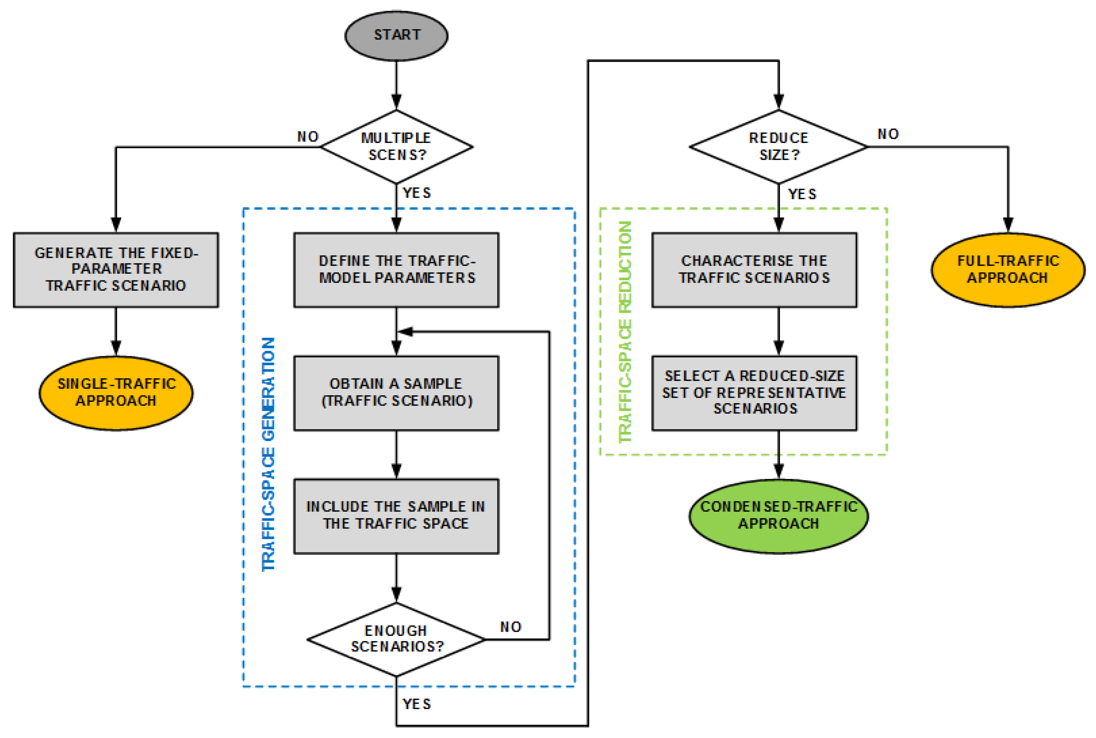
Figure 1 shows a flow diagram which represents different approaches to obtain a traffic model in these optimisation studies, with different levels of complexity. The first option is the one found in the literature, which includes just one traffic scenario, without uncertainties in the traffic variables (single-traffic approach). The computational burden associated with the obtainment of results will be the lightest possible, but the accuracy of the energy-saving results will probably be low.

Then, if stochastic variables are represented, the traffic model will include more than one traffic scenario per headway. In this paper, the traffic will be represented with some stochastic variables which follow certain probability distributions. The complex patterns in the operation of MTSs are included in a traffic space which contains a large-enough number of traffic scenarios. The details of the traffic space generation are given in Section 2. This option will lead to the highest energy-saving accuracy, but the computational burden will be the heaviest possible. It will be referred to as the full-traffic approach.

Finally, this paper proposes a novel traffic approach that will be named the condensed-traffic approach or representative-scenario approach. It consists of making an appropriate selection within the traffic scenarios included in the full-traffic approach. This selection requires a previous characterisation of the traffic scenarios, which is based on a novel function that projects rheostat losses to the locations in the line that are candidates to host infrastructure improvements. The condensed-traffic approach will contribute to improve infrastructure optimisation problems by including a large amount of traffic information with a low computational burden increase. The details of the traffic model’s size reduction are given in Section 3.

Table 2. Characteristics of the different traffic approaches.

Approach	Number of Scenarios	Accuracy	Computational Burden
Single traffic	●	Probably low	The lightest
Full traffic		The highest	The heaviest
Condensed traffic		Target: As high as possible	Target: As light as possible

summarises the characteristics of the three traffic approaches presented.

2. Traffic Model and Traffic Space Generation

This section covers the traffic space generation process, represented within a dashed blue rectangle in Figure 1. The process generates a set of traffic scenarios by obtaining samples of the stochastic variables that are identified to have the largest influence on the MTS traffic.

2.1. Traffic Model Parameters

For a given headway, there are certain traffic variables which may make it difficult to predict the line receptivity. This paper focuses on double-track lines with two terminal stations. In this kind of system, the main traffic variables affecting receptivity are:

• Dwell times at passenger stations. Even when the traffic controller allows trains to depart, several circumstances that are commonplace in an MTS (e.g., an unexpected surge of passengers at a certain station) may delay departure time. The work of [26] thoroughly studied dwell times in the Madrid Metro (Spain). The study found that dwell times at passenger stations (excluding traffic disturbances) follow log-normal distributions. This variation in the dwell times is expected to have a large influence on the synchronisation between a train’s motoring and braking phases, and therefore on the system’s receptivity. This paper applies a particularisation of the dwell time distributions presented in [26], which is given in

  Table 3. Factors included in the traffic model and values used in this study.

  Traffic Parameter	Model Used in the Study	Remarks
  Headway	4-, 7-, and 15-min headways	Three headways to cover the different traffic densities in the operation of the line.
  Dwell times at passenger stations	Log-normal distribution.
  Parameters:	Mean: 30 s.	Parameters tuned to represent the traffic in the line without dysfunctional situations.
  	Standard deviation: 3 s.
  	Minimum dwell time: 20 s
  	Maximum dwell time: 60 s
  Time shift between departure times at terminal stations	Uniform distribution from 0 s to the headway	Different time shift values to cover all the possible operation schedules.

  .
• The time shift between train departure times at terminal stations. The operation of double-track lines with two terminal stations is mainly determined by the headway between trains. However, the relative positions between the trains on both tracks are affected by the difference in time between the departures at the two terminal stations. This time shift between tracks influences the positions where trains cross each other, and so the moments (or time intervals) when it is easier for them to exchange power [27]. In the specific operation of an MTS, the nominal value of this variable may be known, and thus the specific schedule of the line would be determined. However, in general, this specific operation schedule may be varied by changing the time shift without affecting the service conditions (mainly determined by the headway). Consequently, in the generation of the traffic space, which aims to represent the long-term operation of the system, there is no reason to assign a greater probability to a certain time shift than to any other. Thus, it is reasonable to let the time shift between departures follow a uniform distribution from 0 s to the headway. It is important to note that each traffic scenario has a single time-shift value associated with it (see Table 3). e.g., Scenario 1: trains depart simultaneously from both terminal stations in the nominal case, and then the dwell time noise introduces small signal variations onto the actual departure times. Scenario 2: trains on track two depart 30 s later than those on track one, and then, again, the dwell time noise introduces variations.

Table 3 illustrates the factors included in the traffic model presented in this paper, which are known to affect the power exchange between trains. In addition, it shows the way they have been modelled in this study. It is important to note that the traffic scenarios in this paper include disturbances with respect to the scheduled operation plan, but the traffic is not so disturbed as to lead to dysfunctional situations that would require applying traffic regulation techniques to recover the proper operation of the line.

2.2. Traffic Space Generation

A traffic scenario is a sample of the total traffic space associated with a given headway. The expression of the total traffic space for the headway hw is given in Equation (1).

$$T{S}_{hw}=\left\{sce{n}_1(·),\dots ,sce{n}_E(·)\right\}$$

(1)

where $sce{n}_{\omega }(·)$ is the traffic scenario $\omega$, defined in Equation (2), and $E$ is the total number of scenarios in the traffic space.

$$sce{n}_{\omega }\left(shif{t}_{\omega },t{r}_{1,\omega }(·),\dots ,t{r}_{T,\omega }(·)\right)=\left\{sn{p}_1,\dots ,sn{p}_S\right\}$$

(2)

where:

• $shif{t}_{\omega }$ is the realisation of the time shift for the traffic scenario $\omega$, obtained with the probability distribution presented in Table 3.
• $t{r}_{t,\omega }\left(d{w}_{t,\omega }^1,\dots ,d{w}_{t,\omega }^{N\_EST}\right)$ is the evolution of the position and power for train $t$ in the traffic scenario $\omega$, which depends on the realisations of the stochastic dwell times ($d{w}_{t,\omega }^u)$ at all the passenger stations (from 1 to $N\_EST$). It must be noted that the dwell times are independent of the time shift and between them.
• $sn{p}_v$ is the snapshot $v$, which represents the sampling of the positions and powers of all the trains in the line for the time instant $v$. The sample time selected in this study equals 1 s.
• $S$ is the total number of snapshots included in the scenario (for one-second sampling time, the number of snapshots in a traffic scenario equals 60 times the headway in minutes).

The size required for the traffic space $(E)$ is not known a priori. This parameter is determined following a Monte-Carlo approach, such as the one used in [28]. It consists of increasing the number of scenarios in the traffic space until the mean and standard deviation of the main electrical variables defining each scenario are stabilised. These variables are: (1) energy consumption at traction SSs; (2) regenerated energy; (3) rheostat losses; and (4) conduction losses.

Figure 2 shows the stabilisation of these variables (obtained with the simulator) for a 7 min headway as the size of the dataset grows. In this paper, the size of the traffic spaces for the three headways under study include 300 scenarios.

3. Condensation of the Traffic Model

This section presents the method proposed in this paper to condense the traffic model included in the optimisation studies. The process is represented within a dashed green rectangle in Figure 1. The application of this method will make it possible to approximate the results that would be obtained with the whole traffic space ($T{S}_{hw}$) by means of a small number of representative scenarios. The fundamentals of this traffic space condensation are based on the analysis of the system’s electrical variables. Specifically, since energy savings are the key variable in the kind of studies covered by this paper, the method is based on the rheostat-loss reduction mechanisms presented in [29].

3.1. Characterisation of the Traffic Scenarios

The key to making the traffic-space condensation possible is to properly characterise the traffic scenarios. In particular, it is important that the characterisation captures the rheostat-loss events, representing not only the global rheostat loss figures, but also their distribution along the line and their frequency of occurrence. In addition, it was presented in [29] that there are obstacles to the absorption rheostat losses from certain locations, so it is essential to represent these interferences in the traffic scenario’s characterisation.

Each traffic scenario may contain a large number of rheostat loss events, which are the result of the complex interactions between trains. Then, there are several candidate locations to install devices to improve receptivity (RSs in this paper), which will be able to fully absorb some rheostat-loss events, but unable to reduce other ones. For these reasons, we propose a method that computes the projection of all the rheostat losses to all the candidate locations, which is based on the rheostat loss reduction mechanisms. Therefore, we assign to each traffic scenario a vector which contains as many values as there are RS candidate locations in the system (Equation (3)). Each of the elements in the vector contains the projection of all of the rheostat-loss events to the set of candidate locations (Equation (4)).

$$sce{n}_i\Rightarrow \left(\begin{array}{ccc}{a}_{i,1},& \dots & , a_{i,NLOC}\end{array}\right)$$

(3)

$$a_{i,loc}={\displaystyle \sum }_{r=1}^{R}R{P}_r(·)$$

(4)

where $i$ and $loc$ are respectively the traffic scenario and location under study (from 1 to $NLOC$); $R$ is the total number of rheostat-loss events that take place in the scenario $scen$; and $R{P}_r(·)$ is the Rheostat loss Projection (RP) function, which is proposed to represent the energy-saving potential associated with each pair of rheostat loss event and location. It is defined hereafter.

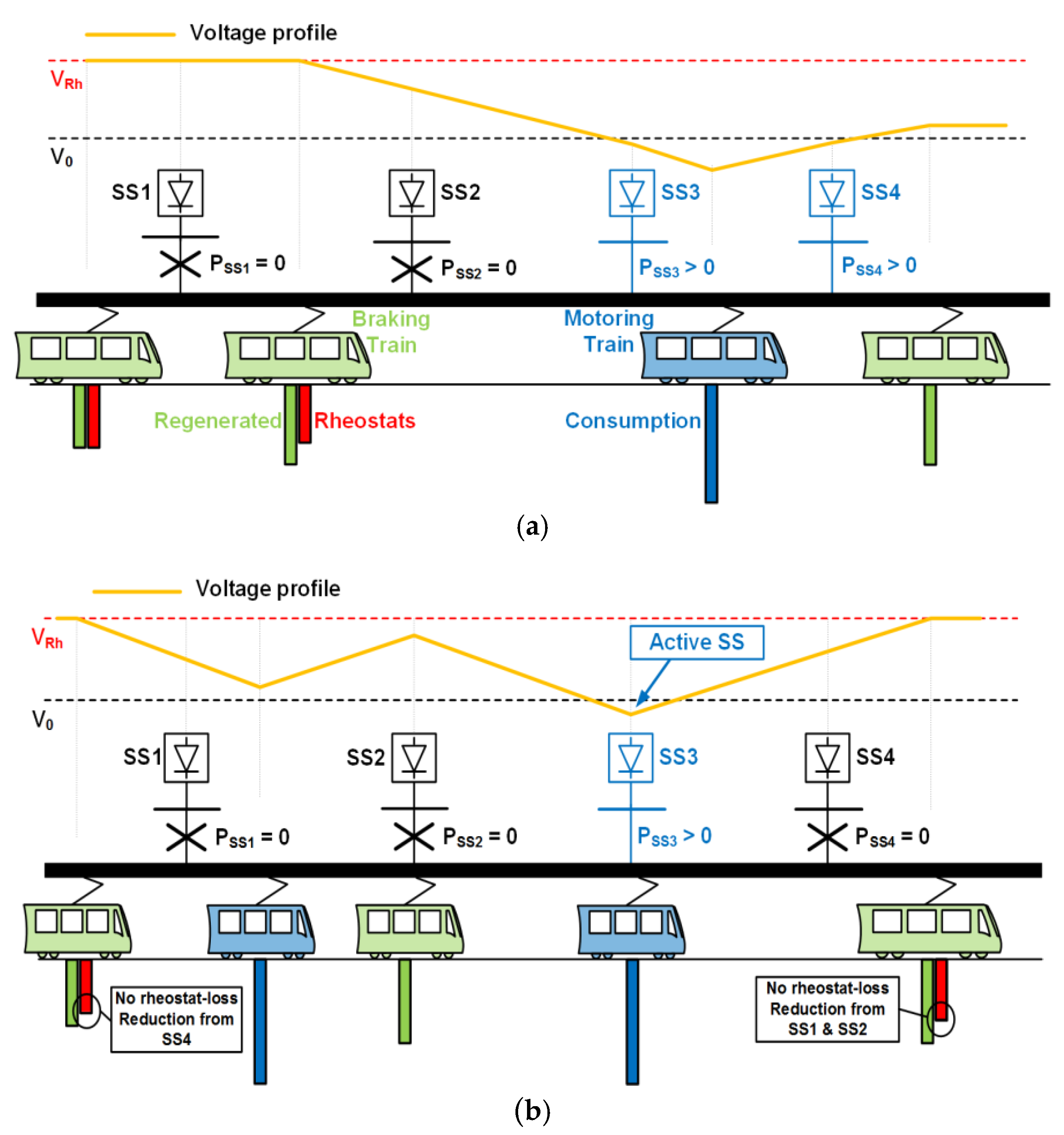
For each rheostat loss event and candidate location, it is required: (1) to identify whether it is possible to reduce the rheostat losses in this specific event from the candidate location under analysis; and (2) to detect the type of rheostat loss reduction mechanism to be applied.

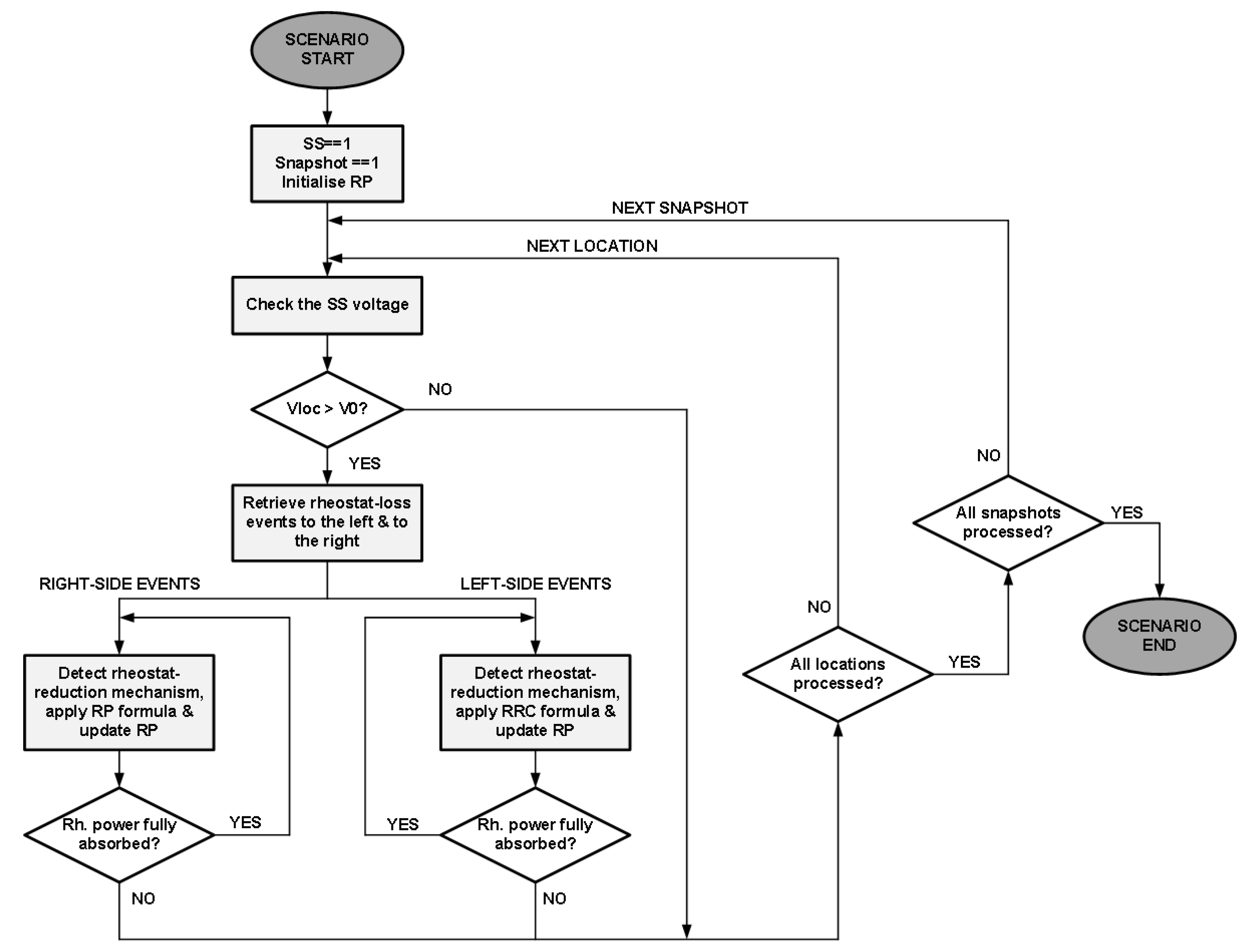
Figure 3 shows the flow chart followed in the characterisation of the traffic scenarios. It may be observed that the rheostat loss events are processed snapshot by snapshot. For each candidate location, the SS voltage is checked out to identify whether it is possible to absorb power from this location in this snapshot. In case it is possible, the rheostat-loss events to the left and right of the location are listed and sorted (the closest first). It is also important to note that, as was shown in [29], if there is an active (ON) SS between the RS candidate location and the rheostat loss event, it will be impossible to reduce these rheostat losses from that location. When this situation takes place, these events will be excluded from the list of rheostat loss events (0 RP value assigned). Then, the RP calculation starts.

The rheostat loss events are processed one by one. The type of rheostat loss reduction mechanism is detected, and the RP for this location is updated. If the RP calculation shows that the rheostat power in this event would not be completely absorbed, it can be concluded that the load flow beyond that train will remain invariant and no more rheostat loss reduction will take place. This process is carried out for both sides of the candidate location.

With respect to the RP formulae, it is important to note that, although it is not formally proven to be, the RP will usually be at a higher bound of the rheostat loss reduction attainable from a given location.

The expression applied to a rheostat loss event when the case (a) is detected is given in Equation (5).

$$RP\left(Er{h}_i,dr{h}_i,V_{loc}\right)=\min \left(\frac{V_{Rh}\left(V_{Rh}-V_{RS}\right)}{R_{l}dr{h}_i}\mathrm{\Delta }t,Er{h}_i\right)$$

(5)

where:

• $V_{loc}$ represents the voltage of the RS location in the load flow for the base system. The base system refers to the base configuration of the infrastructure, without any improvement.
• $V_0$ is the SS no-load voltage.
• $Er{h}_i$ is the energy lost in each rheostat loss event.
• $dr{h}_i$ is the relative position of the rheostat train with respect to the RS location $loc$.
• $V_{Rh}$ is the rheostat braking voltage threshold.
• $V_{RS}$ represents an hypothetical voltage in the RS location after the installation of the RS.
• $R_l$ is the resistance of the supply system, in Ω/km.
• $\mathrm{\Delta }t$ is the sampling time used in the traffic scenario generation.

The expression in Equation (5) represents a simplification of the power transmission from a $V_{Rh}$-volt voltage source to another point in the line in which voltage is clamped to a certain level. This expression does not aim to be an accurate representation of the actual load flow, but a simplified means to rapidly obtain the potential rheostat loss reduction from the RS location. As can be observed, the RP value is limited to the magnitude of the rheostat loss event and then normalised.

When the case (b) is detected, the RP is calculated following Equation (6).

$$RP\left(Er{h}_i,dr{h}_i,V_{loc}\right)=\min \left(\frac{V_{Rh}\left(V_{Rh}-V_{RS}\right)}{R_{l}dr{h}_i}·\frac{V_{loc}-V_{RS}}{V_{Rh}-V_{RS}}\mathrm{\Delta }t,Er{h}_i\right)$$

(6)

From the analysis of Equation (6), it may be extracted that the RP function represents the rheostat loss reduction when the RS is in a power exchange path by modulating the expression in Equation (5) with a coefficient between 0 and 1: $\left(V_{loc}-V_{RS}\right)/V_{Rh}-V_{RS}$). This coefficient will naturally tend to 1 when the RS location is close to the rheostat train (the voltage in the base system is close to the rheostat threshold) and to 0 when it is close to the motoring train (or an active SS). With this modulation, it is possible to obtain an approximate figure of the actual rheostat loss reduction.

Finally, Equation (7) presents the RP expression applied when case (c) is detected.

$$RP\left(Er{h}_i,dr{h}_i,V_{loc}\right)=\min \left(\frac{V_{BTr}\left(V_{BTr}-V_{RS}\right)}{R_l{d}_{BTr}}·\frac{V_{loc}-V_{RS}}{V_{BTr}-V_{RS}}\mathrm{\Delta }t,Er{h}_i\right)·f_{ON\_SS}$$

(7)

where:

• $V_{BTr}$ is the voltage of the braking train that is causing the high base system RS location voltage. It must be noted that in this case, this train is not in rheostat mode.
• $d_{BTr}$ is the distance between the braking train that is causing the high base system RS location voltage and the RS location.
• $f_{ON\_SS}$ is a binary factor which is set to zero if there is an active (ON) SS between the rheostat train under study and the RS location. This is used to represent the decoupling effect of active SSs that was presented in [29].

The expression in Equation (7) is applied when there are no active SSs between the rheostat loss train and the RS location. When there is an active SS between the rheostat event under study and the RS location, the rheostat loss reduction is marginal, and the RP function is consequently set to zero.

Application Example

The application of this scenario characterisation is here illustrated with an example. Let us consider the traffic scenario $i$, which is made up of the two snapshots presented in Figure 4a,b. They will be named snapshot 1 and 2. The characterisation of this traffic scenario for the four RS candidate locations in this example will be carried out by analysing the four rheostat loss events (two in snapshot 1 and two in snapshot 2), which will be ordered from left to right.

Table 4. Classification of the rheostat loss events for each candidate location in the application example.

Application Example		Candidate Location
		SS 1	SS 2	SS 3	SS 4
Rh. Event	1 (Snp 1)	Left 1. Type a	Left 1. Type b	N/A	N/A
	2 (Snp 1)	Right 1. Type a	Left 2. Type b	N/A	N/A
	3 (Snp 2)	Left 1. Type b	Left 1. Type c	N/A	N/A
	4 (Snp 2)	N/A	N/A	N/A	Right 1. Type b

shows the results of the classification and detection of the reduction mechanism for all of the rheostat loss events in relation to all of the candidate locations. The characterisation value assigned to location 1 ($a_{i,1}$) will be the sum of the RP values for the rheostat loss events 1 to 4. The first two values will be obtained with Equation (5) (reduction case a). The value for the third event will be obtained by applying Equation (6), and the fourth event will have 0 RP value, for there is an active SS (SS3) between the event and the candidate location.

In the case of the value for location 2 ($a_{i,2}$), the rheostat loss event 2 will only be computed if the RP value for event 1 hits its maximum value (all the rheostat losses in event 1 are absorbed). Then, it is also important to note that $a_{i,3}$ will be 0, provided that this SS is in ON mode at both of the two snapshots in the traffic scenario.

The calculation of $a_{i,4}$ follows the same reasoning. Rheostat events 1, 2, and 3 are set out of the characterisation because SS3, in ON mode, does not allow for the reduction of losses from location 4.

3.2. Representative Scenario Selection

The selection process is based on the RP characterisation presented, and on its correlation with energy savings, which will be checked out in Section 4.2. It aims to reduce the size of the traffic input to an MTS optimisation study, preventing it from using 300 scenarios for each traffic space.

The strategy proposed to perform this size reduction is: a set of traffic scenarios are selected to be representative of the traffic space if, for all of the RS locations, the average RP values of the reduced set are close to the average RP values of the total traffic space.

In this paper, the threshold to classify whether the average RP values of both sets are close enough has been set to ±5%. This value has a strong relation with the desired energy-saving accuracy. If a more restrictive threshold is selected (e.g., 3%), the representative scenario set will contain more traffic scenarios, and vice-versa.

4. Results

In this section, we apply the traffic model presented in the paper to a case study line. After the presentation of the case study in Section 4.1, we analyse the accuracy of the condensed traffic approach for different sizes and subgroups of traffic scenarios within the total traffic spaces with respect to a random scenario selection approach (Section 4.2). Then, in Section 4.3, we carry out a comprehensive energy-saving accuracy analysis, where we first use a test to verify that the method is accurate for all of the candidate locations, and then we test its generalisation capability by measuring the accuracy for different infrastructure configurations.

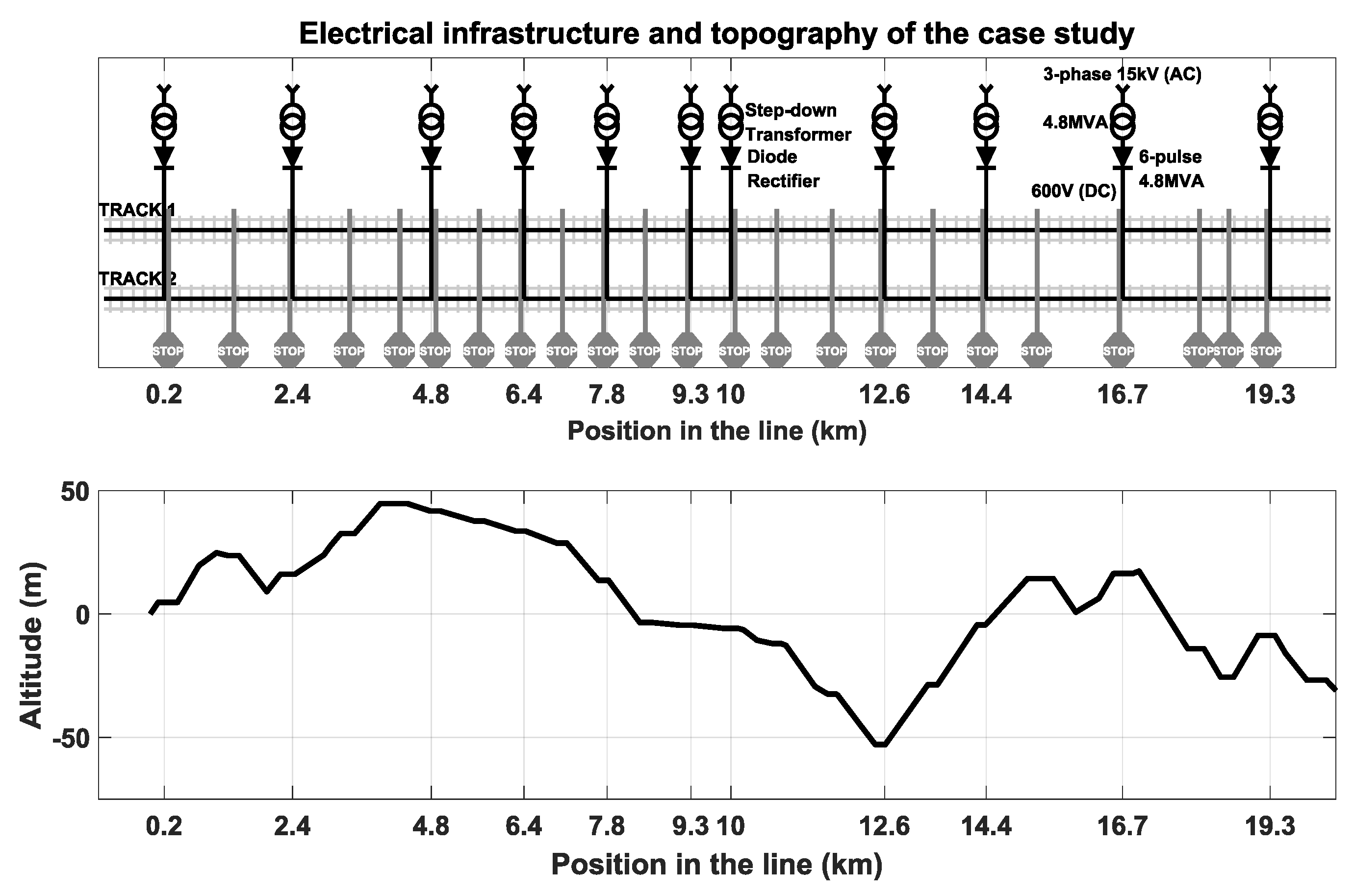
4.1. Case Study Line and Definitions

All of the results in this paper have been obtained by means of an electrical multi-train simulator developed in the Institute for Research in Technology (Comillas Pontifical University, Madrid, Spain). Its details may be found in [2].

The traffic model presented in the paper has been applied to the same case study line that was analysed in [29]. The reader is invited to consult this reference if interested in the particular details of the line. Nevertheless, Figure 5 has been reproduced to concisely present the SS number and locations, and the line topography.

Table 5. Specific values for the RP function parameters.

RP Parameter	Selected Value	Remarks
VRh	710 V	10 V lower than the maximum pantograph voltage allowed.
VRS	646.4 V	640 V + 1%
Rl	22.4 mΩ	Active and return line impedance

presents the specific values used for the RP parameters presented in Section 3.

Three headways (4-, 7-, and 15-min headways) have been used to study the accuracy of the traffic model proposed. These headways represent peak hour, off-peak hour, and sparse traffic conditions, respectively. They are intended to show that the traffic approach in the paper suits all of the different traffic conditions in the line. For each headway, a traffic space containing 300 traffic scenarios has been generated. The energy savings obtained with these traffic spaces are used as the base case for the error calculations.

The error definitions, the single RS test, and the multiple RS test presented in [29] are also used in the energy-saving accuracy analyses throughout this paper.

4.2. Condensed Traffic Model: Correlation and Size Results

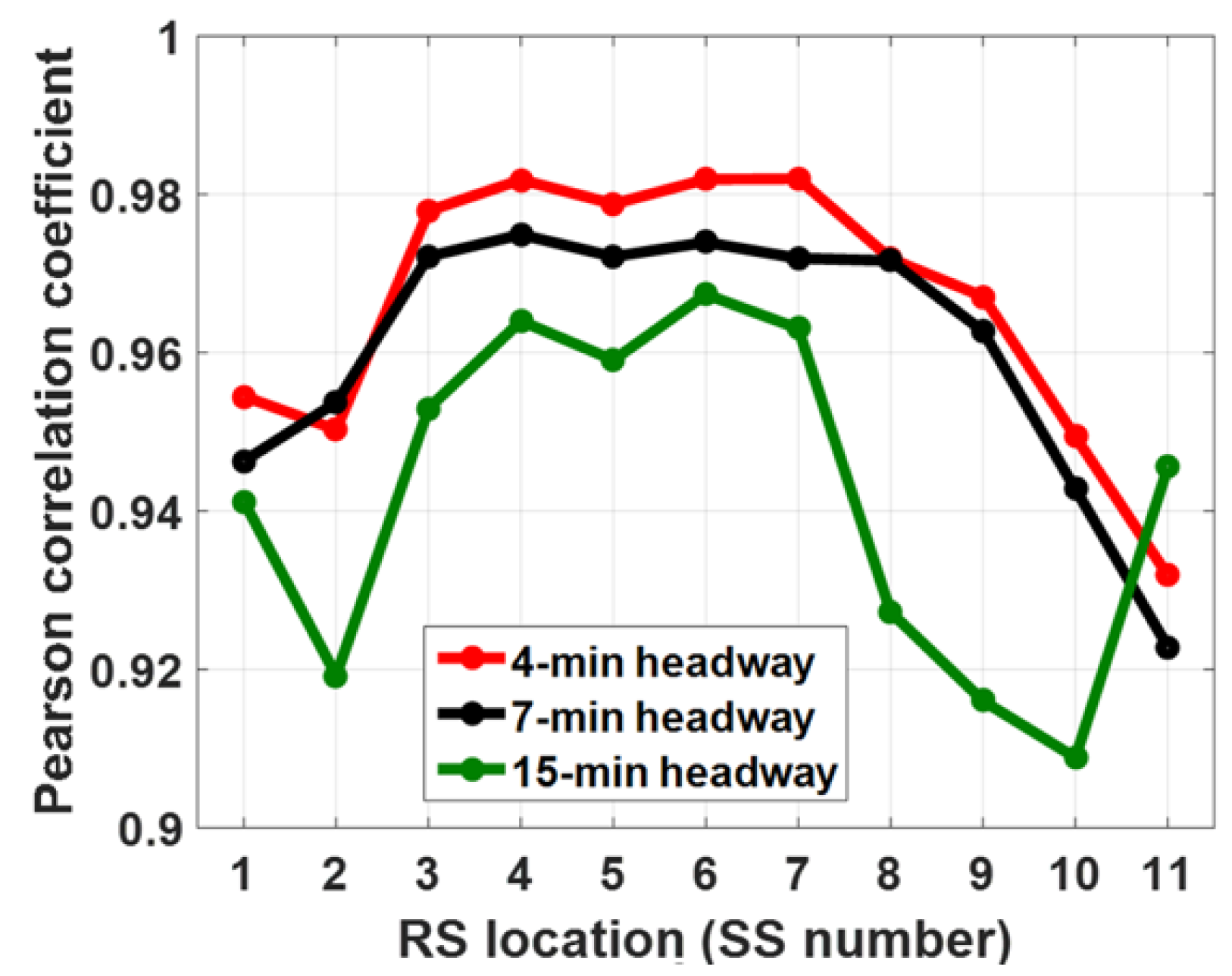
4.2.1. Correlation between the RP Values and Energy Savings

Figure 6 presents the correlations between the RP values and the energy savings obtained for each RS location in the single RS test. The 300 scenarios generated in Section 2.2 have been included in this analysis. It may be observed that the correlations are greater than 0.9 for all the RS locations (fairly significant). The results for the 4- and 7-min headways are very similar, representing high correlation results. The results for the 15-min headway tend to be worse, but are still greater than 0.9 for all of the RS locations.

Based on these high correlation results, it can be stated that the traffic scenario characterisation proposed is a good candidate to guide the traffic model size reduction process.

4.2.2. Traffic Model Size Reduction Results

This section assesses the required number of traffic scenarios that the condensed traffic model should include. Two approaches are compared:

• The representative scenario selection proposed in the paper, where the traffic scenarios are characterised by means of the RP function.
• A random selection process where scenarios are grouped without information.

The method to analyse the number of scenarios required consists of making random combinations of scenarios of increasing size. In the case of the representative scenario selection, a combination of scenarios is only accepted if it accomplishes the criterion explained in Section 3. In the case of the random selection process, since there is no information on the adequacy of the selection, all of the combinations are accepted. For each condensed traffic size and approach, 1000 samples are obtained to have statistically significant results.

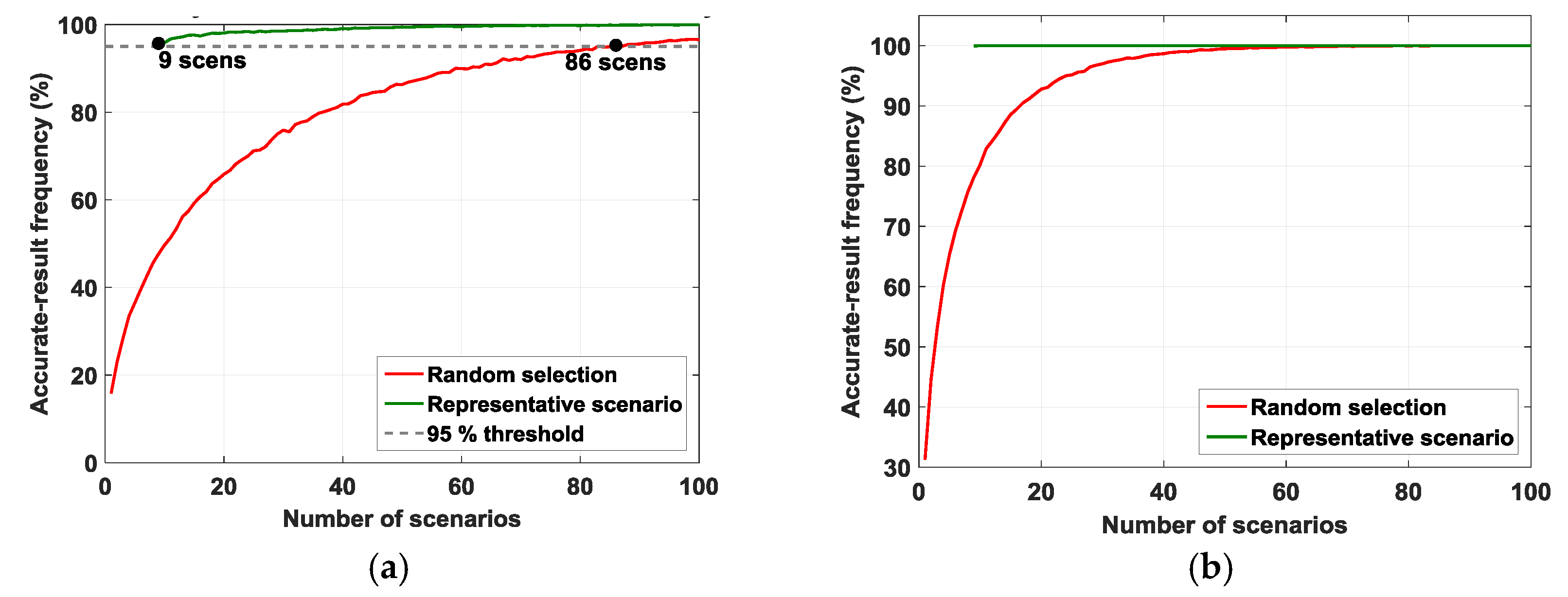
Then, the single RS test is applied and the mean energy-saving results obtained are compared with the total traffic space results (the base case). The energy-saving results are classified as accurate if they are within a ±5% error band around the total traffic space savings, and the proportion of accurate instances is calculated. The same process is replicated for a ±10% error band to assess the probability of having extremely inaccurate results. e.g., for the case of the combinations of 20 scenarios, when the RP function method is used to obtain them, Figure 7a shows that around 97.5% of the cases lead to energy-saving errors lower than 5%. When the scenarios are selected without previous information, only 66% of the cases would fulfil this accuracy criterion. Then, Figure 7b shows that all of the combinations obtained with the RP method lead to errors lower than 10%, whereas for the random selection, 8% of the combinations exhibit errors larger than 10%.

When the RP function is used to guide the representative scenario selection, Figure 7a shows that, for the 7-min headway, the acceptance criterion defined is not fulfilled until nine scenarios are combined. Using this method, more than 95% of the energy-saving accuracy results are within the 5% error band. Then, Figure 7b (green curve) shows that all of the cases outside this error band exhibit relative energy-saving errors lower than 10%.

These size results represent a dramatic reduction with respect to the random selection size. It may be observed in Figure 7a that, for the same accuracy standard, the required size with this method equals 86 scenarios. In addition, it is highly possible to have extremely poor results (relative error larger than 10%) until around 40 scenarios are selected, as shown in Figure 7b.

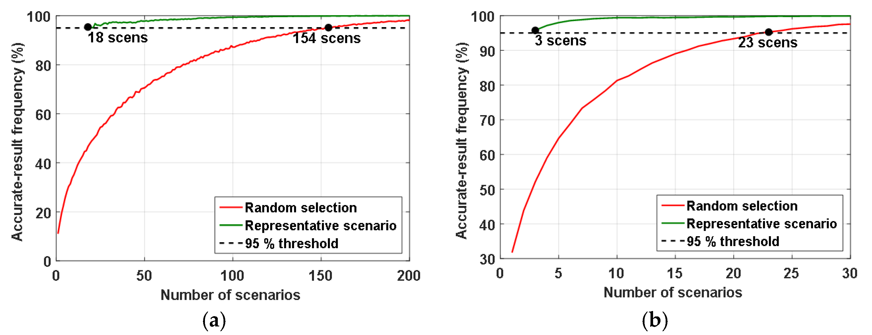
Figure 8 shows the extension of these results to the 4- and 15-min headway cases. The results are qualitatively similar, including for the 10% error analysis, which has been omitted for the sake of clarity. The representative scenario accuracy results obtained with the method proposed in this paper have been shown to be acceptable with a set size much lower than the one required with a general selection approach.

These representative scenario set sizes will be used in Section 4.3 and Section 4.4 to confirm the accuracy results, and to illustrate the computational burden concerns associated with each selection method.

4.3. Energy-Saving Accuracy Results

The energy-saving results’ accuracy will be measured by applying first the single RS test. This test is aimed at analysing the goodness of the representative scenarios location by location. Then, the multiple RS test is applied to verify the accuracy for generalised infrastructure improvements.

Table 6. Relative error results for the single RS test.

Error Results	RS loc. (SS)	1	2	3	4	5	6	7	8	9	10	11
4 min	Savings (kWh/h)	127	129.3	80.3	90.8	97.8	96.6	91.6	103.7	103.9	130.2	154.5
	ε. Repr scen (%)	−1.3	0.9	−1.7	−3.7	0.2	−0.1	−4	−4.2	−1.3	−2	2.2
	ε. Single scen (%)	−8.5	−11.9	−3.8	−9.6	−11.8	−10.6	−11.2	−73.2	−74	−33.1	13.7
7 min	Savings (kWh/h)	130.1	149	134.6	125.3	128.3	128.8	126.5	127.1	114.6	131.5	142.8
	ε. Repr scen (%)	3.5	2.5	3.5	4.1	2.1	−1.1	−3.1	−2.9	−2.2	−4.7	1.6
	ε. Single scen (%)	1.4	−15.4	−51.1	−42.4	−56.4	−62.1	−60.5	−69.5	−46.8	−27.1	−28.2
15 min	Savings (kWh/h)	123.6	149.2	156.8	152.6	149.7	146.7	145.7	163.8	162.6	164.4	140
	ε. Repr scen (%)	−4.1	−4.4	−2.2	−3.2	−4	−3.8	−4.1	3	2.4	4.2	3.1
	ε. Single scen (%)	5.6	15.2	11.1	1.1	−15.6	−23	−16.1	25.8	31.7	6.8	3.3

presents the relative accuracy figures obtained with the single RS test, together with the average energy savings for each traffic space. Table 6 compares the results obtained with: (1) the representative scenario traffic approach proposed in this paper; and (2) the traffic model usually implemented in the literature, which consists of using a single traffic scenario (see Figure 1 in Section 1.1). The reference used is the full-traffic approach presented in Section 1.1 and developed in Section 2.2. Percent error results greater than 10% have been represented in red.

On the one hand, it may be observed that, for all headways, all of the RS locations exhibit relative errors lower than 5% for the representative scenario traffic approach. This means that the representative scenario selection approach presented in the paper is accurate for all of the zones in the line and headways.

On the other hand, it may be observed how the single scenario approach fails to obtain accurate energy-saving results for all headways under study. The accuracy results are especially poor for the 4- and 7-min headways, whereas it obtains better results for the simpler traffic situations in the 15-min headway. Nevertheless, for all headways it presents relative energy-saving error figures greater than 10%.

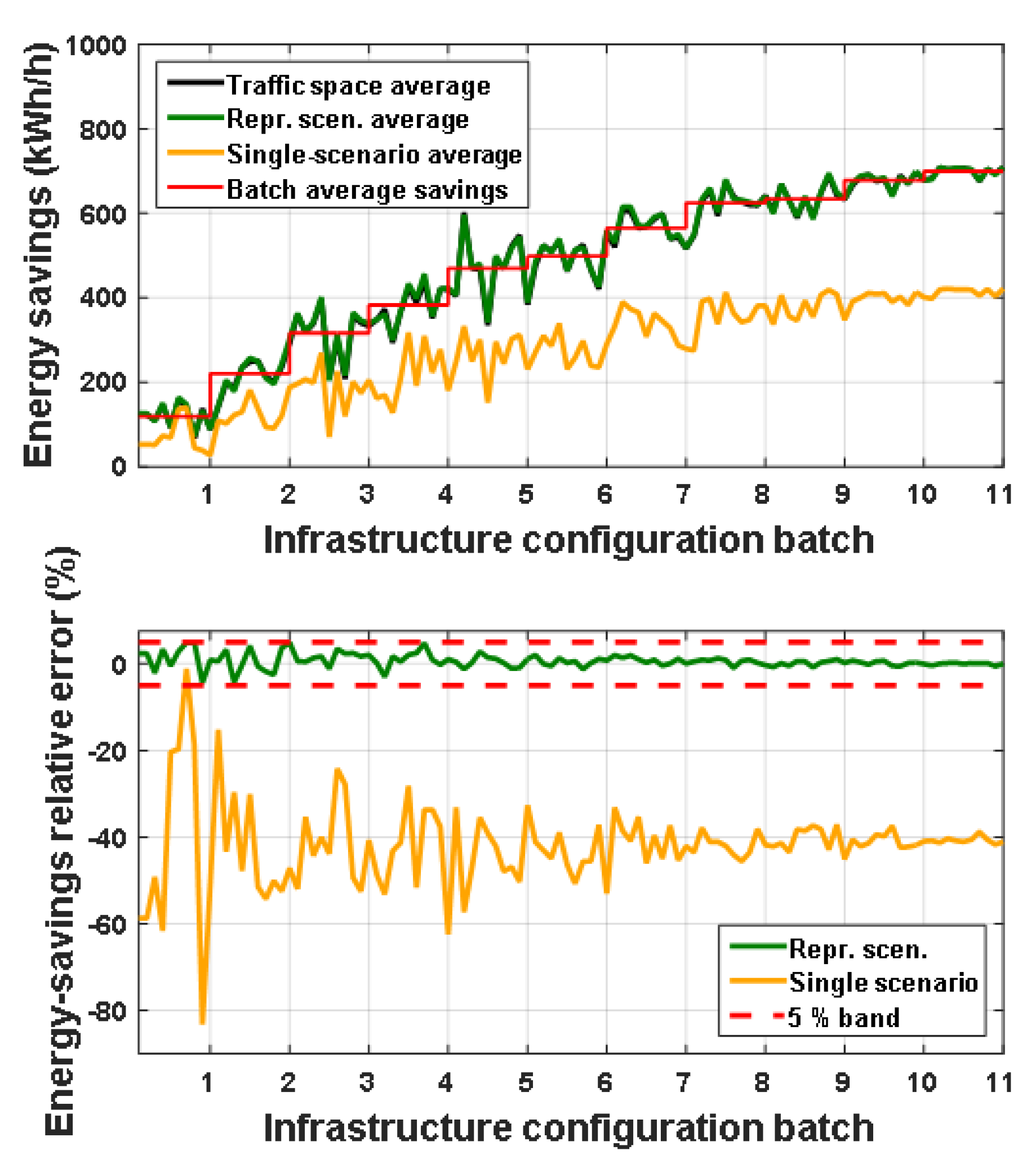
Once the single RS test has shown that the representative scenarios selected are accurate for all of the candidate RS locations, Figure 9 presents the energy-saving results obtained in the 110 RS configurations of the multiple RS test for the 7-min headway case. It represents both the results obtained with the representative scenarios and with the single scenario traffic approach. It may be observed in the top-side graph that the results obtained with the representative scenarios are close to the reference values (obtained with the whole traffic space). The results from the single scenario traffic approach differ substantially from the reference values.

The bottom-side graph in Figure 9 shows the relative errors. It must be observed that the accuracy results are inside the accepted tolerance for the representative scenarios. The errors obtained with the single scenario traffic approach are inside the accepted tolerance band only in one out of the 110 configurations in the multiple RS test. For high energy savings, it tends to stabilise around 40% error. The reason for this effect is that the total rheostat loss values in the scenario used in this simplified approach are lower than the average total rheostat loss values of the whole traffic space.

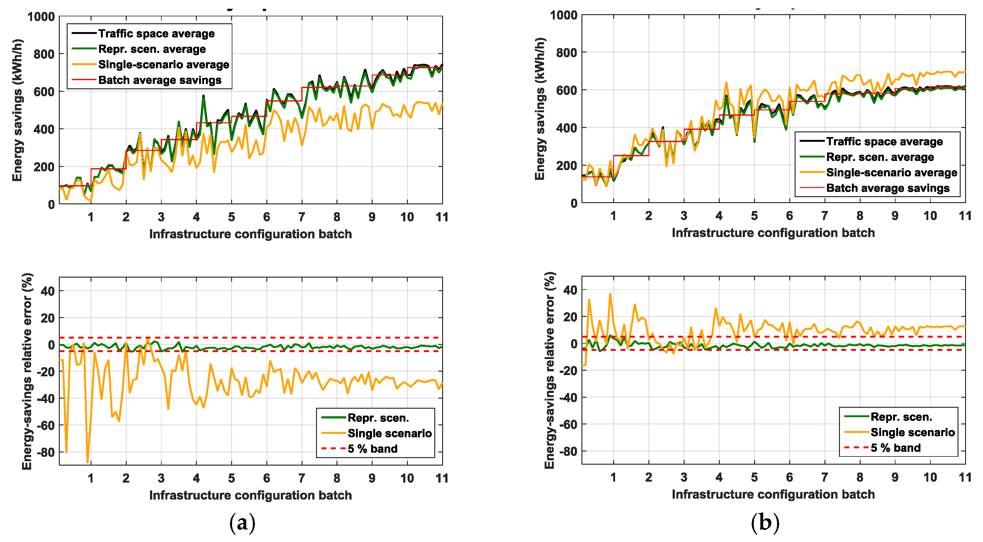
Figure 10 shows the extension of the multiple RS test for the 4- and 15- min headways. The results obtained with the representative scenarios are qualitatively better than those yielded by the single scenario traffic approach. The errors for the latter are again unacceptable. These results show that there is a large uncertainty about the energy-saving results to be obtained with the single scenario traffic approach. They are always inaccurate, and they may be larger or smaller than the actual reference values.

4.4. Computational Burden Analysis

The details of the optimisation model are outside the scope of this paper. For this reason, the optimiser presented in [16] has been used as a reference for obtaining computation time results. That work implements a genetic algorithm to search for optimum infrastructure configurations. This population-based algorithm has been parameterised with 40 elements and 100 generations. Thus, to obtain the optimum infrastructure configuration, the optimisation process requires 4000 simulations of the system at the different headways included in the traffic model. It is important to note that the relative computation time savings associated with the representative scenario approach would be conserved for other optimisation algorithms, which may take less or more simulations to obtain the optimum infrastructure solution.

The traffic model and the computation times in [16] have been replaced by the model in this paper and the simulation times obtained with our simulator. The average simulation times measured for a single traffic scenario are 0.77 s, 1.31 s, and 2.73 s for the 4-, 7-, and 15-min headways, respectively. The computation times required to generate the elements in the population and to apply the genetic algorithm’s rules are in the range of milliseconds, and have been consequently neglected. The machine used to perform the simulation campaign features an Intel(R) Core(TM) i7-2600 [email protected] GHz processor and 8 GB RAM memory.

With this information, it is possible to compare the optimisation times and accuracies for the three traffic approaches defined in this paper. For the full-traffic approach, this analysis uses the number of scenarios obtained in Section 4.2 instead of all 300 scenarios per headway obtained in Section 2.2. This aims to make a fairer analysis of the computation time advantages associated with the application of the selection process presented in this paper.

These results are presented in

Table 7. Optimisation process characteristics for the three traffic approaches analysed.

Characteristics of Traffic Approaches		Single Traffic	Condensed Traffic	Full Traffic
Energy-saving error		Unacceptable	<5%	0
Number of scenarios	4-min	1	18	154
	7-min	1	9	86
	15-min	1	3	23
Computation time		5.4 h	37.2 h	323.5 h

. The main conclusions to be drawn are:

• The single traffic approach is, of course, the less demanding traffic model in computational terms. However, its energy-saving accuracy is too low to trust the results obtained.
• For the required 5% energy-saving accuracy, the random selection of traffic scenarios within the total traffic spaces makes the optimisation time soar dramatically. It would take around two weeks to perform the optimisation process with this traffic approach.
• The RP function-characterised selection of representative scenarios proposed in this paper leads to an 88% reduction in the expected optimisation time with respect to the random selection case. The optimisation time is around 7 times larger than the one with the usual approach in the literature, but this time increase is necessary to obtain reliable energy-saving results.

5. Conclusions

This paper has presented a method to obtain a condensed traffic model for MTS electrical infrastructure optimisation studies. The method represents an evolution of the classical traffic approach in the railway optimisation literature, which consists of using a fixed deterministic dwell time at stations for the generation of a single traffic scenario per headway.

This condensed set of representative scenarios are selected from a general stochastic traffic space in a novel approach. The traffic condensation is attained by performing a characterisation of the traffic scenarios based on a function that projects rheostat losses to a set of locations in the line. This novel characterisation function is based on a rheostat loss reduction mechanism frame previously proposed by the authors.

The accuracy in the representation of energy savings with the traffic approach proposed in the paper has shown to be high for different infrastructure configurations and traffic headways. This approach has been shown to represent a qualitative accuracy increase with respect to the single scenario approach.

In the future, this traffic modelling approach will be applied to other types of systems. The representation of disturbed traffic conditions under different signalling systems (CBTC, ERTMS, etc.) could also complement the model presented in this paper, as well as the definitions of the changes required to adapt the model to ESSs.