Windbreak Effects Within Infinite Wind Farms


1
Department of Mechanical Science and Engineering, University of Illinois, Urbana, IL 61801, USA
2
Department of Civil and Environmental Engineering, University of Illinois, Urbana, IL 61801, USA
3
Department of Aerospace Engineering, University of Illinois, Urbana, IL 61801, USA
*
Author to whom correspondence should be addressed.
Energies 2017, 10(8), 1140; https://doi.org/10.3390/en10081140
Submission received: 9 May 2017
/
Revised: 14 July 2017
/
Accepted: 27 July 2017
/
Published: 3 August 2017
(This article belongs to the Collection Wind Turbines)
Abstract
:Building upon a recent study that showed windbreaks to be effective in increasing the power output of a wind turbine, the potential of windbreaks in a large wind farm is explored using simplified formulations. A top-down boundary layer approach is combined with methods of estimating both the roughness effects of windbreaks and the induced inviscid speed-up for nearby turbines to investigate power production impact for several layouts of infinite wind farms. Results suggest that the negative impact of windbreak wakes for an infinite wind farm will outweigh the local inviscid speed-up for realistic inter-turbine spacings, with the break-even point expected at a spacing of ∼25 rotor diameters. However, the possibility that windbreaks may be applicable in finite and other wind farm configurations remains open. Inspection of the windbreak porosity reveals an impact on the magnitude of power perturbation, but not whether the change is positive or negative. Predictions from the boundary-layer approach are validated with power measurements from large-eddy simulations.
1. Introduction
In recent years, increased efforts have been carried out to optimize the energy harvested by turbines within wind farms by manipulating the interaction between the turbines and the atmospheric-boundary-layer flow. Included in these concepts is wind farm layout, exemplified by Chamorro et al. [1], who observed an increase on the order of 10% in power production for a staggered versus an aligned wind farm due to greater wake decay between turbines. The spacing between turbines has also been investigated by Meyers and Meneveau [2], who suggested that the optimal distance between turbines may be greater than is commonly practised. The impact of topography has also proved to be an important factor in wind farm layouts, as winds are accelerated at the crests of hills, which may be exploited to harvest greater power from a turbine [3]. The use of different-sized turbines within a wind farm has also been investigated by Chamorro et al. [4], who observed enhanced downward momentum flux when two different sizes of turbines were used. Redirecting turbine wakes so as to avoid interference with downwind turbines has also been shown to be useful, with several methods discussed by Fleming et al. [5]. In recent years, there has also been increasing evidence that rougher ground surfaces may be beneficial to the operation of a wind farm, due to enhanced turbulent mixing leading to faster wake recovery. Recently, Xie et al. [6] showed that adding small, vertical-axis turbines among larger horizontal-axis turbines had the potential to increase the power output of the larger turbines by 10% due to faster wake recovery. Chamorro et al. [4] showed experimentally that a rough surface led to higher wake mixing and more diffused momentum deficits. However, the impact on wake recovery is not the only effect to be considered. Tobin et al. [7] recently demonstrated the usefulness of windbreaks (typically rows of trees or fence structures) in diverting low-level flow to the level of a wind turbine rotor, where a significant increase in power production was shown to agree well with linear theory. However, the impact of the windbreak wake on the power production of downwind turbines remains unclear.
The combined impacts of the inviscid speed-up from flow over windbreaks and the enhanced mixing and greater velocity deficits in their wakes are expected to be strongly dependent on wind farm layout. The applicability of windbreaks in wind farms may therefore not be universal. For instance, Denholm et al. [8] showed several typical wind-farm-layout strategies. In a single string configuration, where turbines are only rarely in the wakes of others, the single-turbine analysis of Tobin et al. [7] should be broadly applicable. However, other cases (e.g., the parallel-rows and cluster configurations) require an accounting for windbreak wakes. An appropriate candidate for predicting the negative impact of windbreaks in a wind farm is the top-down model of wind farm boundary layers first proposed by Frandsen [9] and later expanded upon by Calaf et al. [10]. Within this framework, the negative impacts of windbreaks can be parametrized as a greater surface roughness, which is expected to decrease hub-height wind speeds. The top-down model has proven valuable in the investigation of a wide variety of wind-farm topics, including the economic optimization of inter-turbine spacing [2] and the impact of small vertical-axis turbines among larger horizontal-axis counterparts [6].
Here, we augment the top-down model with roughness effects of windbreaks and the induced flow speed-up in a combined formulation. In addition, we explore the case of an idealized infinite wind farm with several layouts. The employed theory is outlined in Section 2, and an application is presented in Section 3.
2. Integrated Boundary-Layer Theory for Windbreak Effects in Wind Farms
A method to make predictions of turbine power output in a wind farm that has windbreaks is established using an approach based on the top-down model of wind-farm boundary layers. We consider an infinite array of wind turbines with rotor diameter D and hub height , spaced and in the streamwise and transverse directions. We also consider that a windbreak of height h and transverse width b is placed facing the direction of mean flow a short distance (∼5 h) upwind of each turbine. A schematic of the concept is shown in Figure 1.
2.1. Drag Partition for Wind Turbines and Windbreaks
Above a wind farm with windbreaks, the total kinematic shear stress, , can be split up into its contributions from the ground, , the windbreaks, , and the wind turbines, ; i.e.,
For a steady flow, this total stress must be in equilibrium with large-scale forcing; namely, a pressure gradient or geostrophic wind.
2.1.1. Surface Stress and Windbreak Drag
For wide streamwise spacings , the flow near the ground is assumed to come to equilibrium with the surface roughness in the distance between windbreak/wind turbine pairs, and the equilibrium stress on the ground is . However, because of the body and recirculation zone of the windbreak, the areally averaged ground shear stress is less than , and is well modelled according to Arya [11] as:
where and is the fraction of the frontal silhouetted area of the windbreak to the ground surface. A result of the assumption that the near-ground flow reaches equilibrium between turbines is that the flow approaching the windbreaks is logarithmic of the form:
where is the von Kármán constant and is the aerodynamic roughness length of the underlying ground. The drag contribution of the windbreak can then be parametrized with an areal drag coefficient , where is the drag coefficient of the windbreak and . Then, may be written as:
In the vertical region between windbreak and wind turbine, the flow is also assumed logarithmic, with a friction velocity and roughness length . As the surface shear and the drag from the windbreaks add in this region, the friction velocity here is inferred by combining Equations (2) and (4), with the result:
With a relation between and , can be found if the height where the two logarithmic profiles match is determined. Arya [11] took this height as that of an internal boundary layer which grew over the distance between obstacles, and arrived upon the following result for :
2.1.2. Turbine Thrust
Similar to the treatment of the windbreaks, the turbine thrust may be parametrized with a planform thrust coefficient , where is the turbine thrust coefficient, so that the areal turbine thrust can be written as:
Several different methods exist for estimating . The most basic of these approaches is that of Frandsen [9], which uses the spatially averaged velocity (spatial averaging denoted as ) and assumes logarithmic velocity profiles below and above the hub height:
In Equation (9), is the roughness height measured above the level of the turbines. Because the total shear stress above the turbines must be equal to the sum of the shear below and the turbine thrust, Equation (1) can be written as:
By enforcing continuity of the velocity profile at , the following expression for based on known and prescribed quantities is obtained:
With known, can be estimated from Equation (9), and a prediction of the power output can be made as . However, the velocity profile assumptions of two logarithmic layers which meet at is not consistent with observations, which show a significant deviation from a logarithmic profile over the vertical extent of the turbine rotor. Calaf et al. [10] proposed a wake-enhanced model, which adds a wake layer over this region parametrized by a non-dimensional wake eddy viscosity, , based on an assumption of 1 m, and = 100 m. They present an equation for of:
and arrive upon the following expression for (see Calaf et al. [10] for details):
Calaf et al. [10] effectively showed that their approach gives an improved estimate of over the simpler approach taken by Frandsen [9]. However, both models estimate the turbine thrust and power based on the horizontally averaged value , which may be significantly different than the actual velocity approaching a wind turbine. Further, neither one differentiates between streamwise and spanwise spacing. This has typically been addressed by matching a top-down model with a wake model, producing an estimate for an “effective” spanwise spacing as discussed in Stevens et al. [12], who proposed such a combined model with good results. This effective spacing is typically lower than the true spacing. Similarly, Yang et al. [13] introduced a combined top-down and wake model, and found it to be in greater agreement with their data than a simple boundary-layer model.
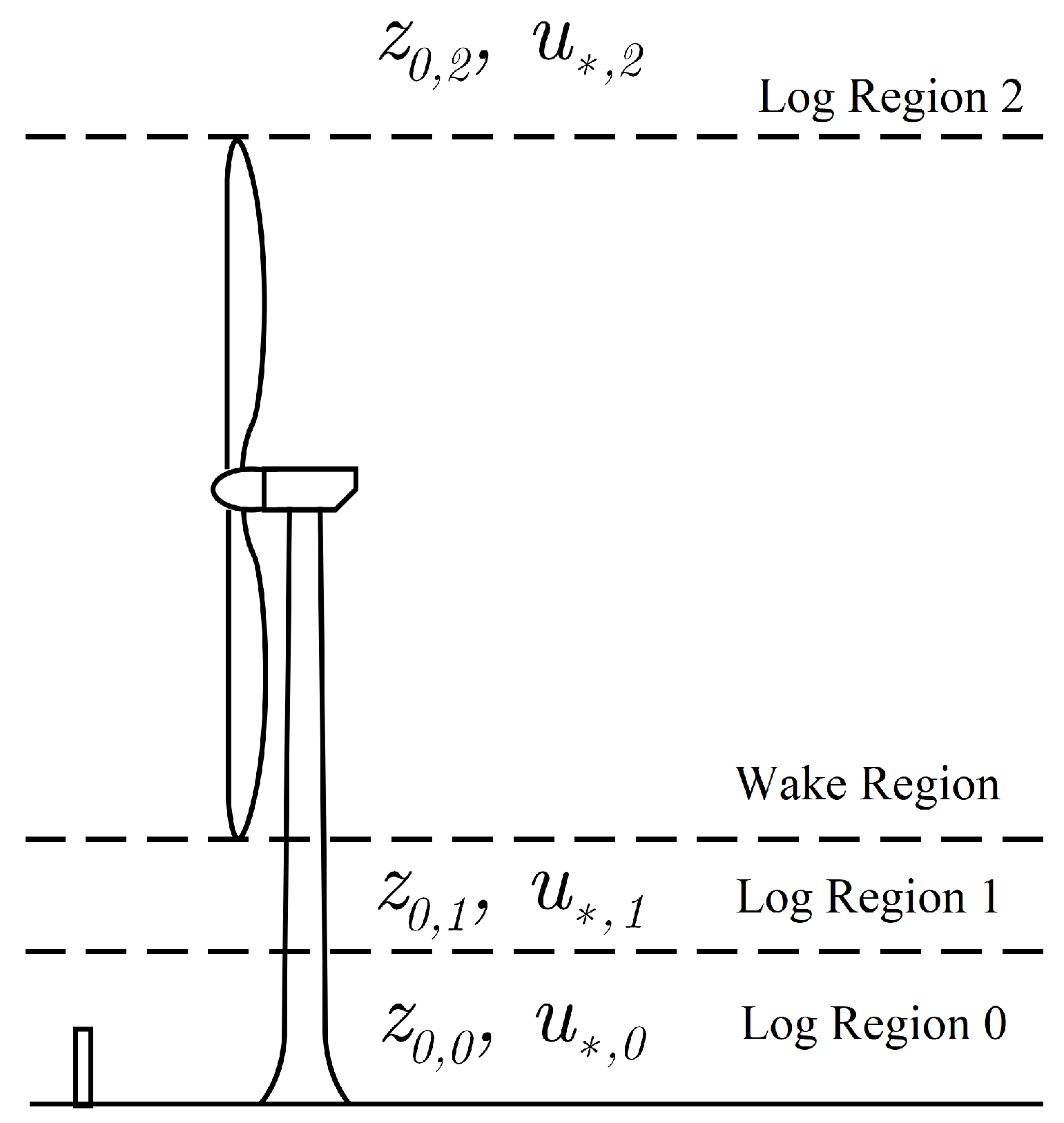
To summarize, we will proceed with the assumption of two logarithmic regions below the turbine rotor, a wake region over the vertical extent of the rotor using the method of Calaf et al. [10], and a third logarithmic region above the turbine. The several assumed flow regions are detailed in Figure 2.
2.2. Inviscid Speedup from Windbreaks
The local inviscid speedup is predicted in a way that is consistent with the method outlined in Tobin et al. [7]. The main components of this method are outlined below. The drag from a windbreak is balanced by a pressure gradient across it. The resultant high-pressure region upwind diverts near-ground wind upward, and subsequently accelerates the flow above; this has significant potential to increase the power output of a nearby wind turbine.
If the windbreaks are sufficiently long (∼2D or longer) in the transverse direction compared to the rotor diameter, then the increase in hub-height velocity can be predicted based on a perturbation of the two-dimensional Navier–Stokes Equations. With some simple scaling arguments, this reduces to a single equation for the mean vertical velocity :
Continuity of the perturbation velocities can then be used to solve for the mean perturbation streamwise velocity:
where x is defined in relation to the streamwise location of the windbreak. Equation (14) can be solved with the boundary conditions as , and . In practice, this boundary condition may be applied at some height , which is sufficiently high above the windbreak that while still being below the level of the rotor. The value may be used, as recirculation depth is typically less than ∼1.5 h. The function may then be written as:
where is a function describing the height of passing streamlines. Tobin et al. [7] showed that has a universal behaviour as when normalized by L, the length of the recirculation zone, defined as the distance from the windbreak where the zero-velocity contour touches the ground:
where and are constants with values of ∼0.132 and ∼0.015, respectively, as estimated from least-squares fit of data published by Dong et al. [14], and is the windbreak porosity. The recirculation length L varies with porosity, the fraction , and atmospheric stability. However, typical values of L are on the order of . The function f is reported in Tobin et al. [7] for , as well as for several porosities based on the large-eddy simulations (LES) of Fang and Wang [15].
2.3. Total Power Increase
The above methods can be used to predict the power output of a wind turbine either with () or without () a windbreak:
where is the estimate of hub-height velocity using the top-down method omitting all windbreak effects. The precise value of is dependent on how far upwind from the wind turbine the windbreak is, though this effect is easily accounted for, as the separation between windbreak and wind turbine are prescribed in the simulation. The fractional increase in power from windbreaks is then:
3. Preliminary Validation with Large Eddy Simulations
A first inspection of the approach is performed with large-eddy simulations, which were performed in OpenFOAM with a neutrally stratified boundary layer driven by a streamwise body force equivalent to a pressure gradient. Simulations were performed on the Bridges supercomputer [16] at the Pittsburgh Supercomputing Center through XSEDE (Extreme Science and Engineering Discovery Environment) [17]. The equations of motion solved are therefore the filtered incompressible continuity and momentum equations:
where is the filtered velocity field, is the filtered pressure, is the subgrid stress, is the driving force, and and are body forces used to model the wind turbines and windbreaks. The sub-grid stresses were modeled with a standard Smagorinsky [18] approach using van Driest wall damping [19]. The roughness length of the underlying ground was set to 0.01 m.
Both the wind turbines and windbreaks were modelled as porous regions using the actuator disk method. Similar to the approach of Calaf et al. [10], the thrust coefficient of the turbines is redefined as , based on the velocity passing through the turbine’s rotor, so that the total force of a turbine is:
where a value of is used, corresponding to a . Both the hub height and rotor diameter of the turbines were set to 100 m. All selected parameters are listed in Table 1. Similarly, the windbreaks are modelled with a pressure coefficient k so that the total force from the windbreak is:
In the full wind-farm simulations, we consider , consistent with observed values for an optical porosity of [20], which will ensure a drag coefficient based on the upwind velocity of order 1, according to the empirical relation given in Equation (17) of Raupach et al. [21].
For all simulations, we use values of = 100 m, D = 100 m, h = 500 m, b = 200 m, = 0.01 m, and = 5 ms. Over a range of simulations, we vary the windbreak height, streamwise spacing, and turbine layout. The cases run are summarized in Table 1. For all simulations, the streamwise and spanwise grid spacing was set to 8 m. The vertical spacing varied from around 4 m close to the ground to 12 m at the top of the domain. A region with local grid refinement 35 m in height, 300 m in width, and 300 m in length was placed around each windbreak to ensure a resolution adequate to resolve the dynamics of the windbreaks, with cells split in half in each direction. All simulations were allowed to run for 60 dimensionless time units () to approach steady state, after which statistics were gathered for 16 time units to ensure good convergence. Power time series were inferred from instantaneous velocities passing through the center of the rotors as:
To validate the windbreak-induced flow, simulations were run of windbreak-only flows for height h = 12 m and 20 m (identical to those used in the wind farm simulations) with identical grid spacing to the full simulations; this allowed for defining the function , the constants and , and the windbreak drag coefficient. The domain for windbreak-only flows was 4096 m in length (or approximately 200 times the larger windbreak height) and used periodic boundary conditions in both the streamwise and spanwise directions. This length ensured that the flow was able to recover to undisturbed conditions before approaching the windbreak again, as the wake theory of Counihan et al. [22] predicts that around 95% of the maximum velocity deficit should be recovered over such a distance. This led to a 1 km region in the far wake, where windbreak-height velocity in the 20 m case changed less than 3%. Further windbreak simulations were performed with various porosities, with 5, 10, 15, and 20 to inform on the impact of windbreak porosity on power output for an infinite wind farm. However, full wind-farm simulations were performed only with k = 25.
Validation of the large-eddy simulations was done by simulating a neutrally stratified boundary layer without wind turbines or windbreaks. The boundary-layer profile was found to be nearly logarithmic up to , as shown in Figure 3a. Similarly, the power spectrum of velocity at hub height was found to obey the classical −5/3 law over a range of frequencies (Figure 3b).
3.1. Windbreak Flow
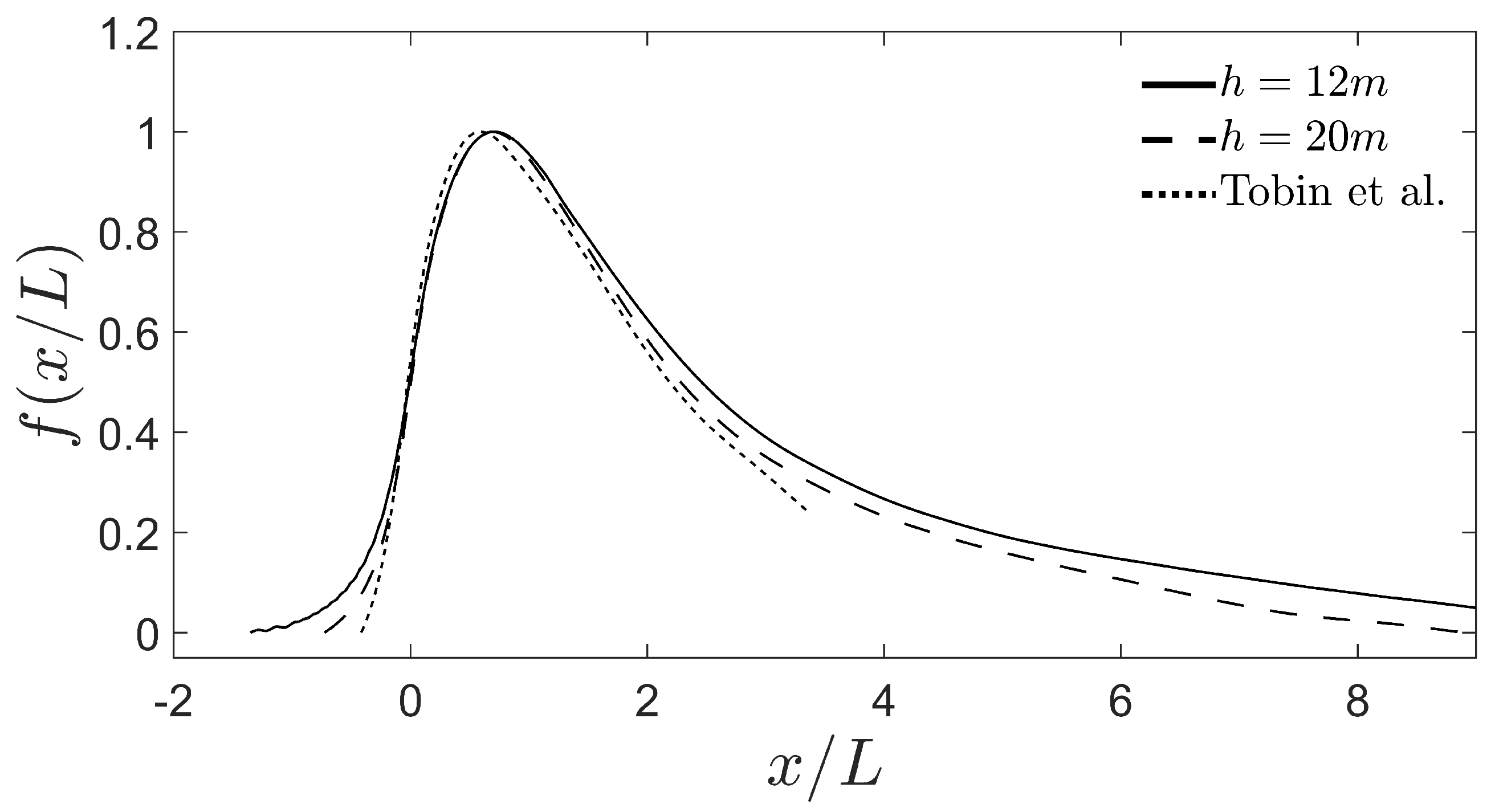
The function is found to agree well with that reported in Tobin et al. [7], as shown in Figure 4. For both the windbreak heights tested, was found to be 9.3 for k = 25. The value as estimated from the LES data is in very good agreement with experiments, while the value is slightly higher. These simulations also allowed for the estimation of the drag coefficient based on the pressure drop across windbreaks and the maximum upwind velocity, with a value of . This value is used in modelling the wind farm flow.
3.2. Power Output Measurements
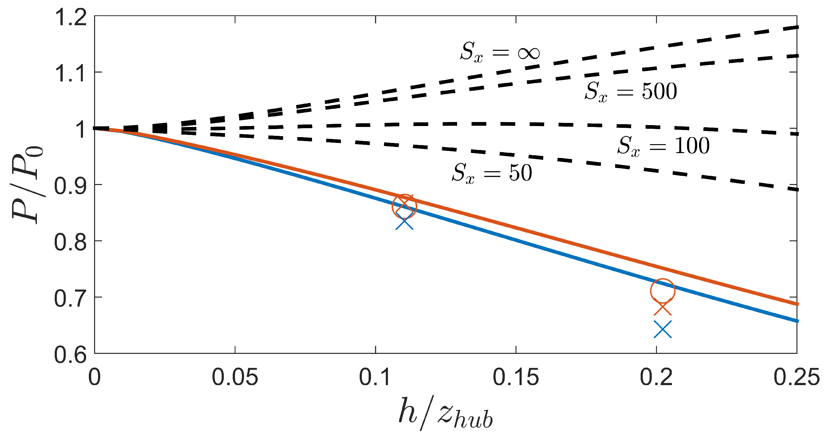
For the inter-turbine spacings tested, predictions suggest that the total impact on power output is negative. This is corroborated with LES data, as shown in Figure 5. Predictions made with boundary-layer theory agree well with data for both the and spacing cases, though they tend to over-predict the data for the larger windbreak. The data do not show a significant difference in the staggered case from the aligned case, though the impact of streamwise spacing is notable, with the case producing less power than either the aligned or staggered case. By extrapolating the top-down theory to greater spacings, it is found that a streamwise inter-turbine spacing on the order of 100 rotor diameters is needed for the positive and negative effects of the windbreaks to balance when , though computational costs prevent the investigation of this wide spacing. If spacing were equal in both the x- and y-directions, this would indicate an inter-turbine spacing of , though this ignores the asymmetry between the effects of streamwise and spanwise spacing.
For a simple two-turbine case with , Tobin et al. [7] showed that the impact of tall windbreaks on downwind turbines is generally negative, though a small benefit was found for shorter ones. The data from the current study are further evidence that windbreaks might not be appropriate for wind farm layouts that have significant wake effects.
3.3. Impact of Porosity
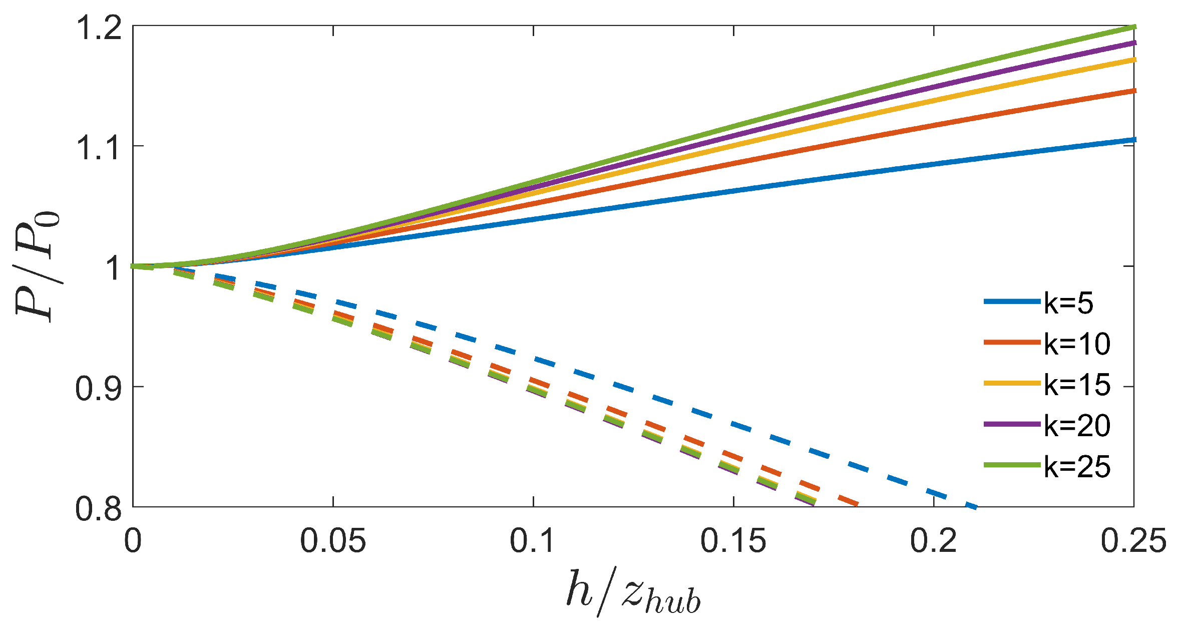
As the pressure coefficient k is reduced, both the inviscid speed-up and the windbreak drag coefficient are diminished. In the limiting case of a single turbine, the most porous windbreak () should be expected to provide only 52% of the power increase of the most porous (). However, this also results in a significant decrease of the windbreak’s drag coefficient from 0.77 to 0.55. The net result of these two impacts for finite inter-turbine spacing is that the magnitude of the change in power is smaller for very porous windbreaks, but the sign of that change is generally the same for a given inter-turbine spacing. This effect is shown in the predicted power perturbations for the porosities tested in Figure 6, though no wind-farm cases were simulated.
3.4. Boundary-Layer Predictions
By augmenting the wake-enhanced approach of Calaf et al. [10] with the roughness predictions of Arya [11], good predictions are made for both the surface shear stress and the roughness length above the wind farm, as shown in Figure 7. Estimation of the middle-layer aerodynamic quantities and is complicated by the fact that both need to be estimated and are not constrained by the prescribed quantities and . The middle quantities are therefore not reported. However, in the bottom and top layers, and are easily measured by fitting a logarithmic velocity profile to the data.
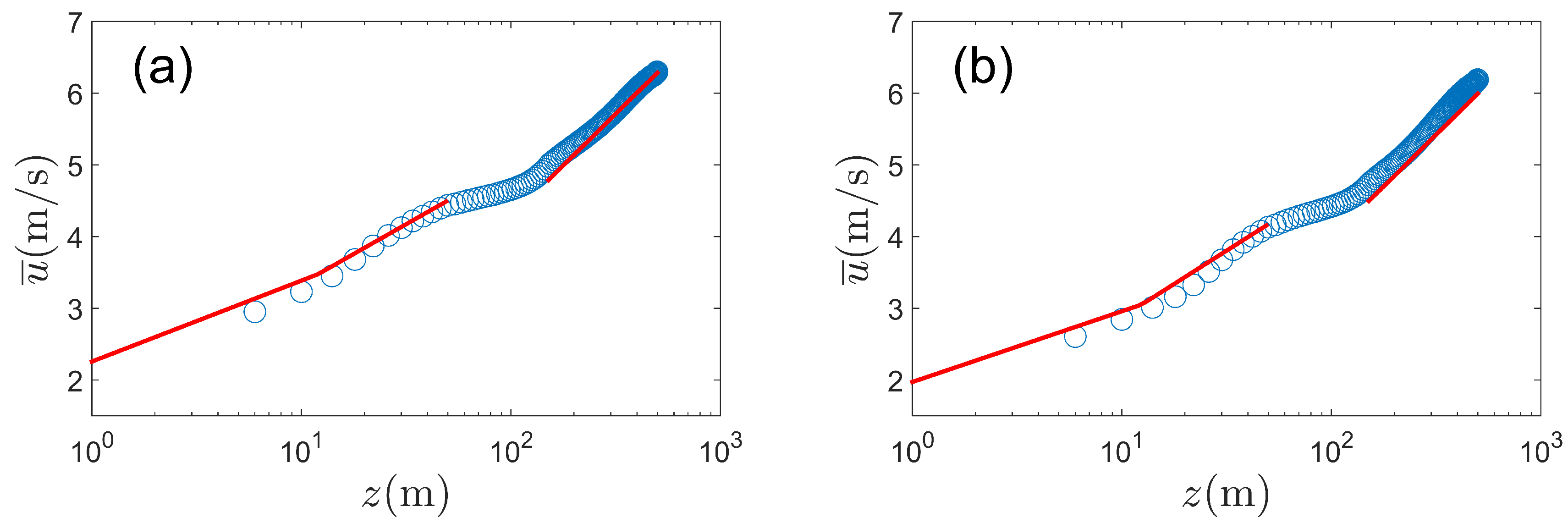
The boundary layer model tends to over-predict the surface shear, which is likely the source for the over-prediction of power output, as is proportional to surface shear. This would then impact the prediction of the wind speed approaching the windbreak, affecting the predicted inviscid speed-up. Although the middle quantities and are not reported from the data, the logarithmic region is a very good fit for the data in the heights between windbreak and the bottom tip of the turbine, as shown in Figure 8 in the case.
4. Conclusions
The suitability of windbreaks for enhancing the power output of a large wind farm was investigated using simplified formulations. Predictions based on the top-down model of wind farm boundary layers combined with an inviscid speedup agree well with LES data, and show that the impact of windbreak wakes is greater than the benefit of their inviscid speedup for infinite wind farms with realistic inter-turbine spacing, suggesting that this approach is not effective for large wind farms. Very wide inter-turbine spacings are required to achieve a positive effect. Results suggest that the porosity of the windbreak does not generally affect whether the change in power is positive or negative, but only affects the magnitude of the change. Therefore, it is not expected that very porous windbreaks will provide a benefit over more solid ones for most layouts. Future work will then need to focus on the development of a more general wake modeling approach for windbreaks, and identifying cases where windbreaks can be used effectively—for instance, in the last row of a wind farm, or in layouts where wake effects are minimal.
Acknowledgments
This material is based upon work supported by the National Science Foundation Graduate Research Fellowship Program under Grant Number DGE-1144245. This work was supported by the Department of Mechanical Science and Engineering, University of Illinois at Urbana-Champaign, as part of the start-up package of Leonardo P. Chamorro. This work used the Extreme Science and Engineering Discovery Environment (XSEDE), which is supported by National Science Foundation grant number OCI-1053575. Specifically, it used the Bridges system, which is supported by NSF award number ACI-1445606, at the Pittsburgh Supercomputing Center (PSC).
Author Contributions
Nicolas Tobin prepared and ran the simulations, and prepared the manuscript. Leonardo P. Chamorro contributed to the preparation of the manuscript.
Conflicts of Interest
The authors declare no conflict of interest.
References
- Chamorro, L.P.; Arndt, R.E.A.; Sotiropoulos, F. Turbulent flow properties around a staggered wind farm. Bound.-Layer Meteorol. 2011, 141, 349–367. [Google Scholar] [CrossRef]
- Meyers, J.; Meneveau, C. Optimal turbine spacing in fully developed wind farm boundary layers. Wind Energy 2012, 15, 305–317. [Google Scholar] [CrossRef]
- Palma, J.M.L.M.; Castro, F.A.; Ribeiro, L.F.; Rodrigues, A.H.; Pinto, A.P. Linear and nonlinear models in wind resource assessment and wind turbine micro-siting in complex terrain. J. Wind Eng. Ind. Aerodyn. 2008, 96, 2308–2326. [Google Scholar] [CrossRef]
- Chamorro, L.P.; Tobin, N.; Arndt, R.E.A.; Sotiropoulos, F. Variable-sized wind turbines are a possibility for wind farm optimization. Wind Energy 2014, 17, 1483–1494. [Google Scholar] [CrossRef]
- Fleming, P.A.; Gebraad, P.M.O.; Lee, S.; van Wingerden, J.W.; Johnson, K.; Churchfield, M.; Michalakes, J.; Spalart, P.; Moriarty, P. Evaluating techniques for redirecting turbine wakes using SOWFA. Renew. Energy 2014, 70, 211–218. [Google Scholar] [CrossRef]
- Xie, S.; Archer, C.L.; Ghaisas, N.; Meneveau, C. Benefits of collocating vertical-axis and horizontal-axis wind turbines in large wind farms. Wind Energy 2017, 20, 45–62. [Google Scholar] [CrossRef]
- Tobin, N.; Hamed, A.M.; Chamorro, L.P. Fractional Flow Speed-Up from Porous Windbreaks for Enhanced Wind-Turbine Power. Bound.-Lay. Meteorol. 2017, 163, 253–271. [Google Scholar] [CrossRef]
- Denholm, P.; Hand, M.; Jackson, M.; Ong, S. Land-Use Requirements of Modern Wind Power Plants in the United States; Technical Report No. NREL/TP-6A2-45834; National Renewable Energy Laboratory: Golden, CO, USA, 2009.
- Frandsen, S. On the wind speed reduction in the center of large clusters of wind turbines. J. Wind Eng. Ind. Aerodyn. 1992, 39, 251–265. [Google Scholar] [CrossRef]
- Calaf, M.; Meneveau, C.; Meyers, J. Large eddy simulation study of fully developed wind-turbine array boundary layers. Phys. Fluids 2010, 22, 015110. [Google Scholar] [CrossRef]
- Arya, S.P.S. A drag partition theory for determining the large-scale roughness parameter and wind stress on the Arctic pack ice. J. Geophys. Res. 1975, 80, 3447–3454. [Google Scholar] [CrossRef]
- Stevens, R.J.A.M.; Gayme, D.F.; Meneveau, C. Coupled wake boundary layer model of wind-farms. J. Renew. Sustain. Energy 2015, 7, 023115. [Google Scholar] [CrossRef]
- Yang, X.; Kang, S.; Sotiropoulos, F. Computational study and modeling of turbine spacing effects in infinite aligned wind farms. Phys. Fluids 2012, 24, 115107. [Google Scholar] [CrossRef]
- Dong, Z.; Luo, W.; Qian, G.; Wang, H. A wind tunnel simulation of the mean velocity fields behind upright porous fences. Agric. For. Meteorol. 2007, 146, 82–93. [Google Scholar] [CrossRef]
- Fang, F.M.; Wang, D.Y. On the flow around a vertical porous fence. J. Wind Eng. Ind. Aerodyn. 1997, 67, 415–424. [Google Scholar] [CrossRef]
- Nystrom, N.A.; Levine, M.J.; Roskies, R.Z.; Scott, J. Bridges: A uniquely flexible HPC resource for new communities and data analytics. In Proceedings of the 2015 XSEDE Conference: Scientific Advancements Enabled by Enhanced Cyberinfrastructure, St. Louis, MO, USA, 26–30 July 2015; ACM: New York, NY, USA, 2015; p. 30. [Google Scholar]
- Towns, J.; Cockerill, T.; Dahan, M.; Foster, I.; Gaither, K.; Grimshaw, A.; Hazlewood, V.; Lathrop, S.; Lifka, D.; Peterson, G.D.; et al. XSEDE: Accelerating scientific discovery. Comput. Sci. Eng. 2014, 16, 62–74. [Google Scholar] [CrossRef]
- Smagorinsky, J. General circulation experiments with the primitive equations: I. The basic experiment. Mon. Weather Rev. 1963, 91, 99–164. [Google Scholar] [CrossRef]
- van Driest, E.R. On Turbulent Flow Near a Wall. J. Aeronaut. Sci. 1956, 23, 1007–1011. [Google Scholar] [CrossRef]
- Laws, E.M.; Livesey, J.L. Flow through screens. Annu. Rev. Fluid Mech. 1978, 10, 247–266. [Google Scholar] [CrossRef]
- Raupach, M.R.; Woods, N.; Dorr, G.; Leys, J.F.; Cleugh, H.A. The entrapment of particles by windbreaks. Atmos. Environ. 2001, 35, 3373–3383. [Google Scholar] [CrossRef]
- Counihan, J.; Hunt, J.C.R.; Jackson, P.S. Wakes behind two-dimensional surface obstacles in turbulent boundary layers. J. Fluid Mech. 1974, 64, 529–564. [Google Scholar] [CrossRef]
Figure 1.
Conceptual schematic of the layout of an infinite wind farm with windbreaks. Dashed lines show the region with reversed flow.
Figure 1.
Conceptual schematic of the layout of an infinite wind farm with windbreaks. Dashed lines show the region with reversed flow.
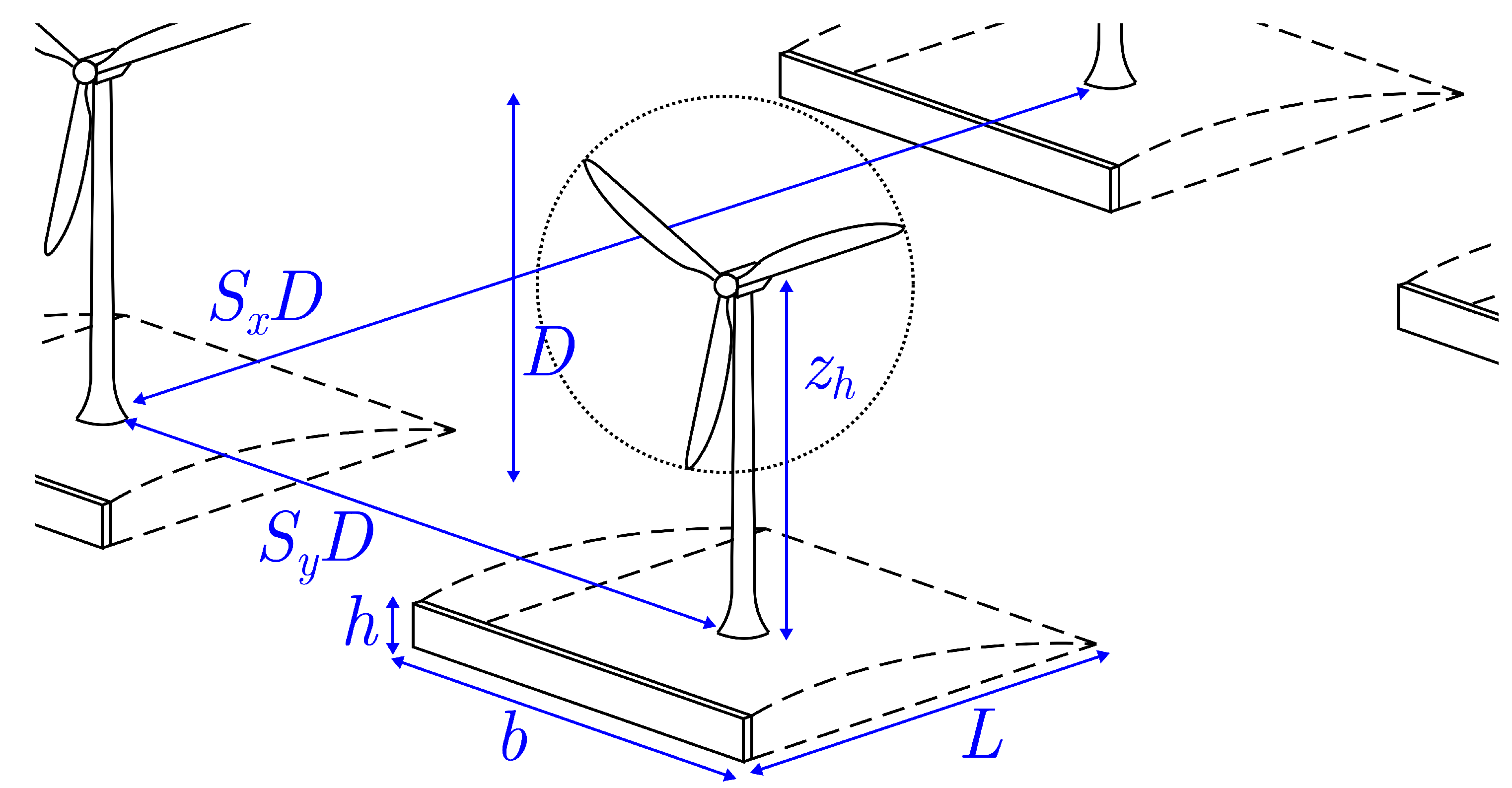
Figure 2.
The several flow regions with their respective aerodynamic properties.

Figure 3.
(a) Averaged boundary-layer profile with no turbines or windbreaks present. Blue markers indicate LES data, and red lines indicate a logarithmic boundary-layer profile; (b) Velocity power spectrum simulated at turbine hub height.
Figure 3.
(a) Averaged boundary-layer profile with no turbines or windbreaks present. Blue markers indicate LES data, and red lines indicate a logarithmic boundary-layer profile; (b) Velocity power spectrum simulated at turbine hub height.
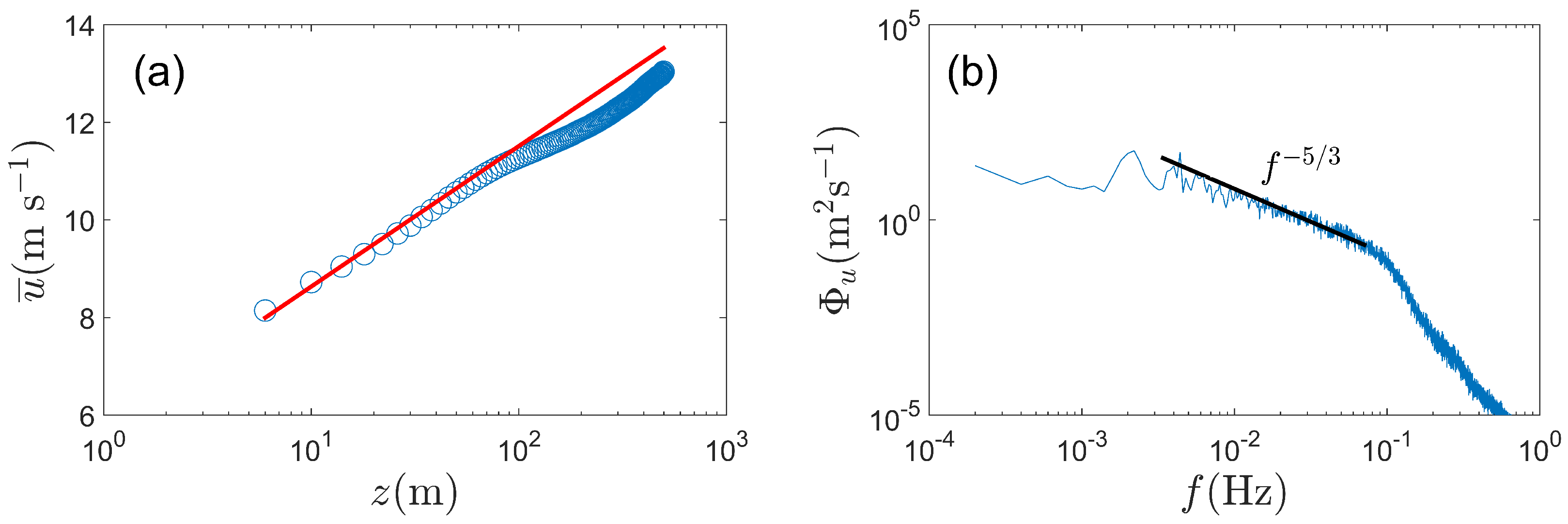
Figure 4.
The function from the current simulations for and from Tobin et al. [7].
Figure 4.
The function from the current simulations for and from Tobin et al. [7].

Figure 5.
Power output predictions based on the top-down model along with LES data. Blue markers indicate , and red counterparts denote ; ×s indicate aligned arrangement, and circles indicate staggered wind farm.
Figure 5.
Power output predictions based on the top-down model along with LES data. Blue markers indicate , and red counterparts denote ; ×s indicate aligned arrangement, and circles indicate staggered wind farm.

Figure 6.
Power output predictions for several windbreak porosities based on the top-down model along with LES data. Solid lines indicate , and dashed lines indicate .
Figure 6.
Power output predictions for several windbreak porosities based on the top-down model along with LES data. Solid lines indicate , and dashed lines indicate .

Figure 7.
(a) Predicted versus simulated aerodynamic properties for an infinite wind farm: surface shear stress; (b) Aerodynamic roughness length. Blue markers indicate , and red markers indicate ; ×s indicate an aligned arrangement, and circles indicate staggered.
Figure 7.
(a) Predicted versus simulated aerodynamic properties for an infinite wind farm: surface shear stress; (b) Aerodynamic roughness length. Blue markers indicate , and red markers indicate ; ×s indicate an aligned arrangement, and circles indicate staggered.
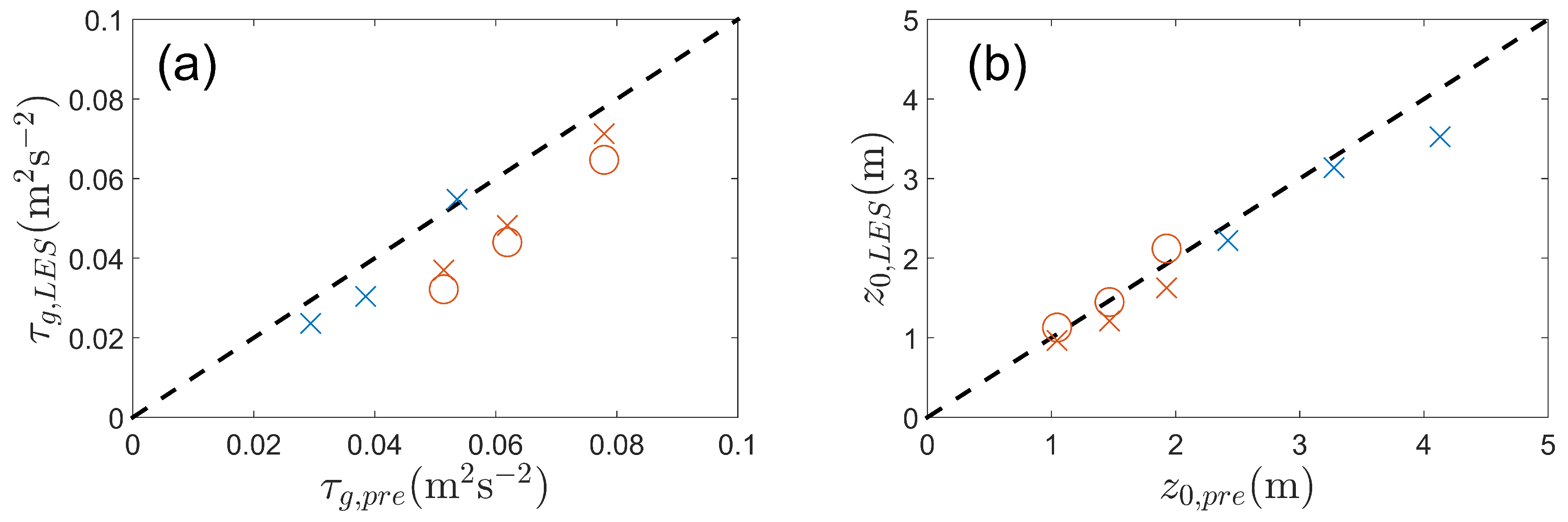
Figure 8.
Predicted and simulated areally averaged boundary-layer velocity profiles for an infinite wind farm showing distinct logarithmic regions: (a) , m; (b) , m. Blue markers indicate LES data, and red lines indicate boundary-layer predictions.
Figure 8.
Predicted and simulated areally averaged boundary-layer velocity profiles for an infinite wind farm showing distinct logarithmic regions: (a) , m; (b) , m. Blue markers indicate LES data, and red lines indicate boundary-layer predictions.

Table 1.
Windbreak and wind farm cases inspected with large-eddy simulations.
| h (m) | No. of Turbines | Alignment | k | (m) (m) (m) | ||
|---|---|---|---|---|---|---|
| 6 | 5 | 0 | Aligned | 25 | ||
| 6 | 5 | 12 | Aligned | 25 | ||
| 6 | 5 | 20 | Aligned | 25 | ||
| 10 | 5 | 0 | Aligned | 25 | ||
| 10 | 5 | 12 | Aligned | 25 | ||
| 10 | 5 | 2 | Aligned | 25 | ||
| 10 | 5 | 0 | Staggered | 25 | ||
| 10 | 5 | 12 | Staggered | 25 | ||
| - | - | 12 | - | - | 25 | |
| - | - | 20 | - | - | 25 | |
| - | - | 12 | - | - | 20 | |
| - | - | 12 | - | - | 15 | |
| - | - | 12 | - | - | 10 | |
| - | - | 12 | - | - | 5 |
© 2017 by the authors. Licensee MDPI, Basel, Switzerland. This article is an open access article distributed under the terms and conditions of the Creative Commons Attribution (CC BY) license (http://creativecommons.org/licenses/by/4.0/).
Share and Cite
MDPI and ACS Style
Tobin, N.; Chamorro, L.P. Windbreak Effects Within Infinite Wind Farms. Energies 2017, 10, 1140. https://doi.org/10.3390/en10081140
AMA Style
Tobin N, Chamorro LP. Windbreak Effects Within Infinite Wind Farms. Energies. 2017; 10(8):1140. https://doi.org/10.3390/en10081140
Chicago/Turabian StyleTobin, Nicolas, and Leonardo P. Chamorro. 2017. "Windbreak Effects Within Infinite Wind Farms" Energies 10, no. 8: 1140. https://doi.org/10.3390/en10081140
Note that from the first issue of 2016, this journal uses article numbers instead of page numbers. See further details here.