A Simplified Microgrid Model for the Validation of Islanded Control Logics
by
 , ,
, ,
Andrea Bonfiglio
* ,
,
Massimo Brignone
 ,
,
Marco Invernizzi
, 
Alessandro Labella
, 
Daniele Mestriner
and 
Renato Procopio

DITEN Department of Electrical, Electronic, TLC Engineering and Naval Architecture, University of Genoa, 16145 Genoa, Italy
*
Author to whom correspondence should be addressed.
Energies 2017, 10(8), 1141; https://doi.org/10.3390/en10081141
Submission received: 19 June 2017
/
Revised: 25 July 2017
/
Accepted: 30 July 2017
/
Published: 3 August 2017
Abstract
:Microgrids (MGs) may represent a solution in the near future to many problems in the energy and electric world scenarios; such as pollution, high reliability, efficiency and so on. In particular, MGs’ capability to work in an islanded configuration represents one of their most interesting features in terms of the improvement of the reliability of the system, the integration of renewable energy sources and the exploitation of the quick response and flexibility of power electronic devices in a stand-alone system. In order to study and validate innovative solutions and control strategies for islanded operation, there is a need to develop models for MG structures that can be reliable and sufficiently simple to be used for the purpose of the design and validation of innovative control systems. This paper proposes a simplified, first harmonic model for a generic structure of MG characterized by its use of only electronic power converter interfaced generation. The main advantages of the proposed method lie in the model’s simplicity and its reduced solving time, thanks to the limited number of necessary parameters to describe the system. Moreover, the developed formulation allows the avoidance of specific (and often licensed) software to simulate the system. The performances of the proposed model have been validated by means of a comparative analysis of the results obtained against a more accurate representation of the system performed in the power system CAD—electromagnetic transient and DC (PSCAD—EMTDC) environment, which allows for the representation of each component with a very high level of detail. Such comparison has been performed using the University of Genoa Savona Campus Smart Polygeneration Microgrid testbed facility, due to the availability of all the necessary numerical values.
1. Introduction
The development of renewable energy sources (RESs) and of distributed energy resources (DERs), aimed at the reaching of a reduction in greenhouse gas emissions, has led to a massive growth of microgrid (MG) studies and actual realizations [1,2,3]. The integration of RES is one of the most important and challenging aspects that researchers are facing in order to obtain a stable and reliable operation of the power grid, as the increasing number of wind and photovoltaic power plants is decreasing the inertia of the power system [4,5,6]. MGs can easily integrate RES into the electric network, guaranteeing an optimized management, both from the economic and the environmental point of view, and a higher level of power quality [7,8]. Moreover, if an MG is capable of working in an islanded configuration and to seamlessly transit from an islanded to grid-connected form, and vice-versa, this could generate a scenario where the power system is capable of modulating itself in accordance to the need of having a stable asset using MG capabilities to modulate the balance between load and generation. Due to their complexity and the variety of their sources and infrastructures, MGs also represent one of the best environments for the testing of innovative and advanced control and energy management systems. In this framework, the necessity for a reliable model of an MG is essential in order to use it for control system design, the tuning of its parameters and the validation of innovative energy management logics. This goal can be reached, in one way, by representing the MG in an electromagnetic power system simulator (e.g., power system CAD—electromagnetic transient and DC (PSCAD—EMTDC) [9], SPICE (simulation program with integrated circuit emphasis) [10], PLECS (piecewise linear electrical circuit simulation) [11]). The advantage of this approach is that the resulting model is extremely detailed; on the other hand, (i) it requires a lot of time set up the model; (ii) trained users are required and (iii) each simulation becomes very cumbersome from a CPU point of view. It is well known that any model introduces approximations and has a domain of validity. The value of a model is represented by the tradeoff between reliability, accuracy and simplicity: in particular, this last characteristic is very important for the reduction of computational effort and to give the users the possibility to handle the model easily and to have a sensitivity regarding the way variables interact with each other. Indeed, another possible approach is to develop a simplified model that is able to describe all the phenomena that must be taken into account when designing a proper control system suited for a specific MG. Simplified equivalent models are very strong instruments for analyzing MG behavior; an overview on these models is presented in [12,13]. One of the most commonly-used approximations consists of neglecting the voltage drop along the connection (i.e., the so-called single bus bar (SBB) model, according to which generators and loads are positioned at the same bus [14,15,16]). In other works [17,18,19], in order to evaluate the power flow easily, voltages are considered equal to one per unit so that it is possible to mismatch current with apparent power. Moreover, in [20] a simplified ordinary differential equations (ODEs) system to evaluate MG behavior is presented; for economic purposes only.
The most relevant part of the bibliography deals with the developing of MG models in the view of energy management systems accounting for longer time horizons (several seconds, hours, days), in order to manage power sharing and the stochastic behavior of loads and renewables [21,22,23,24]. The amount of the literature is considerably reduced if one considers islanded microgrids, especially those characterized by no synchronous generators connecting directly to the main AC system. In this configuration, the issue of frequency and voltage control and load sharing is more difficult and cannot rely on the scheme adopted for traditional regulation. For this reason, a simplified way of representing the dynamic behavior of a MG characterized by only power electronic interfaced generation would represent a useful tool to study and test innovative control strategies for islanded MGs.
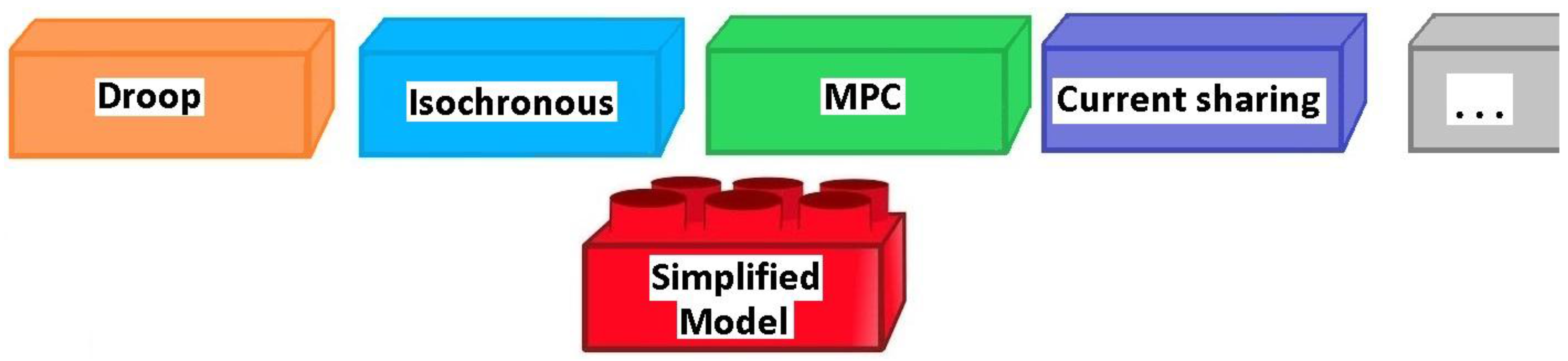
The present paper aims at developing a simplified model that accounts for all the details typical of a fundamental frequency analysis and is able to handle and to evaluate all the voltage and frequency transients necessary to test a primary regulation scheme. As will be clarified later in the paper, contrary to the SBB approximation, the methodology proposed in this paper does not neglect voltage deviations and/or power losses [16,17,18,19,20,25] and allows one to perform a complete analysis of the evolution of all the electric variables. The proposed approach results in a system of ODEs that can be implemented in any general purpose software, opening the possibility of interfacing it with both traditional MG control systems [26,27,28,29] and more advanced ones [30,31,32] and allowing it to account both for islanded and grid-connected configurations. In other words, the challenge of the proposed model, which represents an optimal trade-off between accuracy and simplicity, is that it can be used as a universal general MG emulator, just like a base brick compatible with many lids, representing the control logics (Figure 1). These lids can be elementary, as droop [27], isochronous [33] and current sharing [34], but also based on complex and advanced optimization and control algorithms (e.g., model predictive control (MPC) [35,36,37] and feedback linearization (FBL) [38]). In conclusion, the advantages of the proposed model can be summarized as follows:
- (a)
- Provide a simple but reliable model for islanded MGs, characterized by all the generation interfaced to the AC part of the MG by means of power electronic devices;
- (b)
- Running the model does not require a dedicated, often licensed, specific software, a relevant time to set up the model and a high computational effort;
- (c)
- The model is presented as a system of ODE that does not need too many input parameters and can be used to design different controllers and tune their parameters.
The proposed model has been validated comparing its results with the ones provided by PSCAD—EMTDC on the Smart Polygeneration Microgrid (SPM) of the Savona Campus of Genoa University [39], highlighting a very good agreement between the two simulators.
The paper is organized as follows: Section 2 briefly presents the SPM layout while Section 3 describes its main elements; Section 4 derives the simplified model, highlighting the main assumptions it relies upon. Section 5 recalls the principles of two control strategies, which are used as an example to show the interfacing between the developed power system model and the controller equations. Section 6 presents the power system CAD (PSCAD) environment SPM complete model used to validate the proposed approach and the simulation results. Finally, in Section 7 some conclusions about the work are drawn.
2. The Savona Campus Smart Polygeneration Microgrid
The SPM is a tri-generative, low voltage (LV) MG realized in the Savona Campus of Genoa University, in operation since February 2014. The SPM is an infrastructure realized for demonstrative and research purposes and is intended as a test-bed facility for innovative solutions for MG management and control. In order to achieve this goal, the SPM accounts for various types of generations (tri-generative micro-turbine, photovoltaic and concentrating solar power units), storage devices, electric vehicle charging stations, thermal production units and the campus as an electric and thermal load. The SPM project now represents an important research area for the validation of new algorithms, logics and management strategies to provide and improve innovative solutions to the problem of the integration of DERs and energy storages; fundamental requirements, for example, to the European 20-20-20 calls (Horizon 2020 Programme for Research) [40]. In 2017, a portion of SPM is being tested in an islanded configuration and analyzed in terms of stability and load sharing. This portion is represented in Figure 2 and consists of:
- The public grid connected to a switchgear (SG) Q1;
- Three photovoltaic (PV) units connected through a unique cable to the SG Q1, namely PV1;
- One PV unit (with its inverter and transformer) connected to SG Q2, namely PV2;
- The storage unit produced by FIAMM (with its DC/DC converter, inverter and transformer) connected to SG Q2;
- Resistive-inductive loads connected to SG Q2.
The sources, ratings, and the main data of the network components are reported in Table 1.
Moreover, both PV2 and the storage have a transformer, whose rated values are 80 kVA, 6%, 200/400 V and 70 kVA, 4%, 400/400 V respectively.
3. MG Sources and Main Elements
In the present section, a mathematical modeling of the SPM components involved in the islanded portion is presented.
3.1. PV Units Model
The PV modules are modeled as DC dipoles whose voltage–current characteristic curve (dependent on the irradiance α in W/m2, the temperature T in °C and the V voltage expressed in V) in the I–V plane is described as follows [41]:
where the meaning of symbols and their values are reported in Table 2. The number p of parallel modules and s of series modules is: p = 3 and s = 22 for PV1 and p = 14 and s = 24 for PV2.
3.2. Electric Storage Model
The electric storage system is a FIAMM SoNick battery (Zebra), with a rated capacity of 141 kWh, 228 Ah of nominal current capacity (NCC), a rated power of 62 kW when suppling and 30 kW when absorbing. It is structured in Nm = 6 modules in parallel, each one composed by the series of Nc = 240 cells [42]. The storage is represented by a non-ideal DC voltage generator, where the produced voltage V is a function of its state of charge (SOC) [43], its internal resistance Rint and the current I injected by the storage, according to the following equation:
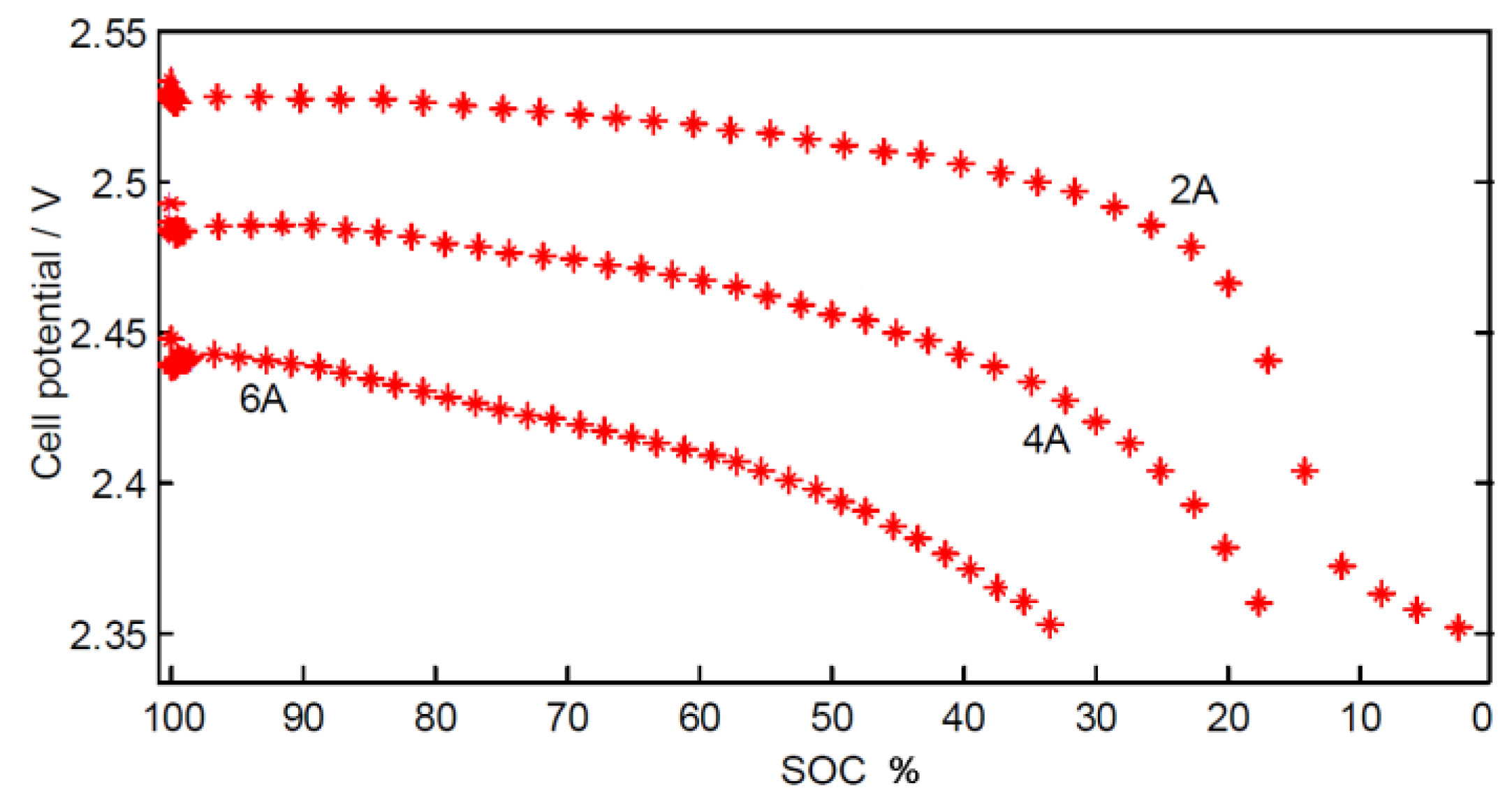
where the internal voltage (E) is an unknown function of the SOC, to be deduced from measured data. The model proposed in (2) is justified observing Figure 3, where it can be noticed that discharging the battery at different (constant) currents results in a rigid translation of the curve. Under this assumption, for a fixed value of the SOC, the voltage V depends proportionally on the current. In terms of an electric equivalent, if there is a linear relationship between voltage and current, there is an internal resistance whose value can be estimated by simply knowing two voltage-current couples.
For each current I, a set of N measurements is available in Figure 3, formally encoded in the following:
where, for our measurements, NI = 3 and I1 = 2 A, I2 = 4 A and I3 = 6 A. The cell resistance value can be calculated as the following average:
which allows us to find that Rcell = 0.028 Ω. As a consequence, the pairs (SOCk, Ecell,k) can be obtained as follows:
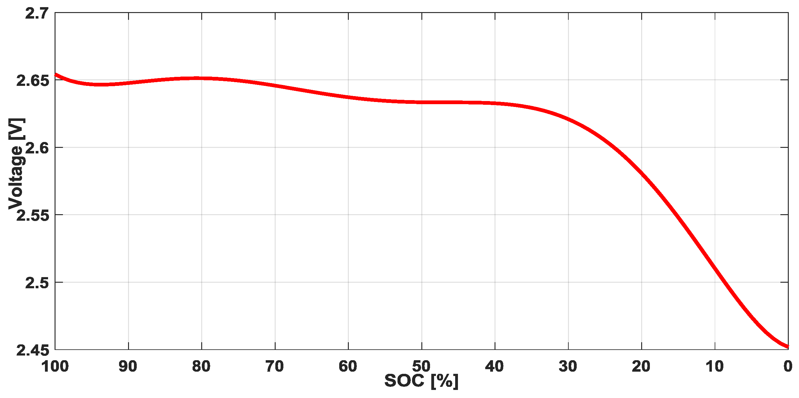
Finally the possible analytical expression for the link between the internal voltage and the SOC can be obtained fitting the pairs (SOCk, Ecell,k) with the following polynomial formula:
where the coefficients ai have been found with a least-square method aimed at minimizing the difference between the polynomial output and the measured sequence Ecell,k. The numerical values of the coefficients are reported in Table 3 and the resulting curve is depicted in Figure 4.
Then, the results for the maximum voltage of a single cell are:
therefore, the maximum voltage of the overall storage is:
and the internal resistance is:
The dependence of the voltage on the temperature is neglected according to Zebra features [44]. Often, and therefore also in this MG, a DC/DC bidirectional converter is interposed between the storage and its inverter (this will be discussed in detailed in the following).
3.3. Inverter Model
The aim of the inverter is to couple the DC sources to the AC grid correctly. Each inverter is modeled by the mean-values input/output relation, thus:
where is voltage phasor, m is the modulation index, VDC is the voltage at DC terminals, j, as usual, is the imaginary unit, and δ is the angle of the phasor.
3.4. DC/DC Converter Model
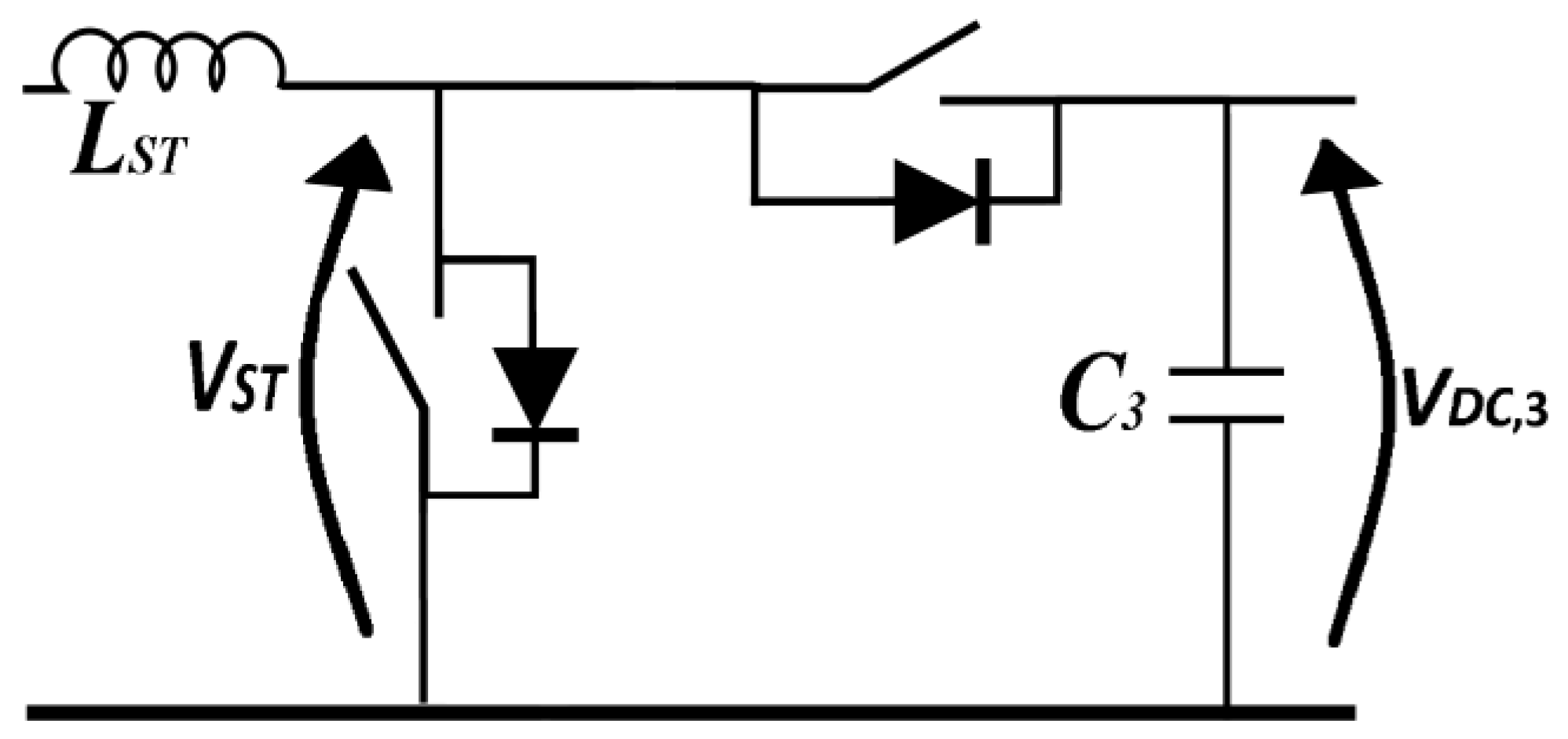
In order to allow for the proper operation of the inverter, it is necessary to keep its DC voltage as constant as possible. Thanks to the MPPT (maximum power point tracker) algorithm, PV inverters are controlled in a way that keep the DC voltage almost constant, as the MPP (maximum power point) voltages do not vary by very much [45]. The storage inverters, on the other hand, are characterized by a sensitive variation of the voltage on the battery; thus, they need a dedicated control of the voltage obtained by the insertion of a DC/DC bi-directional (buck-boost) chopper. The DC/DC converter has the structure depicted in Figure 6 [46].
The well-known chopper input/output relationship [46] is given by:
being VDC,3 and VST the DC/DC output (inverter side) and input (battery side) voltages respectively, while KST is related to the switch duty cycles D1 (boost) and D2 (buck) according to the following:
being PST the power injected by the storage into the network. Moreover, a filter consisting of a series inductor and a shunt capacitor have been inserted, whose values are 1 mH and 0.5 mF respectively.
4. The Simplified Model
The aim of this work is to find an approximate model able to adequately represent both the transient and the steady state of any MG, after a contingency. To do this, the following simplifications are introduced:
- Each input/output power electronic converter relationship neglects the presence of the higher order harmonics;
- The shunt sections of the inverter AC filters are neglected for simplicity (indeed it can be noted from Table 3 that the shunt filter impedance at the fundamental frequency is more than 3 kΩ). If one considered this, it would imply only an enlargement of the network admittance matrix Y without changing the model structure;
- The AC-side portion of the MG (as well as the inverter filter) is supposed to be at a steady state (assuming that both the angular frequency of the sources and their voltage amplitude can vary), while all the DC dynamics are accounted;
- The loads are described with a constant impedance model. Consequently, as typical in RMS transients, they are inserted in the network model, giving rise to the so-called extended admittance matrix YE [47].
Thus, in the case of the SPM, the portion described in Figure 2 collapses in the one shown in Figure 7. As will be clear in writing the equations, it is apparent that the description of the AC grid with the extended admittance matrix allows for a coupling of the source dynamics in a simple but effective way.
The first assumption allows us to write that [46]:
where j, as usual, is the imaginary unit, and, for the k-th source, mk is the modulation index (in accordance to its linear meaning [46], it lies in the range (0, 1.15)) and δk is the angle such that:
where
while ωk and φk are the angular frequency and the phase of the k-th source, respectively. The main network is an independent voltage source, whose phasor is given by:
Thus, the active power injected by the k-th source (k = 1, 2, 3) is given by:
where YE,ki = Gki + jBki is the (k, i) element of the extended admittance matrix. As stated before, Equation (17) shows the strong coupling of the sources through YE. Moreover, for each PV capacitor, the power balance can be written as:
while the storage capacitor power balance results in:
Inserting (14) into (17), then (17) into (18) and (19), one finally gets the system of ordinary differential Equations (15) and (18)–(21), which completely describes the DC dynamics, and so the complete dynamics of the MG under the aforementioned assumptions. A differential equations (ODE) system can be written as:
where f collects (15) and (18)–(21), while the vectors X and U are given by:
The initial equilibrium point can be obtained by solving the non-linear algebraic system, obtained by zeroing all the time derivatives in (22).
Starting from an assigned equilibrium point, a structure perturbation (encoded in a variation in one or more elements of the extended admittance matrix) causes the dynamics. It is useful to underline that, in order to exclude a source from the analysed grid, it is sufficient to cancel the related admittances, highlighting the flexibility of the proposed approach to be applied at different MG structures. It is important to highlight that U is the input vector used to create the modulating signal of the PWM (pulse-width modulation) to control the AC voltage of each inverter: amplitude (m), frequency (ω) and phase (φ).
In conclusion, a step by step synopsis could be useful to summarize the whole procedure:
- Define the MG topology, parameters (rated data of cables, transformers, sources etc.) and admittance matrix;
- Define the sources and their characteristic (power–irradiance for PV, power-wind velocity for wind generator, V-SOC for chemical storage etc.);
- Define the all the state variables and write the resulting ODEs;
- Define an equilibrium point of the system zeroing all of the time derivatives;
- Define a contingency;
- Solve the resulting ODE system and get the involved variable dynamics.
5. Controllers
One of the aims of the paper is to show that the developed model can be adopted to design suitable MG controllers, set up their parameters and test their performances. To do this, in the present section, after a brief overview of the control system for the DC/DC converter (Section 5.1), two control examples are described; namely, the droop-based control (quickly recalled in Section 5.2) and the isochronous control (summarized in Section 5.3).
5.1. DC/DC Converter Controller
The DC/DC converter control logic is explained by (24) and (25), where the sign of the power produced by the storage in AC side (PST) activates either the buck or the boost level control. Both of them consist of PI (proportional integral) regulators that implement the following equations:
being
Thus, χ1 and χ2 represent the state of the two different PI controllers.
The chosen proportional gains and integral time constants appear in Table 5. The whole system being strongly non-linear, the usual tuning techniques lack validity; thus, here and in the following the PI parameters are chosen in a heuristic way to get the best performance in terms of system stability and transient/steady state behavior.
5.2. Droop Control
The droop control, first proposed by M. C. Chandorkar in 1993 [27], is a technique that allows the sharing the load power among different sources without the need for any communication device. Details on the method can be found in [15,48,49]; here, the main controller equations are reported and then connected to those describing the power system model.
where mDk (nDk) is a negative coefficient that represents the slope of the P-ω (Q-V) droop characteristic of the k-th inverter; PAC,k0 (Qk0) is the reference of the active (reactive) power of the machine; PAC,k (Qk) is the actual active (reactive) power produced by the k-th source; Vk0 is the k-th inverter AC side voltage (reference) and ω0 is the rated angular frequency of the MG. In order to ensure a proper load sharing among the sources, mDk and nDk are chosen according to the rated active and reactive power (PiN and QiN) respectively [27,28] thus:
Equation (28) states that, whatever the number of sources in the MG, just one droop coefficient for the active power channel, and only one for the reactive one, can be chosen independently. Inserting (17) into (26), one has:
As pointed out in [27], the droop control does not act on the initial phase φk, which is locked to its initial value. So, inserting (29) into (18), one has:
Moreover, combining the k-th inverter reactive power expression with (27), one has:
which produces the following differential-algebraic equations (DAEs) system:
in which the vector of the states XD is given by:
and U is the vector that contains Vk0 and ω0. Figure 8 shows the strong relation between the control logic and the simplified model, as the input of the power system are the output of the control system and the input of the control systems are the measured and feed-backed power system results.
The function fD appearing in (32) consists of (18)–(21), (25) and (30), having expressed KST as a function of the state variables using (12) and (24), while gD collects (31).
5.3. Isochronous (Master/Slave) Control
The main goal of the isochronous control is to allow the PV sources (slaves) to supply their maximum power [33,50,51], controlling them in the so-called PQ (active and reactive power) control mode [29]. In this way, each load variation will be handled completely by the storage system that acts as a master.
Therefore, one controls the storage system such that it acts as a fixed voltage source, while the PV units are managed by two PI controllers. One receives, as an input, the DC voltage error and produces the phase angle δk as an output of the modulating signals for the PV inverter, while the other processes the reactive power error in order to provide the PWM logic with a suitable modulating index request mk (see [52] for details). It should be noted that the isochronous logic does not act on the angular frequencies ωk, which remain locked in to their rated value. The controllers structure is a specified in (34) and (35), while their parameters appear in Table 6.
The master/slave control produces the following ODE system:
in which the vector of the states X is given by:
the input vector U contains the reference signals for the PV active and reactive power production and fI collects (18)–(22), (25) and (34). Figure 9 shows the relation between the control logic and the simplified model.
6. Simulations
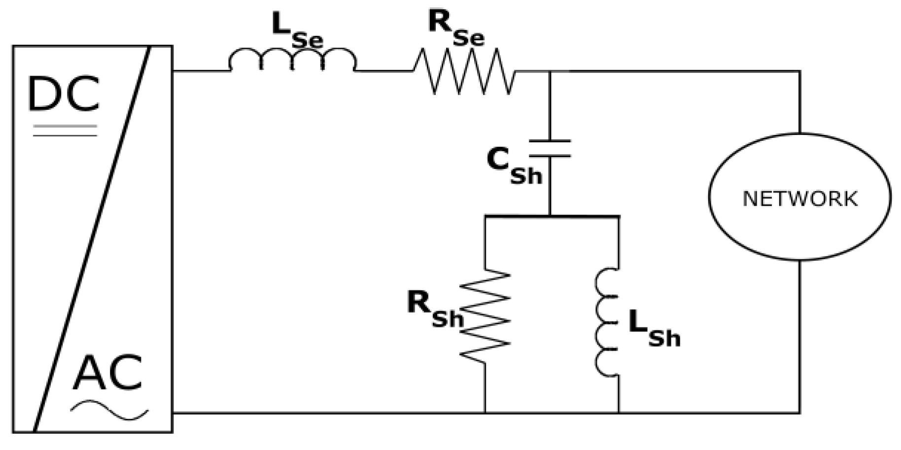
In order to validate the proposed simplified approach, a complete model of the islanded section of the SPM has been set up in the PSCAD-EMTDC environment that allows us to represent all the devices with a high degree of detail. In particular, all the inverters are built with a total controlled bridge of a not-ideal IGBT (insulated gate bipolar transistor), modulated with a PWM technique and equipped with AC filters whose topology appears in Figure 5 using the parameters available in Table 3 [53], considering both the series and the shunt parts. Moreover, the DC/DC converter is an inverter branch modulated through a comparison between a triangle carrier and a reference constant signal [46]. Thus, the whole harmonic spectrum is accounted both at the DC side and at the AC one, contrary to what is done in the simplified model. Finally, the sources are implemented with the same equations used in the simplified model, while the whole infrastructure, being modelled in an electromagnetic environment, accounts both for AC and DC dynamics. A PSCAD view of the complete model is shown in Figure 10.
Two groups of simulations will be presented with two main aims:
- Validating the developed simplified model comparing its results with the ones provided by the complete model implemented in PSCAD-EMTDC;
- Assessing the possibility of interfacing the developed power system model with different controller structures. This will be done considering the two control logics summarized in the previous sections (droop and isochronous).
6.1. Droop Control Simulations
In the following paragraphs, two simulations will be presented; the first one (S1) is characterized by a step decrease in the load resistance with a consequent increase in its active power request, while, in the second one (S2), the load resistance increases resulting in a decrease in its active power absorption. The values of the droop coefficients chosen for both simulations are reported in Table 7.
6.1.1. Active Power Increasing Simulation (S1)
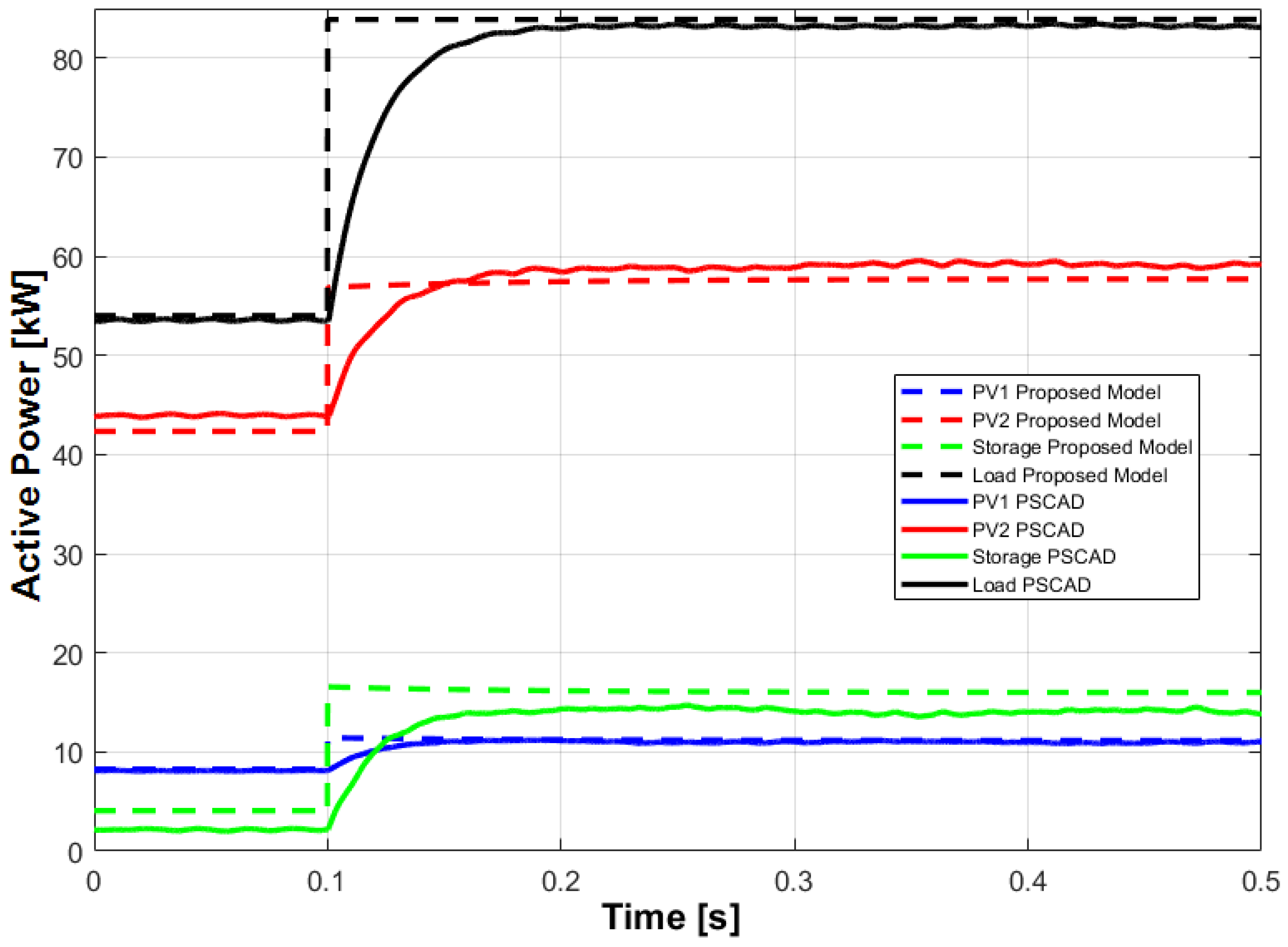
The initial working point is described in Table 8. The contingency occurs at 0.1 s and consists of a step change in the load resistance from 3 Ω to 1.85 Ω (corresponding about to 53 and 86 kW respectively), assuming that both the PV panels temperature and the solar irradiance are constant for the whole simulation.
As shown in Figure 11, the active power surplus is shared among the three sources, which all increase their production. From the comparison standpoint, it can be observed that the steady-state value is well captured by the simplified model, while some differences appear in the transient behavior.
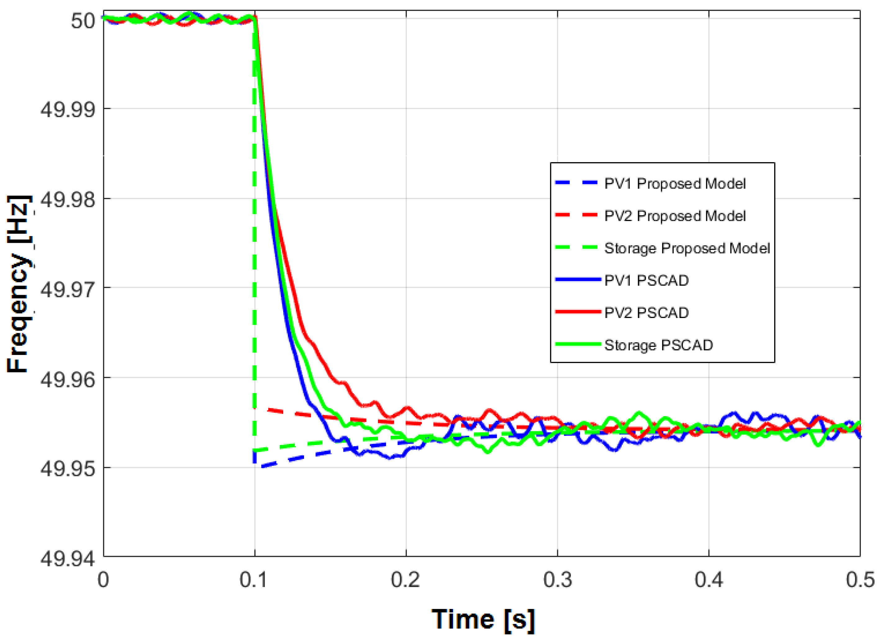
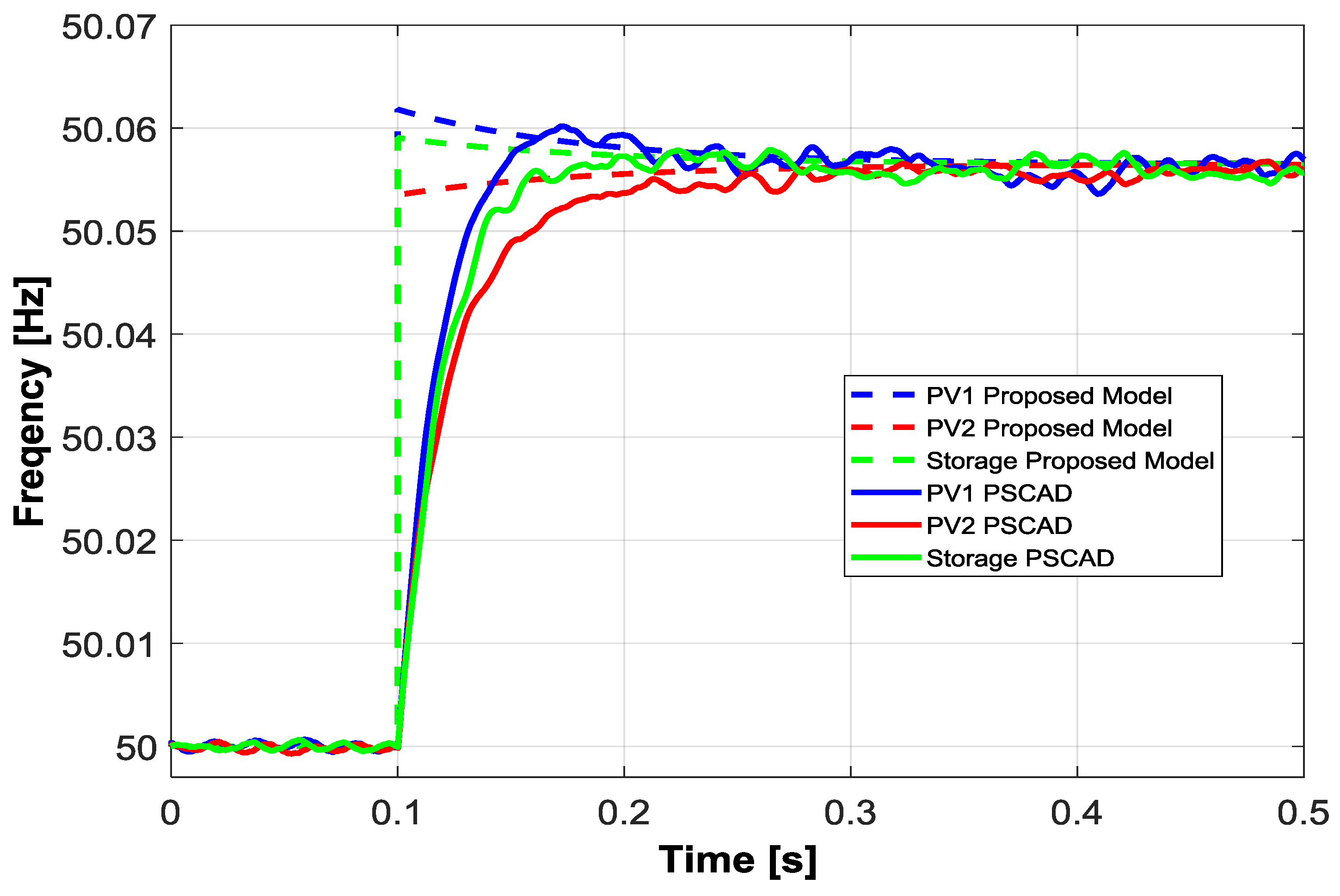
In particular, the dynamics predicted by the proposed approach are much faster than the PSCAD ones; this is due to the fact that one of the main assumptions supporting the developed model supposes the AC portion of the network to be at steady state. Moreover, as demonstrated in [28], the sources’ frequencies reach the same steady state value (see Figure 12). This allows the quantification of the active power sharing and the steady-state frequency deviation, equal to −0.045 Hz. From the comparison point of view, the same considerations can be made as in the previous figures concerning the ability of the simplified model to effectively predict the steady-state value with a much faster dynamic.
As far as the state variables are concerned, Figure 13 and Figure 14 highlight that, both in the transient and in the steady-state, the developed approach shows an excellent agreement with the PSCAD simulations.
Moreover, it can be noted that the increase of the load active power claims for the injection of a higher amount of current by the storage; firstly, this current is supplied by the DC link storage capacitor, which causes a voltage dip of about 0.04 s. Finally, due to the fact that the initial PVs’ voltages are over the VMPP (653.4 V and 712.8 V respectively), when the droop control requires the PVs to inject a higher amount of power, the DC voltages decrease.
Finally, Figure 15 plots the Q2 voltage amplitude according to the simplified model and to the PSCAD simulation; again, it is possible observing the quite good agreement characterized by an error smaller than 0.5%.
6.1.2. Active Power Decreasing Simulation (S2)
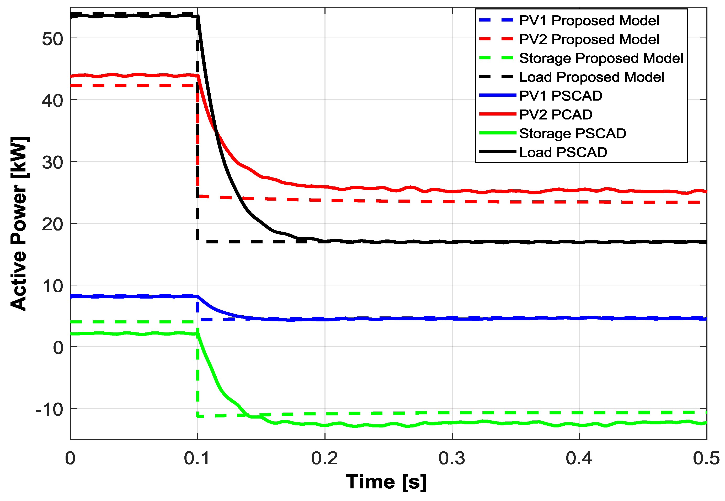
The initial point of the active power decreasing simulation is the same as that used for the active power increasing test case (see Table 8). The contingency occurs at 0.1 s and consists of a step change in the load resistance from 3 Ω to 10 Ω (corresponding to 53 and 16 kW respectively), Figure 16 shows the active power behavior, highlighting a good agreement between the two approaches, with some small deviations in the steady-state values of the power provided by the storage and the bigger PV unit. As far as the transient behavior is concerned, the same considerations as before can be made. The active power sharing among the sources and the final value of the system frequency can be appreciated examining Figure 17 in which a frequency deviation of +0.056 Hz occurs.
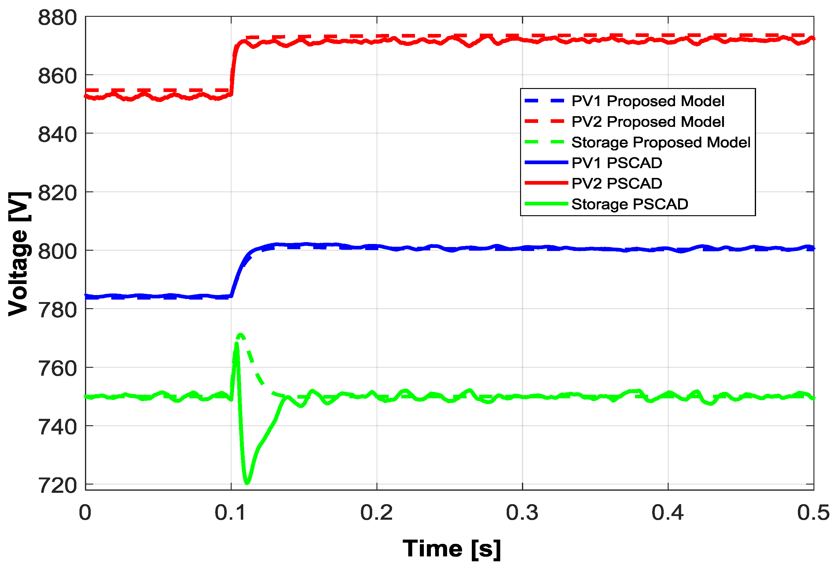
Due to the fact that the initial PVs’ voltages are over VMPP, (653.4 V and 712.8 V respectively), the decrease of the active power production determines an increase in the DC voltages (Figure 18).
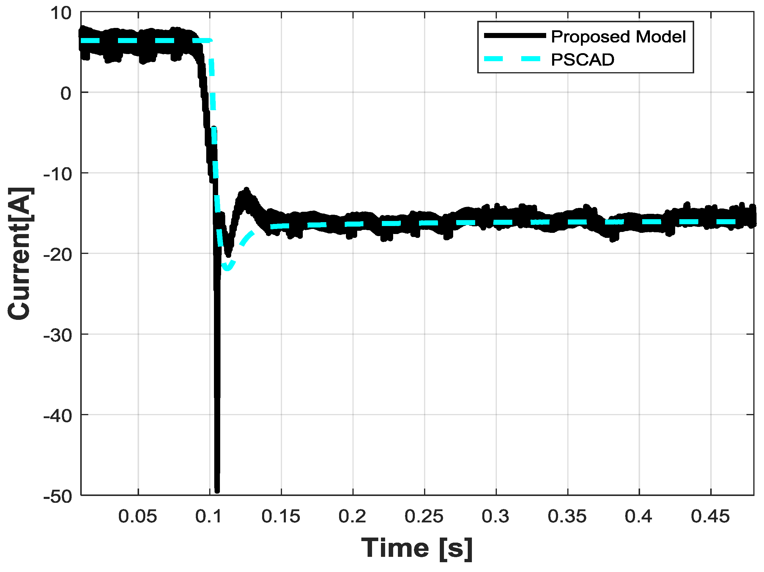
The effect of the contingency on the storage system is that it starts absorbing power, which is allowed by a change in the sign of the current. Firstly, this current is absorbed by the DC link storage capacitor; in fact, in Figure 18, an overvoltage transient of about 0.03 s occurs in the proposed model, while an overvoltage transient of about 0.01 s occurs in the complete one. The current behavior is proposed in Figure 19. This different dynamic is due to a discontinuous conduction mode, typical of DC/DC converters when dealing with low current values [46]. This phenomenon is extinguished when the active power inverts its sign activating the buck converter control.
Finally, the examination of the voltage at Q2 bus highlights again the good performances of the simplified model and the fact that, after this perturbation, such a voltage still lies inside the feasible range (±5% of its rated value) (Figure 20).
6.2. Isochronous Control Simulations
Two simulations performed to verify the performances of the proposed model with the isochronous controller are presented here.
6.2.1. Active Power Increasing Simulation (S3)
The first simulation starts from the initial states appearing in Table 9 and consists of a reduction of the load resistance from 3 to 1.2 Ω (corrisponding to 53 and 130 kW) at 0.1 seconds from the beginning of the simulation (again carried out at constant conditions of external temperature and solar radiation).
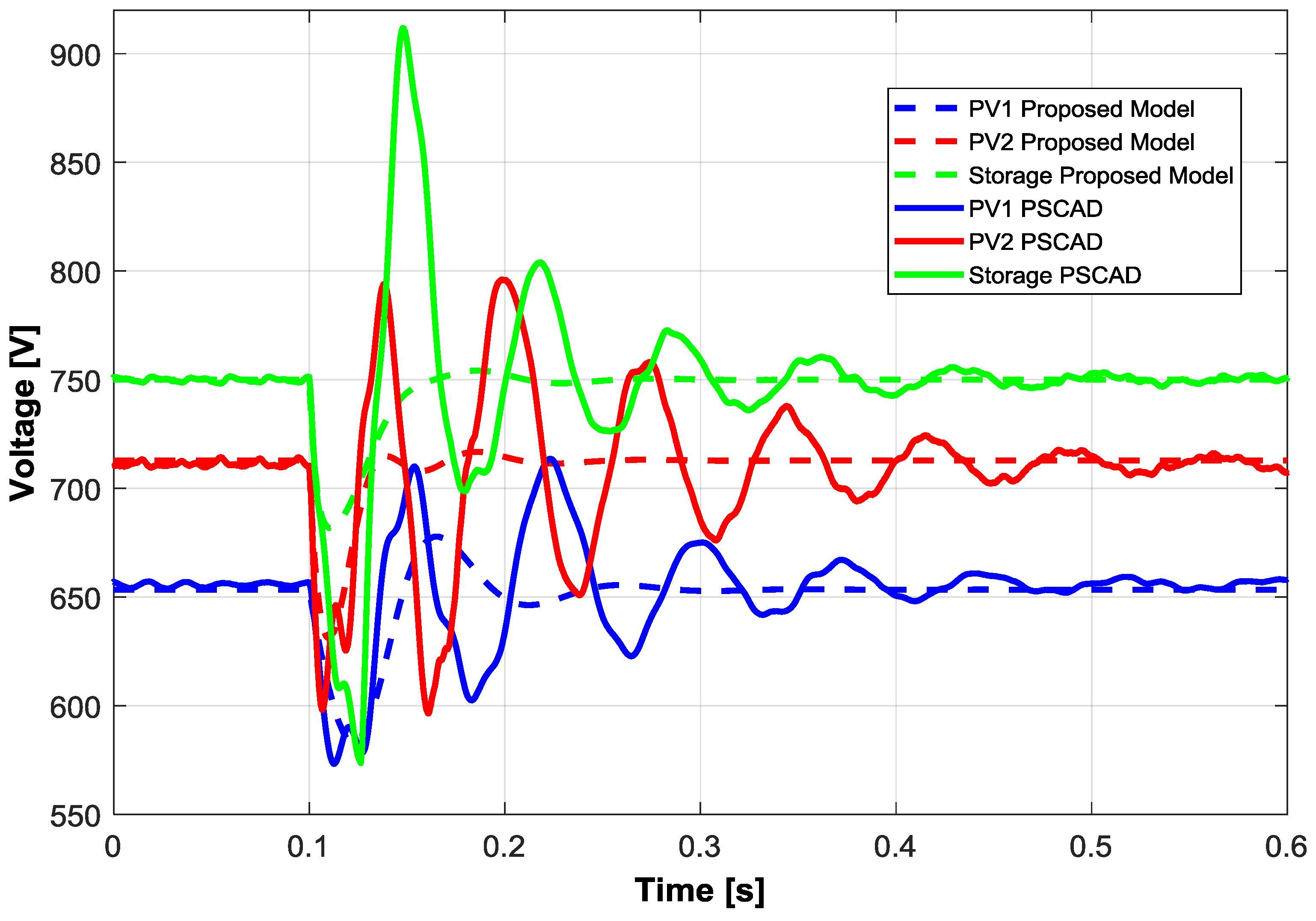
The increase of active power is fully provided by the storage, as shown in Figure 21. This implies that the storage current increases to a positive value; firstly, this current is supplied by the DC link storage capacitor causing a voltage dip (Figure 22). The different storage DC voltage dynamic behaviour of the two models shown in Figure 22 is due to a discontinuous conduction mode, typical of DC/DC converters when dealing with low current values [46]. This phenomenon, that can also be noticed in Figure 23, is extinguished when the active power changes its sign and activates the boost converter control. On the other hand, the final working point of the PV units is the same as the pre-contingency one, according to their power control mode.
Performing a comparison, it can be observed that the simplified model is not able to capture the oscillatory transients caused by the perturbation; however, a very good agreement is obtained in the steady-state behavior reproduction.
The prediction of the behavior of the voltage at Q2 bus is quite satisfactory (see Figure 24) as the simplified model is able to capture both the initial voltage dip (with a slight underestimation of its amplitude) and the final working point (laying inside the range of ±5% of the rated value).
6.2.2. Double Perturbation Simulation (S4)
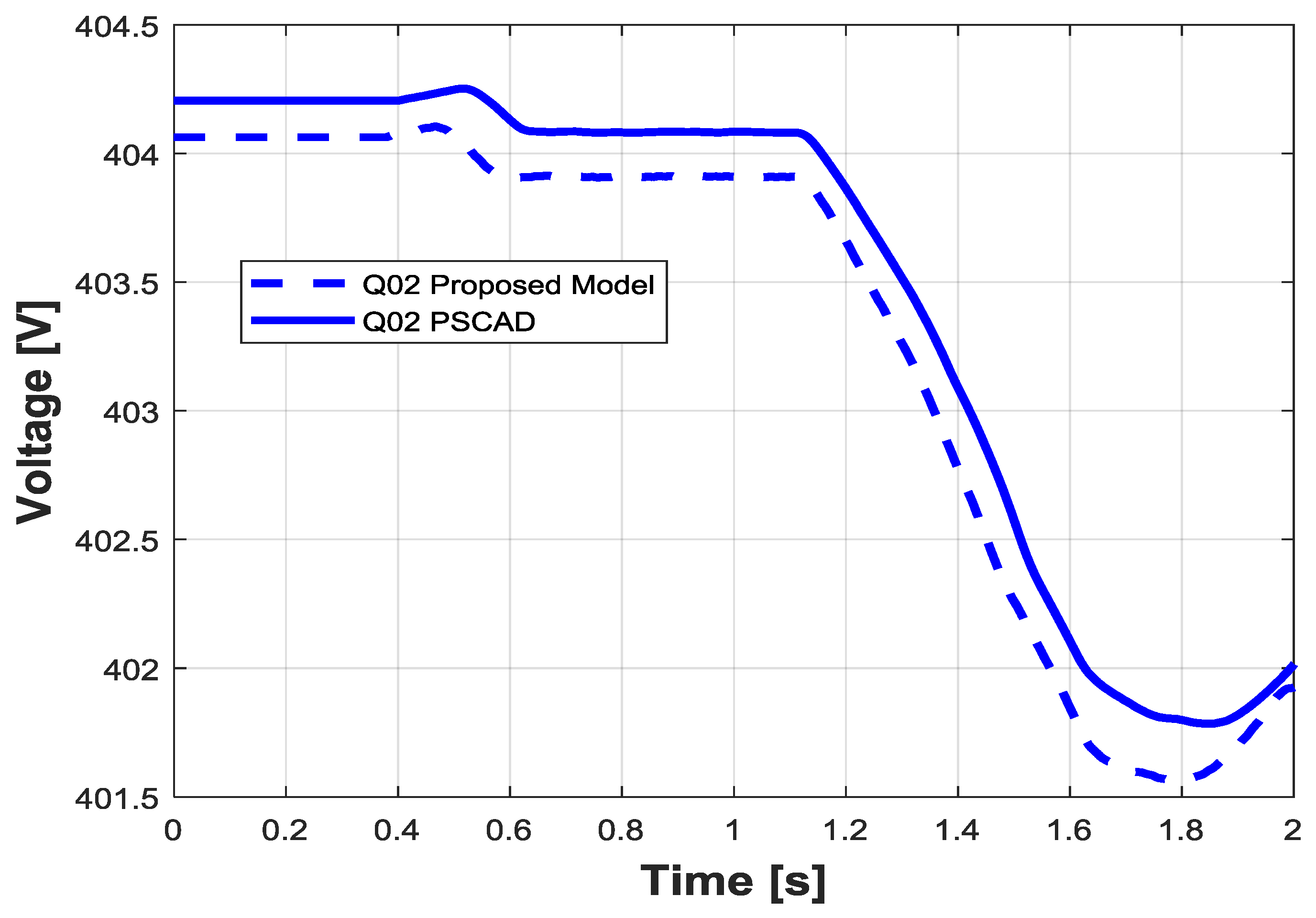
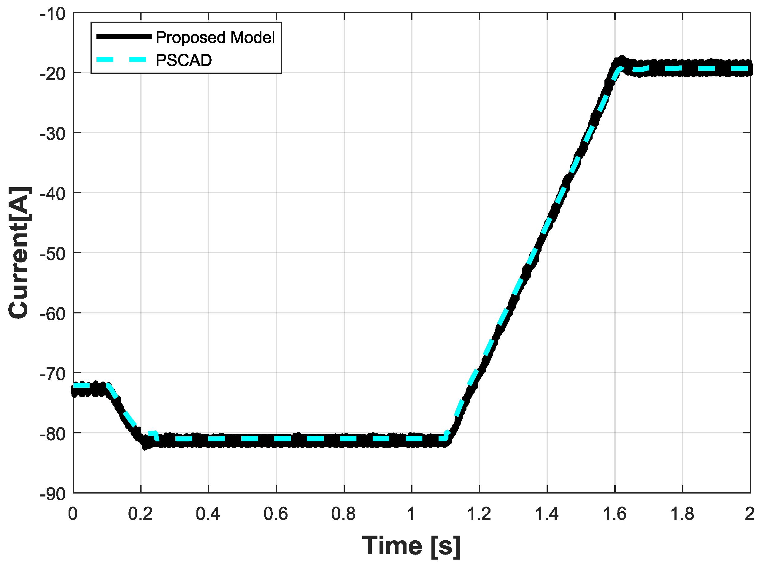
The second simulation concerning the isochronous control logic consists of a double variation in the same scenario. In particular, a load variation and an irradiance decreasing according to two different ramp profiles are presented here. The load variation starts at 0.1 s and consists of an decreasing of the active power absorbed by the load from 39 to 31 kW in 0.1 s, while the decreasing irradiance consists of a halving from 1000 to 500 W/m2 in 0.5 s starting at 1.1 s. The initial states of the simulation are provided in Table 10.
When the ramp variation load occurs, the storage must absorb more active power (Figure 25) in order to guarantee the active power balance. The DC PV and storage voltages and the DC storage current are not affected by this variation, except for a brief transient. This can be ascribed to the fact that a ramp variation causes fewer problems in the dynamic response than a step variation as in the previous simulations. When the irradiance decreases each PV unit supplies less active power (Figure 25) and according to their control mode the DC voltages decrease to the new VMPP (Figure 26).
As can be seen in Figure 27, the Q2 bus voltage is always between the acceptable limits and has some small variations according to the variation described above. Analogue conclusions can be drawn for LST current, shown in Figure 28.
In all the figures presented, the agreement in the dynamic response between the proposed and the PSCAD models is improved with respect to the previous simulations S3. Indeed, the ramp variations affect the dynamic response less than a step variation; thus, what can be concluded is that the smoother is the dynamic variation, the better the agreement between the two models.
7. Conclusions
This paper presented a simplified modelling approach to study the behavior of MGs characterized by all of the generation being interfaced to the AC part of the MG by means of power electronic devices in an islanded configuration. The aim of the article was to define a simplified but effective representation for this kind of MGs, in order to provide a useful and reliable tool for the validation of innovative control strategies for islanded MGs. The proposed model can be described by a system of ordinary differential equations that can be implemented in a general-purpose software with a reduced computational effort. The peculiarity of the proposed methodology is that it is not suited for a specific control strategy or MG structure, but can be adapted and implemented for different control strategies, topologies and generation mixes. Contrary to other simplified MG models, the proposed model accounts for power losses, voltage drops, DC voltage and frequency dynamics; these are the reasons why it is fit to be used as an environment to implement and test primary frequency and voltage control logics. Moreover, the usefulness of the proposed model is represented by the simulation time-saving with respect to traditional power system simulators and by the possibility to handle the MG dynamics without licensed and specific software. The effectiveness and the good trade-offs of the proposed model have been evaluated by means of a comparison with a detailed representation of a MG test case in the PSCAD-EMTDC environment. In order to account for a realistic test case characterized by known parameters and control logics, the proposed methodology was tested modeling the islanded portion of the SPM of the Savona Campus of Genoa University. This MG can be operated with two different island control strategies; the droop and isochronous strategies. Simulations performed with both the previously mentioned control strategies highlighted the good behavior of the proposed model, particularly if one considers the elements that are relevant with respect to the characterization of the system for a primary frequency and voltage control validation purpose.
Future work will imply the validation of the proposed model against experimental measurements that can be performed in the SPM and the use of the simplified model to develop and assess the performances of more advanced controllers—e.g., an MPC based controller—before their actual implementation in the SPM.
Author Contributions
Marco Invernizzi and Renato Procopio outline the basic theories behind the research work; Massimo Brignone and Andrea Bonfiglio elaborate the system control equations; Alessandro Labella and Daniele Mestriner conceived and designed the experiments, performed the experiments and analyzed the data. All the authors wrote the paper.
Conflicts of Interest
The authors declare no conflict of interest.
Nomenclature
| Acronyms | |
| SQ | Switchgear |
| PV | Photovoltaic source |
| SPM | Smart Polygeneration Microgrid |
| Variables | |
| α | Solar irradiation |
| T | External temperature |
| SOC | State of charge |
| δk | Angle of the k-th source |
| φk | Phase of the k-th source |
| ωk | Angular frequency of the k-th source |
| mk | Modulation index of the k-th source |
| Voltage phasor of the k-th source | |
| Current phasor of the k-th source | |
| VDC,k | Voltage across the capacitor |
| IST | LST current |
| E | Storage internal e.m.f. |
| VMPP | Maximum power point voltage at specified conditions |
| χ1 | Integrator control output of boost level of DC/DC converter |
| χ2 | Integrator control output of buck level of DC/DC converter |
| η1,k | Integrator control output of active power control of the k-th source |
| η2,k | Integrator control output of reactive power control of the k-th source |
| YE | Extended admittance matrix |
| Gi,k | Real part of the i-k-th element of YE |
| Bi,k | Imaginary part of the i-k-th element of YE |
| VDC,k | Voltage across the Ck |
| Constants | |
| Rint | Internal resistance of the chemical storage |
| LST | Storage side inductance filter of DC/DC converter |
| Ck | DC capacitor of the k-th inverter |
| mD,k | Active power droop coefficient of the k-th source |
| nD,k | Reactive power droop coefficient of the k-th source |
| NCC | Storage nominal current capacity |
| Indices | |
| k | Index of sources; 1 refers to PV1, 2 to PV2, 3 to storage |
| i | Auxiliary index for k |
| Functions | |
| f | Function describing ODE system without control |
| fD | Function describing ODE system with droop logic |
| fI | Function describing ODE system with isochronous logic |
| gD | Function describing algebraic equations subsystem with droop logic |
| gI | Function describing algebraic equations subsystem with isochronous logic |
| KST | Voltage DC/DC converter transfer function |
References
- Hatziargyriou, N.; Asano, H.; Iravani, R.; Marnay, C. Microgrids. Microgrids. IEEE Power Energy Mag. 2007, 5, 78–94. [Google Scholar] [CrossRef]
- Sun, I.; Kim, S. Energy R&D towards Sustainability: A Panel Analysis of Government Budget for Energy R&D in OECD Countries (1974–2012). Sustainability 2017, 9, 617. [Google Scholar]
- Ardito, L.; Procaccianti, G.; Menga, G.; Morisio, M. Smart Grid Technologies in Europe: An Overview. Energies 2013, 6, 251. [Google Scholar] [CrossRef]
- Gonzalez-Longatt, F.M.; Bonfiglio, A.; Procopio, R.; Verduci, B. Evaluation of inertial response controllers for full-rated power converter wind turbine (Type 4). In Proceedings of the IEEE Power and Energy Society General Meeting, Boston, MA, USA, 17–21 July 2016; pp. 1–5. [Google Scholar]
- Pichetjamroen, A.; Ise, T. Power Control of Low Frequency AC Transmission Systems Using Cycloconverters with Virtual Synchronous Generator Control. Energies 2017, 10, 34. [Google Scholar] [CrossRef]
- Bonfiglio, A.; Brignone, M.; Delfino, F.; Invernizzi, M.; Pampararo, F.; Procopio, R. A technique for the optimal control and operation of grid-connected photovoltaic production units. In Proceedings of the 2012 47th International Universities Power Engineering Conference, London, UK, 4–7 September 2012; pp. 1–6. [Google Scholar]
- Delfino, B.; Fornari, F.; Procopio, R. An effective SSC control scheme for voltage sag compensation. IEEE Trans. Power Deliv. 2005, 20, 2100–2107. [Google Scholar] [CrossRef]
- Fornari, F.; Procopio, R.; Bollen, M.H.J. SSC compensation capability of unbalanced voltage sags. IEEE Trans. Power Deliv. 2005, 20, 2030–2037. [Google Scholar] [CrossRef]
- Manitoba-HVDC. PSCAD Library. Available online: https://hvdc.ca/knowledge-library/reference-material (accessed on 23 July 2017).
- PartSim. SPICE Simulator. Available online: www.partsim.com/simulator (accessed on 23 July 2017).
- Plexim. PLECS. Available online: https://www.plexim.com/ (accessed on 23 July 2017).
- Bendato, I.; Bonfiglio, A.; Brignone, M.; Delfino, F.; Pampararo, F.; Procopio, R. Definition and On-Field Validation of a Microgrid Energy Management System to manage Load and Renewables Uncertainties and System Operator Requirements. Electric Power Syst. Res. J. 2017, 146, 349–361. [Google Scholar] [CrossRef]
- Porsinger, T.; Janik, P.; Leonowicz, Z.; Gono, R. Modelling and Optimization in Microgrids. Energies 2017, 10, 523. [Google Scholar] [CrossRef]
- Aman, S.; Simmhan, Y.; Prasanna, V.K. Energy management systems: State of the art and emerging trends. IEEE Community Mag. 2013, 51, 114–119. [Google Scholar] [CrossRef]
- Lopes, J.A.P.; Moreira, C.L.; Madureira, A.G. Defining control Strategies for Microgrids islanded Operations. IEEE Trans. Power Syst. 2006, 21, 916–924. [Google Scholar] [CrossRef]
- Dall’Anese, E.; Zhu, H.; Giannakis, G.B. Distributed optimal power flow for smart microgrids. IEEE Trans. Smart Grid 2013, 4, 1464–1475. [Google Scholar] [CrossRef]
- Bonfiglio, A.; Delfino, F.; Invernizzi, M.; Labella, A.; Mestriner, D.; Procopio, R.; Serra, P. Approximate characterization of large Photovoltaic power plants at the Point of Interconnection. In Proceedings of the 2015 50th International Universities Power Engineering Conference (UPEC), Stoke-on-Trent, UK, 1–4 September 2015. [Google Scholar]
- Muljadi, E.; Butterfield, C.P.; Ellis, A.; Mechenbier, J.; Hochheimer, J.; Young, R.; Miller, N.; Delmerico, R.; Zavadil, R.; Smith, J.C. Equivalencing the collector system of a large wind power plant. In Proceedings of the IEEE Power Engineering Society General Meeting, Montreal, QC, Canada, 18–22 June 2006. [Google Scholar]
- Bonfiglio, A.; Delfino, F.; Invernizzi, M.; Serra, P.; Procopio, R. Criteria for the Equivalent Modeling of Large Photovoltaic Power Plants. In Proceedings of the IEEE Power and Energy Society General Meeting, National Harbor, MD, USA, 27–31 July 2014. [Google Scholar]
- Changchun, C.; Lihua, D.; Weili, D.; Jianyong, Z. Characteristic model based micro-grid equivalent modeling. In Proceedings of the 2014 International Conference on Power System Technology, Chengdu, China, 20–22 October 2014; pp. 3035–3040. [Google Scholar]
- Hussain, A.; Bui, V.H.; Kim, H.M. Robust Optimization-Based Scheduling of Multi-Microgrids Considering Uncertainties. Energies 2016, 9, 278. [Google Scholar] [CrossRef]
- Ahn, C.; Peng, H. Decentralized and Real-Time Power Dispatch Control for an Islanded Microgrid Supported by Distributed Power Sources. Energies 2013, 6, 6439. [Google Scholar] [CrossRef]
- Hernandez, L.; Baladrón, C.; Aguiar, J.; Carro, B.; Sanchez-Esguevillas, A.; Lloret, J. Short-Term Load Forecasting for Microgrids Based on Artificial Neural Networks. Energies 2013, 6, 1385. [Google Scholar] [CrossRef]
- Basak, P.; Saha, A.K.; Chowdhury, S.; Chowdhury, S.P. Microgrid: Control techniques and modeling. In Proceedings of the 2009 44th International Universities Power Engineering Conference (UPEC), Glasgow, UK, 1–4 September 2009; pp. 1–5. [Google Scholar]
- Bonfiglio, A.; Barillari, L.; Brignone, M.; Delfino, F.; Pampararo, F.; Procopio, R.; Rossi, M.; Bracco, S.; Robba, M. An optimization algorithm for the operation planning of the University of Genoa smart polygeneration microgrid. In Proceedings of the 2013 IREP Symposium Bulk Power System Dynamics and Control—IX Optimization, Security and Control of the Emerging Power Grid, Rethymno, Greece, 25–30 August 2013. [Google Scholar]
- Hou, X.; Sun, Y.; Yuan, W.; Han, H.; Zhong, C.; Guerrero, J. Conventional P-ω/Q-V Droop Control in Highly Resistive Line of Low-Voltage Converter-Based AC Microgrid. Energies 2016, 9, 943. [Google Scholar] [CrossRef]
- MChandorkar, C.; Divan, D.M.; Adapa, R. Control of parallel connected inverters in standalone AC supply systems. IEEE Trans. Ind. Appl. 1993, 29, 136–143. [Google Scholar] [CrossRef]
- Labella, A.; Mestriner, D.; Procopio, R.; Brignone, M. A new method to evaluate the stability of a droop controlled micro grid. In Proceedings of the 2017 10th International Symposium on Advanced Topics in Electrical Engineering (ATEE), Bucharest, Romania, 23–25 March 2017; pp. 448–453. [Google Scholar]
- Bidram, A.; Davoudi, A. Hierarchical Structure of Microgrids Control System. IEEE Trans. Smart Grid 2012, 3, 1963–1976. [Google Scholar] [CrossRef]
- Guerrero, J.M.; Loh, P.C.; Lee, T.L.; Chandorkar, M. Advanced Control Architectures for Intelligent Microgrids—Part II. IEEE Trans. Ind. Electron. 2013, 60, 1263–1270. [Google Scholar] [CrossRef]
- Guerrero, J.M.; Chandorkar, M.; Lee, T.L.; Loh, P.C. Advanced control architectures for intelligent microgrids—Part I: Decentralized and hierarchical control. IEEE Trans. Ind. Electron. 2013, 60, 1254–1262. [Google Scholar] [CrossRef]
- Su, X.; Han, M.; Guerrero, J.; Sun, H. Microgrid Stability Controller Based on Adaptive Robust Total SMC. Energies 2015, 8, 1784. [Google Scholar] [CrossRef]
- Chlela, M.; Mascarella, D.; Joos, G.; Kassouf, M. Fallback Control for Isochronous Energy Storage Systems in Autonomous Microgrids Under Denial-of-Service Cyber-Attacks. IEEE Trans. Smart Grid 2017, PP, 1. [Google Scholar] [CrossRef]
- Xiao, S.; Yim-Shu, L.; Dehong, X. Modeling, analysis, and implementation of parallel multi-inverter systems with instantaneous average-current-sharing scheme. IEEE Trans. Power Electron. 2003, 18, 844–856. [Google Scholar] [CrossRef]
- Parisio, A.; Rikos, E.; Glielmo, L. A Model Predictive Control Approach to Microgrid Operation Optimization. IEEE Trans. Control Syst. Technol. 2014, 22, 1813–1827. [Google Scholar] [CrossRef]
- Nguyen, T.T.; Yoo, H.J.; Kim, H.M. Analyzing the Impacts of System Parameters on MPC-Based Frequency Control for a Stand-Alone Microgrid. Energies 2017, 10, 417. [Google Scholar] [CrossRef]
- Kerdphol, T.; Rahman, F.; Mitani, Y.; Hongesombut, K.; Küfeoğlu, S. Virtual Inertia Control-Based Model Predictive Control for Microgrid Frequency Stabilization Considering High Renewable Energy Integration. Sustainability 2017, 9, 773. [Google Scholar] [CrossRef]
- Bonfiglio, A.; Delfino, F.; Invernizzi, M.; Perfumo, A.; Procopio, R. A feedback linearization scheme for the control of synchronous generators. Electric Power Compon. Syst. 2012, 40, 1842–1869. [Google Scholar] [CrossRef]
- Bonfiglio, A.; Delfino, F.; Pampararo, F.; Procopio, R.; Rossi, M.; Barillari, L. The Smart Polygeneration Microgrid test-bed facility of Genoa University. In Proceedings of the 47th International Universities Power Engineering Conference, London, UK, 4–7 September 2012. [Google Scholar]
- Bell, K.R.W.; Tleis, A.N.D. Test system requirements for modelling future power systems. In Proceedings of the 2010 IEEE Power and Energy Society General Meeting, Providence, RI, USA, 25–29 July 2010; pp. 1–8. [Google Scholar]
- Böke, U. A simple model of photovoltaic module electric characteristics. In Proceedings of the European Conference on Power Electronics and Applications, Aalborg, Denmark, 2–5 September 2007. [Google Scholar]
- FIAMM. SoNick ST523. Available online: Fiamm.com/media/20150209-st523_datasheet.pdf (accessed on 21 July 2017).
- Rexed, I.; Behm, M.; Lindbergh, G. Modelling of ZEBRA Batteries; Royal Institute of Technology. Available online: https://www.kth.se/polopoly_fs/1.187945!/Menu/general/column-content/attachment/59.pdf (accessed on 21 July 2017).
- Sudworth, J.L. Zebra batteries. J. Power Sources 1994, 51, 105–114. [Google Scholar] [CrossRef]
- Seyedmahmoudian, M.; Mekhilef, S.; Rahmani, R.; Yusof, R.; Renani, E. Analytical Modeling of Partially Shaded Photovoltaic Systems. Energies 2013, 6, 128. [Google Scholar] [CrossRef] [Green Version]
- Erickson, R.; Maksimovic, D. Fundamentals of Power Electronics, 2nd ed.; Springer US: London, UK, 2004; pp. 1–883. [Google Scholar]
- Kundur, P.; Balu, N.J.; Lauby, M.G. Power System Stability and Control; McGraw-Hill: Palo Alto, CA, USA, 1994; pp. 1–1200. [Google Scholar]
- Guerrero, J.M.; Vasquez, J.C.; Matas, J.; Vicuna, L.G.; Castilla, M. Hierarchical Control of Droop-Controlled AC and DC Microgrids—A General Approach toward Standardization. IEEE Trans. Ind. Electron. 2011, 58, 158–172. [Google Scholar] [CrossRef]
- Simpson-Porco, J.W.; Dörfler, F.; Bullo, F. Synchronization and power sharing for droop-controlled inverters in islanded microgrids. Automatica 2013, 49, 2603–2611. [Google Scholar] [CrossRef]
- Mohd, A.; Ortjohann, E.; Sinsukthavorn, W.; Lingemann, M.; Hamsic, N.; Morton, D. Isochronous load sharing and control for inverter-based distributed generation. In Proceedings of the 2009 International Conference on Clean Electrical Power, Capri, Italy, 9–11 June 2009; pp. 324–329. [Google Scholar]
- Kim, J.Y.; Jeon, J.H.; Kim, S.K.; Cho, C.; Park, J.H.; Kim, H.M.; Nam, K. Cooperative Control Strategy of Energy Storage System and Microsources for Stabilizing the Microgrid during Islanded Operation. IEEE Trans. Power Electron. 2010, 25, 3037–3048. [Google Scholar]
- Milano, F. Power system modelling and scripting. In Power Systems; Springer: London, UK, 2010; Volume 54, pp. 1–550. [Google Scholar]
- Delfino, F.; Procopio, R.; Rossi, M.; Ronda, G. Integration of large-size photovoltaic systems into the distribution grids: A P-Q chart approach to assess reactive support capability. IET Renew. Power Gener. 2010, 4, 329–340. [Google Scholar] [CrossRef]
Figure 1.
Graphical representation of the proposed concept of defining a simplified model that can be used with various control strategies.
Figure 1.
Graphical representation of the proposed concept of defining a simplified model that can be used with various control strategies.

Figure 2.
Smart Polygeneration Microgrid (SPM) portion used to create the island.
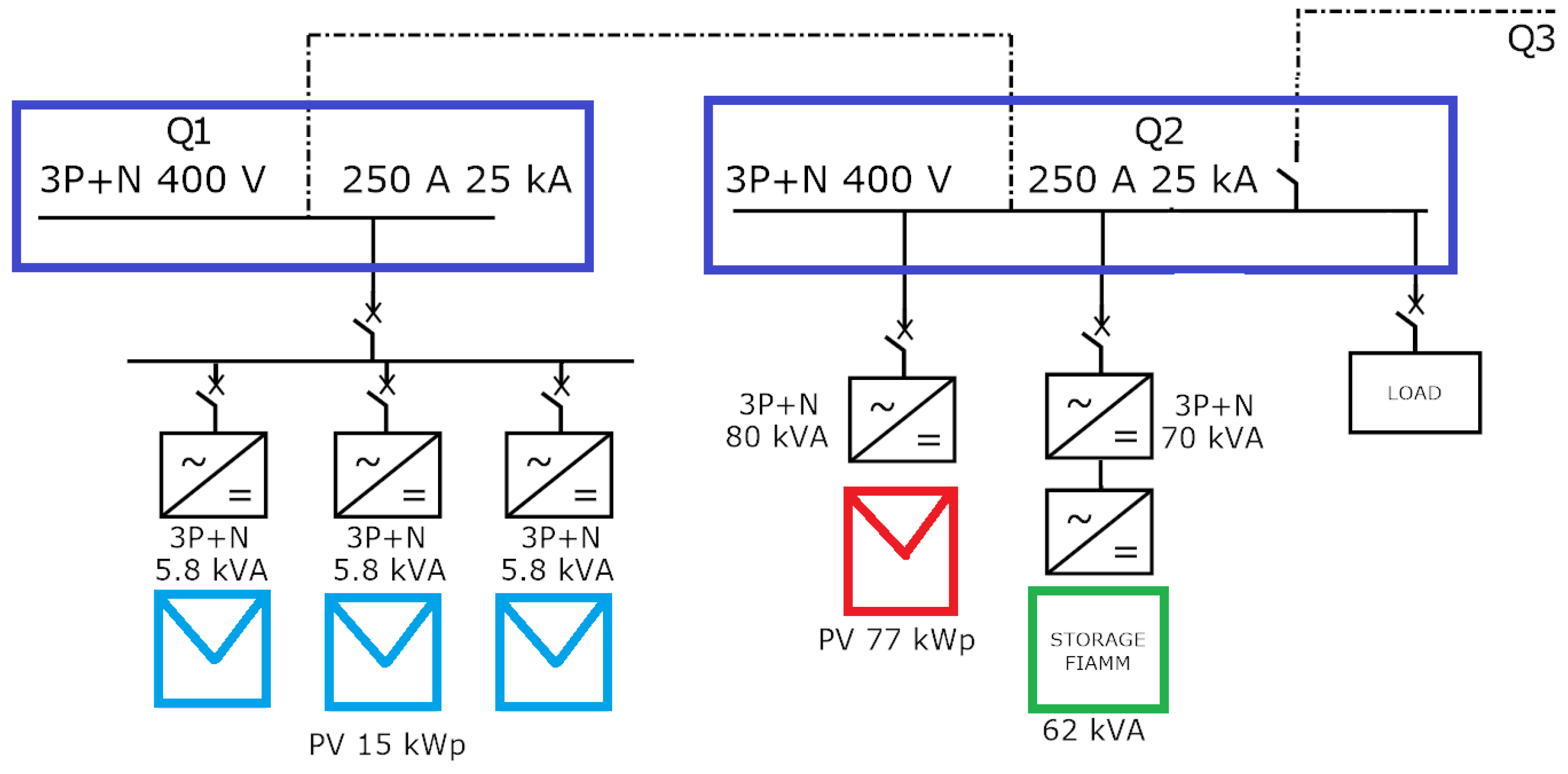

Figure 4.
Voltage against SOC cell characteristic

Figure 5.
Inverter AC filter configuration.

Figure 6.
DC/DC converter circuital layout.

Figure 7.
Simplified model of the islanded portion of the SPM.
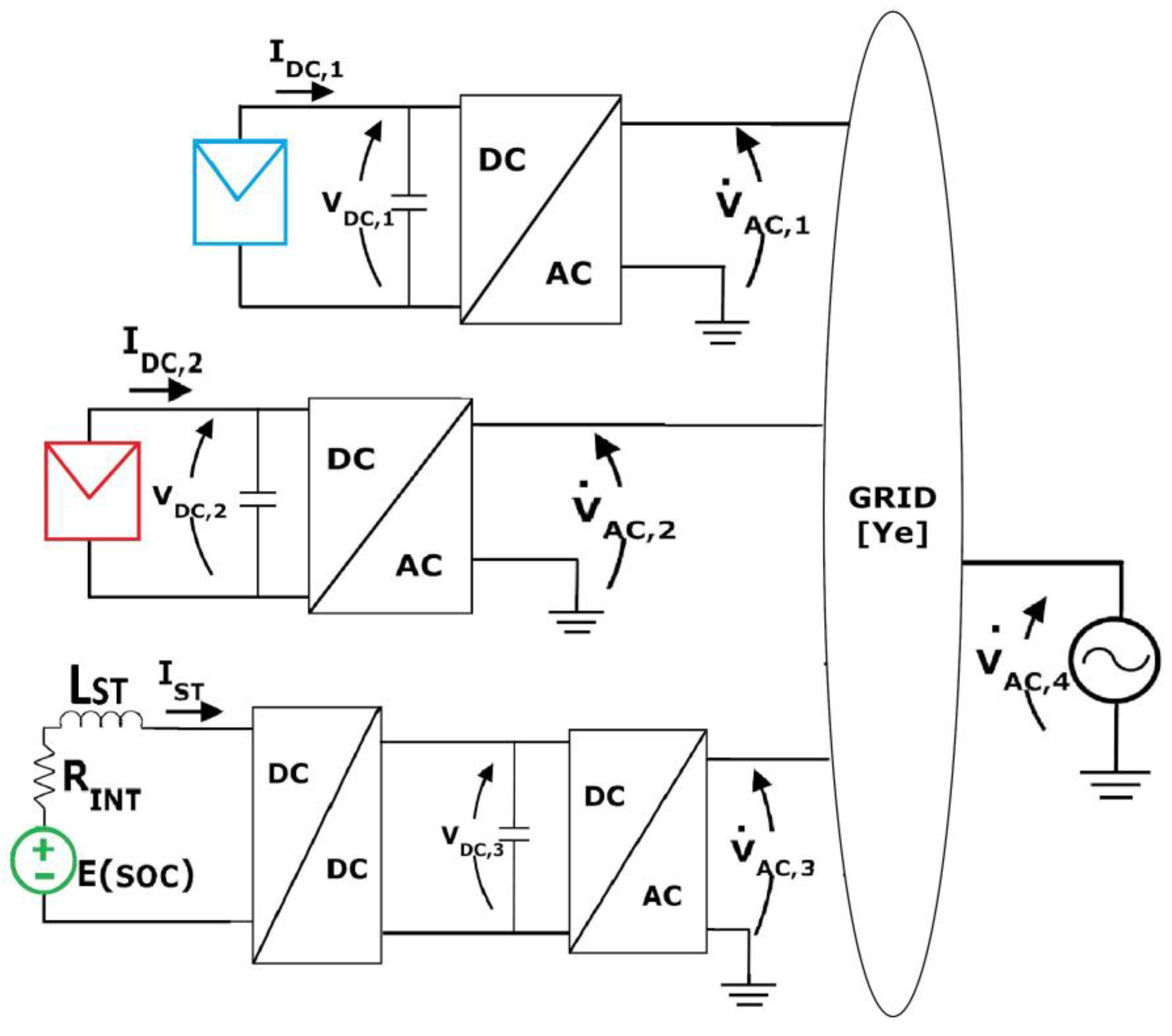
Figure 8.
Block scheme droop strategy.
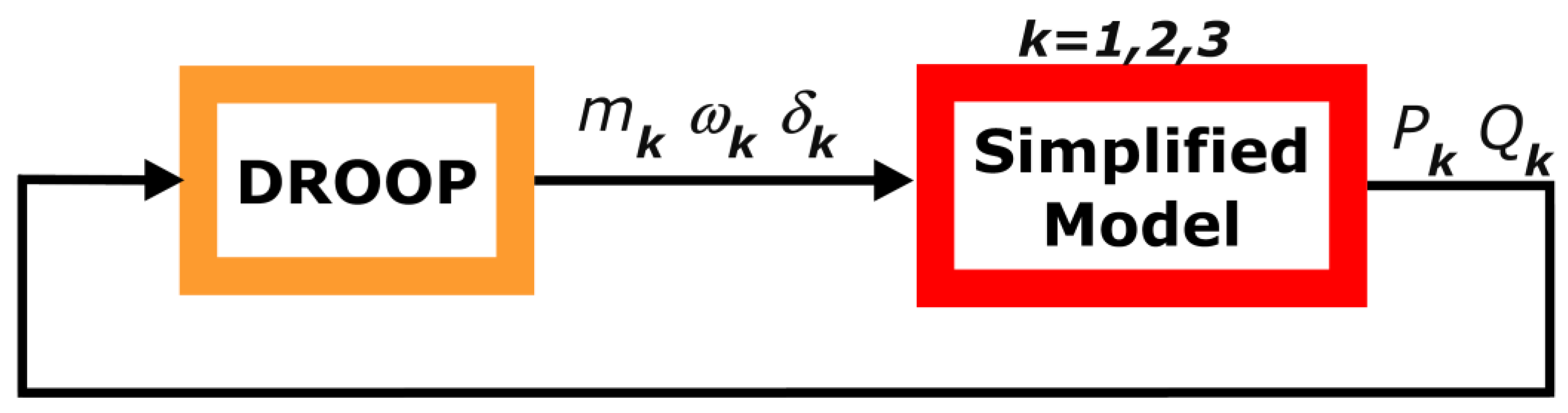
Figure 9.
Block scheme isochronous strategy.

Figure 10.
PSCAD model overview
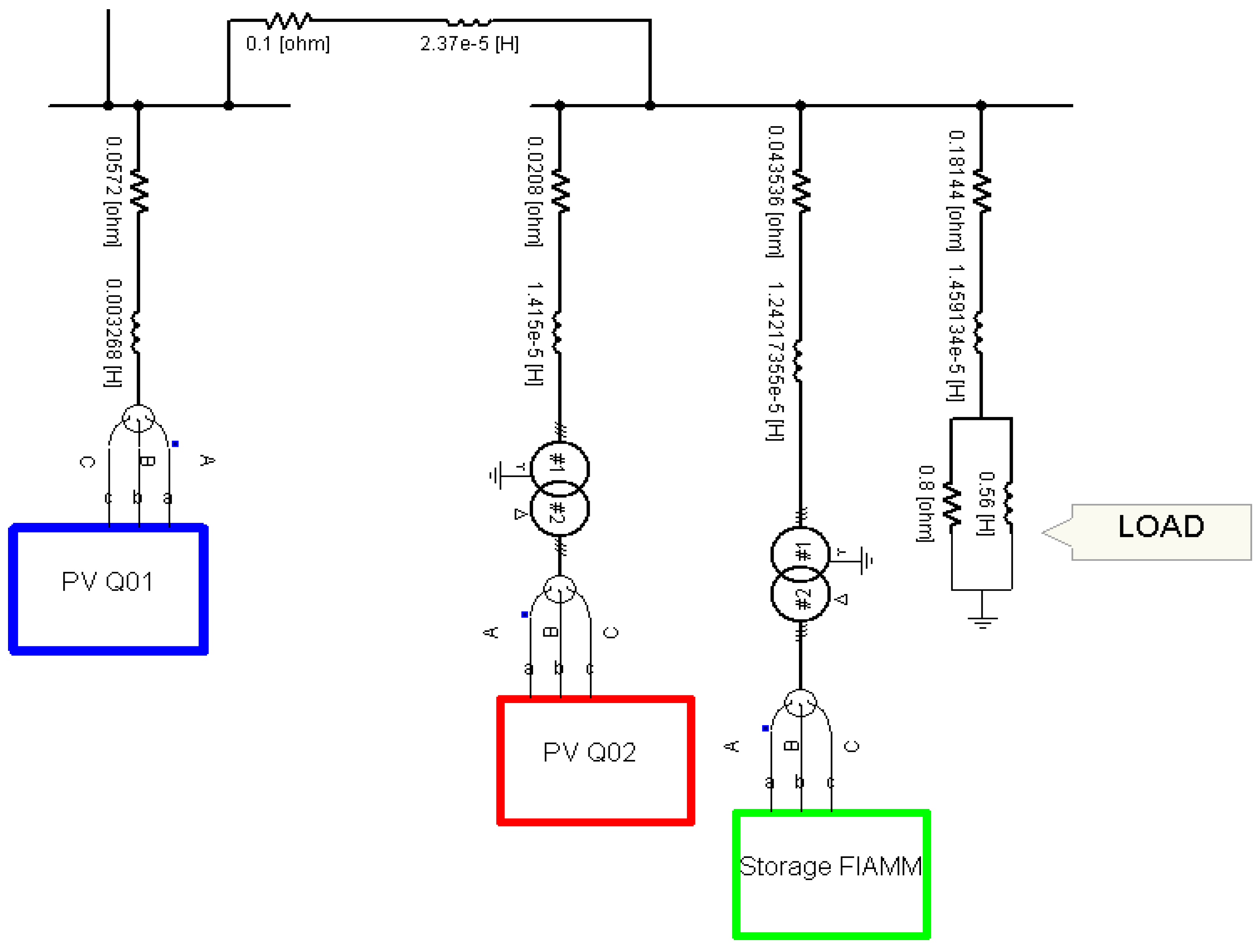
Figure 11.
Active power time profile for load increasing scenario; the solid lines refers to PSCAD model while dashed ones refer to the proposed approach.
Figure 11.
Active power time profile for load increasing scenario; the solid lines refers to PSCAD model while dashed ones refer to the proposed approach.

Figure 12.
Frequencies output time profile for the load increasing scenario; the solid lines refer to PSCAD model while dashed ones refer to the proposed approach.
Figure 12.
Frequencies output time profile for the load increasing scenario; the solid lines refer to PSCAD model while dashed ones refer to the proposed approach.

Figure 13.
DC capacitor voltage time profile for the load increasing scenario; the solid lines refer to PSCAD model while dashed ones refer to the proposed approach.
Figure 13.
DC capacitor voltage time profile for the load increasing scenario; the solid lines refer to PSCAD model while dashed ones refer to the proposed approach.
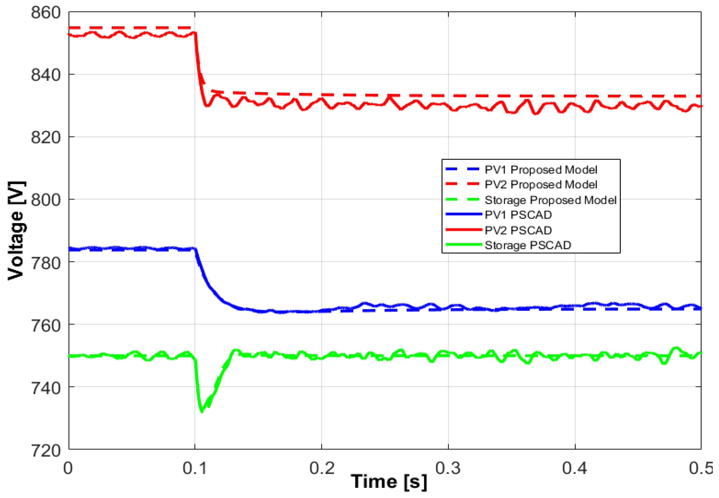
Figure 14.
LST current profile for the load increasing scenario; the solid lines refer to PSCAD model while dashed ones refer to the proposed approach.
Figure 14.
LST current profile for the load increasing scenario; the solid lines refer to PSCAD model while dashed ones refer to the proposed approach.
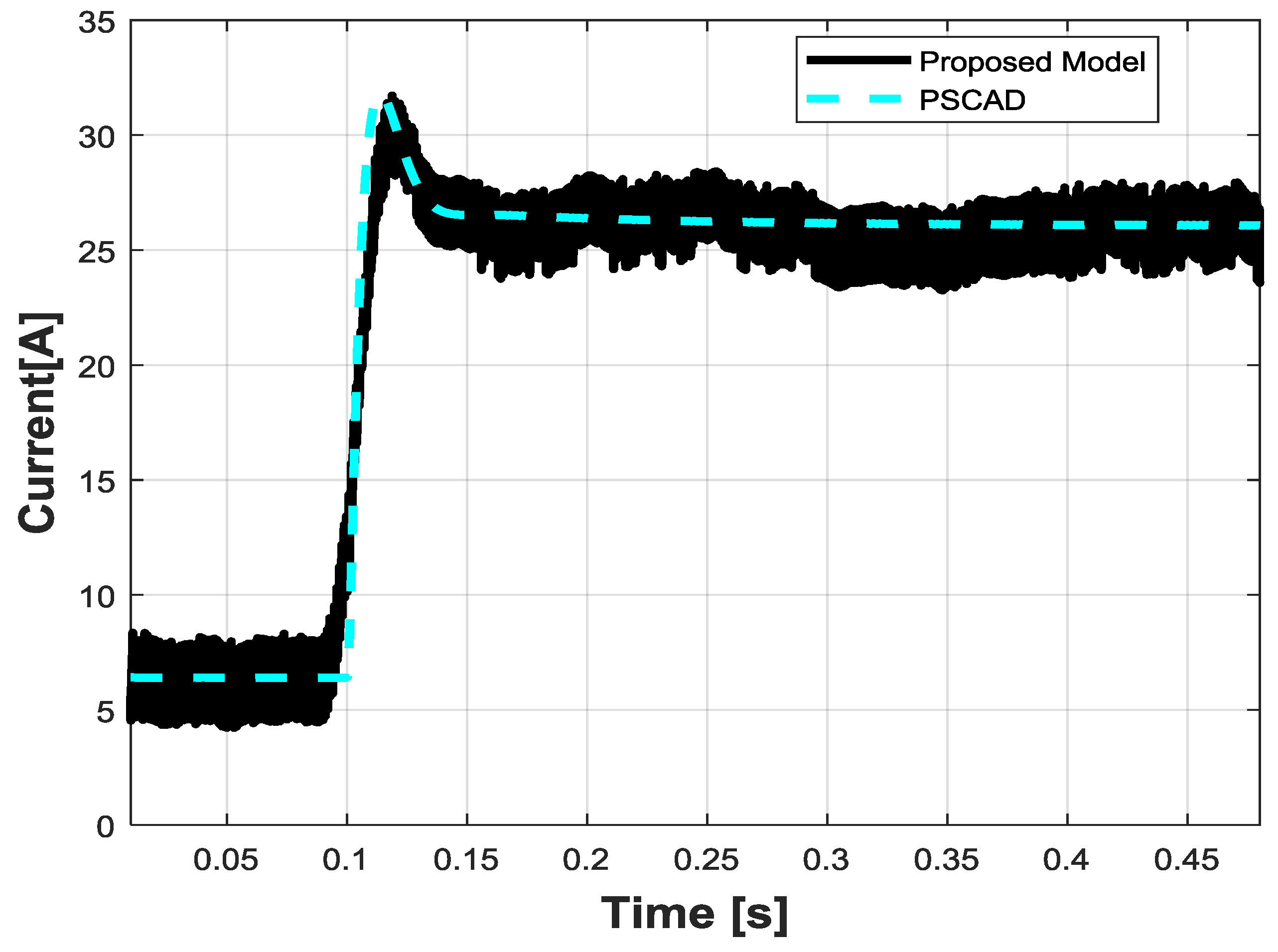
Figure 15.
Q2 bus voltage time profile for the load increasing scenario; the solid lines refer to PSCAD model while dashed ones refer to the proposed approach.
Figure 15.
Q2 bus voltage time profile for the load increasing scenario; the solid lines refer to PSCAD model while dashed ones refer to the proposed approach.
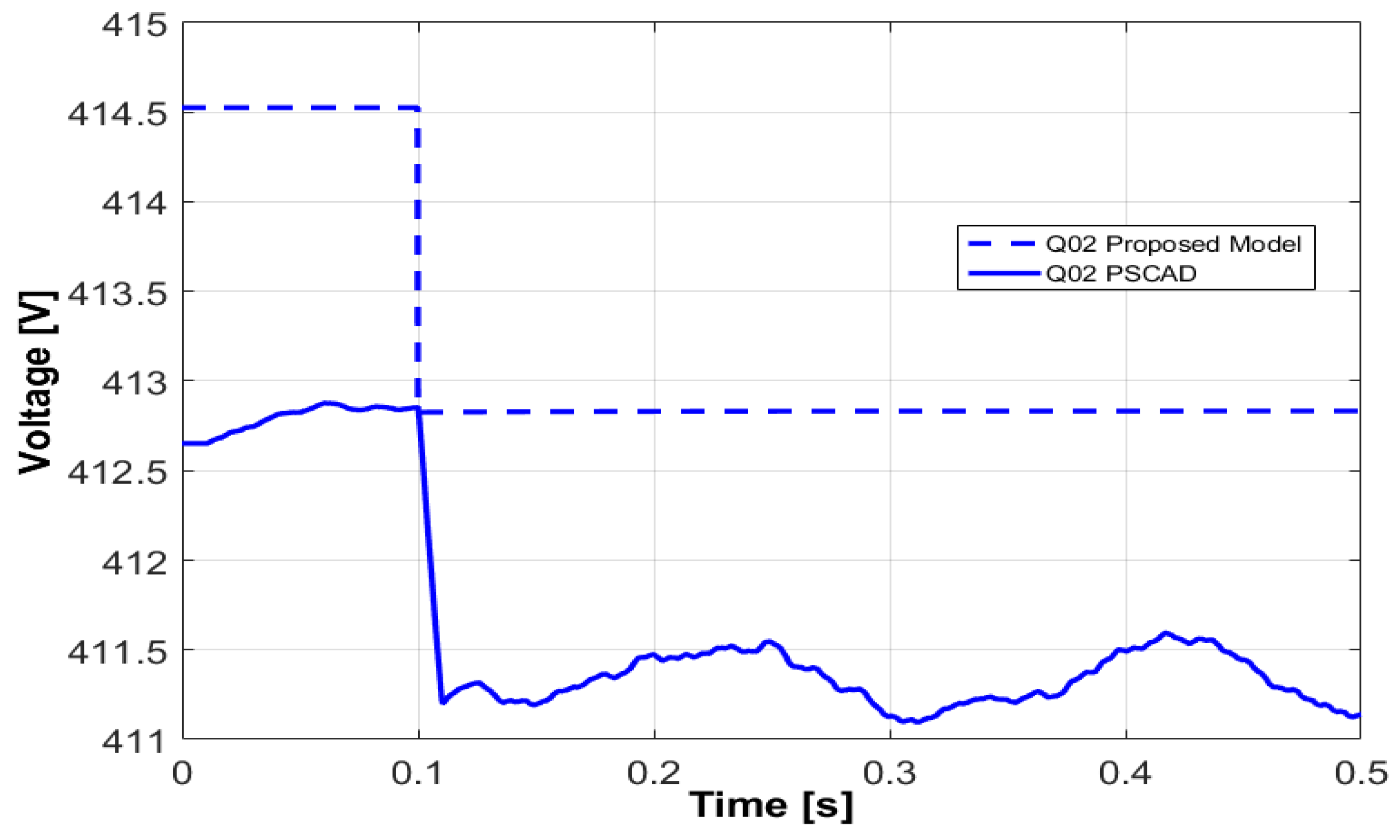
Figure 16.
Active power time profile for the load decreasing scenario; the solid line refers to PSCAD model while dashed ones refer to the proposed approach.
Figure 16.
Active power time profile for the load decreasing scenario; the solid line refers to PSCAD model while dashed ones refer to the proposed approach.

Figure 17.
Frequencies output time profile for the load decreasing scenario; the solid line refers to PSCAD model while dashed ones refer to the proposed approach.
Figure 17.
Frequencies output time profile for the load decreasing scenario; the solid line refers to PSCAD model while dashed ones refer to the proposed approach.

Figure 18.
Active power time profile for the load decreasing scenario; the solid line refers to PSCAD model while dashed ones refer to the proposed approach.
Figure 18.
Active power time profile for the load decreasing scenario; the solid line refers to PSCAD model while dashed ones refer to the proposed approach.

Figure 19.
LST current profile for the load decreasing scenario; the solid line refers to PSCAD model while dashed ones refer to the proposed approach.
Figure 19.
LST current profile for the load decreasing scenario; the solid line refers to PSCAD model while dashed ones refer to the proposed approach.

Figure 20.
Q2 bus voltage time profile for the load decreasing scenario; the solid line refers to PSCAD model while dashed ones refer to the proposed approach.
Figure 20.
Q2 bus voltage time profile for the load decreasing scenario; the solid line refers to PSCAD model while dashed ones refer to the proposed approach.
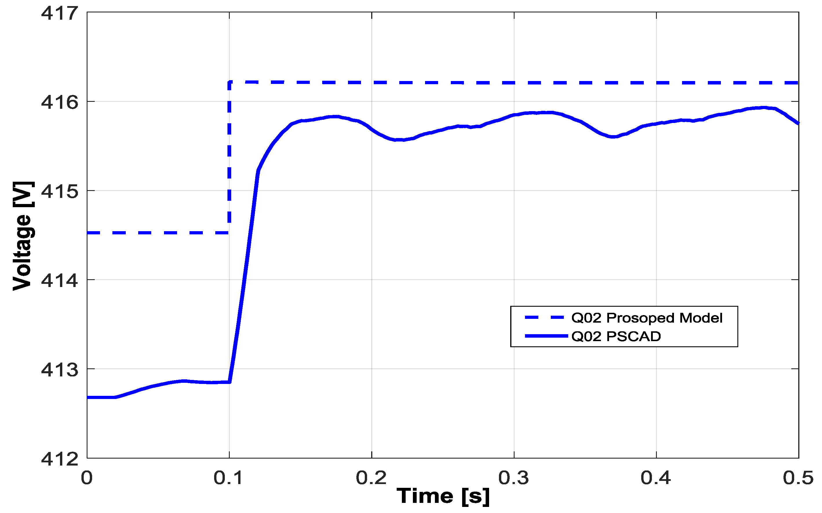
Figure 21.
Active power time profile for S3; the solid lines refer to PSCAD model while dashed ones refer to the proposed approach
Figure 21.
Active power time profile for S3; the solid lines refer to PSCAD model while dashed ones refer to the proposed approach
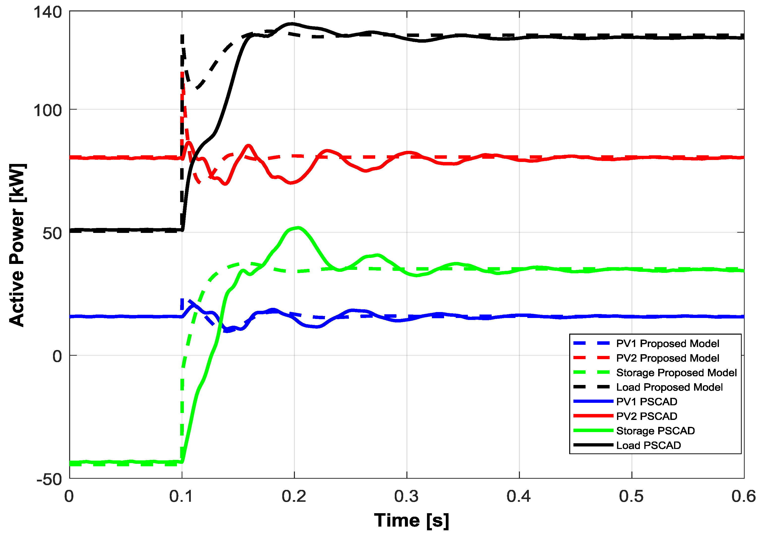
Figure 22.
DC capacitor voltage time profile for S3; the solid lines refer to PSCAD model while dashed ones refer to the proposed approach.
Figure 22.
DC capacitor voltage time profile for S3; the solid lines refer to PSCAD model while dashed ones refer to the proposed approach.

Figure 23.
LST current for S3; the solid lines refer to PSCAD model while dashed ones refer to the proposed approach.
Figure 23.
LST current for S3; the solid lines refer to PSCAD model while dashed ones refer to the proposed approach.
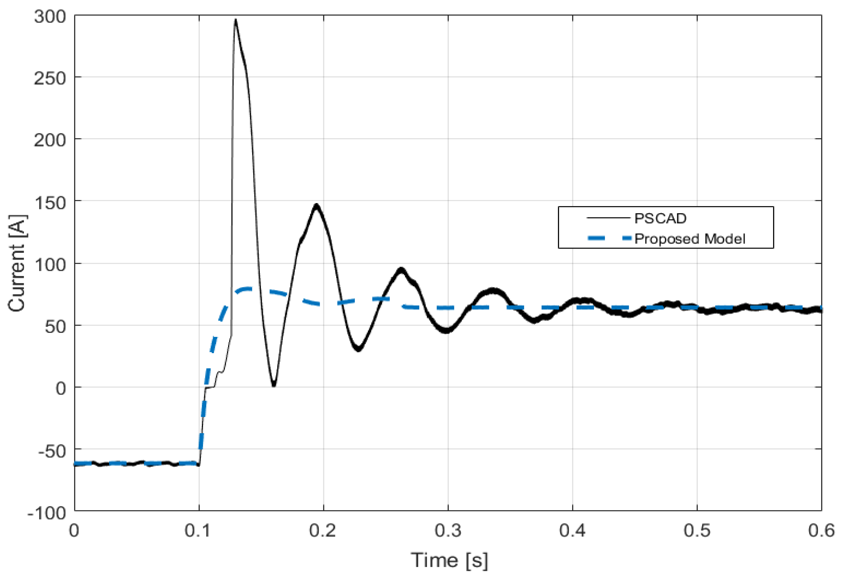
Figure 24.
Q2 bus voltage time profile for S3; the solid lines refer to PSCAD model while dashed ones refer to the proposed approach.
Figure 24.
Q2 bus voltage time profile for S3; the solid lines refer to PSCAD model while dashed ones refer to the proposed approach.
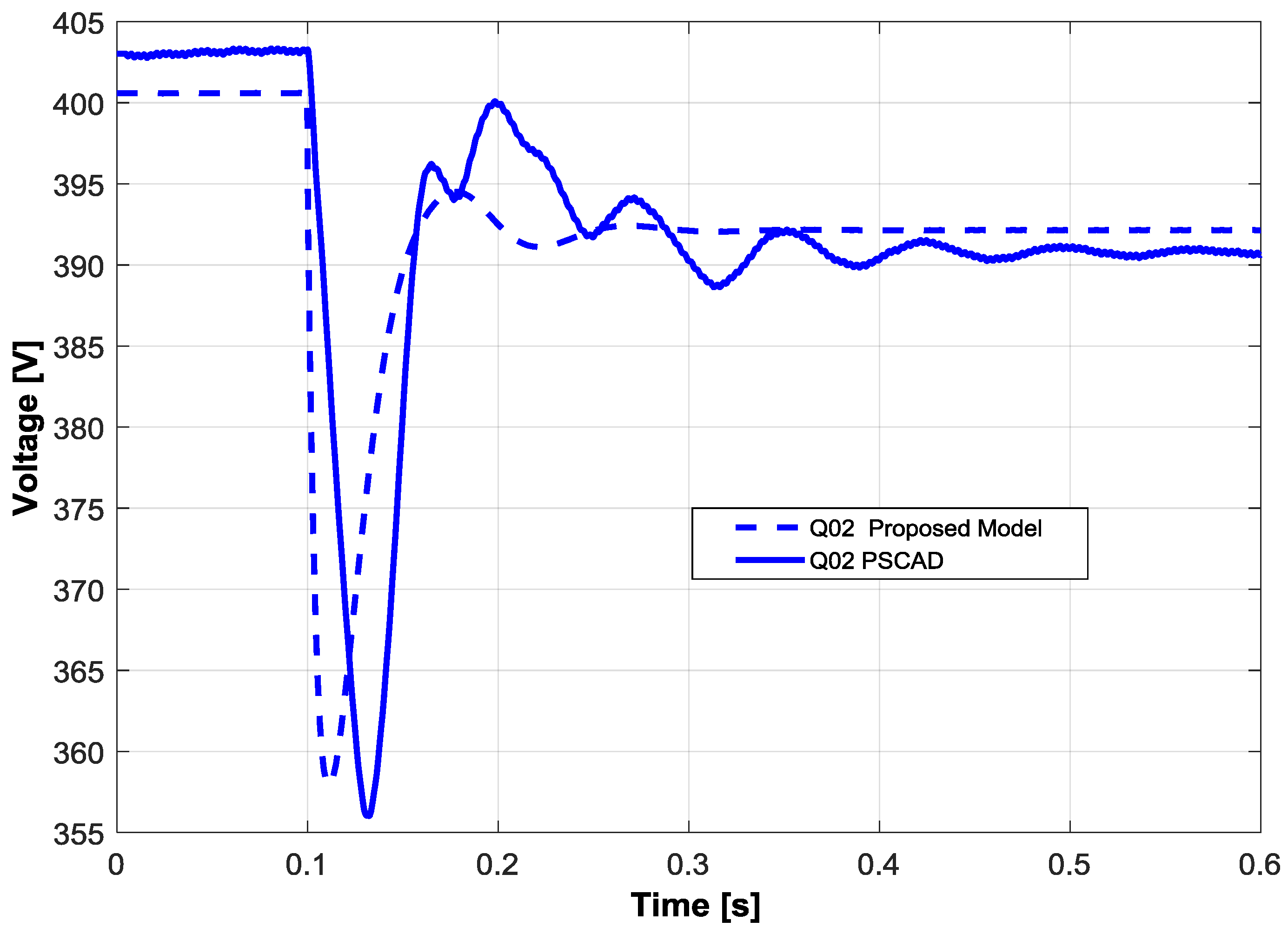
Figure 25.
Active power time profile for S4; the solid lines refer to PSCAD model while dashed ones refer to the proposed approach.
Figure 25.
Active power time profile for S4; the solid lines refer to PSCAD model while dashed ones refer to the proposed approach.
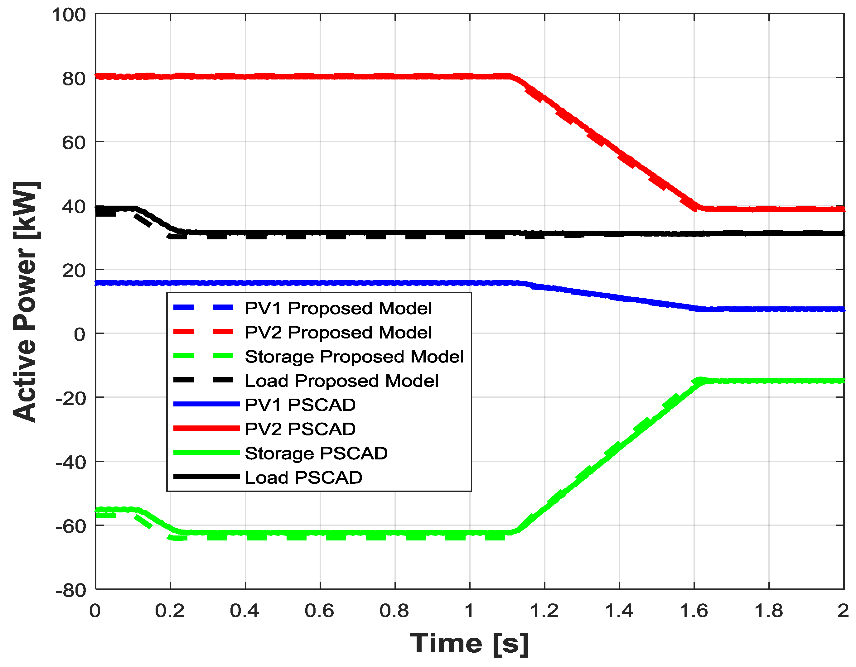
Figure 26.
DC capacitor voltage time profile for S4; solid lines refer to PSCAD model while dashed ones refer to the proposed approach.
Figure 26.
DC capacitor voltage time profile for S4; solid lines refer to PSCAD model while dashed ones refer to the proposed approach.

Figure 27.
Q2 bus voltage time profile for S4; the solid lines refer to PSCAD model while dashed ones refer to the proposed approach.
Figure 27.
Q2 bus voltage time profile for S4; the solid lines refer to PSCAD model while dashed ones refer to the proposed approach.

Figure 28.
LST current for S4; the solid lines refer to PSCAD model while dashed ones refer to the proposed approach.
Figure 28.
LST current for S4; the solid lines refer to PSCAD model while dashed ones refer to the proposed approach.


Table 1.
Sources data.
| Photovoltaic (PV) 1 | PV 2 | Storage | Load | |
|---|---|---|---|---|
| Rated Power | 3 × 5 kWp | 77 kWp | 62 kW | |
| Cable resistance to Q2 | 157.2 mΩ | 20.8 mΩ | 43.5 mΩ | 181 mΩ |
| Cable inductance to Q2 | 3023.7 μH | 14.15 μH | 12.42 μH | 14.59 μH |
Table 2.
PV Module parameters.
| PV Module Parameters | ||
|---|---|---|
| Short circuit current in Standard Test Conditions (STC) | 8.75 A | |
| Rated external temperature | 25 °C | |
| Temperature coeff. of the short circuit current | 0.06 | |
| Temperature coeff. of the open module voltage | −0.31 | |
| Minimum solar radiation to supply energy | 0.2 kW/m2 | |
| Maximum solar radiation to supply energy | 1 kW/m2 | |
| Open voltage module at | 35 V | |
| Open voltage module at | 37.11 V | |
| Maximum power point voltage in STC | VMPP | 29.7 V |
| Maximum power in STC | PMPP | 240 W |
Table 3.
Polynomial coefficients
| [A] | a6 | a5 | a4 | a3 | a2 | a1 | a0 |
|---|---|---|---|---|---|---|---|
| 0 [A] | 1.6 × 10⁻¹¹ | −4 × 10⁻⁹ | 6 × 10⁻⁷ | −3.3 × 10⁻⁵ | 7.5 × 10⁻⁴ | 5.2 × 10⁻⁴ | 2.42 |
Table 4.
AC filter parameters.
| Lse | Rse | Lsh | Csh | Rsh |
|---|---|---|---|---|
| 1 mH | 0.314 mΩ | 0.0166 mH | 1 µF | 2.61 kΩ |
Table 5.
DC/DC PI Parameters.
| Proportional Gain | Integral Time Constant | |
|---|---|---|
| Boost | KP_BOOST = 1.438 × 10⁻⁴ | TBOOST = 8.749 (s) |
| Buck | KP_BUCK = 1.667 × 10⁻⁴ | TBUCK = 10 (s) |
Table 6.
PVs inverter PI Parameters.
| Proportional Gain | Integral Time Constant | |
|---|---|---|
| phase | KP,phase = 5 × 10⁻⁴ | Tphase = 10 (s) |
| mod_index | KP,mod_index= 2 × 10⁻⁶ | Tmod_index= 2.5 103 (s) |
Table 7.
Droop parameters.
| PV1 | PV2 | Storage | |
|---|---|---|---|
| Pn | 15 kW | 77 kW | 62 kW |
| m | −1.000 × 10⁻⁴ rad/sW | −0.187 × 10⁻⁴ rad/sW | −0.242 × 10⁻⁴ rad/sW |
| Qn | 7.265 kVAr | 38.746 kVAr | 30.03 kVAr |
| n | −1.000 × 10⁻⁴ V/VAr | −0.187 × 10⁻⁴ V/VAr | −0.242 × 10⁻⁴ V/Var |
Table 8.
S1—Initial states.
| PV1 | PV2 | Storage | DC/DC Converter |
|---|---|---|---|
| VDC,1 = 783.8 V | VDC,2 = 854.8 V | VDC,3 = 750.0 V | χ1 = 0.153 |
| IST = 6.4 (A) | χ2 = 0.847 | ||
| SOC = 80% | |||
| ψ1 = 0.0524 rad | ψ2 = 0.0524 rad | ψ3 =0 rad | |
| φ1 = 0 | φ2 = 0 | φ3 = 0 |
Table 9.
S3—Initial states.
| PV1 | PV2 | Storage | DC/DC Converter |
|---|---|---|---|
| VDC,1 = 659.4 V | VDC,2 = 712.8 V | VDC,3 = 750.0 V | χ1 = 0.093 |
| η11 = 0.2234 | η12 = 0.2478 | IST = −66.5 A | χ2 = 0.907 |
| η21 = 1.01 | η22 = 0.94 | SOC = 10% | |
| ψ1 = 0 rad | ψ2 = 0 rad | ψ3 = 0 rad |
Table 10.
S4—Initial States.
| PV1 | PV2 | Storage | DC/DC Converter |
|---|---|---|---|
| VDC,1 = 659.4 V | VDC,2 = 712.8 V | VDC,3 = 750.0V | χ1 = 0.023 |
| η11 = 0.2595 | η12 = 0.2889 | IST = −72.07 A | χ2 = 0.977 |
| η21 = 0.99 | η22 = 0.90 | SOC = 80% | |
| ψ1 = 0 rad | ψ2 = 0 rad | ψ3 = 0 rad |
© 2017 by the authors. Licensee MDPI, Basel, Switzerland. This article is an open access article distributed under the terms and conditions of the Creative Commons Attribution (CC BY) license (http://creativecommons.org/licenses/by/4.0/).
Share and Cite
MDPI and ACS Style
Bonfiglio, A.; Brignone, M.; Invernizzi, M.; Labella, A.; Mestriner, D.; Procopio, R. A Simplified Microgrid Model for the Validation of Islanded Control Logics. Energies 2017, 10, 1141. https://doi.org/10.3390/en10081141
AMA Style
Bonfiglio A, Brignone M, Invernizzi M, Labella A, Mestriner D, Procopio R. A Simplified Microgrid Model for the Validation of Islanded Control Logics. Energies. 2017; 10(8):1141. https://doi.org/10.3390/en10081141
Chicago/Turabian StyleBonfiglio, Andrea, Massimo Brignone, Marco Invernizzi, Alessandro Labella, Daniele Mestriner, and Renato Procopio. 2017. "A Simplified Microgrid Model for the Validation of Islanded Control Logics" Energies 10, no. 8: 1141. https://doi.org/10.3390/en10081141
Note that from the first issue of 2016, this journal uses article numbers instead of page numbers. See further details here.