An Improved Method for Energy and Resource Assessment of Waves in Finite Water Depths


1
Centre for Marine and Renewable Energy Ireland, Environmental Research Institute, University College Cork, Cork P43 C573, Ireland
2
College of Mechanical and Energy Engineering, Jimei University, Xiamen 361021, China
*
Author to whom correspondence should be addressed.
Energies 2017, 10(8), 1188; https://doi.org/10.3390/en10081188
Submission received: 28 June 2017
/
Revised: 1 August 2017
/
Accepted: 9 August 2017
/
Published: 11 August 2017
Abstract
:For cost savings and ease of operation, nearshore regions have been considered as ideal regions for deploying wave energy converters (WECs) and wave farms. As the water depths of these regions may be frequently limited to 50 m or less, they can be considered as being transitional/intermediate to shallow when compared to the wave lengths of interest for wave energy conversion. Since the impact of water depths on propagation of waves is significant, it cannot be ignored in wave energy assessment. According to the basic wave theory, in order to work out accurate wave energy amounts in finite water depth, detailed wave spectral distributions should be given. However, for some practical reasons, there are still some cases where only scatter diagrams and/or the statistical wave parameters are available, whilst the detailed wave spectra are discarded. As a result, the assessments of wave energy and resources are frequently determined by ignoring the effect of water depths or using very simplified approximations. This research paper aims to develop more accurate approximation methods by utilising a number of available parameters such that a better estimate on the wave resource assessment can be achieved even if the detailed wave spectra are not available. As one important goal, the research can provide some important indications on how the measured wave data are effectively presented so that they can be very useful for assessing the wave energy resource, especially in the cases including the effects of finite water depths.
1. Introduction
Accurate assessment of the wave energy climate is very important for the reliable determination of WEC power performance and survivability. Most commonly the site assessment is based on either field measurements or numerical modelling or both. Large scale studies can either be on a global level providing information on the global wave energy resource and the distribution of wave energy [1,2,3,4], or on a regional level where national wave energy resources are assessed [5,6,7,8,9,10,11,12,13,14]. From such types of studies, the global offshore wave power is estimated at 32,000 TWh/year [2], and the availability of wave energy resources can vary significantly. In the northern hemisphere, the Atlantic Arc made up of the UK, Ireland, France, Spain and Portugal has the best wave resources, and thus attracts a lot of interest for wave energy production.
For commercial wave energy development, accurate and reliable measurements and assessments of the sea waves at the planned sites is critical for both the performance and survivability of the installed devices. With sufficient site data the detailed characteristics of the site in relation to the resource potential, extreme conditions as well as annual, seasonal and monthly trends can be determined [13]. Currently, nearshore and shallow water regions have been primarily examined for wave farm development due to their proximity to shore, shorter cable routes and generally lower development costs. Magagna et al. [15] collected information on current and proposed wave energy deployments and found that most of the installed wave energy converters have been deployed in water depths less than 50 m, and thus far, there are no deployments proposed where the water depth exceeds 100 m, so the water depths involved in the wave energy conversion should be regarded as being transitional/intermediate to shallow when compared to the wave lengths of interest for wave energy conversion, termed as ‘finite water depth’ for convenience in this research.
Water depth has a significant effect on the propagation of waves. Thus, in finite water depths, the effect of water depths on resource assessment becomes an important factor for accurate assessment of wave energy resources. It has been shown by Sheng and Li [16] that without water depth correction wave energy assessments could lead to errors of more than 10%. Conventionally, the effect of water depths on wave power could be easily considered if the detailed spectral distributions are available for analysis as seen when wave resource assessments [1,3,12,13,14,17,18,19] or the numerical models (such as the open source SWAN model [20,21]) are used [5,6,7,8,14].
However, in reality, there are still some cases that neither detailed wave spectra nor numerical models are available for wave energy resource assessment. For instance, for some confidential reasons, only some statistic parameters may be given instead of wave spectra, or for some economic reasons, there may be no numerical wave models available. In this regard, the wave energy assessments have been traditionally done either using the formula for deep water, by ignoring the effect of water depths [12,22] or using the simplified approximations to the water depth effect on wave energy calculations [1,14,16]. This paper aims to develop new approximation methods to improve the wave energy assessment in absence of detailed wave spectra or commercial wave models. In this research field, Cornett [1] suggests a constant wave group velocity calculated based on the wave energy period to approximate the effect of water depth. Recently, Sheng and Li [16] studied the approximation method and found that if the wave group velocity is calculated using the spectral peak period, the approximation may be more accurate and reliable, and as a result of the simple approximation, the error of the wave energy assessment can be reduced from more than 10% to less than 5% (Atan et al. [14] also suggest a formula using a single wave group velocity in the approximation, but no details are given on how the wave group velocity is calculated).
In this research, the new proposed methods are named as 3rd-order, 4th-order and 5th-order approximations, respectively. Compared to the zero-order approximation proposed by the authors in previous work [16], more available wave statistical periods, including the popular spectral peak period, energy period, mean spectral period and zero up-crossing period are used for the assessment. Because these statistic periods are calculated from the spectral moments of different orders, they contain different information from the spectrum distribution on frequencies to allow a more accurate approximation to the wave energy assessment. The proposed methods have been applied to the theoretical spectra (Bretschneider and JONSWAP) and the measured spectra on the Irish West Coast. The comparisons have shown that the new proposed approximation methods could reduce the errors for wave energy assessment to less than 1.5% (14% for the deep-water formulas) for individual sea states, and to less than 1% (10% for the deep-water formulas) for the overall wave resource.
The contents are arranged as follows: Section 2 gives the basic formula of the waves in finite water depths and the lower-order approximation method for wave energy in irregular waves; Section 3 gives the new approximation methods using more available wave statistic parameters; in Section 4, comparisons are made for the individual sea states for different theoretical spectra and the measured wave spectra. Relevant errors are calculated for illustrating the accuracy of the different approximation methods; Section 5 gives the comparisons on the overall wave resources calculated using different approximation methods in accordance with the wave scatter diagrams. Finally, the conclusions are given in Section 6.
2. Waves in Finite Water Depths
2.1. Wavelength in Finite Water Depth
From linear wave theory (the details can be found in [23,24,25]), in finite water depths the dispersion relation is given as:
where ω is the wave circular frequency, h the water depth, k the wave number, given by k = 2π/λ, with λ being the wavelength.
Based on the dispersion relation (1), the wavelength in finite water depth, h, can be solved using the following equation:
where λ0 (=gT2/2π) is the wavelength in deep water (the subscript ‘0’ indicates the parameter in deep water hereafter).
2.2. Approximations for Wave Energy Calculation
In the cases of finite water depths, the wave energy is dependent on the spectrum (spectral distribution) and the frequency-dependent modification coefficient Ch for a given water depth (noted as Ch(ω) hereafter). The generic wave energy (wave power) equation is given by (see [16]):
with Ch defined as:
It can be seen that the modification is water depth dependent, see Figure 1. Hence, to calculate the wave energy accurately using Equation (3), the modification coefficient Ch (which is only wave frequency dependent for a given water depth) must be determined for the corresponding spectral components. There have been some research work carried out on spectral models for waves in finite depths [26,27]. Given the detailed spectrum, an accurate calculation of wave energy can be carried out using Equation (3).
2.2.1. Deep Water Conditions
In deep water where k0h > 3.14 (that is, h/λ0>1/2), Ch is almost a constant (named Ch0 = 1.0). Thus the wave energy in such condition for a given sea state is calculated as:
where can be calculated from the spectral moment (defined as below) when n = −1.
2.2.2. Spectral Moments
The nth-order spectral moment is calculated by:
where n is an integer. For ocean waves, the most used moments are n = −2, −1, 0, 1, 2, corresponding to the spectral moments noted as m−2, m−1, m0, m1 and m2. These spectral moments are used to define the useful wave statistic parameters. Also, for the proposed method for improving the wave energy and resources assessment these spectral moments will be used.
2.2.3. Wave Statistics
In the cases when these wave statistical parameters are given, the wave spectral moments can be calculated as follows:
Using Equations (8) and (9) could yield the other spectral moments:
2.3. Zero-Order Modification Method
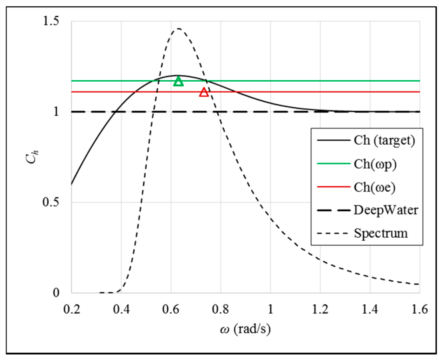
Sheng and Li [16] considered the effect of finite water depth on the wave energy calculation by assuming that the modification factor Ch is a constant (thus named the zero-order approximation). The basic assumption for the method is that the actual wave powers/spectra concentrated on a limit bandwidth. For instance, for a Bretschneider spectrum (Tp = 8 s, Hs = 2.0 m), 50% of the energy is concentrated within a bandwidth of 0.305 rad/s around the peak period [16]. Hence it may be reasonable to suggest that Ch can be approximated with a constant value. However, as Ch(ω) is frequency-dependent it can be varied by using different frequency or period (named as wave characteristic frequency ωc or characteristic period Tc). The calculated spectral peak period Tp and the energy period Te of the given sea state are the common used characteristic periods. Figure 2 shows the comparison of the zero-order modifications for the given sea state, Tp = 10 s (Hm0 = 2.0 m) and the water depth 25 m. From the plot, it can be obtained that Ch(ωp) = 1.17 and Ch(ωe) = 1.11. When these two modification coefficients are used in Equation (3), the wave energy is actually increased by 17% and 11% respectively when compared to the case without correction (i.e., Ch0 = 1.0). The formula for a constant Ch is written as:
where ωc is the wave characteristic frequency.
As described in [16], using the constant Ch(ωp) or Ch(ωe) as the modification coefficient (as seen in Figure 2) can favourably improve the accuracy of the wave energy assessment. The maximal error for the zero-order method happens when Ch(ωp) or Ch(ωe) is at the peak of the Ch curve, at which the correction factor may contribute to over-estimate the integration, but it is still much more accurate than that of using Ch0. As already shown in [16], the use of the deep-water formula could underestimate the wave energy by 13%, and with the zero-order approximation, the maximal error could reduce to 5% for individual sea state. Using the spectral peak period or energy period may give different errors in different conditions, but both are within 5% (Figure 3a,b).
3. New Methods of Approximations
3.1. Approximations to the Modification Coefficient Ch
To calculate the wave energy more accurately in the cases of finite water depths, it is important to reproduce Ch to the real Ch curve as accurate as possible for the given water depth (shown in Figure 3). In this research, more accurate methods are proposed using more parameters available for the wave energy and resources assessment. To more accurately reproduce the modification function Ch, different order polynomial functions can be used. For instance, the 3rd-order polynomial function is given as:
where the coefficients a1, a2 and a3 of the polynomial function can be obtained using the least square method to fit the calculated Ch in a given frequency range. It should be noted that the 3rd-polynomial function can only reproduce Ch very accurately in a relative narrow bandwidth, for instance, 0.5ωe–1.25ωe (see Figure 4a).
Similarly, we can use 4th- or 5th-order polynomial function, as:
Similarly, the coefficients bi (i = 1,…, 4) and cj (j = 1,…, 5) can be obtained using the least squares method for a given frequency range if the better reproduction of Ch is required. For the higher polynomial functions, better reproduction results of Ch can be seen in a wider range of frequencies: the 4th-order method reproduces Ch well for frequency range of 0.5ωe–1.67ωe for which range the 3rd-order approximation is not so good (see Figure 4b). The 5th-order method is good for even a larger frequency range of 0.5ωe–2.5ωe which could cover most of the wave spectrum. For comparison, the 3rd- and 4th-order methods do not produce a good result (see Figure 4c).
In these figures, the spectra are also plotted for reference, and from these figures it can be seen that the higher order approximation can cover a larger range of the frequencies for the spectrum, thus it can produce much improved predictions for wave energy with the effects of finite water depths.
3.2. Wave Energy Approximations Methods
Using the proposed approximation formulas for the modification coefficient Ch, the wave energy for a given sea state can be calculated.
3.2.1. 3rd-Order Method
Based on the 3rd-order polynomial approximation for Ch, the wave energy is calculated as:
where a1, a2 and a3 are the 3rd-order polynomial function coefficients in Equation (12), and m−1, m0 and m1 the nth order spectral moments for n = −1, 0 and 1, which can be calculated using the significant wave height, the energy period and the spectral mean period, via Equations (9) and (10).
3.2.2. 4th-Order Method
Using the 4th-order polynomial approximation for Ch, the wave energy for the given sea state is given as:
One more moment m2 is used than the 3rd-order method, and this moment can be obtained using the wave statistical period, T02, the zero upcrossing period (Equation (10)).
3.2.3. 5th-Order Method
Using the 5th-order polynomial approximation to Ch, the wave energy can be calculated as:
From the above approximations, it can be seen that the spectral moments from n = −2 to n = 2 are used, and these moments are actually those which have been conventionally used to define the statistical parameters of the ocean waves, including the significant wave height and the statistic periods in Equations (7) and (8). Alternatively if the wave statistical parameters are given, the spectral moments can be obtained using Equations (9) and (10).
It should be noted that a polynomial function with a higher order can give better approximations to Ch, with the higher order moments of the wave spectrum being invoked accordingly. However, in practice spectral moments of higher order than 2 are not commonly used so the highest polynomial approximation in this research has an order of 5, see Equations (14) and (17).
4. Wave Energy Assessment in Finite Water Depths
In this section, the wave energies for different sea states in finite water depths are calculated using the method described in previous sections and the results are compared to the ‘Accurate’ value as determined from real or theoretical spectral data using Equation (3). The result figures also show the zero-order result with the reference frequency, the energy frequency of the spectrum, ωe (regarded as ‘Zero-order’ in the figures) and the uncorrected wave energy (‘DeepWater’ in the figures). In the figures, the results from the 3rd-order, 4th-order and 5th-order methods are all plotted (identified as ‘3rd-order’, ‘4th-order’ and ‘5th-order’, respectively). The errors in percentage are given by the following formula:
where Eapprox is the wave energy calculation using different approximation methods, and Eaccur is the wave energy using the accurate integral via Equation (3).
4.1. Bretschneider Spectra (Hm0 = 2 m for All Cases)
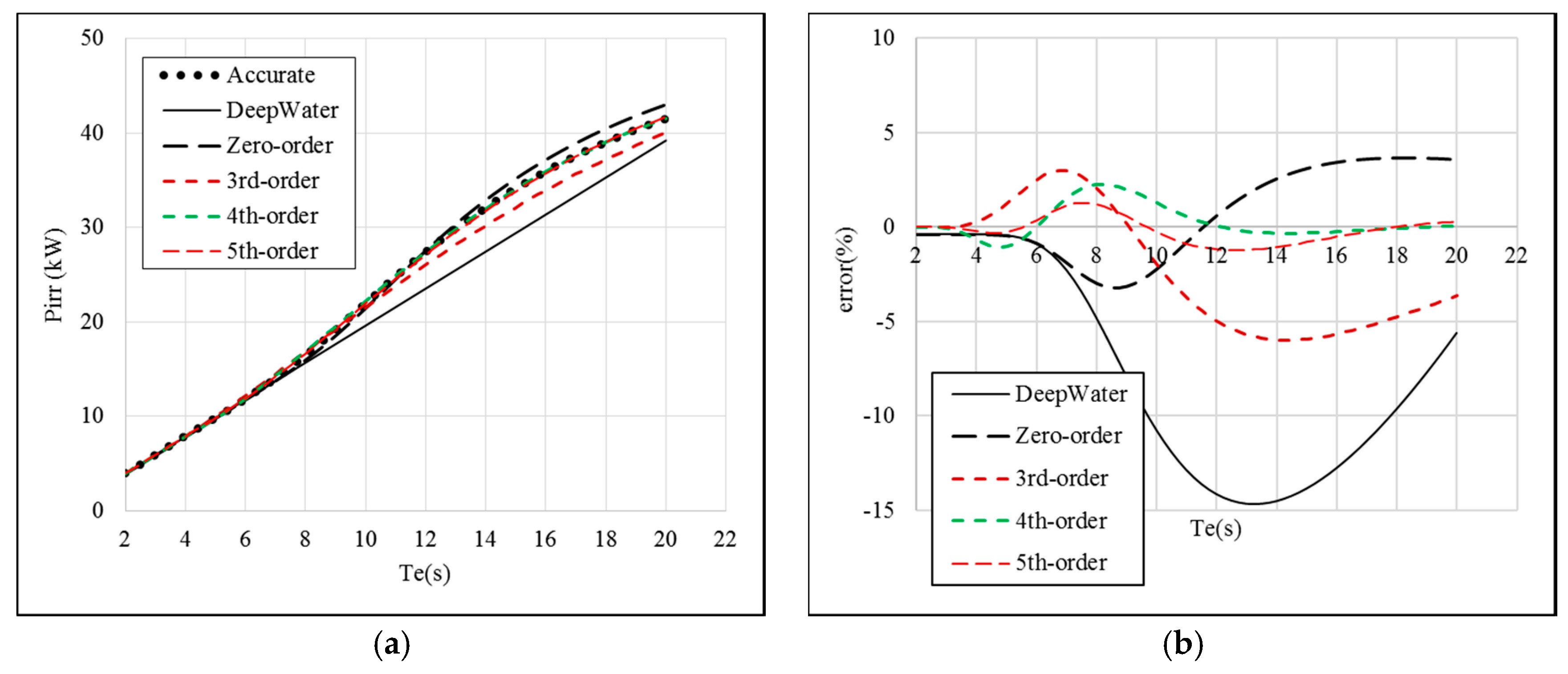
Figure 5a shows the comparison of the wave energy calculations and corresponding errors using different correction methods in the case of water depth = 50 m. It can be seen that for the small wave periods (Te < 6.0 s), the water depth of 50 m would be taken as that of deep water condition, thus the corrections could be small. For longer waves, the deep water condition can underestimate the wave energy assessment by as much as 13% (see Figure 5b). The zero-order correction with the peak period underestimates the wave power for waves in the 6–10.5 s range, and then overestimates the wave power for the wave energy periods between 10.5 s and 20 s, with a maximal error just greater than 5%. The 3rd-order approximation gives an opposite trend to the zero-order method, with a maximal error of about 5%, while the 4th and 5th-order method have maximal errors of only 1.5% and 1% respectively.
In the case of water depth of 25 m, it can be seen from Figure 6a that the deep water condition consistently gives underestimations for wave periods (Te < 15 s) with a maximal error of 13%. Again, the zero-order and the 3rd-order method give similar error range, but with opposite trends, the corresponding maximal errors by these two methods are about 5%. Again the 4th-order and 5th-order approximations give much more accurate calculation of wave energy, with maximal errors of 1.5% and 1% respectively (see Figure 6b).
4.2. Standard JONSWAP Spectra (Hm0 = 2 m for All Cases)
In the cases of the standard JONSWAP spectra, it can be seen from Figure 7 and Figure 8 that similar results are obtained for the cases of Bretschneider spectra, but there are the following differences:
- (1)
- The deep water condition gives underestimations of the wave power with a maximal error being about 14.5%;
- (2)
- The correction using the zero-order method is better than the 3rd-order method, with a slightly smaller maximal error (3.5% vs. 6%).
- (3)
- The 4th-order and 5th-order methods are very good approximations, with maximal errors being 2.5% and 1.5% respectively for the 25 m and 50 m water depths.
4.3. Measured Waves at AMETS
In the following analysis, wave spectra from the Atlantic Marine Energy Test Site (AMETS) (Belmullet, Ireland) in the 50 m water depth are analysed. The wave measurements are same to those used by Cahill et al. [13] with a 13,189 individual measurements available in 2010. The data were recorded by two wave buoys, with an overall availability about 75% (the detailed availability of the data can be seen in [13]). These measured spectra are used in the following analysis and comparison.
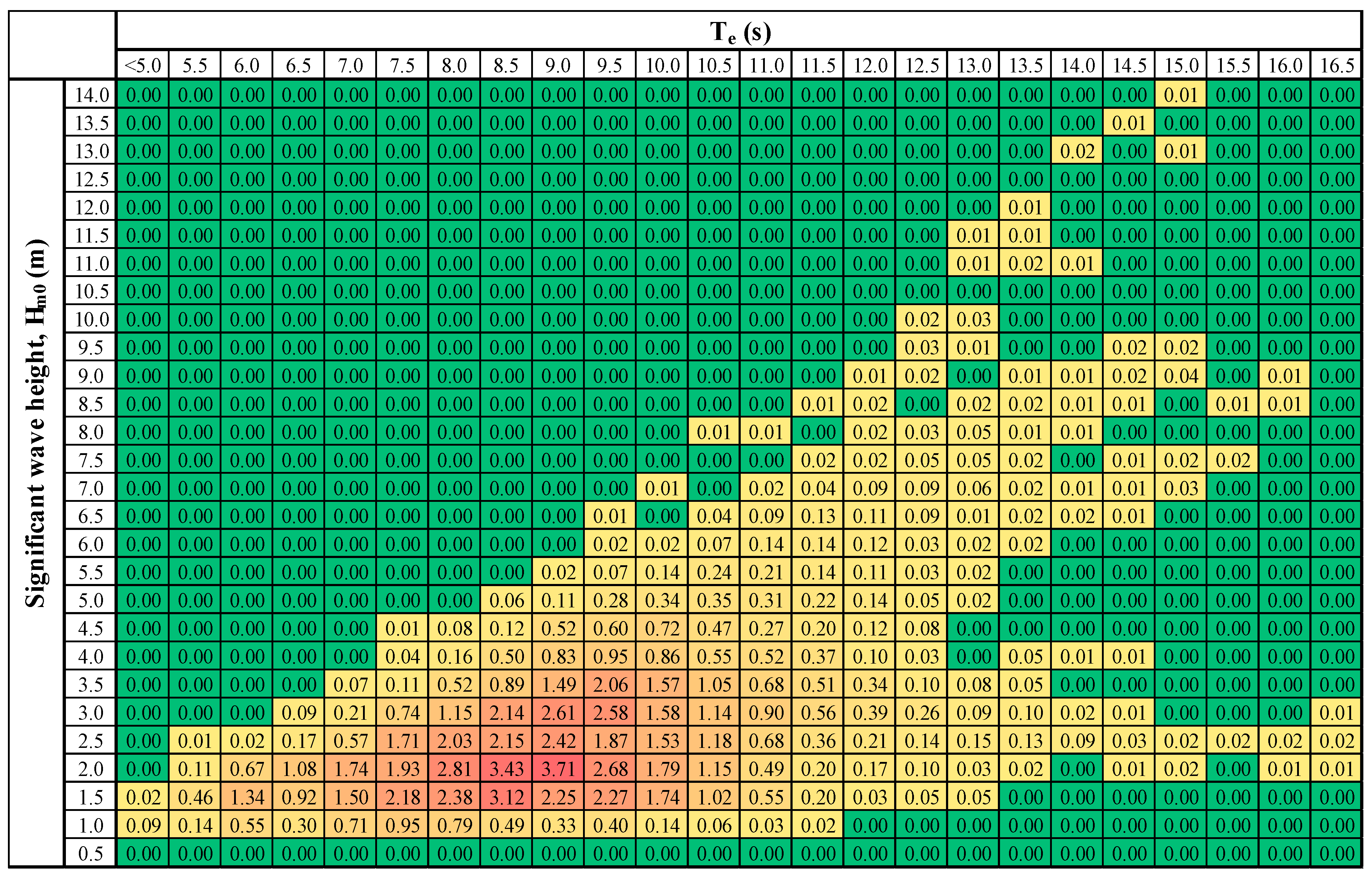
Using the measured wave heights Hm0 and energy period, Te, these wave statistics are binned/grouped using the bins corresponding to the given significant wave heights (Hm0 = 0–0.5 m, 0.5–1.0 m, 1.0–1.5 m,… using 0.5 m bin sizes) and the corresponding reference energy periods (Te < 5.0 s, 5.0–5.5 s, 5.5–6.0 s,… using a bin size of 0.5 s) and a wave scatter diagram can be built (see Figure 9). Meanwhile those spectra grouped in one bin are averaged to represent the corresponding wave spectrum for the given bin for comparison. For each bin, the significant wave height and the energy period can be taken directly from the scatter diagram at the mid values of a particular bin or they can be calculated from the average spectrum in the bin. In addition, for the proposed approximation methods in this research, other statistical wave periods are also assumed to be available, such as the calculated spectral peak period, Tpc, spectral mean period, T01, and the zero upcrossing period, T02, because the 5th-order approximation uses all these parameters.
Also from the available measured spectra, the direct integrals for all measured spectra can be accurately calculated using Equation (3), and the results can be regarded as the accurate wave energy (‘Accurate’ in the figure).
4.3.1. Measured Spectra
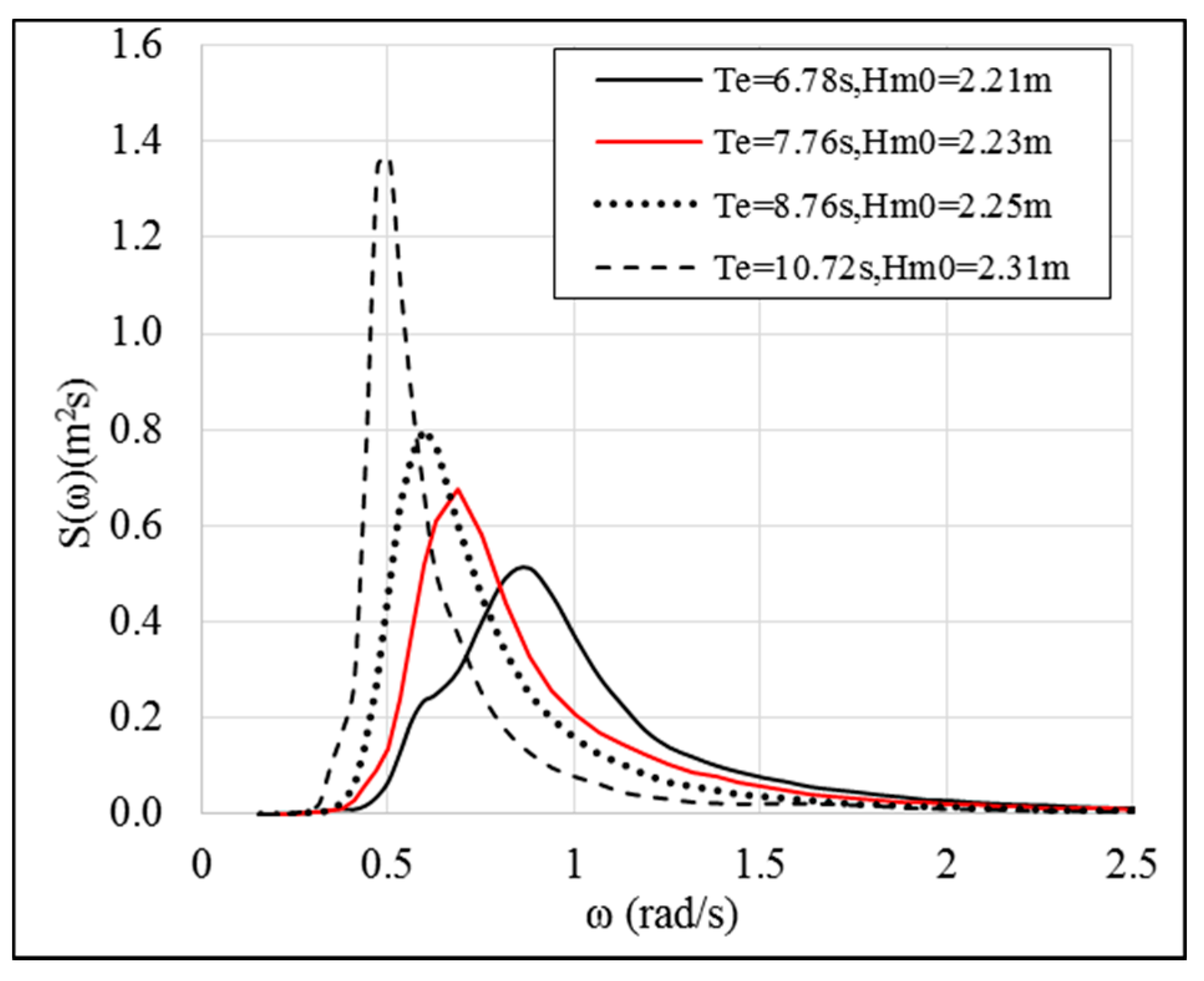
Figure 10 shows four different measured spectra for four bins in the wave scatter diagram, with the average significant wave heights and energy periods: Hm0 = 2.21 m and Te = 6.78 s; Hm0 = 2.23 m and Te = 7.76 s, Hm0 = 2.25 m and Te = 8.76 s and Hm0 = 2.31 m and Te = 10.72 s. Though the actual significant wave heights and the energy periods are slightly different from those from the scatter diagram i.e., Hm0 = 2.25 m and Te = 6.75 s; Hm0 = 2.25 m and Te = 7.75 s; Hm0 = 2.25 m and Te = 8.75 s and Hm0 = 2.25 m and Te = 10.75 s. Very small differences can be only found for these two methods.
In Figure 11, the measured spectrum is compared to the corresponding Bretschneider and JONSWAP spectra. Obviously, the measured wave spectrum differs from the conventional Bretschneider (‘gamma’, γ = 1.0) and JONSWAP (γ = 3.3) spectra, but agrees with the JONSWAP spectrum with γ = 1.5. For such a single peak spectrum, the calculated spectral peak period works very well. It is also worth to mentioning that to reproduce the measured spectrum using the generalised JONSWAP spectrum, the different spectral peakness γ may be necessary.
4.3.2. Wave Energy Assessments
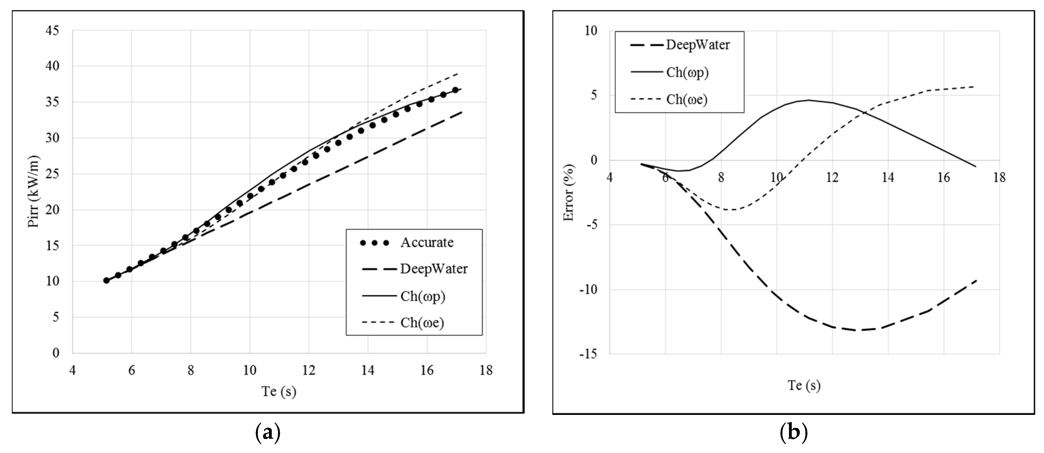
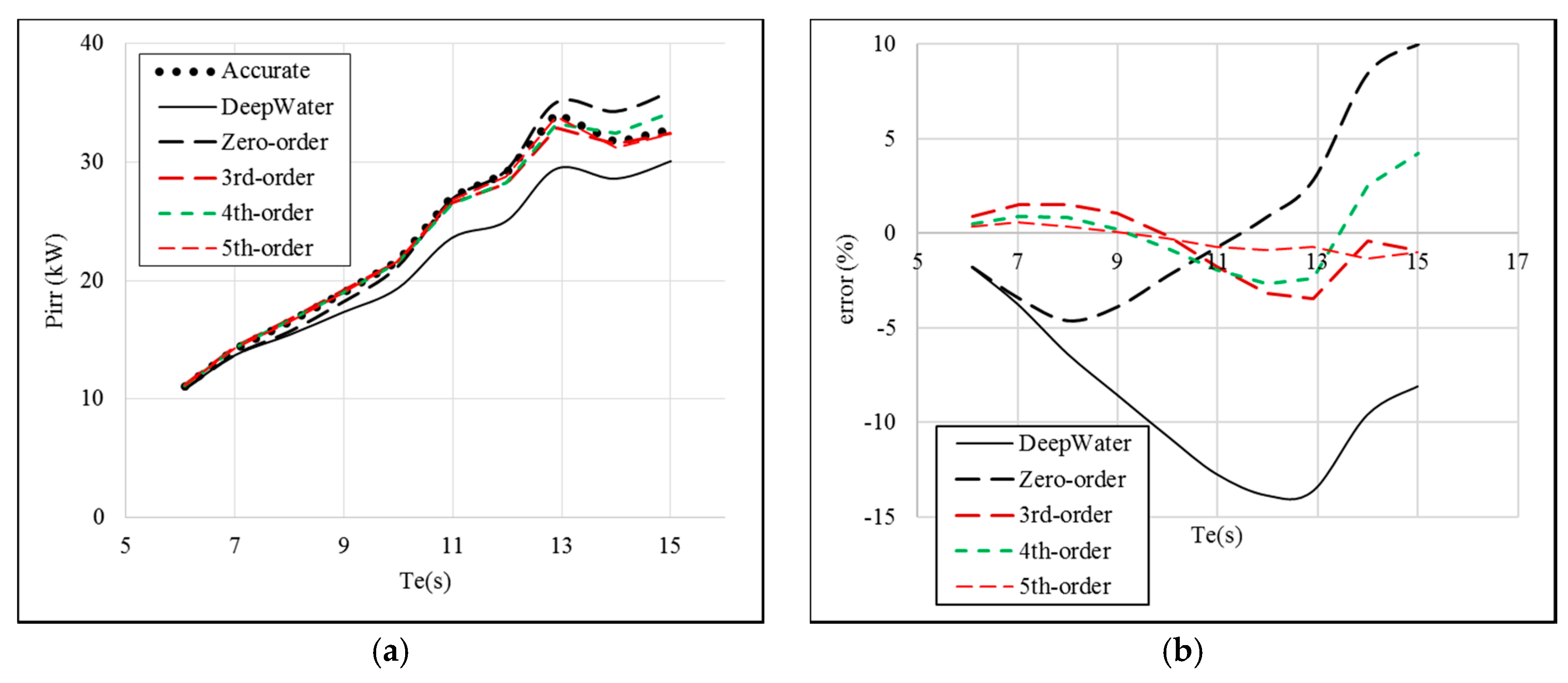
Figure 12 shows a comparison of the different corrections for the wave power assessment in a 50 m water depth. It can be seen that the deep-water formulas under-estimate the wave power for all wave periods, and the maximal error is about 14%. The zero-order approximation has an under-estimation of 5% at Te = 8 s, and a large over-estimation, with an error up to 10% for the long waves Te = 15 s.
The 3rd-order, 4th-order and 5th-order approximations all give better wave energy calculations, and for most waves, the maximal errors are smaller than 3%. It is noted that the largest error for the 3rd-order method happens at wave periods between 11 s and 13 s.
5. Results and Analysis
Scatter diagrams are used for assessing the wave energy resources. In Figure 9, the scatter diagram has a bin size of 0.5 m on significant wave height and 0.5 s on the energy period (termed ‘0.5 m and 0.5 s’ hereafter). This has been followed the IEC TS 62600-101 technical specification [26], in which the bin size of the scatter diagram is required to be smaller than 0.5 m and 1.0 s. However, for the purpose of analysis, larger bin sizes are used for comparison in this section. Regardless of the bin size in the diagram, the significant wave height and the energy period for each bin are taken as the mid-values of the bin, which in fact may be slightly different from those directly calculated from the average spectrum for the bin. But other parameters used in the approximation methods, including the spectral peak period, mean spectral period and the mean upcrossing period, are directly calculated using the average spectrum for the bin.
5.1. Bin Size and Wave Energy Assessment
In the first case, the accuracy of the different approximation methods on the assessment are examined for both the binned spectra and the individual spectra. Table 1 shows the results from the 3rd-order, 4th-order and 5th-order methods. For comparison, the results using the deepwater condition and the zero-order methods using ωe and ωp are also listed.
From Table 1, the very small differences can be found for the binned (average) spectra and the direct calculation from all individual spectra (see the last column in Table 1). However, different approximation methods give some different results: the deep-water formula gives an under-estimation between 10% and 11% for the annual mean wave power for both water depths (50 m and 25 m) whilst the zero-order correction methods based on the spectral peak and energy periods give the error between −1.0% and 4.0%. Generally speaking, the 3-order and 4th-order correction methods have a similar accuracy to the zero-order method, and the 5th−order correction shows the most accurate approximation, with the errors being less than 1% in all cases.
The analysis also shows that there are minimal differences between the results from the individual spectra and the binned average spectra. It was found that bin size has a small effect on the wave energy assessment (Table 2), until very large sized bin is used. In particular, the accurate wave energy calculation whether using the individual spectra or the binned average spectra, the results are always same, which can be proven as follows.
The accurate wave energy (average on all sea states) is given:
A manipulation on above equation yields:
This is a proof that the average of all the wave energy power for all sea states equals to the wave power when using the average spectrum. Hence it can be seen that the bin size will not have an effect on the accurate wave energy calculation.
It must be pointed out that the same principle can be extended to the significant wave height, Hm0, but not other parameters. This is why when the bin size is very large, for instance, 2.0 m and 2.0 s, all the approximation methods give increased errors when compared to those using same approximation method with smaller bin size.
5.2. Scatter Diagram and Wave Energy Assessment
In applying the proposed methodology it is assumed that the scatter diagram is available along with other statistical wave periods, such as T01, T02 and Tpc. In this study, the significant wave height and energy period are taken as the mid-value for the bin, which is different from the above analysis, in which the significant wave height and energy period are calculated from the averaged spectra in the bin.
By employing the methods proposed in this research, the results from the 3rd-order, 4th-order and 5th-order methods are all listed in Table 3. From the table, it can be seen that the deep-water formula gives an under-estimation between 9% and 11% for the annual mean wave power for both water depths. The zero-order correction methods based on the spectral peak and energy periods give the errors between −1.0% and 5% for both water depths. Again, the accuracies can vary a lot for both zero-order corrections on the water depths.
The 3-order and 4th-order correction methods have shown slightly better results than the zero-order method. In both water depths, the 5th-order correction shows the best approximation, with the errors being less than 1% in all cases. Again, for this specific bin size, the errors between the individual spectra and the scatter diagram are very small for the same approximation methods.
By increasing the bin size, the errors may increase accordingly, see Table 4. To the maximum bin size specified by the IEC TS 62600-101 [26], the errors are still quite small. However, further increasing the bin size, larger errors can be seen. In particular, a very large increase in the error can be seen for the zero-order approximation method with ωp. The reason for this large change may be that the large bins could group the wind-generated waves and the swells, and for which the calculated peak period may not be a very good parameters for reference.
6. Conclusions
To more accurately assess the wave energy assessment at finite water depths, a method is proposed that uses scatter diagrams and some other statistical wave periods, including Tp, T01 and T02. From the analyses and comparisons, the proposed method is capable of significantly improving the accuracy of the assessment of wave energy resource. From the study, following conclusions can be drawn:
- (1)
- The examples using the theoretical spectra (Bretschneider and JONSWAP) have shown that the proposed method can significantly improve the assessment accuracy of wave energy calculation at finite water depths, reducing the maximal error from about 14% to less than 1.0% for the individual wave state for the 5th-order method, with the 3rd-order and 4th-order methods presenting slightly better and more reliable results than the zero-order method.
- (2)
- The proposed 5th-order method can considerably improve the assessment of the annual mean wave power for the measured sea waves, with a maximal error less than 1.0% for the AMETS data. In comparison, the deep water formulas give an error between 9.5% and 11% under-estimation, and the zero-order method gives a maximal error about 4.5%. The 3rd-order and 4th-order methods give more reliable results than the zero-order method.
- (3)
- Bin size in the scatter diagram may be important for assessing the wave resources. From the example in the study, the maximum bin size allowed by the IEC TS 62600-101 seems appropriate for guaranteeing very accurate assessment of wave energy and resources.
- (4)
- Based on the proposed method, the 5th-order method gives very consistently accurate wave energy calculation. For employing the 5th-order approximation method, the relevant parameters must be provided. Hence to make the wave data more useful, it is suggested that in addition to the scatter diagram (from which the significant wave height, Hm0 and energy period, Te can be decided), the calculated spectral peak period, Tp, spectral mean period T01 and zero upcrossing period T02 are ideally provided.
- (5)
- Other statistical parameters (if available) can also be used for further improving the assessment of the wave energy in finite water depths. For instance, in shipbuilding industry and research, the wave peak to peak period, T24 (=) is often suggested ([27]). Such additional parameter (parameters) could allow higher-order approximation (more than 5th-order) and thus better and more accurate assessments can be expected.
Acknowledgments
The first author would like to thank Science Foundation Ireland (SFI) Centre for Marine and Renewable Energy Research (MaREI) (Grant No. 12/RC/2302), Environmental Research Institute, University College Cork for providing funding support. The second author would like to thank the National Natural Science Foundation of China (Grant No. 51409118) for the finance support of the research work. The authors would like to acknowledge Brendan Cahill (Sustainable Energy Authority Ireland, SEAI) for providing the wave spectra for the analysis in this study.
Author Contributions
Wanan Sheng planned and formulated the research work, and checked the calculated results and wrote the manuscript. Hui Li coded the programs & carried out the main calculation and revised the manuscript. Jimmy Murphy helped to fund for Wanan Sheng and revised the manuscript extensively to improve both the technical terms and the language in the paper.
Conflicts of Interest
The authors declare no conflict of interest.
References
- Cornett, A. A global wave energy resource assessment. In Proceedings of the International Offshore and Polar Engineering Conference, Vancouver, BC, Canada, 6–11 July 2008. [Google Scholar]
- Mork, G.; Barstow, S.F.; Kabuth, A.; Teresa Pontes, M. Assessing the global wave energy potential. In Proceedings of the OMAE2010 29th International Conference on Ocean, Offshore Mechanics and Arctic Engineering, Shanghai, China, 6–11 June 2010. [Google Scholar]
- Gunn, K.; Stock-Williams, C. Quantifying the global wave power resource. Renew. Energy 2012, 44, 296–304. [Google Scholar] [CrossRef]
- Arinaga, R.A.; Cheung, K.F. Atlas of global wave energy from 10 years of reanalysis and hindcast data. Renew. Energy 2012, 39, 49–64. [Google Scholar] [CrossRef]
- Iglesias, G.; Lopez, M.; Carballo, R.; Castro, A.; Fraguela, J.; Frigaard, P. Wave energy potential in galicia (nw spain). Renew. Energy 2009, 34, 2323–2333. [Google Scholar] [CrossRef]
- Iglesias, G.; Carballo, R. Wave energy and nearshore hot spots: The case of the se bay of biscay. Renew. Energy 2010, 35, 490–500. [Google Scholar] [CrossRef]
- Rusu, L.; Guedes Soares, C. Wave energy assessments in the azores islands. Renew. Energy 2012, 45, 183–196. [Google Scholar] [CrossRef]
- Rusu, L. Assessment of the wave energy in the black sea based on a 15-year hindcast with data assimilation. Energies 2015, 8, 10370–10388. [Google Scholar] [CrossRef]
- Reikard, G.; Robertson, B.; Buckham, B.; Bidlot, J.-R.; Hiles, C. Simulating and forecasting ocean wave energy in western canada. Ocean Eng. 2015, 103, 223–236. [Google Scholar] [CrossRef]
- Lenee-Bluhm, P.; Paasch, R.; Ozkan-Haller, H.T. Characterizing the wave energy resource of the us pacific northwest. Renew. Energy 2011, 36, 2106–2119. [Google Scholar] [CrossRef]
- Hughes, M.G.; Heap, A.D. National-scale wave energy resource assessment for australia. Renew. Energy 2010, 35, 1783–1791. [Google Scholar] [CrossRef]
- Dufour, G.; Michard, B.; Cosquer, E.; Feragu, E. Emacop project: Assessment of wave energy resource along france’s coastlines. In Proceedings of the Coasts, Marine Structures and Breakwaters 2013, Edinburgh, UK, 18–20 September 2013. [Google Scholar]
- Cahill, B.G.; Lewis, A. Wave energy resource characteristion of the altantic marine energy test site. Int. J. Mar. Energy 2013, 1, 3–15. [Google Scholar] [CrossRef]
- Atan, R.; Goggins, J.; Nash, S. A detailed assessment of the wave energy resource at the atlantic marine energy test site. Energies 2016, 9, 967. [Google Scholar] [CrossRef]
- Magagna, D.; Uihleih, A. Ocean energy development in europe: Current status and future perspectives. Int. J. Mar. Energy 2015, 11, 84–104. [Google Scholar] [CrossRef]
- Sheng, W.; Li, H. A Method for Energy and Resource Assessment of Waves in Finite Water Depths. Energies 2017, 10, 460. [Google Scholar] [CrossRef]
- Forrest, S. A methodology for nearshore wave resource assessment. In Proceedings of the International Conference on Ocean Energy, Bilbao, Spain, 6–8 October 2010. [Google Scholar]
- Folley, M.; Whittaker, T. Analysis of the nearshore wave energy resource. Renew. Energy 2009, 34, 1709–1715. [Google Scholar] [CrossRef]
- Folley, M. The wave energy resource. In Handbook of Ocean Wave Energy; Pecher, A., Kofoed, J.P., Eds.; SpringerOpen: London, UK, 2017; Volume 7. [Google Scholar]
- Booij, N.; Ris, R.C.; Holthuijsen, L.H. Third-generation wave model for coastal regions 1. Model description and validation. J. Geophys. Res. 1999, 104, 7649–7666. [Google Scholar] [CrossRef]
- Ris, R.C.; Holthuijsen, L.H.; Booij, N. A third-generation wave model for coastal regions, 2. Verification. J. Geophys. Res. 1999, 104, 7667–7681. [Google Scholar] [CrossRef]
- Reguero, B.G.; Vidal, C.; Menendez, M.; Mendez, F.J.; Minguez, R.; Losada, I. Evaluation of global wave energy resource. In Proceedings of the IEEE Oceans 2011, Santander, Spain, 6–9 June 2011. [Google Scholar]
- Holthuijsen, L.H. Waves in Oceanic and Coastal Waters; Cambridge University Press: Cambridge, UK, 2007. [Google Scholar]
- Newman, J.N. Marine Hydrodynamics; The MIT Press: Cambridge, MA, USA, 1977. [Google Scholar]
- Tucker, M.J.; Pitt, E.G. Waves in Ocean Engineering; Elsevier Science Ltd.: Oxford, UK, 2001. [Google Scholar]
- International Electrotechnical Commission. Marine Energy-Wave, Tidal and Other Water Current Converters- Part 101: Wave Energy Resource Assessment and Characterization; IEC TS 62600–101; International Electrotechnical Commission: London, UK, 2015. [Google Scholar]
- Stansberg, C.T.; Contento, G.; Hong, S.W.; Irani, M.; Ishida, S.; Mercier, R.M.; Wang, Y.; Wolfram, J. The specialist committee on waves: Final report and recommendations to the 23rd ITTC (International Towing Tank Conference). In Proceedings of the 23rd International Towing Tank Conference, Venice, Italy, 8–14 September 2002. [Google Scholar]
Figure 1.
Modification coefficient Ch.
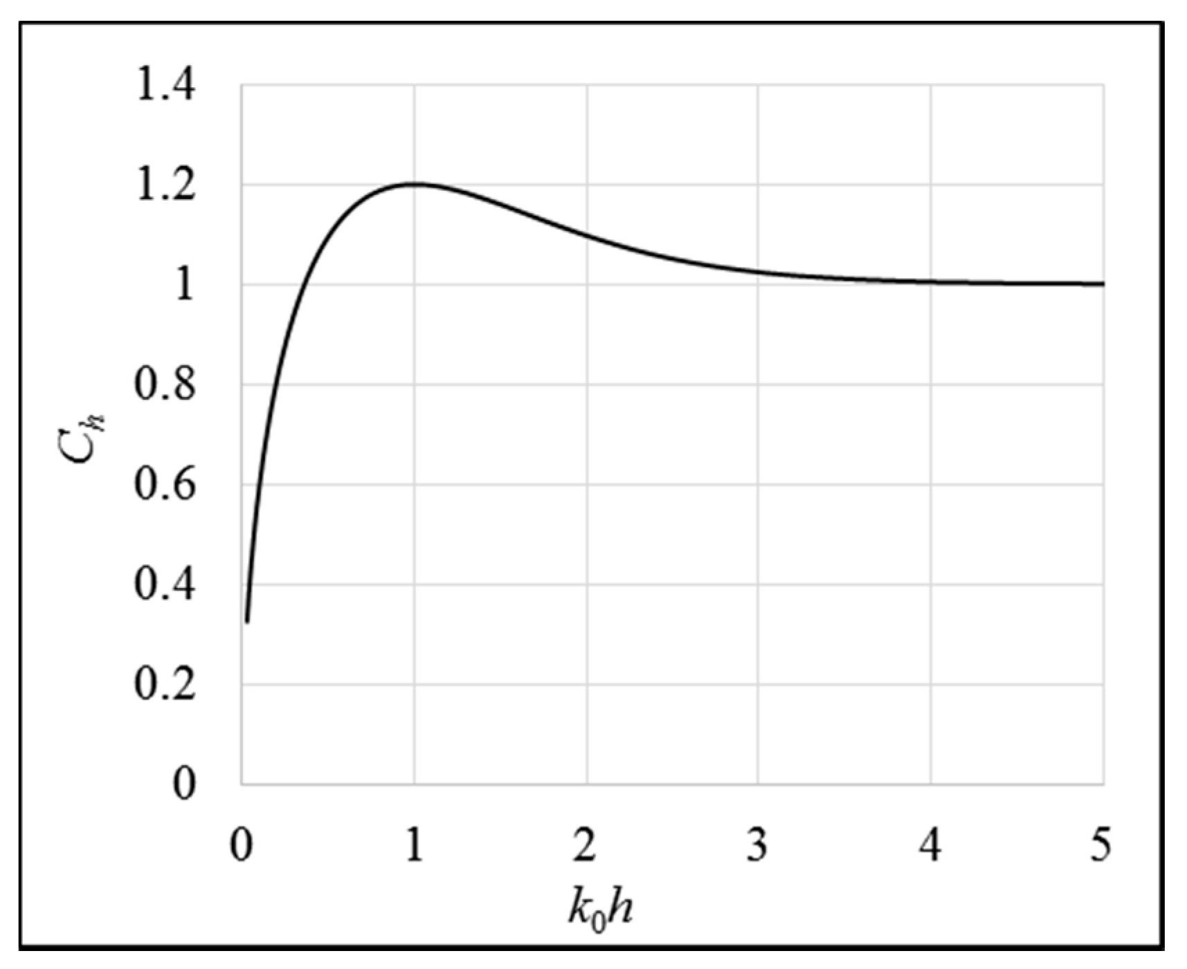
Figure 2.
Comparison of the zero-order modifications and the deepwater formula. Case: h = 25 m, Tp = 10 s.
Figure 2.
Comparison of the zero-order modifications and the deepwater formula. Case: h = 25 m, Tp = 10 s.

Figure 3.
Comparison of the calculated wave power and the corresponding error by zero-order modifications against the accurate calculation and the deepwater condition (Case: h = 25 m, Tp = 10 s). (a) Calculated wave power; (b) Error.
Figure 3.
Comparison of the calculated wave power and the corresponding error by zero-order modifications against the accurate calculation and the deepwater condition (Case: h = 25 m, Tp = 10 s). (a) Calculated wave power; (b) Error.

Figure 4.
Ch approximations for different frequency ranges (note: Te = 2π/ωe is the wave energy period). (a) 0.5ωe–1.25ωe; (b) 0.5ωe–1.67ωe; (c) 0.5ωe–2.5ωe.
Figure 4.
Ch approximations for different frequency ranges (note: Te = 2π/ωe is the wave energy period). (a) 0.5ωe–1.25ωe; (b) 0.5ωe–1.67ωe; (c) 0.5ωe–2.5ωe.
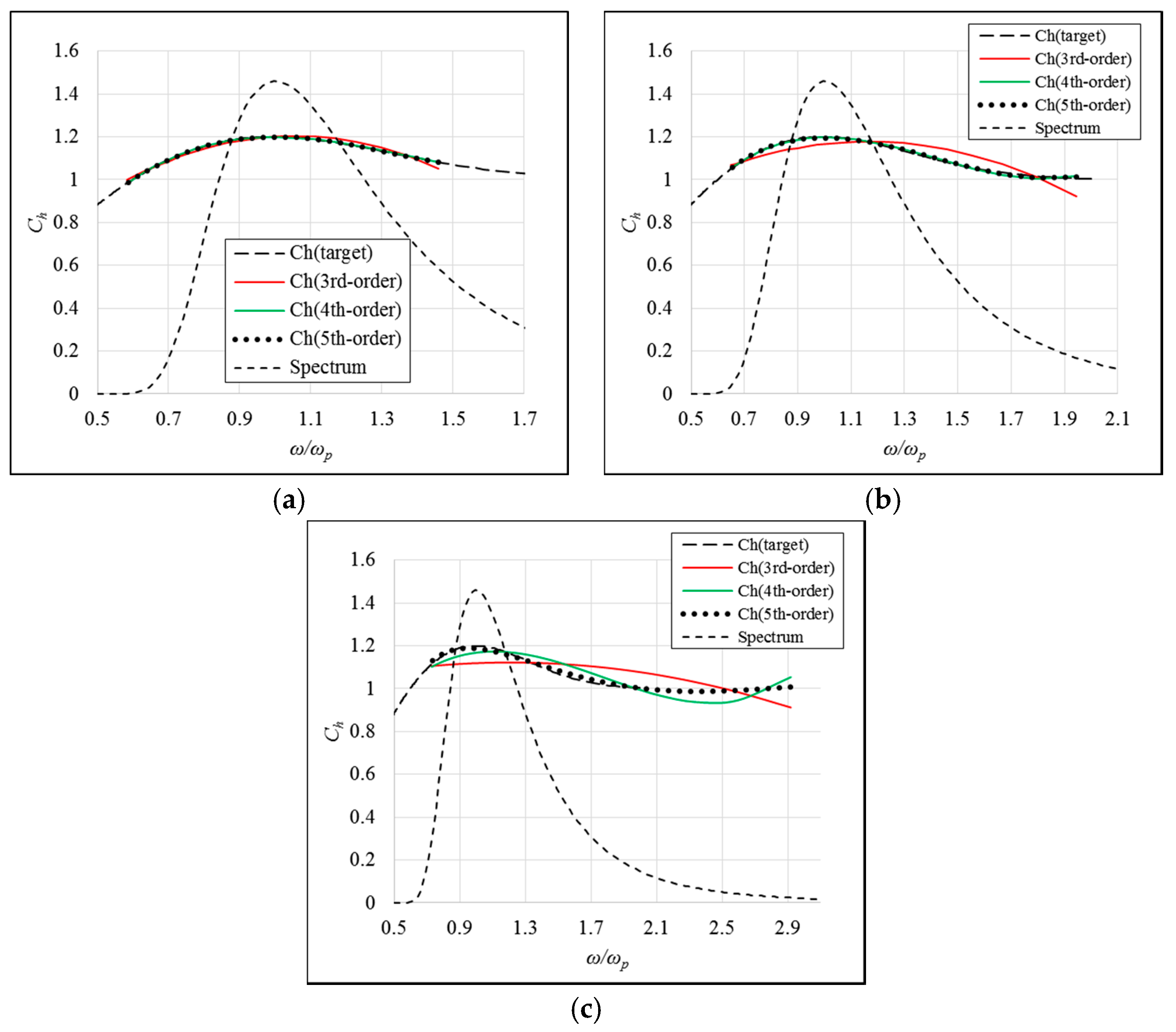
Figure 5.
Comparison of the calculated wave power and the corresponding error using different methods for Bretschneider spectra of Hm0 = 2 m (water depth = 50 m). (a) Calculated wave power; (b) Error.
Figure 5.
Comparison of the calculated wave power and the corresponding error using different methods for Bretschneider spectra of Hm0 = 2 m (water depth = 50 m). (a) Calculated wave power; (b) Error.
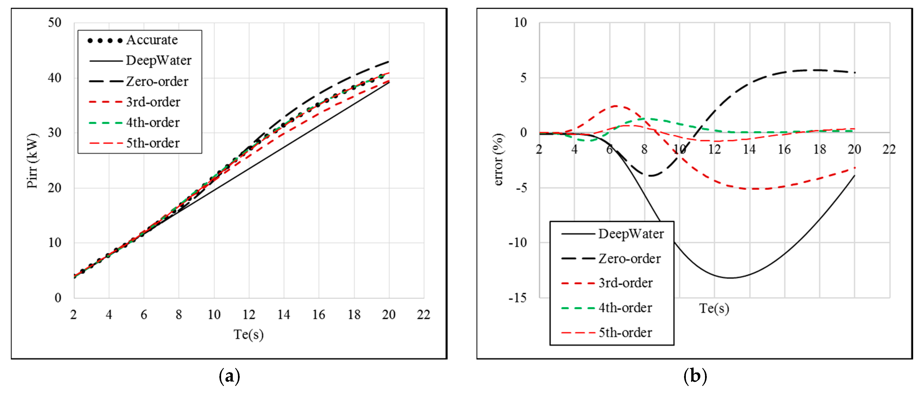
Figure 6.
Comparison of the calculated wave power and the corresponding error using different methods for Bretschneider spectra of Hm0 = 2 m (water depth = 25 m). (a) Calculated wave power; (b) Error.
Figure 6.
Comparison of the calculated wave power and the corresponding error using different methods for Bretschneider spectra of Hm0 = 2 m (water depth = 25 m). (a) Calculated wave power; (b) Error.
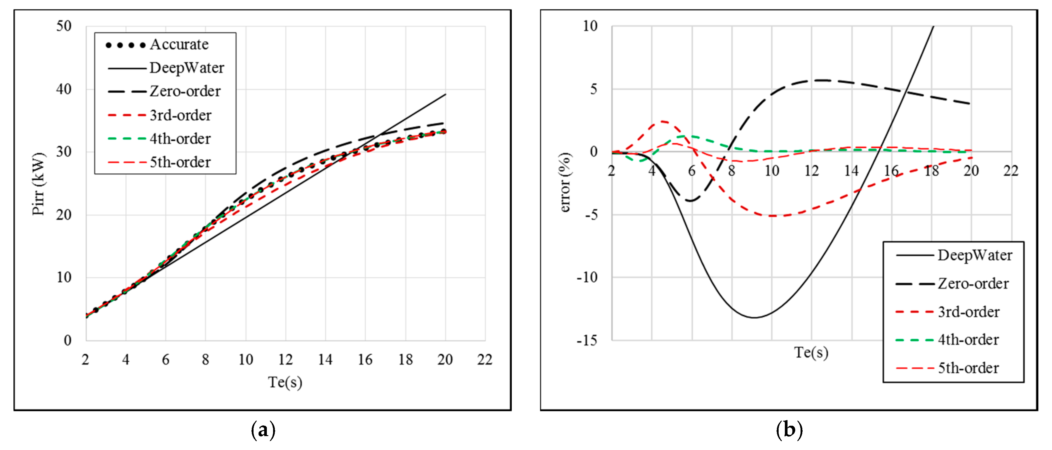
Figure 7.
Comparison of the calculated wave power and the corresponding error using different methods for JONSWAP spectra of Hm0 = 2 m (water depth = 50 m). (a) Calculated wave power; (b) Error.
Figure 7.
Comparison of the calculated wave power and the corresponding error using different methods for JONSWAP spectra of Hm0 = 2 m (water depth = 50 m). (a) Calculated wave power; (b) Error.

Figure 8.
Comparison of the calculated wave power and the corresponding error using different methods for JONSWAP spectra of Hm0 = 2 m (water depth = 25 m). (a) Calculated wave power; (b) Error.
Figure 8.
Comparison of the calculated wave power and the corresponding error using different methods for JONSWAP spectra of Hm0 = 2 m (water depth = 25 m). (a) Calculated wave power; (b) Error.
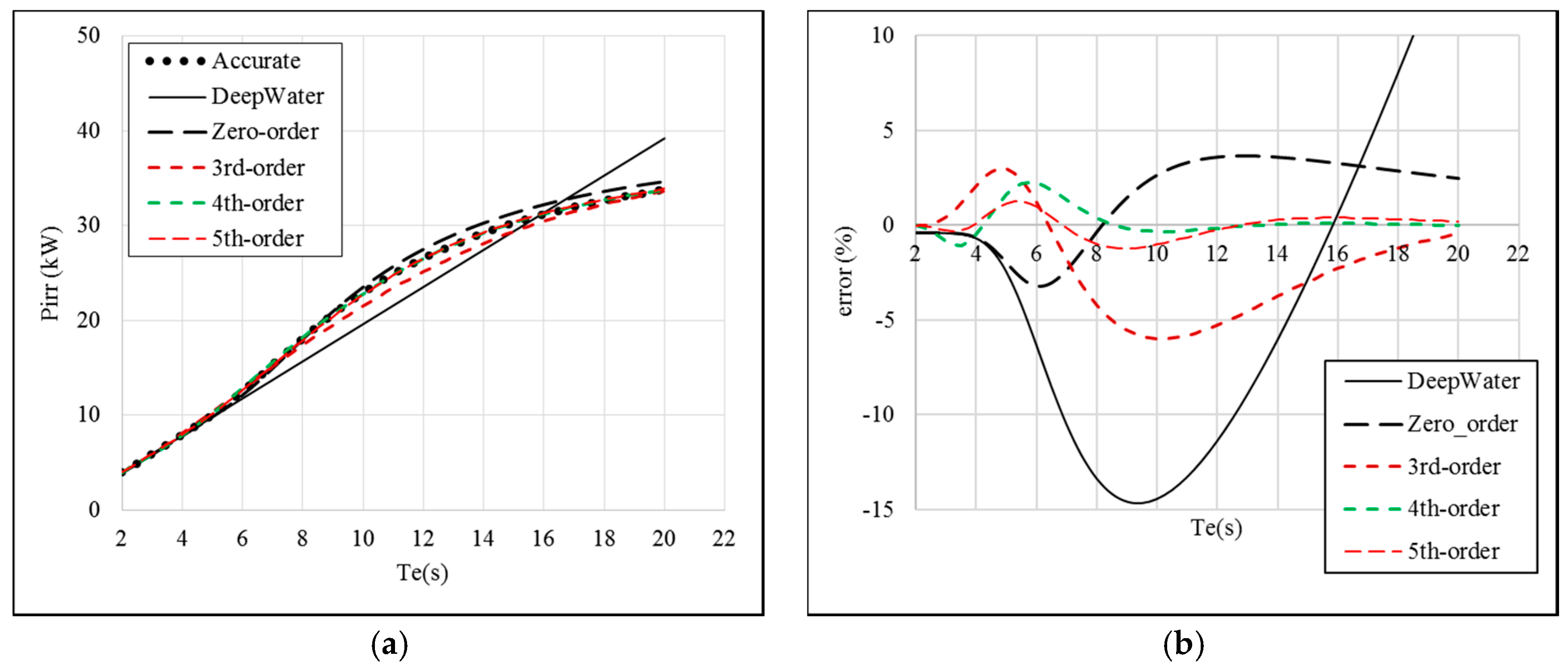
Figure 9.
Scatter diagram of the waves in AMETS in 2010 (available data points 13189 for two wave buoys, 75% availability).
Figure 9.
Scatter diagram of the waves in AMETS in 2010 (available data points 13189 for two wave buoys, 75% availability).

Figure 10.
Average measured wave spectrum for 4 different average periods (Hm0 ≈ 2.25 m).

Figure 11.
Measured spectrum (average) and the corresponding Bretschneider and JONSWAP spectra (Hm0 = 2.25 m, Te = 9.75 s), Tpc is calculated using Equation (8).
Figure 11.
Measured spectrum (average) and the corresponding Bretschneider and JONSWAP spectra (Hm0 = 2.25 m, Te = 9.75 s), Tpc is calculated using Equation (8).
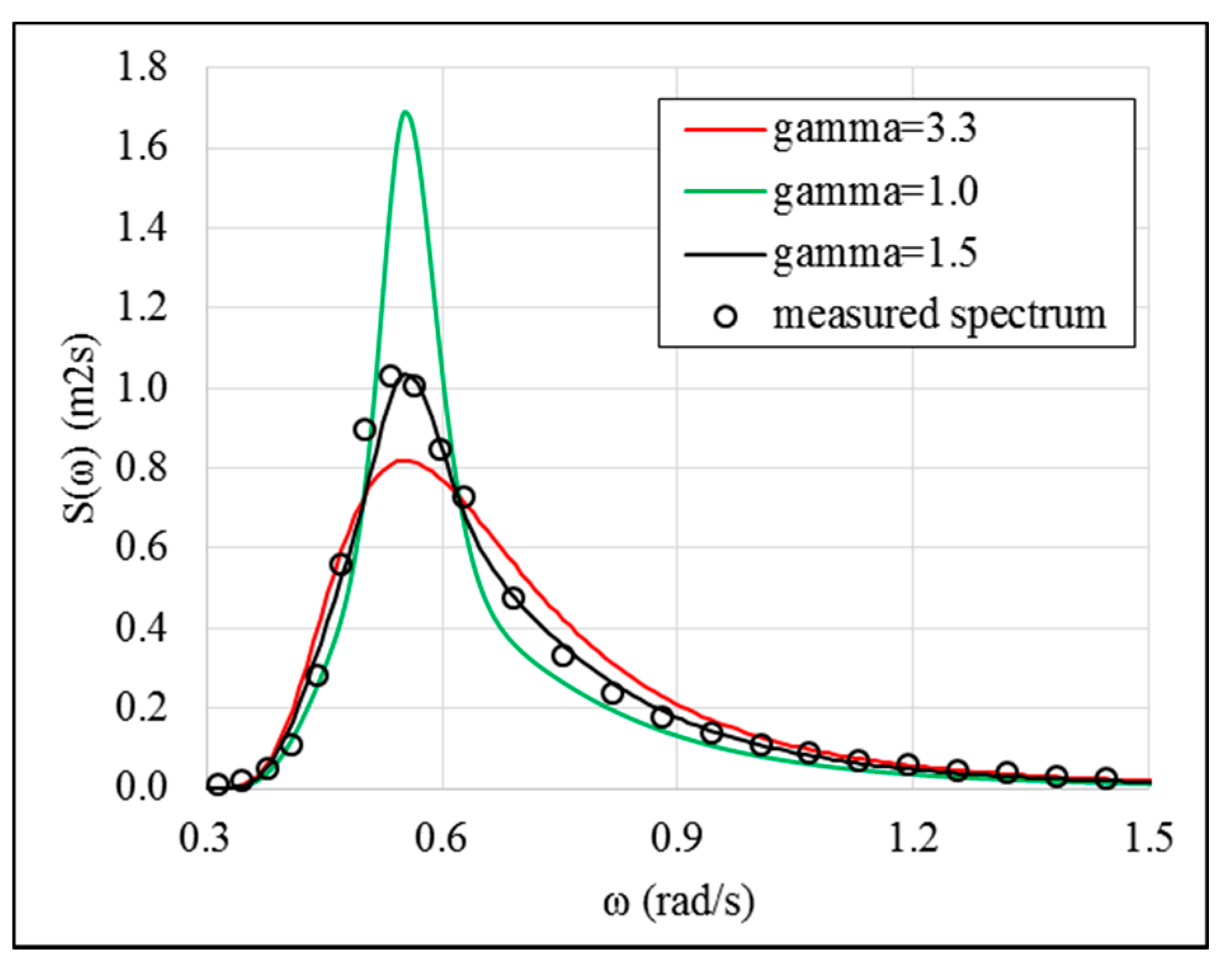
Figure 12.
Comparison of the calculated wave power and the corresponding error using different methods for measured waves at AMETS (water depth = 50 m). (a) Calculated wave power; (b) Error.
Figure 12.
Comparison of the calculated wave power and the corresponding error using different methods for measured waves at AMETS (water depth = 50 m). (a) Calculated wave power; (b) Error.


Table 1.
Wave power assessment for AMETS (bin size: 0.5 m & 0.5 s).
| Water Depth (m) | Method | Individual Spectra (I) | Average Spectra (II) | Error1 (%) between (I) and (II) | ||
|---|---|---|---|---|---|---|
| Pirr (kW/m) | Error0 (%) | Pirr (kW/m) | Error0 (%) | |||
| 50 | Accurate | 37.59 | - | 37.59 | - | 0.00 |
| DeepWater | 33.80 | −10.08 | 33.80 | −10.08 | 0.00 | |
| zero-order with ωe | 37.09 | −1.33 | 37.09 | −1.33 | 0.00 | |
| zero-order with ωp | 38.99 | 3.72 | 39.04 | 3.86 | 0.13 | |
| 3rd-order | 36.68 | −2.42 | 36.68 | −2.42 | 0.00 | |
| 4th-order | 38.48 | 2.37 | 38.48 | 2.37 | 0.00 | |
| 5th-order | 37.34 | −0.67 | 37.33 | −0.69 | −0.03 | |
| 25 | Accurate | 37.97 | - | 37.97 | - | 0.00 |
| DeepWater | 33.80 | −10.98 | 33.80 | −10.98 | 0.00 | |
| zero-order with ωe | 39.53 | 4.11 | 39.54 | 4.13 | 0.03 | |
| zero-order with ωp | 38.45 | 1.26 | 38.51 | 1.42 | 0.16 | |
| 3rd-order | 36.17 | −4.74 | 36.17 | −4.74 | 0.00 | |
| 4th-order | 38.68 | 1.87 | 38.68 | 1.87 | 0.00 | |
| 5th-order | 38.33 | 0.95 | 38.33 | 0.95 | 0.00 | |
Note: ‘Error0’ is the error compared to the accurate wave energy, and ‘Error1’ is the error compared each other for same approximation method (same convention will be used below).
Table 2.
Wave power assessment for AMETS (water depth: 50 m).
| Method | Bin Size: 1.0 m & 1.0 s | Bin Size: 2.0 m & 2.0 s | ||
|---|---|---|---|---|
| Pirr (kW/m) | Error1 (%) | Pirr (kW/m) | Error1 (%) | |
| Accurate | 37.59 | 0.00 | 37.59 | 0.00 |
| DeepWater | 33.80 | 0.00 | 33.57 | −0.68 |
| zero-order with ωe | 37.08 | −0.03 | 36.78 | −0.84 |
| zero-order with ωp | 39.06 | 0.18 | 38.87 | −0.31 |
| 3rd-order | 36.69 | 0.03 | 36.45 | −0.63 |
| 4th-order | 38.48 | 0.00 | 38.2 | −0.73 |
| 5th-order | 37.33 | −0.03 | 37.05 | −0.78 |
Table 3.
Wave power assessment for AMETS (bin size: 0.5 m & 0.5 s).
| Water Depth (m) | Method | Individual Spectra (I) | Scatter Diagram (II) | Error1 (%) between (I) and (II) | ||
|---|---|---|---|---|---|---|
| Pirr (kW/m) | Error0 (%) | Pirr (kW/m) | Error0 (%) | |||
| 50 | Accurate | 37.59 | - | 37.59 | - | - |
| DeepWater | 33.8 | −10.08 | 34.08 | −9.34 | 0.21 | |
| zero-order with ωe | 37.09 | −1.33 | 37.4 | −0.51 | 0.49 | |
| zero-order with ωp | 38.99 | 3.72 | 38.96 | 3.64 | 0.03 | |
| 3rd-order | 36.68 | −2.42 | 36.96 | −1.68 | 0.16 | |
| 4th-order | 38.48 | 2.37 | 38.87 | 3.41 | 0.16 | |
| 5th-order | 37.34 | −0.67 | 37.41 | −0.48 | −0.03 | |
| 25 | Accurate | 37.97 | - | 37.97 | - | - |
| DeepWater | 33.8 | −10.98 | 34.08 | −10.24 | 0.21 | |
| zero-order with ωe | 39.53 | 4.11 | 39.84 | 4.92 | 0.18 | |
| zero-order with ωp | 38.45 | 1.26 | 38.62 | 1.71 | 0.16 | |
| 3rd-order | 36.17 | −4.74 | 36.5 | −3.87 | 0.19 | |
| 4th-order | 38.68 | 1.87 | 39.34 | 3.61 | 0.36 | |
| 5th-order | 38.33 | 0.95 | 38.57 | 1.58 | −0.03 | |
Table 4.
Wave power assessment for AMETS (water depth: 50 m).
| Method | Bin Size: 0.5 m and 1.0 s | Bin Size: 1.0 m and 1.0 s | Bin size: 2.0 m and 2.0 s | |||
|---|---|---|---|---|---|---|
| Pirr (kW/m) | Error1 (%) | Pirr (kW/m) | Error1 (%) | Pirr (kW/m) | Error1 (%) | |
| Accurate | 37.59 | 0.00 | 37.59 | 0.00 | 37.59 | 0.00 |
| DeepWater | 33.87 | 0.21 | 34.08 | 0.83 | 34.29 | 1.45 |
| zero-order with ωe | 37.17 | 0.22 | 37.4 | 0.84 | 37.65 | 1.51 |
| zero-order with ωp | 39.03 | 0.10 | 38.96 | −0.08 | 36.87 | −5.44 |
| 3rd-order | 36.72 | 0.11 | 36.96 | 0.76 | 37.2 | 1.42 |
| 4th-order | 38.5 | 0.05 | 38.87 | 1.01 | 39.56 | 2.81 |
| 5th-order | 37.32 | −0.05 | 37.41 | 0.19 | 37.57 | 0.62 |
© 2017 by the authors. Licensee MDPI, Basel, Switzerland. This article is an open access article distributed under the terms and conditions of the Creative Commons Attribution (CC BY) license (http://creativecommons.org/licenses/by/4.0/).
Share and Cite
MDPI and ACS Style
Sheng, W.; Li, H.; Murphy, J. An Improved Method for Energy and Resource Assessment of Waves in Finite Water Depths. Energies 2017, 10, 1188. https://doi.org/10.3390/en10081188
AMA Style
Sheng W, Li H, Murphy J. An Improved Method for Energy and Resource Assessment of Waves in Finite Water Depths. Energies. 2017; 10(8):1188. https://doi.org/10.3390/en10081188
Chicago/Turabian StyleSheng, Wanan, Hui Li, and Jimmy Murphy. 2017. "An Improved Method for Energy and Resource Assessment of Waves in Finite Water Depths" Energies 10, no. 8: 1188. https://doi.org/10.3390/en10081188
Note that from the first issue of 2016, this journal uses article numbers instead of page numbers. See further details here.