The UK Solar Farm Fleet: A Challenge for the National Grid? † †


Centre for Renewable Energy Systems Technology (CREST), Wolfson School of Mechanical, Electrical and Manufacturing Engineering, Loughborough University, Loughborough LE11 3TU, UK
*
Author to whom correspondence should be addressed.
†
This paper is an extension of work originally reported in “Palmer, D.; Koubli, E.; Betts, T.R.; Gottschalg, R. Space and time analysis of irradiation variation across the UK: A 10 year study of solar farm yield. In Proceedings of the 12th Photovoltaic Science, Applications and Technology Conference, Liverpool, UK, 6–8 April 2016”.
Energies 2017, 10(8), 1220; https://doi.org/10.3390/en10081220
Submission received: 3 May 2017
/
Revised: 9 August 2017
/
Accepted: 14 August 2017
/
Published: 17 August 2017
Abstract
:Currently, in the UK, it is widely believed that supply from renewable energy sources is capable of reaching proportions too great for the transmission system. This research investigates this topic objectively by offering an understanding of year-to-year and area-to-area variability of PV (photovoltaic) performance, measured in terms of specific yield (kWh/kWp). The dataset is created using publicly available data that gives an indication of impact on the grid. The daily and seasonal variance is determined, demonstrating a surprisingly good energy yield in April (second only to August). The geographic divergence of generation from large scale solar systems is studied for various sized regions. Generation is compared to demand. Timing of output is analyzed and probability of achieving peak output ascertained. Output and demand are not well matched, as regards location. Nevertheless, the existing grid infrastructure is shown to have sufficient capacity to handle electricity flow from large scale PV. Full nameplate capacity is never reached by the examples studied. Although little information is available about oversizing of array-to-inverter ratios, this is considered unlikely to be a major contributor to grid instability. It is determined that output from UK solar farms currently presents scant danger to grid stability.
1. Introduction
The quantity of grid-connected large-scale PV (photovoltaic) systems has increased over the last few years and has also become more spatially distributed, both in the UK and worldwide. UK government policy in the form of the strategy of the UK Department for Business, Energy and Industrial Strategy (BEIS) towards solar PV appears supportive. The BEIS Solar PV Roadmap [1] states that solar projects should make a cost-effective contribution to carbon reduction, together with other forms of generation. Furthermore, solar installations should be deployed with regard to grid balancing and connectivity. Technical and economic challenges facing distribution systems are anticipated and indeed have been seen in countries such as Germany where a higher percentage of electricity is generated by PV [2]. Potentially, there could be overloads on the UK National Grid. Similarly, in Australia, it has been found that power outages are more likely in rural areas [3]. These locations have land available for large PV installations but the existing networks were designed to support distribution to the population. Sparsely populated rural areas have less dense networks. There is the potential for similar problems to arise in the UK. One of the essential 132 kV power lines in the South West has reached its full capacity. (See Appendix A for map of all UK locations. All maps produced using ArcGIS (ArcGIS Desktop: Release 10.1, Environmental Systems Research Institute (ESRI), Redlands, CA, USA). That is, connected and committed capacity equal the maximum rating of the circuit. Therefore, a delay of 3–6 years has been imposed on all new generation as this is requiring new infrastructure at 11 kV or above [4]. The overarching questions of this paper are whether this is justified or if variability of generation will mitigate the capacity limits, and how much energy would be lost if systems would need to down regulate.
Little work has been presented on temporally and spatially resolved generation and its link to existing infrastructure. There is no firm information on the percentage of time that the full rated capacity of the solar farm fleet is attained. It is not sufficient to examine individual systems and then simply scale up to the installed capacity as there is a significant variance between the systems due to the distinct weather patterns of the UK. This misrepresents the situation. The UK is also somewhat different to other countries with larger PV contributions, such as Italy and Germany, as it is an island with limited interconnects to other electricity systems and the weather patterns are more localized. The UK currently has over 15 GWp of PV from solar farms [5]. Summer peak power demand is approximately 20 GW. Together with conventional generation, this gives the impression that at certain times of year excess supply will overload the grid.
This paper investigates spatial and temporal variability of the UK’s PV system fleet. Hour-by-hour production of every large-scale solar installation in the UK is simulated. The generation of each solar farm is compared to the power-carrying capacity of adjacent high voltage lines, as well as to local demand. Spatial and temporal variability of PV generation in the UK are demonstrated. Two sets of analyses are performed on areas of different sizes. Firstly, PV generation is studied by aggregation to distribution network operator (DNO) area because these organizations are responsible for operational security. Furthermore, few local network power lines cross DNO boundaries. Subsequently, each PV installation is allocated to its nearest grid supply point (GSP). There is an average of 20 GSPs per DNO. GSP areas are thus much smaller than DNO areas. Grid supply points are used in the national demand forecast. Supply points with the highest input are identified and accessibility of PV systems to the grid are determined.
In addition, methods of assessing impact of solar farms on the grid are investigated. Potential overload may be viewed in terms of: a high number of solar farms in a given area; high total capacity of solar farms in a given area; distance of solar farm to the nearest grid connection point; and imbalance of supply and demand.
The effect of PV generation on each area of the grid (DNO or GSP) is estimated by calculating combined output based on solar farm installation data released by the Department of Climate Change Renewable Energy Planning database, REPD 2015 (575 × 1–50 MW installations at September 2015) [5]. (There are no details of electrical yield in the database, only information on the location and capacity of solar farms). It is assumed that all these PV systems are south-facing with an elevation of 22 degrees and comprise crystalline silicon module types. A bespoke simulation is based around these standardized system configurations. DC and AC energy output is calculated in all cases.
2. Calculation of PV Output Data
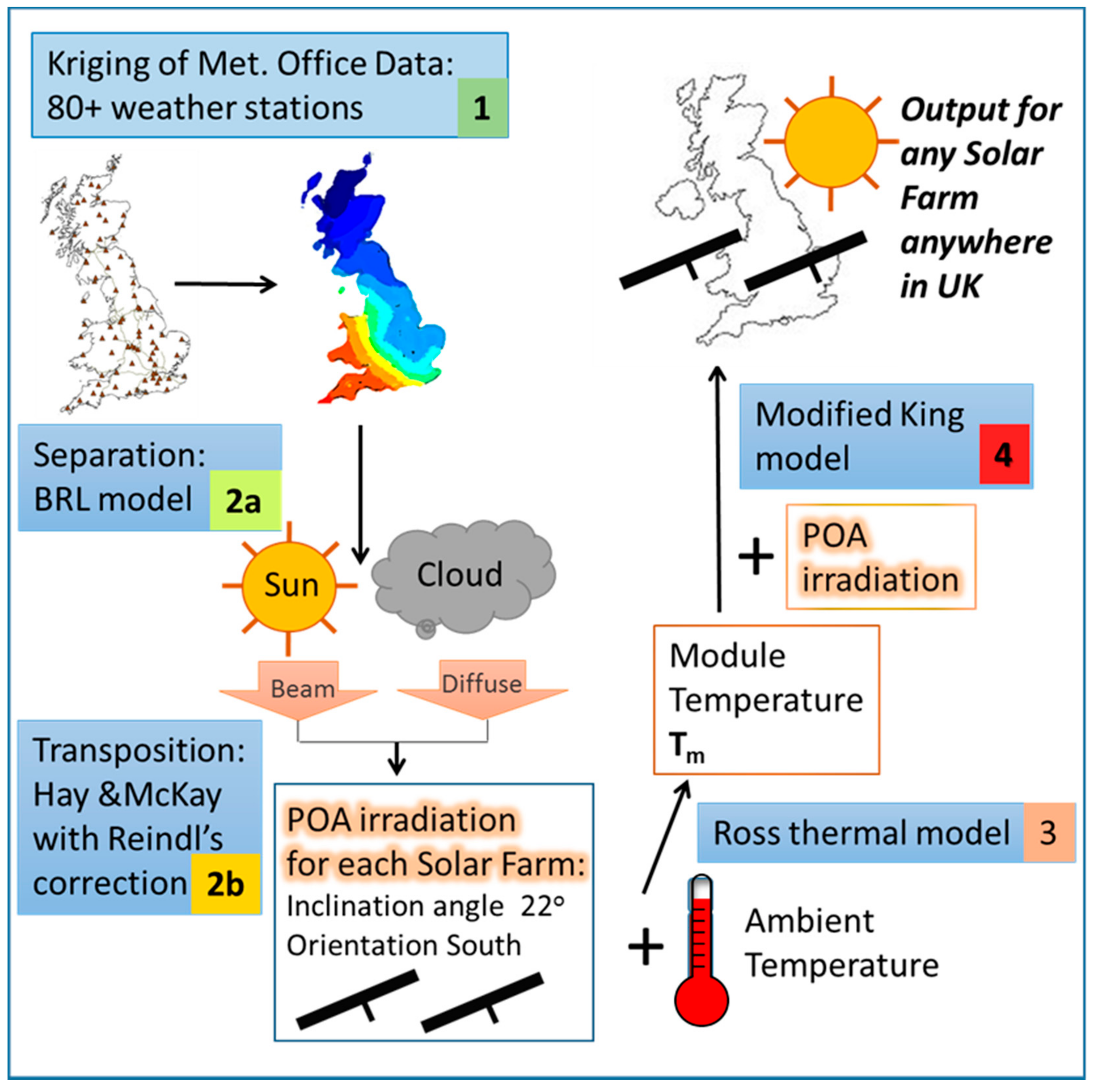
The PV output of each solar farm in the REPD 2015 was calculated in the stages described below and summarized in Figure 1, detailed validation and reasoning for the use of sub-models is to be presented elsewhere.
Stage one: data obtained from the UK Met. Office are interpolated. Input data is hourly global horizontal irradiation [6] and ambient temperature. The kriging method was selected following a review of interpolation techniques [7]. Kriging has performed well in many different areas of research [8]. This process delivers a seamless countrywide grid of local environments. The accuracy of this approach has been validated against a number of irradiance products, outperforming the best satellite models in places (details of the model as well as the validation are to be reported elsewhere in the near future [9]). Ten years’ data (2005–2014) was used as input to avoid annual biasing. There are over 80 unevenly distributed weather stations recording irradiation across the UK. Temperature data is more widely measured; almost 500 weather stations are available. To simulate the performance of existing PV systems, the environment at the grid point nearest each solar farm was selected as representing the actual location.
Stage two: the global horizontal irradiance values obtained for each solar farm are translated to in-plane irradiance. Firstly, beam and diffuse components are separated using a multivariate universal split algorithm [10]. This was found to deliver a lower root mean squared error compared to alternative univariate piecewise models for test sites dispersed across the UK. Secondly, the beam and diffuse components are individually transposed to the inclined plane [11,12].
Stage three: the in-plane irradiance obtained in stage two and ambient temperature from stage one are used to calculate module temperature using a thermal model [13].
Stage four: finally, an electrical model is employed to compute output power, taking plane-of-array (POA) irradiation and module temperature as inputs. Its basis is a simplified King’s model [14] for the maximum power point with adjusted coefficients. More details of the applied thermal and electrical models are given in [15].
3. Method Development for Aggregation of Data
3.1. PV Analysis by DNO Area
DNO areas were derived from Lower Super Output Area (LSOA) boundaries downloaded from the Office of National Statistics website. A lookup table from Elexon (entity responsible for delivering the “Balancing and Settlement Code (BSC)”, i.e., the operation of the UK’s electricity trading arrangements) was used to dissolve internal boundaries and create the larger DNO regions.
Aggregating to DNO level proved to be more involved than anticipated. Taking the average irradiance of all solar farms falling within the area and the total output (Solar Farm Average technique in Table 1) resulted in idiosyncratic descriptors. For instance, Yorkshire (northeast area of UK; generally speaking a lower irradiance area than the South of the UK) appeared to have the highest annual global horizontal irradiation (GHI) of all the DNOs. This problem sometimes occurs when a point-based map is aggregated to an areal unit. The interpretation of the data the map depicts (GHI) depends on the size and shape of the boundaries (e.g., DNO areas, GSP areas, LSOA etc.) imposed on the map. Known as the Modifiable Area Unit problem (MAUP), this was recognized over 70 years ago, but is still discounted by many analysts as insoluble [16]. Nevertheless, proposed solutions include:
- Use of individual (non-aggregated) data points (solar farms).
- Kernel density surface (a grid is created and density of points (solar farms) is calculated using a circle of a given radius centered on each grid cell and then moves on).
- Optimal zoning, i.e., derive areas scientifically by equal allocation of solar farms or based around solar farm clusters.
These approaches are independent of arbitrary administrative boundaries. However, none of them are familiar to PV consultants or energy analysts, so an alternative was sought. The techniques summarized in Table 1 were tested.
The results of experimenting with these techniques for the Southwest DNO are given in Table 2. The calculated average hourly GHI for 2014 produced for the entire Southwest DNO using each of the techniques is compared to the calculated average hourly GHI for the solar farm furthest from the DNO centroid. (The Southwest DNO has 175 Farms and the furthest from the centroid is 134 km away). The purpose is to ascertain which technique minimizes differences.
Table 2 gives five different possible values for DNO irradiance. The difficulty is to choose the value most representative of the DNO as a whole. It can be seen that there is very little difference between Centre Point and DNO average numbers. The DNO average technique cannot provide accurate input to the beam/diffuse separation model, therefore the Centre Point technique was chosen. All techniques have supporting and opposing arguments. The Centre Point technique is chosen as follows because it minimizes differences for outlying solar farms.
The Centre Point technique may be summarized and clarified as follows:
- Global horizontal irradiation and ambient temperature values are produced by taking the interpolated value of the center point of the DNO area. (As opposed to the first attempt, with the Solar Farm Average approach, when values nearest to the solar farm locations were selected and averaged/totaled);
- The latitude of the DNO centroid was used to calculate beam/diffuse separation and plane-of-array irradiance. Output was estimated using the electrical model and scaled-up by total capacity of solar farms in the area.
3.2. PV Analysis by GSP Area
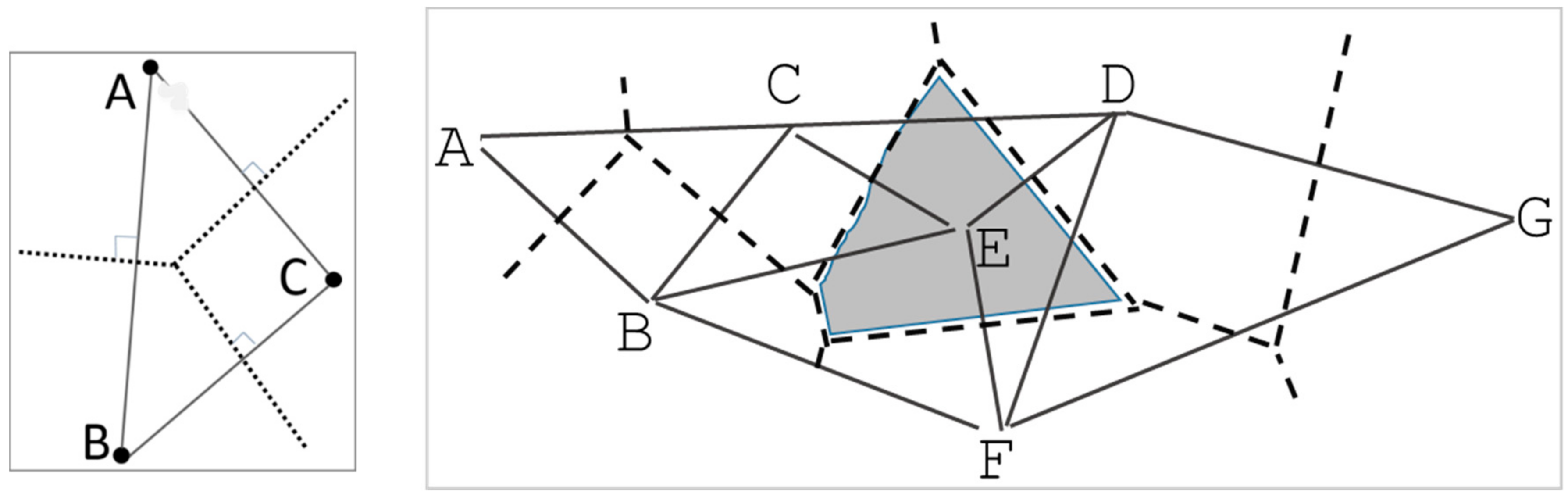
Grid supply points (400 kV) serving the transmission system were obtained National Grid map layers supplied by [17]. The electricity contribution areas of GSPs are not publicly available, so for each GSP, the area closest to it was selected as follows. Thiessen polygons were drawn as the supply areas of each GSP. These were constructed as listed below:
- Draw straight lines between the grid supply points (solid lines in Figure 2).
- Locate the mid-points of each of these lines and draw another line, at right angles to the solid line; these are shown as dashed lines in Figure 2.
- The dashed lines meet to form irregular polygons, as indicated by the shaded area in Figure 2. The solid lines are eventually deleted.
Thiessen polygons delineate zones of influence around each of a group of points. The boundary of each Thiessen polygon encloses the area that is closer to the point it surrounds than any other point [18]. This enables individual PV systems to be allocated to specific feeders.
4. Results and Discussion
The aim is to identify how much of a strain current installations already place on the network, and to deliver a methodology to assess the impact of further deployment. The assumption is that PV energy is not down-regulated and the remainder of the network is responsive. The current assumption is that all systems work synchronously, a view challenged below. The work below demonstrates that the overall time PV installations pose a risk is much smaller than currently being assumed and the impact on annual generation of individual systems of e.g., curtailment may be less than assuming synchronous operation. The assumption here is that curtailment is only necessary if all systems reach capacity, which is true for current installation levels. The underlying data will be made available with the possibility to assess additional installations to allow the simulation of future trends.
The key is an investigation of the spatial and temporal variability of PV generation in the UK. Different spatial resolutions (unaggregated, DNO area and GSP area) are used to demonstrate that it is not sensible to treat the entire system-ensemble as performing synchronously. Temporal resolutions are also considered. Finally, the number of times the UK solar farm fleet achieves full rated capacity is investigated to allow an investigation of the energy lost due required curtailment. It is shown that treating systems individually minimizes the frequency of full performance as weather fronts reduce the number of incidents where the system reaches capacity.
4.1. Spatial Generation Analysis
4.1.1. Individual Solar Farm Level Examination
The output of solar farms must reach consumers. Ideally, solar farms should be adjacent to, and temporally overlap with demand, but this is not the case in the UK.
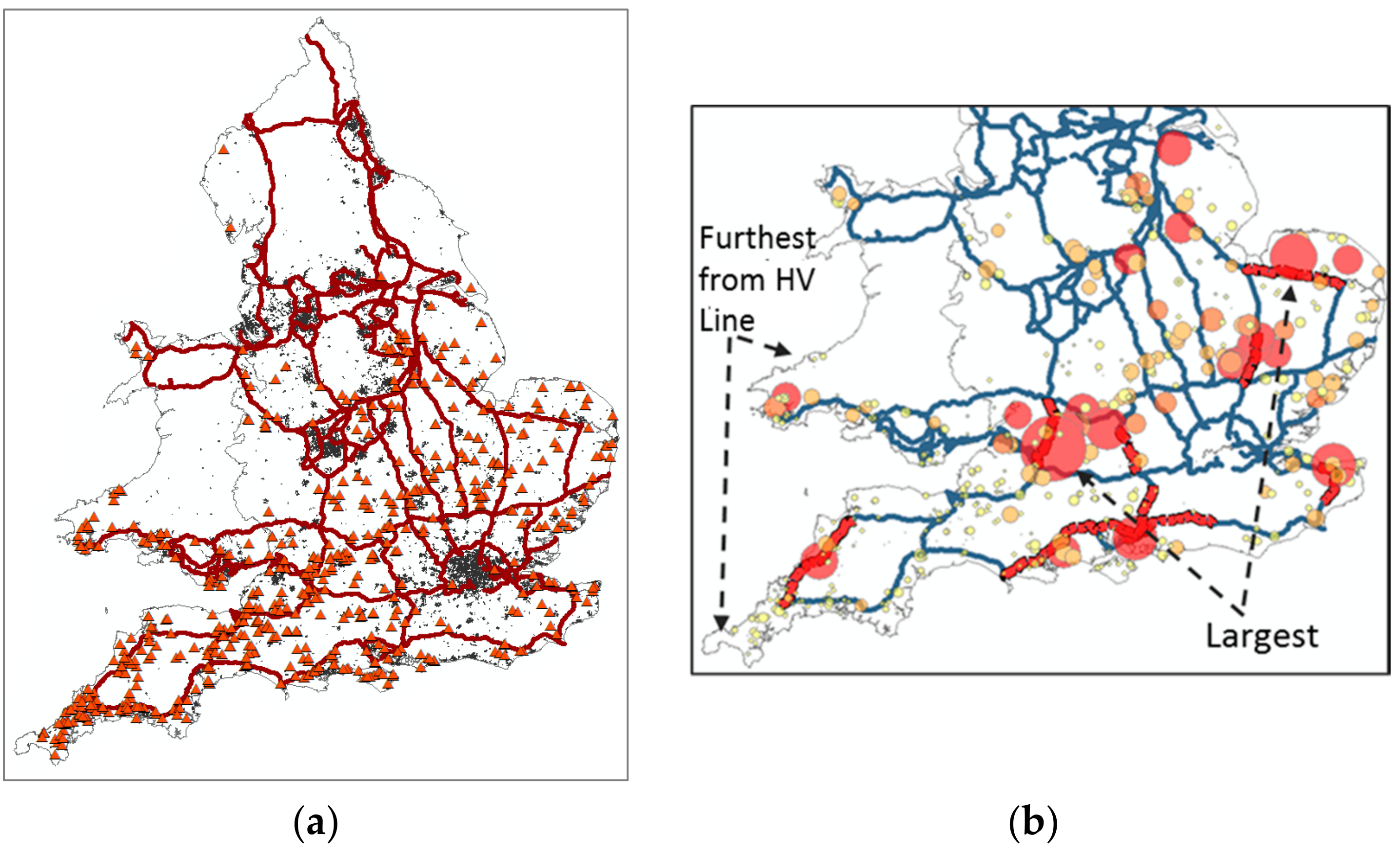
To assess the ability of the system to accept power, it is necessary to know the high voltage power line to which the system is connected. Figure 3a indicates that two-thirds of UK solar farms (orange triangles) are within 10 km of high voltage power lines (red lines). It is noticeable that solar farms in the UK are not in the proximity of centers of population (dark grey areas in Figure 3a) where demand is highest. The largest installations (larger and redder circles in Figure 3b) are over 100 km from London and other big cities, which means energy generated by these systems needs to be transported by the National Grid for significant distances and the ability of the high voltage power lines to transport this power becomes the limiting factor for further installations of PV.
Potential grid overload currently is considered such a risk in different localities, that certain areas will not accept further connections to the grid. However, this assessment is done on the basis that all systems will be operating at the same time to the same percentage. Below it will be shown that this is not the case, considering the worst affected power line. It will be shown below that this depends on how it is assessed. If high numbers of solar farms were indeed a problem as many regional electric companies perceive them to be, then the Southwest would already need to implement curtailments with consequent wastage of potential generation. Long transmission distances over local networks to the nearest high voltage line would again affect the extreme Southwest, as well as solar farms on the Welsh coast. This may introduce a phase shift in the power and power flow may be opposed to the design direction. High capacity of solar farms could cause surges in power lines close to the largest installations or generally high levels of injected power. Imbalance of supply and demand is also likely to affect the National Grid. This is investigated further in Section 4.1.3. In practice, the last two factors are probably the most relevant ones. This is because high capacity solar farms are capable of large and unanticipated power injections into the main grid. The high voltage lines which receive feeds from the ten highest capacity solar farms (i.e., highest power supplied to local substation) are marked as red broken lines in Figure 3b. They are nearly all located in rural or coastal regions, away from sources of demand.
4.1.2. DNO Area Examination
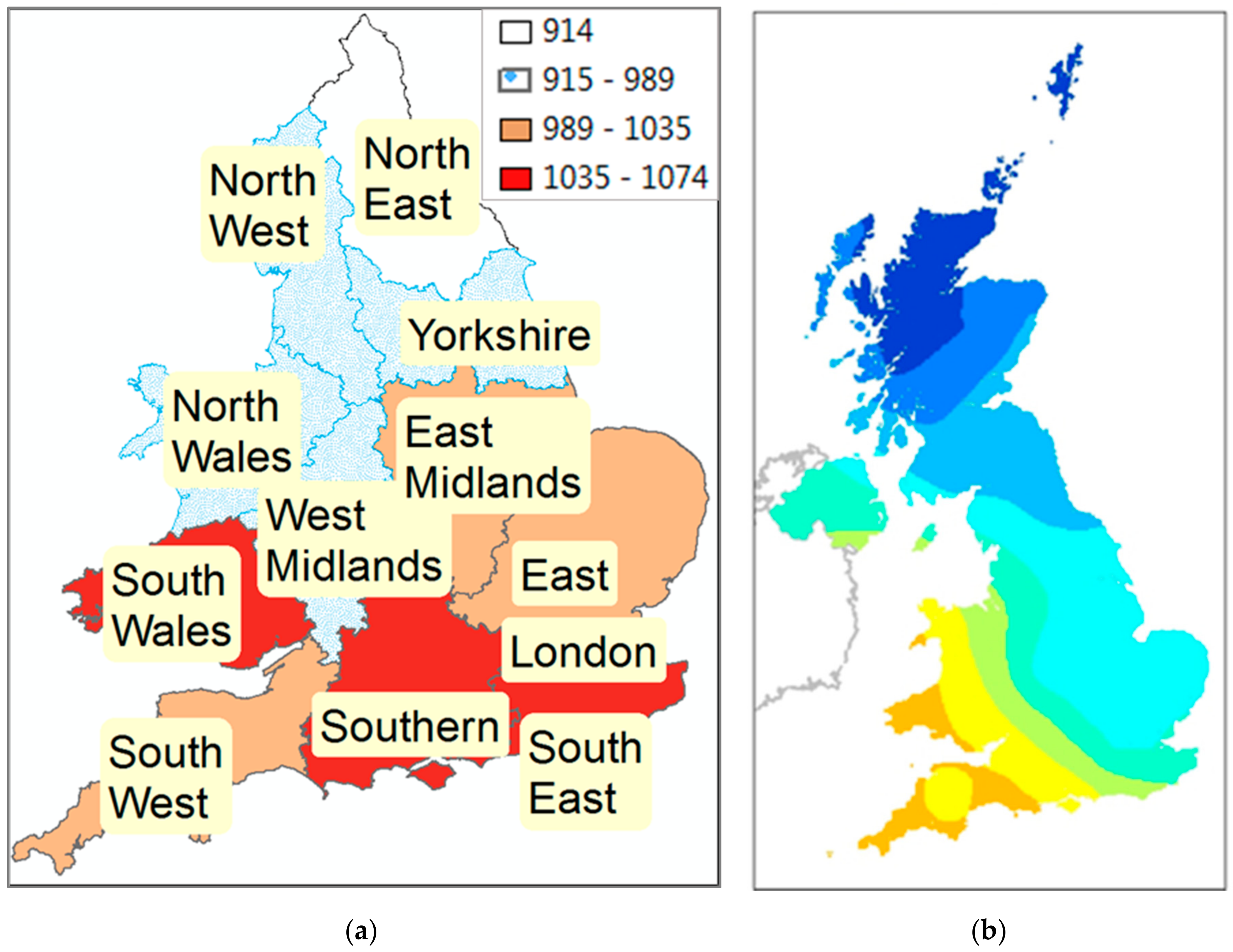
Initially, average annual global horizontal irradiation per DNO was used to investigate the presence of statistical bias due to aggregation. The results indicate the highest irradiation being observed in the south of the UK (Figure 4a), which is contrary to expectations as the Southwest is expected to have the highest. The highest non-aggregated irradiation is observed in the Southwest. This was investigated further and shown to be a feature of the integration areas. The DNO map in Figure 4a shows that the relatively large Southwest DNO area contains a circle of lower annual irradiation indicated in Figure 4b. This comprises the higher ground of Exmoor and Dartmoor national parks. Aggregating DNO levels are not the best choice for investigating variability of meteorological data, as just illustrated. Therefore, investigation is also carried out at the smaller GSP area level (Section 4.1.3).
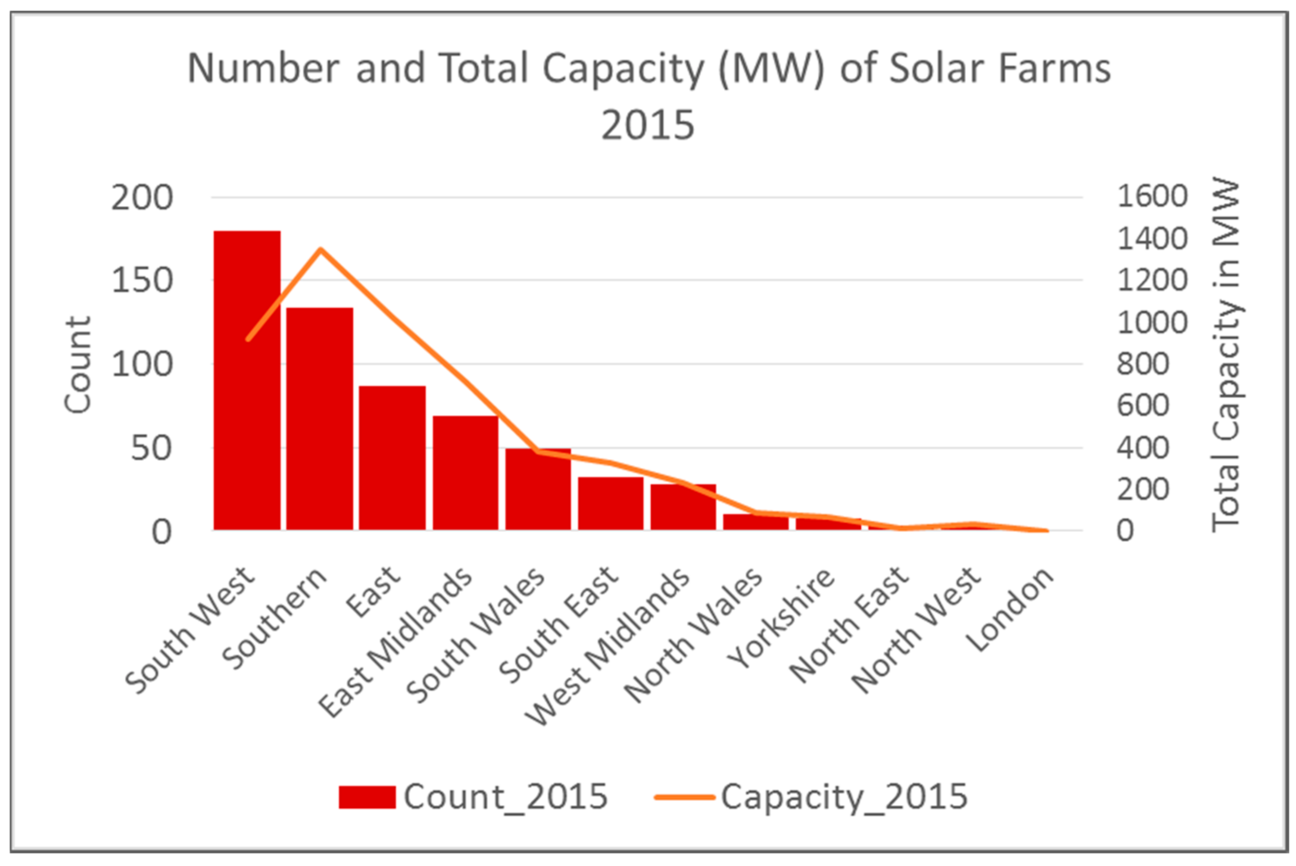
Siting of solar farms is somewhat influenced by the solar resource. Figure 5 shows that the highest number of large scale solar installations are currently found in the Southwest DNO. However, the Southern DNO had the largest installed nameplate capacity. This is because many moderately-sized solar farms are situated in the Southwest, whereas the South has fewer but larger installations. Field sizes are generally larger in the south.
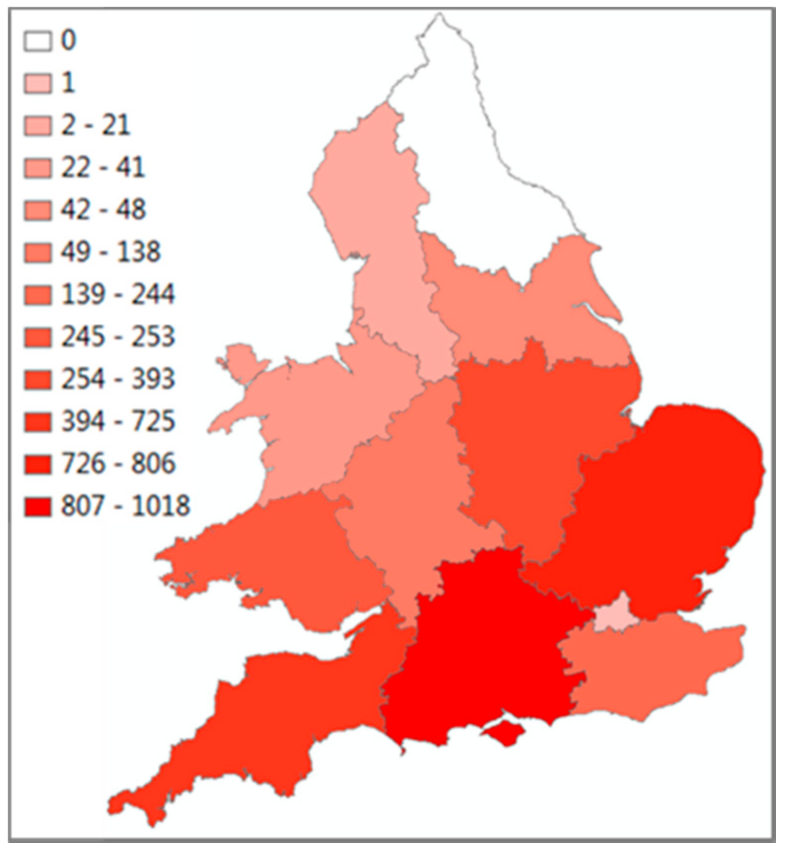
Figure 6 shows that the Southern DNO has the highest calculated output from solar farms due to possessing the highest installed capacity and highest solar resource at this level of aggregation.
4.1.3. GSP Area Examination
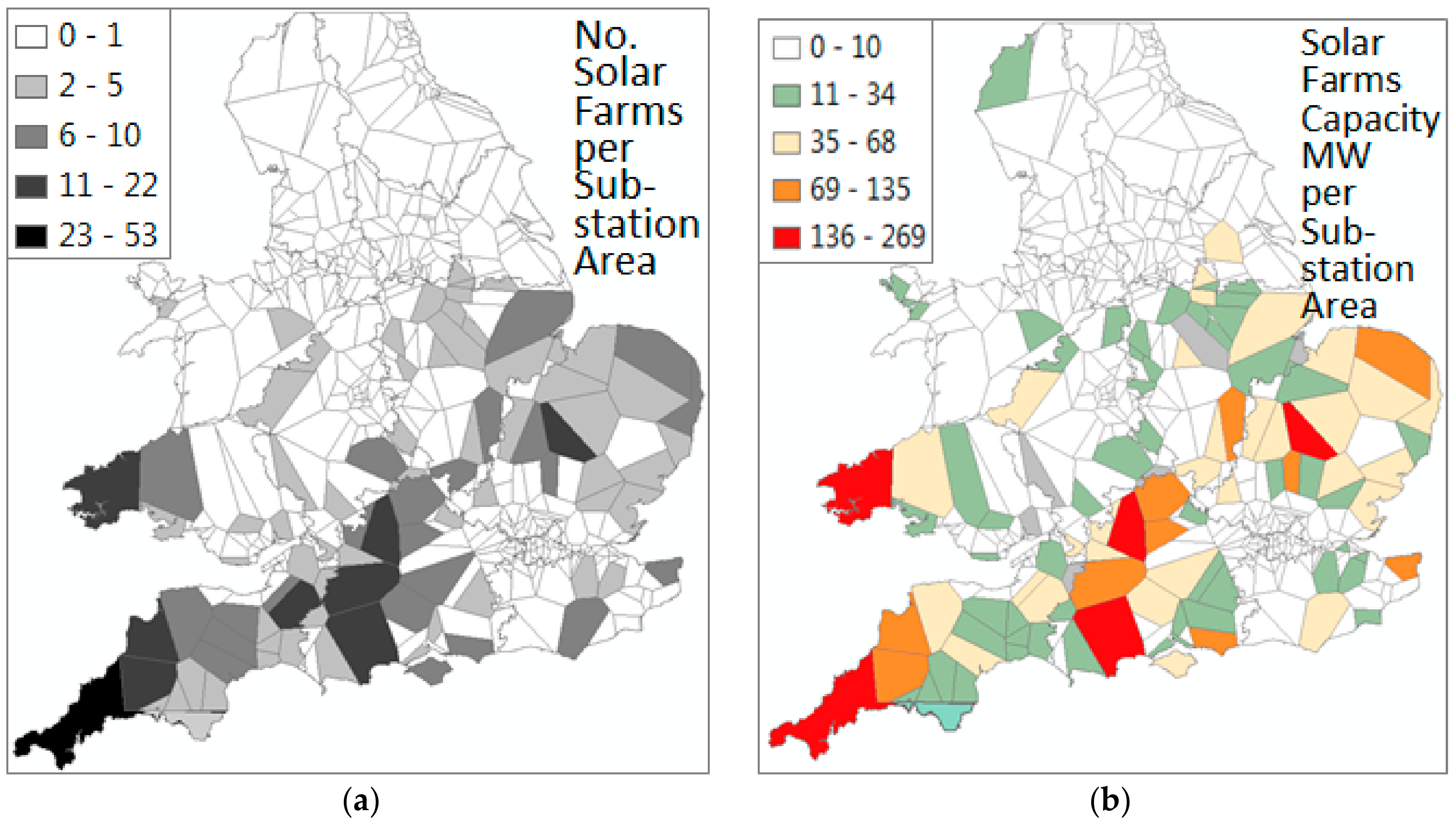
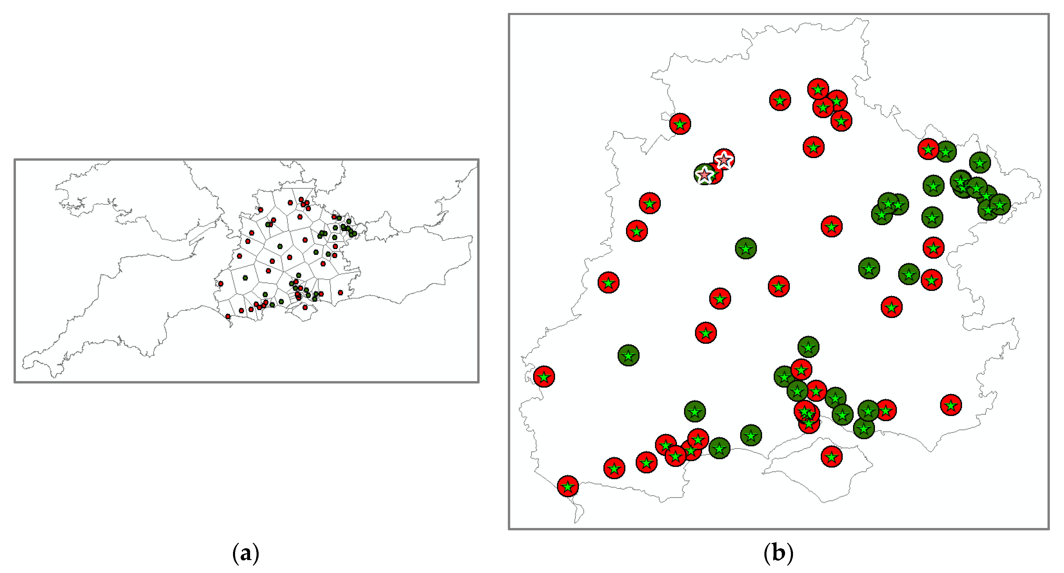
The high number of solar farms in the Southwest may also be observed at the GSP area level. It becomes obvious that they are concentrated at the extremity of the peninsular. The top number of PV installations feeding into the Indian Queens substation in Cornwall is visible in Figure 7a. However, in terms of input capacity, this substation is topped by Minety (in Wiltshire), Mannington (in Dorset), and Burwell near Cambridge (dark red areas on the right-hand side in Figure 7b).
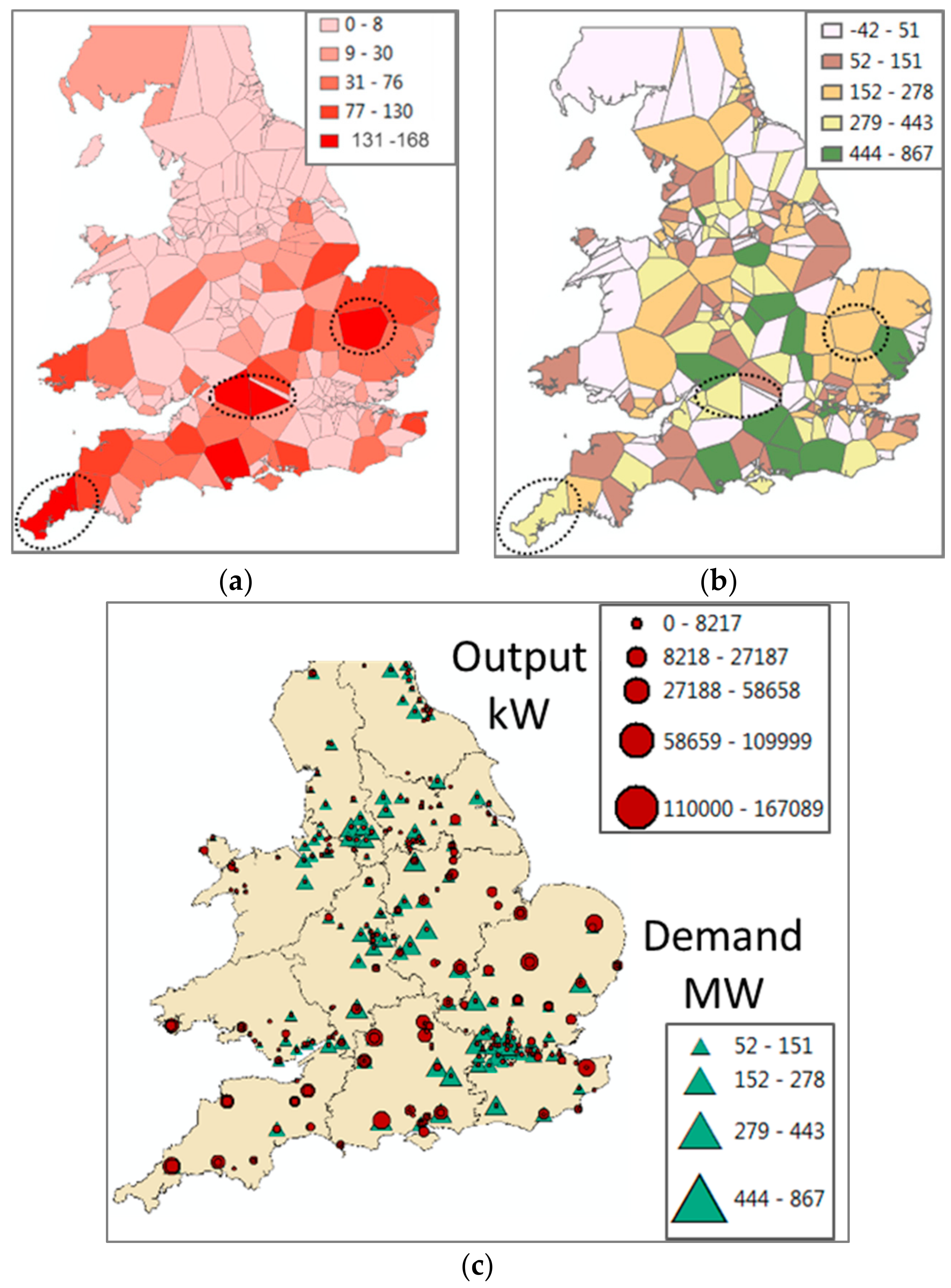
As mentioned previously, another form of grid limitation is the imbalance of supply and demand. Back-feeding can occur when generators on a particular feeder produce more energy than is consumed by the consumers at this particular connection point. High penetration can cause voltage control challenges for the grid operator. Figure 8 indicates that in the UK, electricity supply from solar farms and demand are mismatched geographically. Energy of solar farms is predominantly generated in rural areas and demand occurs predominantly in large cities, e.g., London (southeast) and Manchester (northwest). The GSP areas receiving the highest solar farm generation are circled in Figure 8a,b. They do not coincide with high demand areas. The demand may perhaps be seen more clearly in Figure 8c, where the grid supply points are represented as the original points and not the feed-in area of the point. The high demand GSPs (which serve small areas) in London are more visible as large triangles.
Figure 8a displays the expected high output in the Southwest. This is detectable at the GSP level of aggregation, but not at the DNO (Section 4.1.2). At the DNO level, consumption by far exceeds generation.
The analysis of generation and demand given above demonstrates significant spatial mismatch in demand and supply. This is enhanced by single feeders being more affected than others, as a significant percentage of the PV systems is located in the south and south-west, i.e., in areas with low demand and somewhat weak infrastructure (South-West).
4.1.4. Case Studies of Supply Points
From the analyses in Section 4.1.1, Section 4.1.2, Section 4.1.3, it appears that grid instability is a possibility in some parts of the UK. Fortunately, for a stable electricity grid, the situation is not so straightforward. Three case studies were analyzed. It was not practicable to manually retrieve the required information from network diagrams and photographs for all supply points on the National Grid, so these examples were selected to allow in-depth examination. These case studies have high numbers of solar farms which suggests inventions may become necessary to prevent outages. Closer examination of transformers, demand, and capacity finds this is not, in fact, required.
The UK National Grid comprises a number of voltage layers [20]. The lowest layer is the low voltage circuit (mains) which serves domestic consumers in private dwellings. The mains feed into secondary substations (11 kV feeder), which in turn feed into primary substations (33 kV feeder). The next layer is the 132 kV bulk supply points (BSP) and finally the highest voltage level (grid supply points (GSP), 400 or 275 kV). The number of substations decreases from the lowest to the highest layer. Here, the first case study examines a supply point in the GSP layer and the second analyses one in the BSP layer. The third case study moves up an order of magnitude to examine supply to a high voltage feeder.
Case Study One: Mannington Grid Supply Point
Mannington GSP is 1200 MW in size, i.e., 5 × 240 MW transformers. Based on Thiessen polygons (Section 3.2), the output from 22 solar farms passes through this GSP. The total capacity of these feed-in solar installations is 215 MW. Thus, even if all the solar farms achieve full capacity, and if the solar farm output is transmitted through one transformer (240 MW), overload will still not occur (these scenarios are highly unlikely—achievement of capacity is looked at in Section 4.3).
Case Study Two: Bulk Supply Points in Southern DNO
The Southern DNO has BSPs in 77 locations (as opposed to its 37 GSPs because they serve smaller areas). Information regarding the location, transformer size, demand, and constraints on the BSP imposed by the DNO Company was obtained from [21]. The total capacity of solar farms feeding into each BSP was calculated by assigning them to Thiessen polygons (Figure 9a). The minimum demand obtained from the DNO Company (Scottish and Southern Electricity Networks—SSEPD) was subtracted from total solar farm capacity to provide the net solar generation capacity. If the net capacity is greater than the transformer rating, the BSP is flagged as overloaded. The results are mapped in Figure 9b. BSPs identified as overloaded are marked by pink stars, those with adequate capacity by green. It may be seen that only two BSPs (upper left of map) are flagged as overloaded from solar generation. In reality, this is unlikely to hold true because these BSPs are close to the edge of the DNO region and some of the output allocated to them is probably distributed “over the border” into the neighboring DNO. So, in fact, solar generation poses minimal risk to the transmission network in this DNO area.
Figure 9b also shows constraints on connection to BSPs imposed by SSEPD. BSPs subject to DNO company constraints are represented by red circles, those without constraints by green. There are many more constraints than appear necessary from the solar output analysis. This is due to other forms of generation and network stresses. DNO companies also protect major food manufacturers and vital services e.g., hospitals.
The impact of solar farm output only on substations has been investigated here. Solar output in combination with nuclear and wind generation may cause circuits to exceed their limits. For instance, generator connections have been restricted in the Southwest until transmission system upgrades associated with the construction of the Hinckley Point C nuclear generator are complete [22].
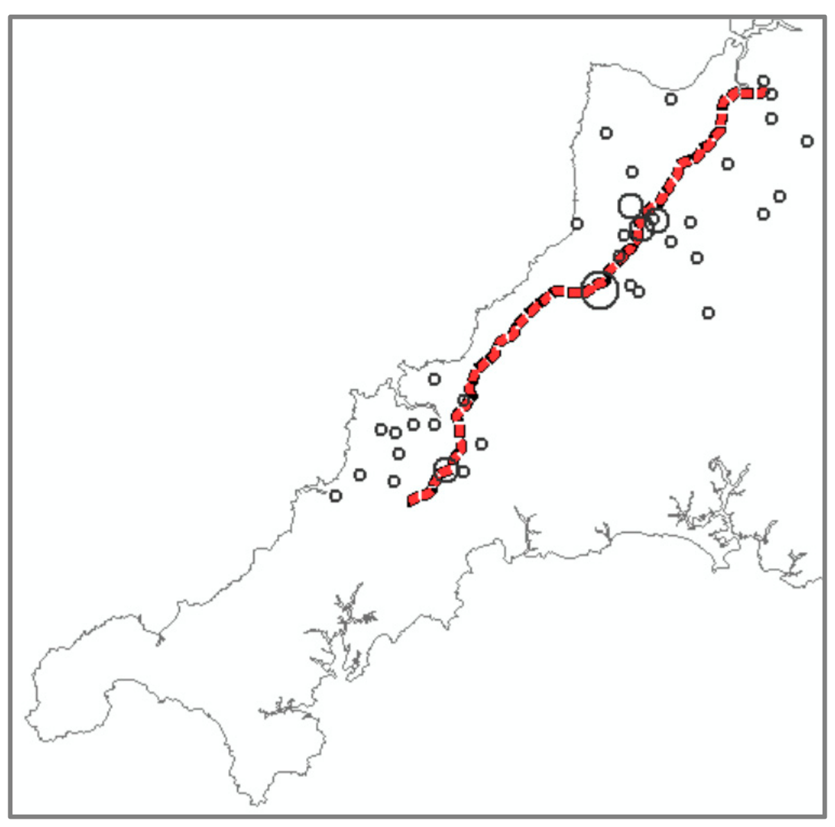
Case Study Three: Restricted Southwest Feeder
The restricted circuit referred to above is scrutinized in this section. The purely geographical aggregation is not sensible as it also depends strongly on the key feeders in the area. One of the worst impacted feeders in terms of PV penetration is investigated here. This particular feeder is seen to be “full” and further applications for connection will not be accepted subject prior to a major upgrade. The Route 4 VW—Alverdiscott—Indian Queens Taunton segment is surrounded by 37 solar farms, positioned 1.7 to 9.8 km from the high voltage line (Figure 10). Three-quarters of these solar farms have a capacity of 5 MW or less; seven range from 6 to 12 MW; and two may be described as large (18 and 40 MW). It may be seen that the large-scale installations are distributed along the length of the line. They do not cluster in one situation.
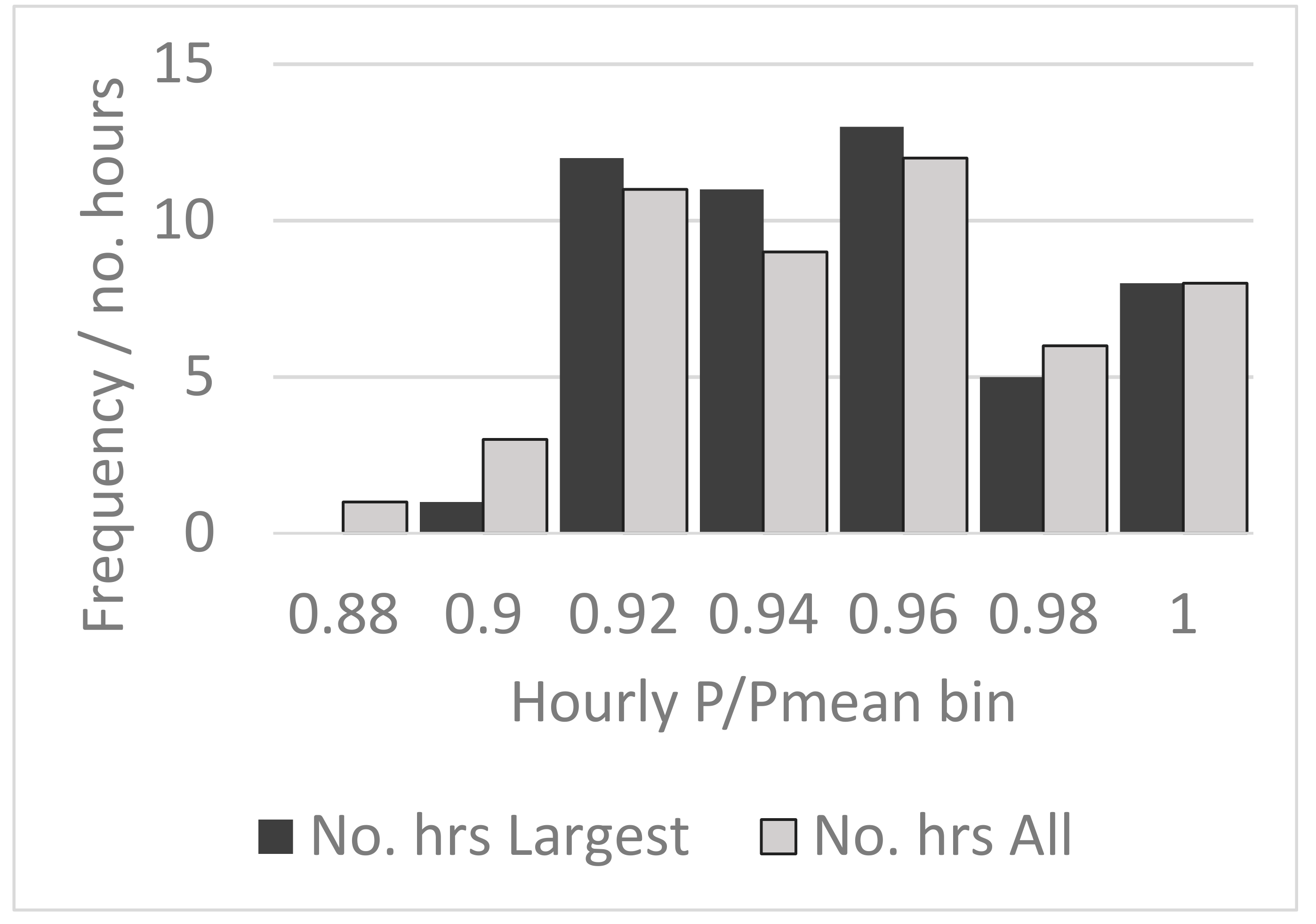
The largest (40 MW) solar farm achieved over 80% of nameplate capacity for 50 h of 2014 (part of the midday hours between April and July). Taking all 37 installations in aggregate, the ensemble did not achieve more than 60% capacity at any time during the year. Figure 11 contrasts the frequency of achievement of normalized power output of all 37 sites and the largest site for the 50 high capacity hours. It is evident that the ensemble approaches maximum capacity less frequently than the single large site. This smoothing is due to spread of site locations and the prevailing westerly weather system. This effect of smoothing due to environmental variability ameliorates potential overloading. The need for curtailment measures is reduced.
4.2. Temporal Resolution Analysis
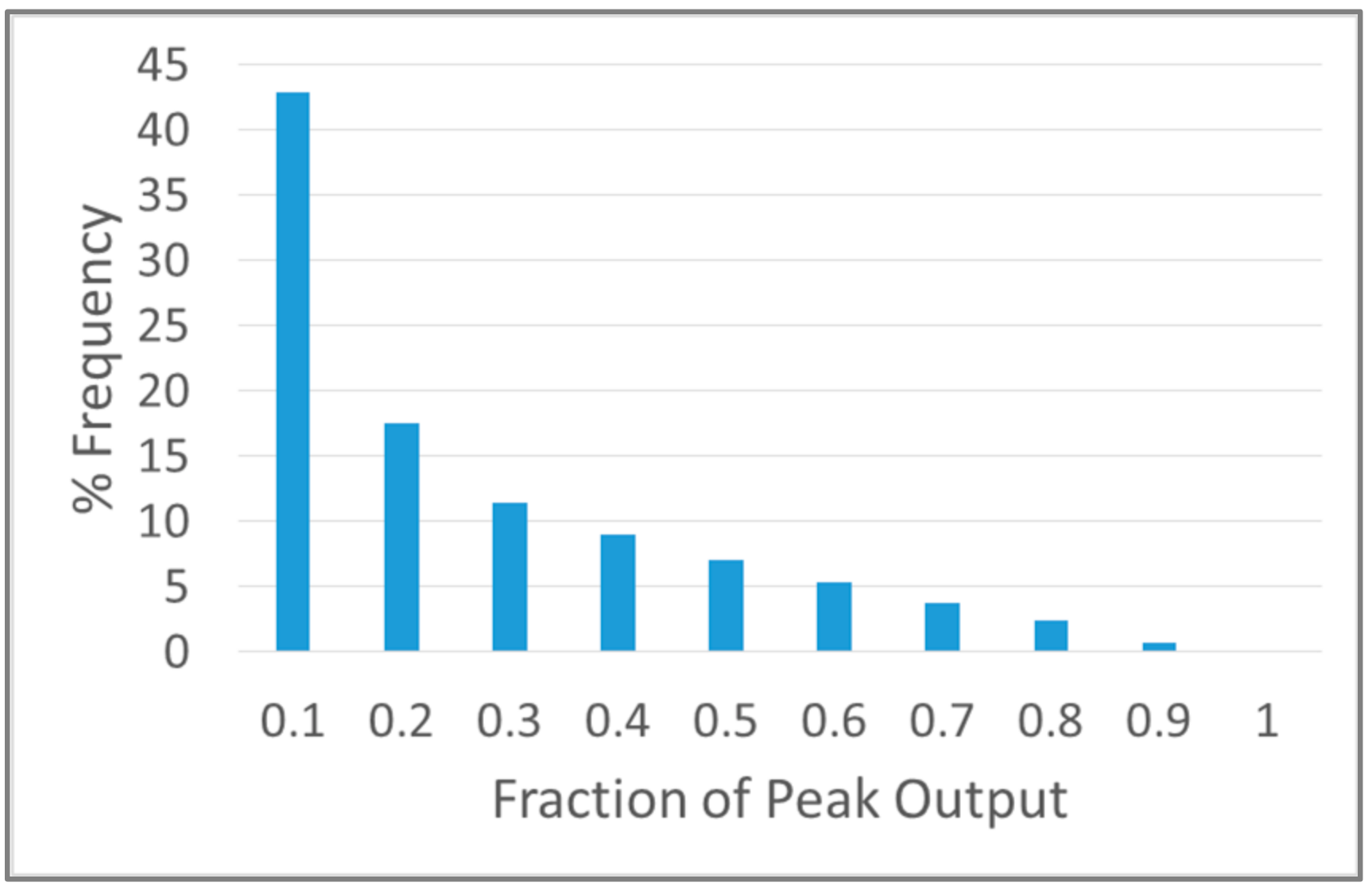
Average solar farm output per individual hour as a fraction of the peak power output is given in Figure 12 for ten years countrywide. This graph shows the percentage of daylight hours which achieve a given fraction of stated nameplate capacity. This is an independent measurement of the PV system performance in terms of energy generated divided by the nameplate Standard Test Conditions (STC) rating. Very low generation occurs for the vast majority of daylight hours. This is discussed further in Section 4.3 (the zero at 1 kWh/kWp is just the low number of hours). Individual DNOs show very similar patterns.
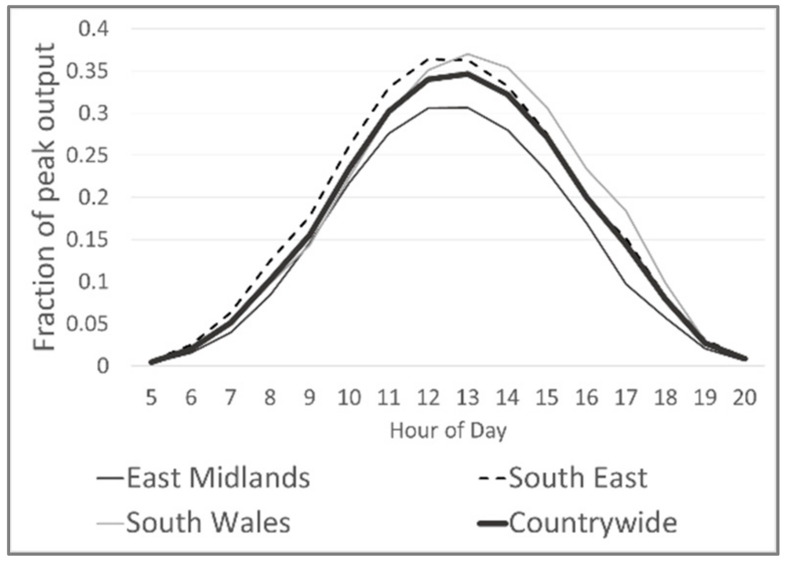
Hourly trends were analyzed for the UK as a whole and for individual DNOs (Figure 13 shows a sample for simplicity). The UK average value is highest at hour ending 1:00 pm. Those DNOs in the east of the country peak at noon, whilst westerly located DNOs peak slightly later, around 12:30 pm. This is purely due to Earth’s rotation but serves to smooth out injection somewhat. The DNO with the greatest kWh/kWp is South Wales. The lowest is the East Midlands (Figure 13). These tendencies are much as would be expected.
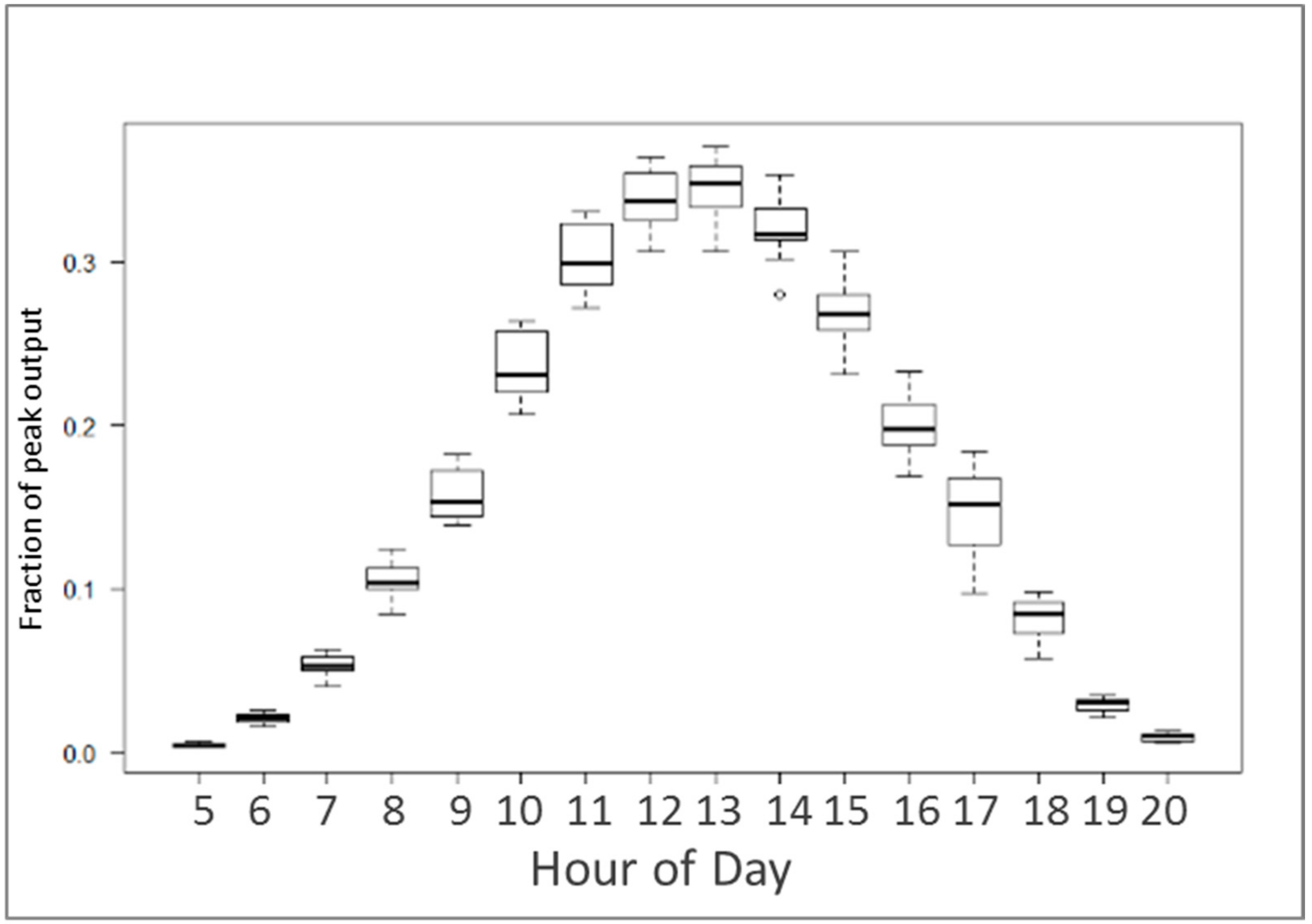
Variation of individual DNOs from the national average is demonstrated in Figure 14. The hours with the widest spread between areas are also the most productive hours, i.e., the middle of day. The difference in values may be explained by DNO latitude and longitude and the associated changing position of the sun.
Average hourly values are compared between years to establish inter-annual variation. The most variable hour for the whole country was found to be 2:00 pm. The hours with the largest standard deviation for single DNOs range from 11:00 am to 3:00 pm. This would indicate some smoothing potential as this is either weather or season related.
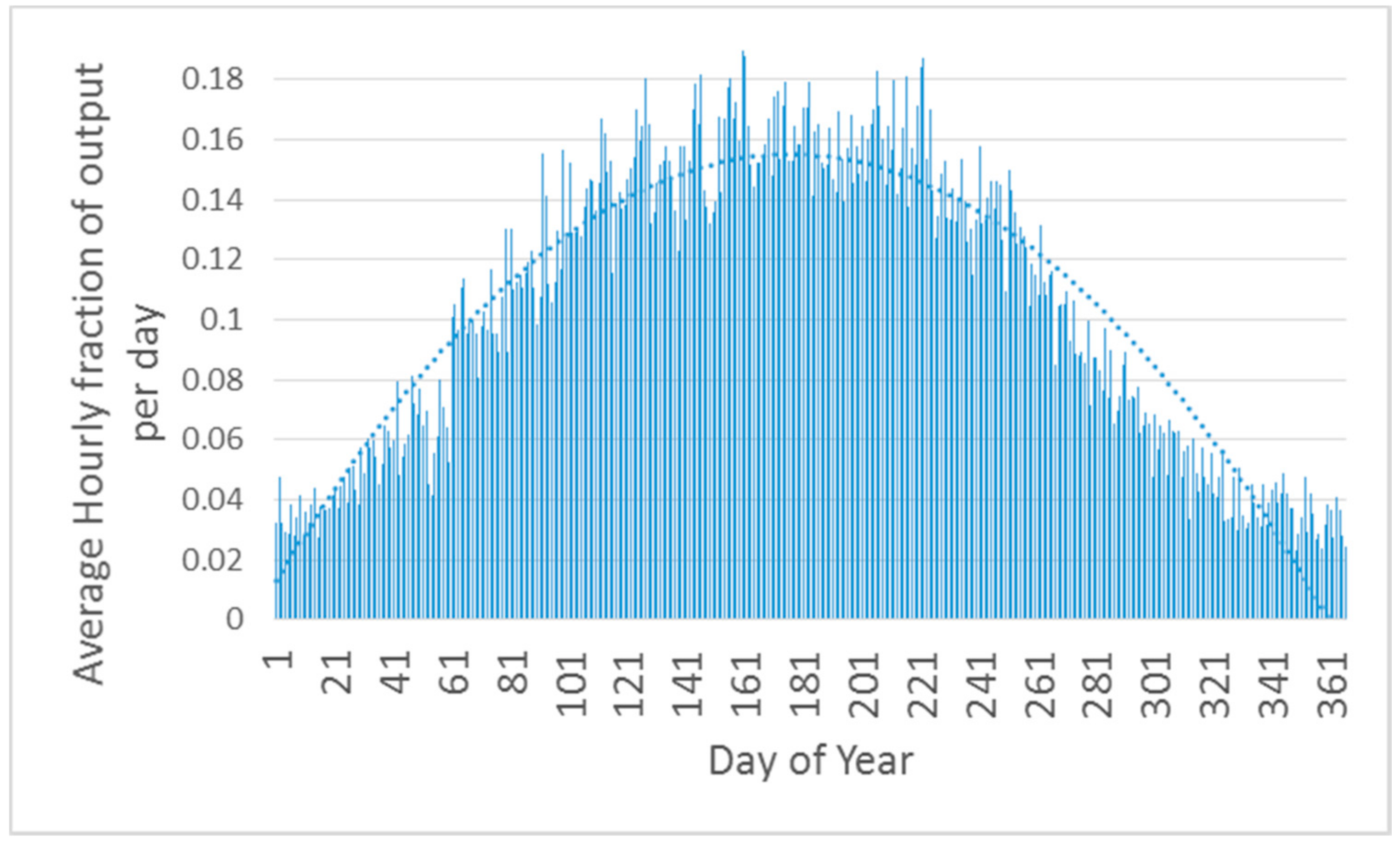
Moving to daily grouping of data reveals some interesting patterns (Figure 15). Daily higher and lower values than the prevailing tendency occur every 5–15 days. Figures are generally better than the overall trend from March to September and again during December when high pressure dominates the weather. Lower than expected values occur in blocks at the end of February (when the wind direction may veer north), late May (again the wind may be northerly) and from the end of September to the beginning of December (autumn storms).
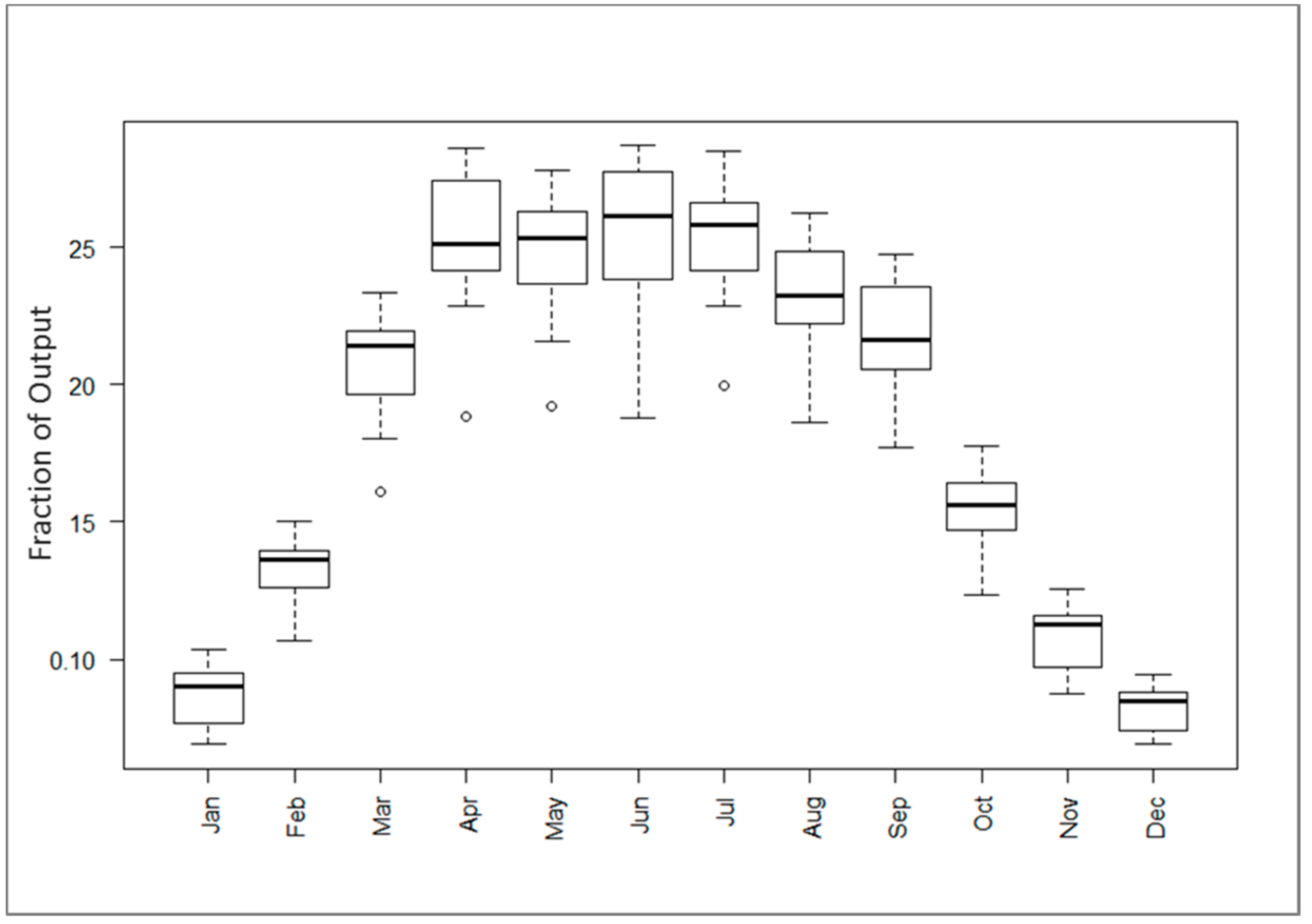
Monthly figures rise to June and then fall away (Figure 16). It may also be noted that June has the greatest variance between DNOs compared to the other months. This may be due to the different regional climates which occur in the UK. Differences are enhanced in summer when some regions are much drier than others. In addition, April has higher than expected values and is also the month with the greatest inter-annual variability. One possible explanation is that irradiance values begin to increase in the spring whilst temperatures can still be low, a combination that enhances PV output.
4.3. How Often is Full Capacity Achieved by the UK Solar Farm Fleet?
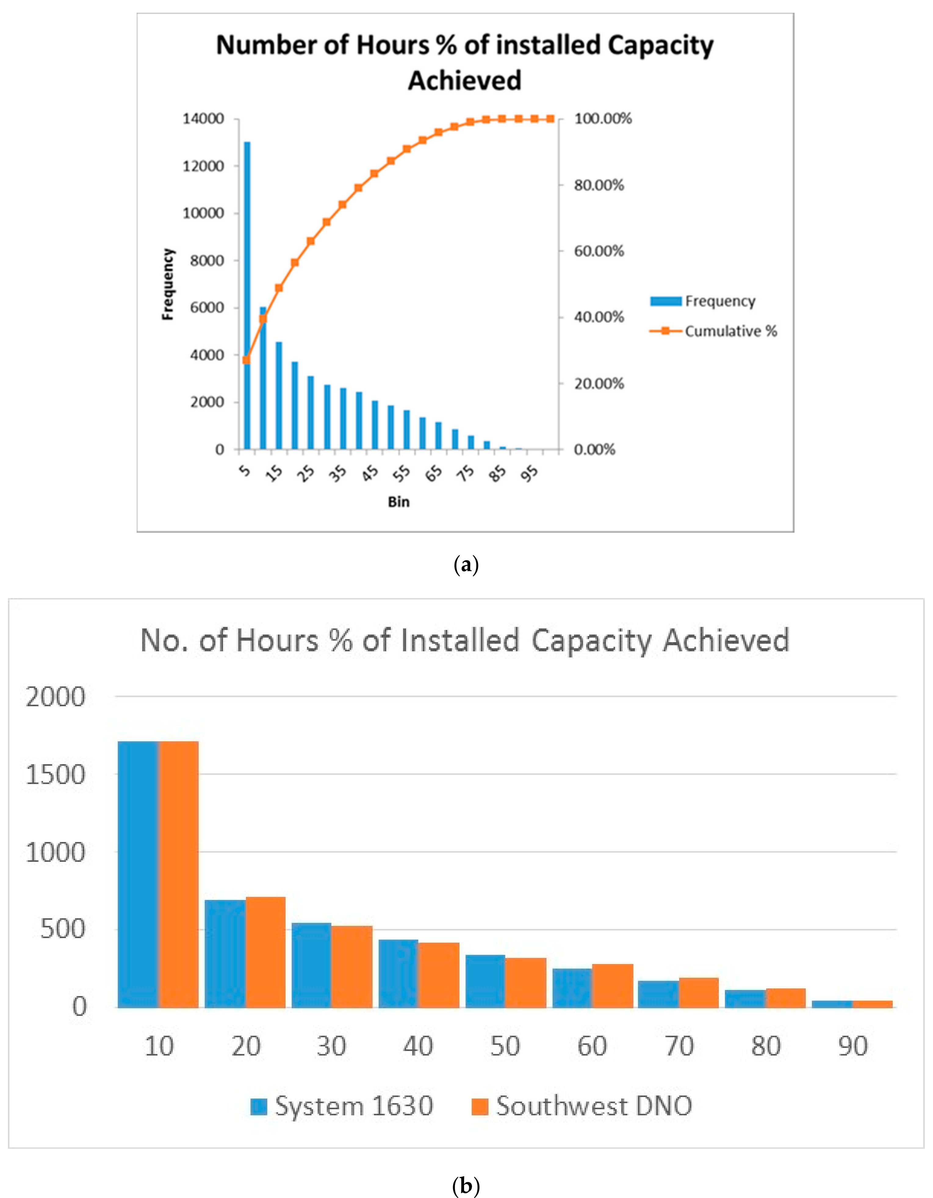
Most of the analysis so far has assumed that solar farms achieve their stated capacity. This section examines the prospect of this actually happening. Figure 12 indicates that, in fact, achievement of full capacity is unlikely on a national scale. Looking at a single year of solar farm output (2014) clarifies this. Figure 17a shows that less than 5% of large scale installed solar capacity was achieved for a quarter of 2014 (13,000 h out of approximately 5000 daylight hours multiplied by 11 DNO areas = 55,000 productive hours for all UK solar farms). No more than 93% capacity was ever realized in 2014. Figure 17b illustrates variation in frequency of achievement of installed capacity of an entire DNO (the Southwest) and the largest solar farm in that area (40.1 MW).
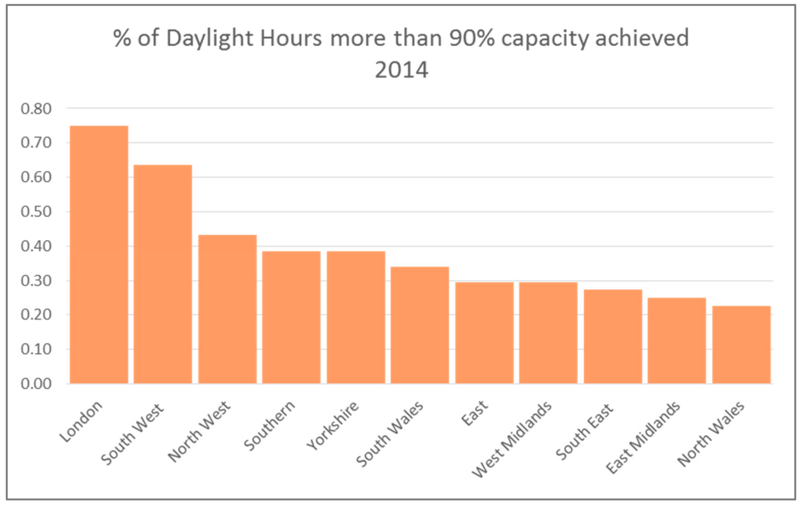
Figure 18 magnifies the 95% capacity bin of Figure 17a and looks at individual DNO areas to show how rarely high capacity output is attained.
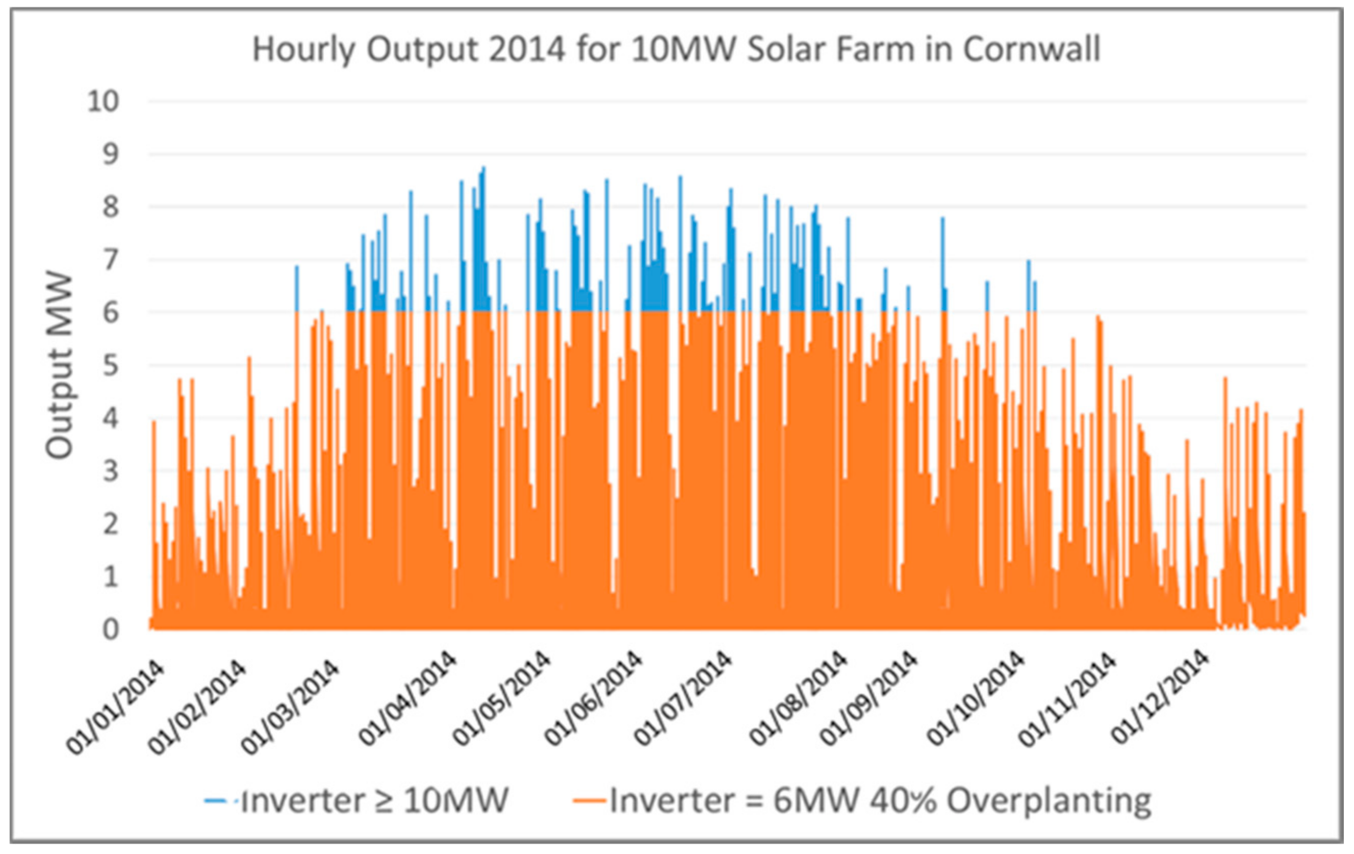
Despite these findings, some solar farm operators claim their installations frequently achieve full capacity. The explanation lies in how capacity is defined. Nameplate capacity or rated output is the datasheet module power output under internationally standardized (and fairly optimistic) test conditions, multiplied by the number of modules in the plant. But some solar energy companies use inverter datasheet rating to define capacity. Recently, falling module costs have led to oversizing or overplanting [23,24]. For instance, a 10 MW nameplate capacity Cornish solar farm is allocated a 6 MW inverter. The inverter must then engage in power limiting for considerable lengths of time, as opposed to little or none in the first scenario. Power limiting or clipping (from the flattening effect on the output graph) is when the available power is greater than the inverter’s rated input power and is down regulated to match. Inverters clip at times of peak array output. Figure 19 expands on this scenario. The 6 MW inverter capacity is achieved for 333 midday hours 16 February to 7 October (8% of annual sun hours). In comparison, the 10 MW nameplate capacity is never achieved for this solar farm. Relative to stated capacity, overplanted systems produce a greater annual yield but also result in peak clipping.
The object is to maximize power output for a given permitted installation capacity. If a DNO allows a 6 MW solar installation to be connected to its network, the solar farm operator has two permissible options. The first option is to install a 6 MW solar farm with a 6 MW inverter. Full 6 MW output is seldom or never achieved. The second option is to install a 10 MW solar farm with a 6 MW inverter. 6 MW output is achieved for 8% of annual sun hours (as explained above). Both options are declared to the DNO as 6 MW solar farms but the second injects far more power into the local transmission lines than the first. Although the solar farm operator has invested in 4 MW of panels for which power can only be utilized as for irradiances below 600 W/m (i.e., they are subject to power limiting or curtailment), overall more energy is supplied (and sold).
Connection of a generation plant to distribution networks of licensed DNOs is controlled by the Energy Network Association Engineering Recommendation G59 [25]. The relevant form asks for the maximum system output on the AC side in MW and is simply given by the combined rated AC output of the inverters. This is the maximum possible injection to the grid, which is their concern, and there is no requirement to give details of oversizing. Thus, there is no publicly available information as to whether the inverters for a given solar farm are likely to be clipping or not.
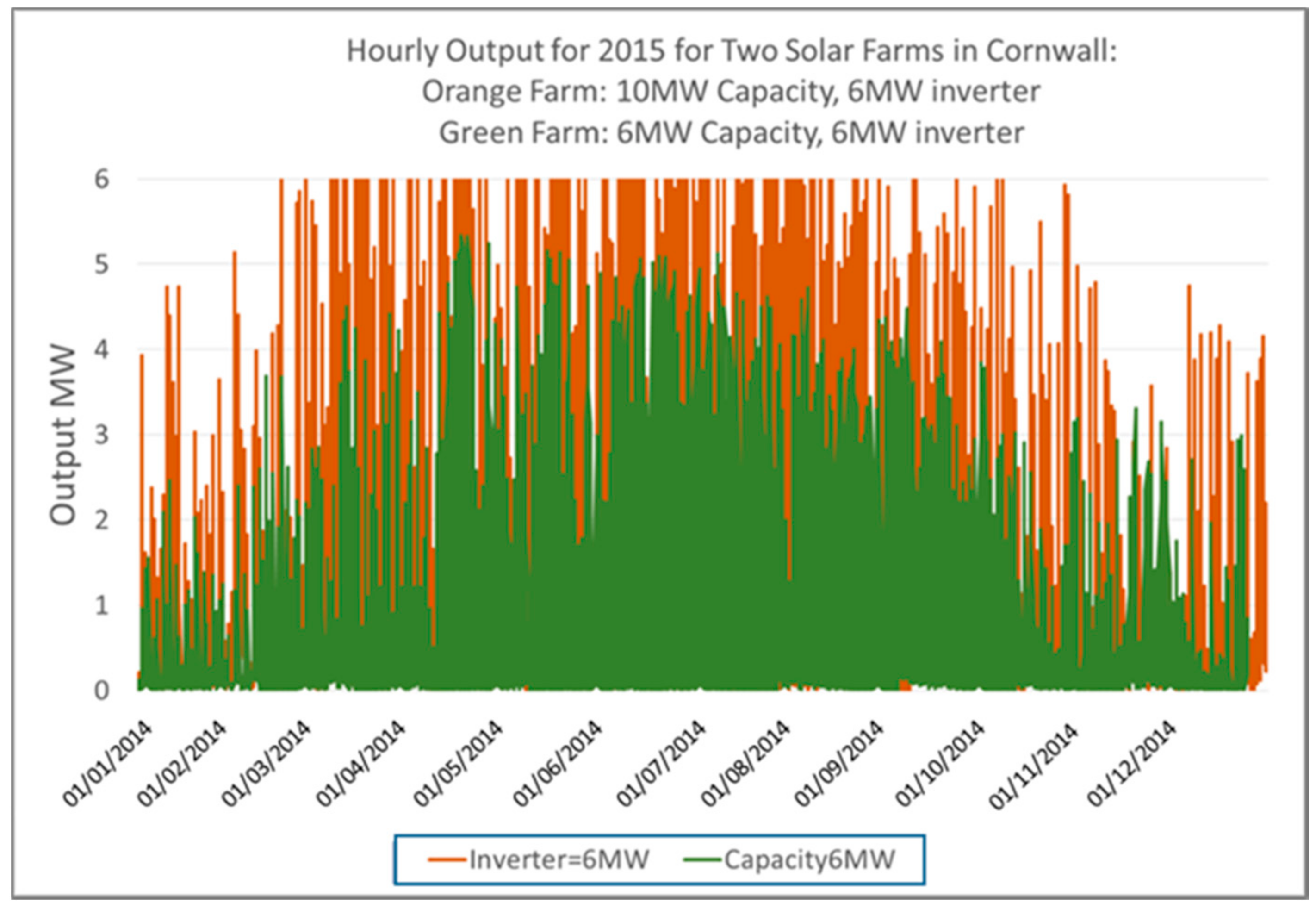
Hence, the installed capacity in the Renewable Energy Planning database does not take account of array-to-inverter ratios. Some of the solar farms oversize by up to 40% and some do not oversize at all. Therefore, planning for voltage control becomes difficult. The consequences of overplanting for annual yield are made clear in Figure 20. This graphs the output in MW of two Cornish solar farms. The 6 MW solar farm does not oversize and its output never approaches nameplate capacity throughout the year (2015). The 10 MW nameplate capacity solar farm has a 6 MW inverter. Therefore, its array-to-inverter ratio is 1.66 and it is oversizing by 40%. 6 MW output is achieved for 8% of annual sun hours.
4.4. Flexibility of UK Generation and Functioning of the UK Electricity Market
It has been demonstrated that occurrence of maximum yield from PV in the UK may be largely predicted. However, operational flexibility is helpful for integration of solar energy into the grid. Gas generation can supply this flexibility [26,27]. The most recent figures show that 30% of the UK’s electricity generation comes from gas [28] and this trend is increasing [29].
Analysis by the Solar Trade Association has shown that currently the cost of PV integration into the power generation system, including alternative generation for periods when PV is non-productive, is small (£1.30/MWh) [30]. Storage of energy in large quantities is still under development, so supply and demand of electricity of the UK is managed by the “Balancing Mechanism” [31]. Balancing comprises each power generator bidding to provide or withhold generation for half-hour time-slots in advance. Acceptance of bids is made on a basis of geographic location, speed of response and price. PV production fits into the “Balancing Mechanism” as follows. Contracts for Difference (CfDs) are awarded to renewable generators. Under these, PV suppliers receive an agreed price for their electricity, regardless of market price. Under the Energy Act 2013, CfD and non-CfD (largely non-renewables) holders are paired in a “capacity market”. The non-renewable generator is paid to generate or come off-line to support the fluctuating supply of the CfD [32]. This system enables PV to enter into the UK electricity market, whilst ensuring security of supply.
5. Conclusions
This paper opposes the conventional view that solar energy production may transcend the transmission capability of the UK National Grid. This fact is not presupposed but scientifically investigated and countered. The problem is often presented based on annual solar power production figures and national averages. This research provides a simulation of hour-by-hour generation for each individual utility-scale solar installation. Generation is compared to nearby grid capacity and local demand. Data has been aggregated to deliver a tool to determine the output of PV systems in the UK. Both spatial and temporal fluctuations in yield were studied, together with percentage of time full capacity and impact on the transmission network. This tool provides information on when, where, and if large scale solar installations stress grid capacity. Furthermore, it may be used to model future installation scenarios, using prospective capacity and fraction of peak output.
Perceived grid stresses may be investigated from four viewpoints: DNO/GSP area with highest number of solar farms or highest solar farm capacity, greatest distance to nearest GSP, or imbalance of supply and demand. The capacity of solar farms is of greater significance than their number, because in some areas a few large farms have the capability to produce more electricity than many smaller installations in nearby regions. It has been shown that modelling of output from nameplate rating gave 0% full capacity for 2014. Due to overplanting, attainment of capacity will actually lie somewhere above this, e.g., 5% of hours when down-regulation is potentially required. In practice, this represents very little impact on the UK National Grid.
Long distances between the generator and the nearest grid connection point may stress local networks. This is not perceived as a hazard in the UK because the majority of solar farms are within 10 km of high voltage transmission lines. Imbalance of supply and demand could cause instabilities in all voltage layers. Demand and production is not well-balanced for UK solar farms. However, the timing of output may be anticipated. Maximum yield occurs at predictable times (middle of the day, March–September). Smoothing of grid insertion is also apparent. Solar farm output varies according to geographic position (east/west), hour of day, and time of year. April solar farm output may equal that of June. The most productive hour of the day is also one of the most variable.
Case studies have strongly suggested that there is plenty of capacity on the grid for additional solar farm production. Potential grid overload may be seen as a risk in different localities, dependent on how it is assessed, so the hypothetical stresses on the network may not arise solely in Cornwall.
Overall, it has been demonstrated that there is little threat to the grid from solar farm output at the current time. Variability of production depends strongly on weather patterns. The UK differs in this respect to other European countries, as well as in its network structure. More accurate modelling can be performed if information on solar farm inverter sizes becomes available.
Supplementary Materials
Supplementary materials can be found at www.mdpi.com/1996-1073/10/8/1220/s1.
Acknowledgments
This work was started as part of the research project “PV2025—Potential Costs and Benefits of Photovoltaic for UK Infrastructure and Society” project which is funded by the RCUK’s Energy Programme (contract No.: EP/K02227X/1). It was continued under ‘Joint UK-India Clean Energy Centre (JUICE)’, funded by the RCUK's Energy Programme (contract no: EP/P003605/1). The projects funders were not directly involved in the writing of this article.
Author Contributions
Diane Palmer, Tom Betts and Ralph Gottschalg conceived and designed the experiments; Diane Palmer and Elena Koubli analyzed the data; Elena Koubli contributed data; Diane Palmer wrote the paper.
Conflicts of Interest
The authors declare no conflict of interest.
Appendix A
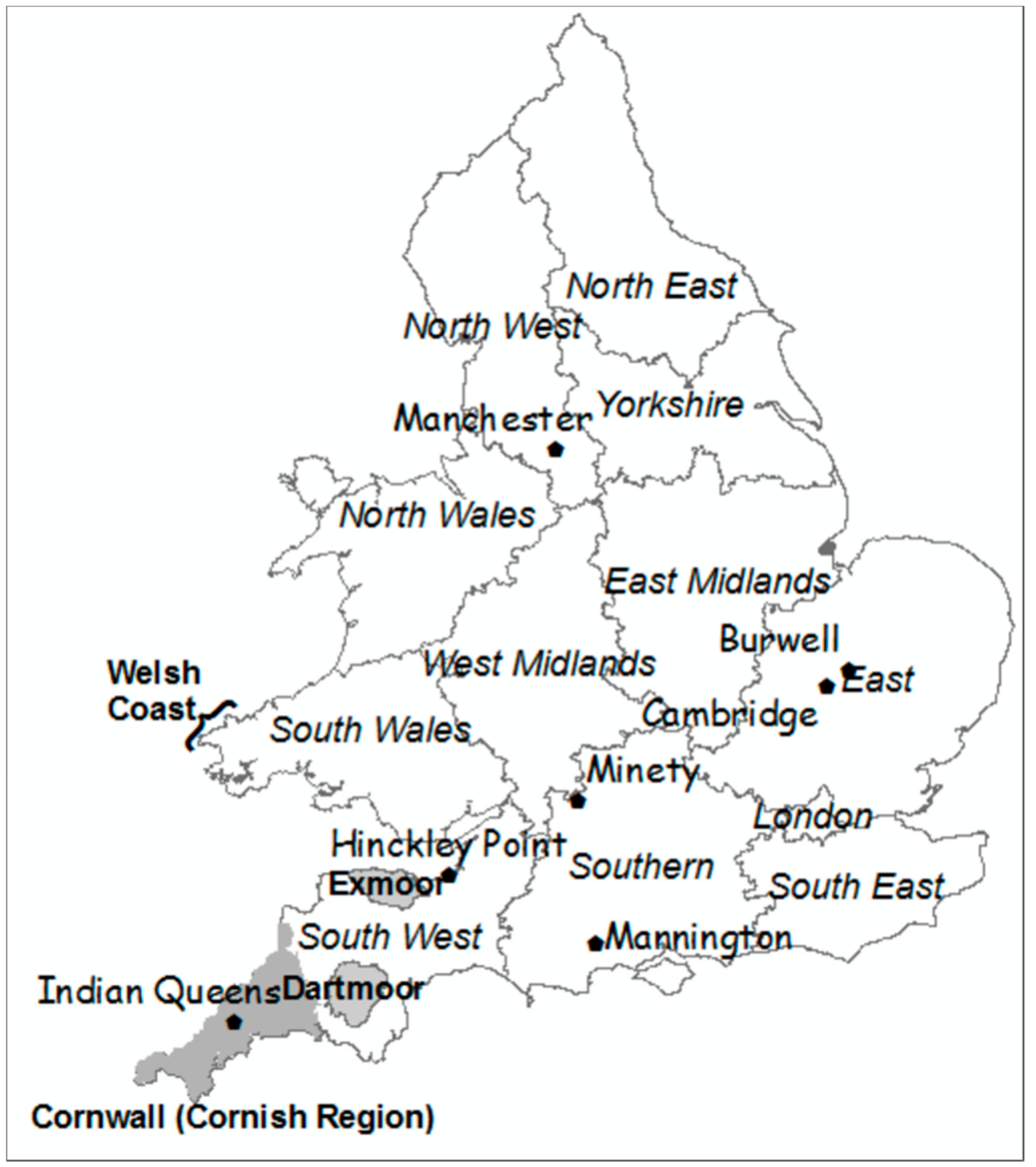
Figure A1.
Map showing locations of all UK areas, cities and towns covered by this research.

References
- Department of Energy and Cliimate Change (DECC). UK Solar PV Strategy Part 1: Roadmap to a Brighter Future. Available online: https://www.gov.uk/government/publications/uk-solar-pv-strategy-part-1-roadmap-to-a-brighter-future (accessed on 8 June 2017).
- Germany’s Power Grid under Increasing Pressure. Oil Drum, 2012. Available online: http://oilprice.com/Energy/Energy-General/Germanys-Power-Grid-under-Increasing-Pressure.html (accessed on 2 May 2017).
- Hepworth, A. Rooftop Solar Panels Overloading Electricity Grid. The Australian, 2011. Available online: http://www.theaustralian.com.au/news/rooftop-solar-panels-overloading-electricity-grid/news-story/5ea583571dde0830ec34d3cd8c32b9dc (accessed on 2 May 2017).
- Western Power Distribution. WPD South West Network Capacity Restriction. March 2015. Available online: https://www.westernpower.co.uk/docs/connections/Generation/Generation-capacity-map/Distributed-Generation-EHV-Constraint-Maps/WPD-South-West-network-capacity-restriction.aspx (accessed 3 May 2017).
- DECC. Renewable Energy Planning Database Monthly Extract. 2015. Available online: https://www.gov.uk/government/publications/renewable-energy-planning-database-monthly-extract (accessed 30 September 2015).
- UK Met Office. MIDAS: Global Radiation Observations. NCAS British Atmospheric Data Centre, 2006. Available online: http://catalogue.ceda.ac.uk/uuid/b4c028814a666a651f52f2b37a97c7c7 (accessed on 17 August 2016).
- Palmer, D.; Cole, I.; Betts, T.; Gottschalg, R. Interpolating and estimating horizontal diffuse solar irradiation to provide UK-wide coverage: Selection of the best performing models. Energies 2017, 10, 181. [Google Scholar] [CrossRef]
- Hofstra, N.; Haylock, M.; New, M.; Jones, P.; Frei, C. Comparison of six methods for the interpolation of daily, European climate data. J. Geophys. Res. Atmos. 2008, 113. [Google Scholar] [CrossRef]
- Palmer, D.; Koubli, E.; Cole, I.; Betts, T.; Gottschalg, R. Satellite or ground-based irradiation data: Which is closer to reality? In Proceedings of the 13th Photovoltaic Science, Applications and Technology Conference, Bangor, UK, 5–7 April 2017. [Google Scholar]
- Ridley, B.; Boland, J.; Lauret, P. Modelling of diffuse solar fraction with multiple predictors. Renew. Energy 2010, 35, 478–483. [Google Scholar] [CrossRef]
- Hay, J.E.; Perez, R.; McKay, D.C. Estimating solar irradiance on inclined surfaces: A review and assessment of methodologies. Int. J. Sol. Energy 1986, 4, 321–324. [Google Scholar] [CrossRef]
- Reindl, D.T.; Beckman, W.A.; Duffie, J.A. Evaluation of hourly tilted surface radiation models. Sol. Energy 1990, 45, 9–17. [Google Scholar] [CrossRef]
- Ross, R.G. Interface design considerations for terrestrial solar cell modules. In Proceedings of the 12th Photovoltaic Specialists Conference, Baton Rouge, LA, USA, 15–18 November 1976; pp. 801–805. [Google Scholar]
- Kratochvil, J.A.; Boyson, W.E.; King, D.L. Photovoltaic Array Performance Model. SAND2004-3535; 2004. Available online: http://prod.sandia.gov/techlib/access-control.cgi/2004/043535.pdf (accessed on 3 May 2017).
- Koubli, E.; Palmer, D.; Rowley, P.; Gottschalg, R. Inference of missing data in photovoltaic monitoring datasets. IET Renew. Power Gener. 2016, 10, 1–6. [Google Scholar] [CrossRef] [Green Version]
- Carrington, A.; Rahman, N.; Ralphs, M. The Modifiable Areal Unit Problem: Research Planning. 11th Meeting of the National Statistics Methodology Advisory Committee. 2006. Available online: https://www.ons.gov.uk/ons/guide-method/method-quality/advisory-committee/2005-2007/eleventh-meeting/the-modifiable-areal-unit-problem--research-planning.pdf (accessed on 3 May 2017).
- National Grid. Shape Files, National Grid. Available online: http://www2.nationalgrid.com/uk/services/land-and-development/planning-authority/shape-files/ (accessed on 28 September 2016).
- ET Geo Wizards. Build Thiessen Polygons. Available online: http://www.ian-ko.com/ET_GeoWizards/UserGuide/thiessenPolygons.htm (accessed on 5 June 2017).
- National Grid. Electricity Ten Year Statement (ETYS), National Grid. 2015. Available online: http://www2.nationalgrid.com/UK/Industry-information/Future-of-Energy/Electricity-Ten-Year-Statement/ (accessed on 30 September 2016).
- Richardson, I. Integrated High-Resolution Modelling of Domestic Electricity Demand and Low Voltage Electricity Distribution Networks. Ph.D. Thesis, Loughborough University, Loughborough, UK, 2011. [Google Scholar]
- Scottish and Southern Energy Power Distribution (SSEPD). Generation Availability Map. Available online: https://www.ssepd.co.uk/GenerationAvailabilityMap/?mapareaid=1 (accessed on 30 September 2016).
- Western Power Distribution (WPD) South West 132 kV Network Capacity Restriction UPDATE March 2016. Available online: https://www.westernpower.co.uk/docs/connections/Generation/Generation-capacity-map/Distributed-Generation-EHV-Constraint-Maps/WPD-South-West-F-Route-Constraint-Information-Marc.aspx (accessed on 3 May 2017).
- United States Nuclear Regulatory Commission. NRC: Glossary-Generator Nameplate Capacity. 2016. Available online: http://www.nrc.gov/reading-rm/basic-ref/glossary/generator-nameplate-capacity.html (accessed 3 October 2016).
- Fiorelli, J.; Zuercher-Martinson, M. How oversizing your array-to-inverter ratio can improve solar-power system performance. Sol. Power World 2013, 7, 42–48. [Google Scholar]
- Energy Networks Association. Distributed Generation Connection Guide. Available online: http://www.energynetworks.org/assets/files/DGCG%20G59%20Full%20April%20%202016v1.pdf (accessed on 3 May 2017).
- Raugei, M.; Leccisi, E. A comprehensive assessment of the energy performance of the full range of electricity generation technologies deployed in the United Kingdom. Energy Policy 2016, 90, 46–59. [Google Scholar] [CrossRef]
- Clegg, S.; Mancarella, P. Integrated electrical and gas network flexibility assessment in low-carbon multi-energy systems. IEEE Trans. Sustain. Energy 2016, 7, 718–731. [Google Scholar] [CrossRef]
- Department for Business, Energy & Industrial Strategy (DBEIS). Digest of UK Energy Statistics (DUKES). Available online: https://www.gov.uk/government/collections/digest-of-uk-energy-statistics-dukes (accessed on 15 August 2017).
- DBEIS. Energy Trends. June 2017. Available online: https://www.gov.uk/government/uploads/system/uploads/attachment_data/file/622841/Energy_Trends_June_2017.pdf (accessed on 15 August 2017).
- Aurora Energy Research. Intermittency and the Cost of Integrating Solar in the GB Power Market. Available online: http://www.solar-trade.org.uk/intermittency-cost-integrating-solar-gb-power-market/ (accessed on 15 August 2017).
- Hassan, M.; Majumder-Russell, D. Electricity Regulation in the UK: Overview. Available online: https://uk.practicallaw.thomsonreuters.com/1-523-9996?transitionType=Default&contextData=(sc.Default)&firstPage=true&bhcp=1#co_anchor_a514191 (accessed on 15 August 2017).
- Office of Gas and Electricity Markets (Ofgem). The GB Electricity Wholesale Market. Available online: https://www.ofgem.gov.uk/electricity/wholesale-market/gb-electricity-wholesale-market (accessed on 15 August 2017).
Figure 1.
Summary of stages involved in generation of solar farm output.

Figure 2.
Construction of grid supply point (GSP) areas using Thiessen polygons.

Figure 3.
Solar farms, high voltage power lines, and large urban areas in the UK. (a) Solar farms compared to location of high voltage lines; (b) size of solar farms.
Figure 3.
Solar farms, high voltage power lines, and large urban areas in the UK. (a) Solar farms compared to location of high voltage lines; (b) size of solar farms.

Figure 4.
Average annual global horizontal irradiation of each DNO, kWh/m2 (ten-year average 2005–2014). (a) Average annual GHI per DNO, kWh/m2; (b) interpolated irradiance (blue = low, orange = high).
Figure 4.
Average annual global horizontal irradiation of each DNO, kWh/m2 (ten-year average 2005–2014). (a) Average annual GHI per DNO, kWh/m2; (b) interpolated irradiance (blue = low, orange = high).

Figure 5.
Number and total capacity of UK solar farms in 2015.

Figure 6.
Modelled annual output for solar farms 2014, MWh.

Figure 7.
Solar farms per GSP 2015. (a) Number; (b) capacity in MW.

Figure 8.
Calculated solar farm output in 2014 allocated to GSP area/point compared to electricity ten-year statement GSP winter peak demands 2015 (Demand data obtained from [19]. (a) Solar farm output allocated to GSP area MW 2014; (b) Demand per GSP area MW 2015; (c) Solar farm output and demand per GSP point (background DNO areas).

Figure 9.
Calculated overloads compared to DNO company constraints on BSP in Southern DNO. (a) Total capacity of solar farms per BSP Thiessen polygon; (b) overloads and constraints on BSPs.
Figure 9.
Calculated overloads compared to DNO company constraints on BSP in Southern DNO. (a) Total capacity of solar farms per BSP Thiessen polygon; (b) overloads and constraints on BSPs.

Figure 10.
Solar farms and high voltage line in restricted Southwest region.

Figure 11.
Frequency of 2014 power output normalized by average annual output for 4 VW solar farms for largest site and all sites.
Figure 11.
Frequency of 2014 power output normalized by average annual output for 4 VW solar farms for largest site and all sites.

Figure 12.
Percentage of daylight hours in each fraction of peak output bin (2005–2014).

Figure 13.
Average fraction of peak output per hour (2005–2014).

Figure 14.
Boxplots illustrating Variability of average hourly fraction of peak output (5: 00 am–8: 00 pm) for each DNO (2005–2014).
Figure 14.
Boxplots illustrating Variability of average hourly fraction of peak output (5: 00 am–8: 00 pm) for each DNO (2005–2014).

Figure 15.
Average hourly fraction of output on a daily basis (2005–2014).

Figure 16.
Boxplots illustrating variability of average monthly fraction of output for each DNO (2005–2014).
Figure 16.
Boxplots illustrating variability of average monthly fraction of output for each DNO (2005–2014).

Figure 17.
Number of hours during which output reaches a given percentage of installed capacity (capacity shown as bins). (a) By 575 solar farms countrywide 2014; (b) by single solar farm 1630 and 175 solar farms in Southwest DNO.
Figure 17.
Number of hours during which output reaches a given percentage of installed capacity (capacity shown as bins). (a) By 575 solar farms countrywide 2014; (b) by single solar farm 1630 and 175 solar farms in Southwest DNO.

Figure 18.
Percentage of daylight hour more than 90% capacity achieved by UK solar farm fleet 2014.

Figure 19.
Effect of overplanting/power limiting, e.g., 6 MW inverter for 10 MW nameplate capacity solar farm.
Figure 19.
Effect of overplanting/power limiting, e.g., 6 MW inverter for 10 MW nameplate capacity solar farm.

Figure 20.
Effect of overplanting portrayed by two solar farms in Cornwall—one overplanted by 40%, the other equal capacity inverter and field.
Figure 20.
Effect of overplanting portrayed by two solar farms in Cornwall—one overplanted by 40%, the other equal capacity inverter and field.


Table 1.
Alternative solutions to the Modifiable Area Unit problem (MAUP) for solar farms aggregated by distribution network operator (DNO) area.
Table 1.
Alternative solutions to the Modifiable Area Unit problem (MAUP) for solar farms aggregated by distribution network operator (DNO) area.
| Technique | Details | Advantages | Disadvantages |
|---|---|---|---|
| Centre point | Use irradiation of the centre point of the DNO area (or use the solar farm location nearest to the centre) | Latitude of specific point used for calculating POA irradiation data | Single central point taken as representative of area; better than solar farm average (below) because of central location of point but MAUP is still a risk |
| DNO average | Obtain the average irradiation of the DNO by averaging all interpolated values falling inside the DNO area | Overcomes MAUP | Averaged input supplied to POA algorithm can cause unrealistic results |
| Solar farm average | Obtain temperature and irradiation from nearest grid point to solar farm | Uses exact locations; POA algorithm uses correct latitudes | Just a few points are taken as representative of the whole area (MAUP occurs); delivers obviously “wrong” results; e.g., Yorkshire with highest irradiation |
| Central weather station | Take the irradiation of the Weather Station closest to the DNO area centre. (no interpolation involved) | Overcomes MAUP; easy to understand; fast processing; uses exact locations; POA algorithm uses correct latitudes | Some DNOs have no central weather station; necessitates choosing a peripheral one; single central point taken as representative of area; MAUP is still a risk |
Table 2.
Results of applying alternative solutions to MAUP in Southwest DNO.
| Hourly Global Horizontal Irradiance | Solar Farm Furthest from DNO Centre | Centre Point | DNO Average | Average of Solar Farms in DNO | Central Weather Station |
|---|---|---|---|---|---|
| Maximum hourly GHI in 2014 (Wh/m2) | 900 | 931 | 932 | 855 | 992 |
| Mean hourly GHI in 2014 (Wh/m2) | 219 | 221 | 221 | 219 | 236 |
| Standard deviation of hourly GHI in 2014 (Wh/m2) | 218 | 216 | 216 | 203 | 223 |
© 2017 by the authors. Licensee MDPI, Basel, Switzerland. This article is an open access article distributed under the terms and conditions of the Creative Commons Attribution (CC BY) license (http://creativecommons.org/licenses/by/4.0/).
Share and Cite
MDPI and ACS Style
Palmer, D.; Koubli, E.; Betts, T.; Gottschalg, R. The UK Solar Farm Fleet: A Challenge for the National Grid? †. Energies 2017, 10, 1220. https://doi.org/10.3390/en10081220
AMA Style
Palmer D, Koubli E, Betts T, Gottschalg R. The UK Solar Farm Fleet: A Challenge for the National Grid? †. Energies. 2017; 10(8):1220. https://doi.org/10.3390/en10081220
Chicago/Turabian StylePalmer, Diane, Elena Koubli, Tom Betts, and Ralph Gottschalg. 2017. "The UK Solar Farm Fleet: A Challenge for the National Grid? †" Energies 10, no. 8: 1220. https://doi.org/10.3390/en10081220
Note that from the first issue of 2016, this journal uses article numbers instead of page numbers. See further details here.