An Intelligent Hybrid Heuristic Scheme for Smart Metering based Demand Side Management in Smart Homes
by
 , , , and
Awais Manzoor
1, 
Nadeem Javaid
1,* ,
,
Ibrar Ullah
2,
Wadood Abdul
3,
Ahmad Almogren
3 and
Atif Alamri
3 1
COMSATS Institute of Information Technology, Islamabad 44000, Pakistan
2
University of Engineering and Technology Peshawar, Bannu 28100, Pakistan
3
Research Chair of Pervasive and Mobile Computing, College of Computer and Information Sciences, King Saud University, Riyadh 11633, Saudi Arabia
*
Author to whom correspondence should be addressed.
Energies 2017, 10(9), 1258; https://doi.org/10.3390/en10091258
Submission received: 29 June 2017
/
Revised: 11 August 2017
/
Accepted: 16 August 2017
/
Published: 24 August 2017
(This article belongs to the Special Issue From Smart Metering to Demand Side Management)
Abstract
:Smart grid is an emerging technology which is considered to be an ultimate solution to meet the increasing power demand challenges. Modern communication technologies have enabled the successful implementation of smart grid (SG), which aims at provision of demand side management mechanisms (DSM), such as demand response (DR). In this paper, we propose a hybrid technique named as teacher learning genetic optimization (TLGO) by combining genetic algorithm (GA) with teacher learning based optimization (TLBO) algorithm for residential load scheduling, assuming that electric prices are announced on a day-ahead basis. User discomfort is one of the key aspects which must be addressed along with cost minimization. The major focus of this work is to minimize consumer electricity bill at minimum user discomfort. Load scheduling is formulated as an optimization problem and an optimal schedule is achieved by solving the minimization problem. We also investigated the effect of power-flexible appliances on consumers’ bill. Furthermore, a relationship among power consumption, cost and user discomfort is also demonstrated by feasible region. Simulation results validate that our proposed technique performs better in terms of cost reduction and user discomfort minimization, and is able to obtain the desired trade-off between consumer electricity bill and user discomfort.
1. Introduction
The conventional power grid is often considered as a complex machine ever built. The entire electrical network is composed of four main units: generation, transmission, distribution, and consumption. The conventional grid is capable of delivering the electrical power from generation unit to end consumer via transmission and distribution networks. The one-way communication infrastructure in the traditional grid is incapable to efficiently handle several parameters of the entire electrical network. The main deficiencies in the conventional grid are: incapable to optimally handle economic dispatch, unit commitment, state estimation, monitoring of transmission lines, faults detection, self-healing and managing the demand in real time environment [1].
In this regard, valuable research work has been carried out to address the aforementioned problems. As a result, the smart grid (SG) has emerged as a solution to overcome these limitations. SG integrates advanced metering infrastructure (AMI), a smart meter (SM), intelligent control system and advanced communication technologies. Integration of renewable energy sources (RESs), cost reduction and load management issues have attained the focus of many researchers regarding power management; which is considered to be the most crucial factor in order to fulfill the increasing power demand [2]. The management of power is classified into two categories. One is supply side management (SSM) and the other is demand side management (DSM). The former ensures efficient generation, transmission, and distribution of electricity. This is also responsible for providing reliable energy at minimum economic cost [3]. However, our work is focused on latter that aims at planning and monitoring activities [4,5]. Demand response (DR) is a component of DSM, which encourages consumers to modify their energy consumption pattern and shift their load from on-peak hours to off-peak hours. Cost sensitive consumers participate in DR by adjusting their power demand in response to time-varying prices.
A decentralized algorithm is proposed in [6] to optimally manage charging an discarding of electric vehicle (EV). In this framework, aggregator and consumers are considered as two entities in which aggregator maximizes the profit of utility while consumers minimize their electricity bill. Consumers manage their charging and discarding schedule in response to time-varying prices, which benefits not only consumers in minimizing their electricity bill but also keeps distribution of network within its operational limits. Vehicle-to-vehicle (V2V), vehicle-to-grid (V2G) and grid-to-vehicle (G2V) exchange of power is also considered by providing monetary incentives. In [7,8,9,10,11], mixed integer linear programming (MILP) is used to solve the problem of residential DR. A distributed network of RES along electric storage system (ESS) is also efficiently tackled, whereas penetration of EV for energy trading is also taken into consideration [7]. Authors in [8] analyzed two different scenarios, one of which is based on ripple control while the other is based on optimal load scheduling, showing that scheduling performs better in terms of cost reduction. D. Zhang et al. [9] dedicated their work to consumers’ bill and CO emission minimization, ignoring user comfort. In [10], authors mainly focused their work on task scheduling with thermal comfort constraints. RES and ESS have been efficiently integrated to fulfill consumers’ thermal comfort requirements. Shiftable, thermal and interruptible loads are considered in [11]. Shiftable loads have predefined working cycles while thermal loads have variable working cycles during different time slots. However, adopting day-ahead pricing (DAP) [7,8,9,10,11] scheme shows a large gap with hourly real-time price (RTP) due to estimation error [12].
Authors in [13] developed a home energy management system (HEMS) to determine an optimal load schedule. DR is applied for load-shaping under DAP for minimizing consumer’s electricity bill. Peak power limit restricts the load below the upper limit. Utilization of ESS is handled efficiently to meet the energy requirement of a consumer in on-peak hours. In [14], a multi-layer ant colony optimization (MACO) is used to solve the energy management problem in stand-alone microgrid. The microgrid consists of wind turbine (WT), photovoltaic (PV), microturbine (MT) and ESS. Results obtained from MACO are also compared with conventional EMS and particle swarm optimization (PSO). MACO shows better performance as compared to conventional EMS and PSO, due to fast convergence and less computational complexity. Similarly, authors in [15,16] used game theory approach to minimize consumers electricity consumption cost. Noncooperative multi-agent game theoretic approach is developed for managing demand of a group [15], while maximizing profit of both, utility and consumer. 0–1 mixed integer programming is utilized to compute non-dominated solutions. Algorithm developed in [16] is also based on noncooperative approach which uses dominance game strategy. However, user comfort is not addressed in all the aforementioned papers.
Customized evolutionary algorithm [17] is utilized for multi-objective optimization of residential loads. Thermostatically controlled loads and shiftable loads are considered for scheduling. The multi-objective model considers cost and user dissatisfaction minimization as objective functions. Optimal stopping rule (OSR) [18] is applied to schedule home appliances based on RTP. The problem is formulated to minimize energy consumption cost, considering technical operational constraints of appliances. Different duty cycles of the appliances are scheduled e.g., ice making and defrost cycles. OSR works on threshold based policy, which is the major limitation of this work. If price does not fall below the threshold then appliances will remain in waiting state.
Several aspects must be considered in order to achieve a coordination between utility and consumer, such as, cost minimization, operational issues, load balance and user satisfaction. User satisfaction is one of the important aspects which must be considered along with electricity bill reduction. Nature-inspired optimization techniques are able to efficiently address these complex tasks in load scheduling problems.
The aim of this work is to design an intelligent HEMS for a single home which can effectively schedule consumers’ power demand. We have applied three existing optimization techniques: genetic algorithm (GA), teacher learning-based optimization (TLBO) and linear programming (LP). We also proposed a teacher learning genetic optimization (TLGO) by combining GA with TLBO to achieve our objectives i.e., to minimize cost with minimum user discomfort. We compared the performance of heuristic techniques with LP in terms of cost, peak power consumption, peak to average ratio (PAR) and user discomfort. Our major contribution is to minimize consumers’ electricity bill at minimum user discomfort.
Rest of the paper is organized as follows: Section 2 reviews state-of-the-art work. Problem description is given in Section 3 and problem is formulated in Section 4. System model is described in Section 5 and proposed solution is given in Section 6. Simulations and discussions are presented in Section 7 and finally, Section 8 contains the concluding remarks of our work.
2. Related Work
In literature, many optimization techniques are presented for load scheduling to reduce consumer electricity bill and peak power demand reduction. HEMS has an important role in residential load scheduling. Rastegar et al. [19] proposed DR-based HEMS for residential sector to minimize consumer electricity bill while maximizing user comfort. Appliances are categorized into two categories: controllable and uncontrollable appliances. For optimal scheduling of household electrical appliances, time of use (ToU) and inclined block rate (IBR) pricing schemes are applied. Operational priority of controllable appliances is also taken into consideration to maximize user comfort. The value of load loss (VOLL) is calculated to determine the priority of running an appliance at any specific time slot. Proposed solution reduces the cost and maximizes user comfort, however, PAR is ignored.
In [20], authors utilized interval number optimization for scheduling of household appliances. Appliances are categorized into interruptible, non-interruptible and thermostatically controlled load. Interval number analysis is introduced for handling uncertain hot water demand and ambient temperature. Binary PSO (BPSO) combined with integer linear programming (ILP) is used for load scheduling to minimize consumers’ electricity bill; while thermal comfort is also taken into consideration.
Shirazi and Jadid [21] proposed a residential power scheduling technique to coordinate appliances and distributed energy resources (DERs). Scheduling is performed under DAP for shifting the load from on-peak hours to off-peak hours. Mixed integer nonlinear programming (MINLP) is used to formulate the multi-objective function. The optimization problem is solved for two conflicting objectives, i.e., to minimize energy consumption cost and maximize user comfort. Authors considered both electrical and thermal appliances for scheduling. Proposed technique is analyzed for summer and winter under different scenarios. Results show the reduction of 1.5% to 1.8% in cost by reducing hot water temperature by 1 C; however, MINLP has high computational complexity.
Automated DR is applied in [22] for solving cost minimization problem via MINLP, while minimizing daily power consumption. Home appliances are classified into five categories including electrical and thermal appliances. High prices are applied when consumers’ demand exceeds the threshold, which helps to avoid peak creation in off-peak hours.
In [23], the grid and RES are considered as two main energy sources. Energy trading is also handled where a consumer can sell surplus energy to the others. Authors addressed load scheduling problem along with the exchange of power among different consumers and utility. Approximate dynamic programming technique is used for load scheduling purpose whereas game theory is applied to tackle the power exchange among different consumers. In this way, the proposed scheme has successfully managed to reduce the electricity consumption cost. Moreover, due to the distribution of energy among consumers, the reverse flow of energy is also reduced, which increase the stability of the entire grid. Zhao et al. [24] integrated RES and plug-in electric vehicle (PHEV) where surplus electricity can be sold back to the grid. Authors presented distributed optimization algorithm to minimize consumers’ electricity bill and achieved a flattened load curve.
Chakraborty et al. [25] presented a model for energy optimization by integrating PV and a wind turbine as RES. Fuzzy logic is used to address uncertainties caused by integration of RES. An intelligent quantum evolutionary algorithm (EA) is implemented for scheduling and dispatching of electricity, considering economic and environmental aspects. Resource scheduling is handled in an excellent way to reduce carbon emissions and production cost. Rajalingam and Malathi [26] developed the smart controller for HEMS to minimize electricity bill and peak power demand. Solar power is a primary source of energy while in the case of unavailability of solar power, controller shifts to the grid. Selective harmonic elimination method is presented to handle power quality disturbance resulted from DC to AC conversion. Results show the saving of 90 units/month from the grid and this requirement is fulfilled from PV generated energy.
In [27], a multi-objective EA is proposed with the objectives to minimize cost and waiting time. Appliances are temporarily stopped when total running load exceeds the predefined limit, which restrict the load within a limit. Integration of wind energy with ESS is proposed in [28] to minimize carbon emissions. DR is implemented to reduce cost, carbon emissions and to increase utilization of wind energy. The multi-objective function is converted into a single objective by linear combination through weighted sum method. Different case studies are taken to validate the proposed solution. Results show that incorporating DR and ESS decrease both consumers bill and carbon emissions while maximizing the utilization of wind energy.
An energy scheduling mechanism is proposed in [29] to minimize energy consumption cost by considering energy prices and comfort constraints. For comfort management, energy scheduler adjust the temperature of a room from the given range of temperature according to user preferences. Wireless sensors are utilized to measure the temperature and pass this information to the control system. Based upon temperature and pricing information, scheduler controls the Heating, ventilation, and air conditioning (HVAC) operation by the use of actuators. Objective function is formulated as a convex combination of energy consumption cost and penalty factor, reflecting consumers’ comfort constraints. In [30], multi-objective MILP is applied for managing energy in a smart home by considering both energy saving and consumers’ termal comfort. Integration of RES and task scheduling is efficiently handled in order to maximize the usage from RES. Authors of [29,30] have not considered time-shiftable appliances in their work. Quality of experience (QoE) aware smart HEMS proposed in [31], relies on annoyance suffered by users due to the change with respect to user preferences. Smart HEMS relies on two algorithm: QoE aware cost saving appliance scheduling (Q-CSAS) and QoE aware renewable source power allocation (Q-RSPA). The Former handles the scheduling of controllable load, based on users’ profile and electricity prices, whereas the latter changes the schedules according to availability of the renewable sources. Major contribution of [30,31] is to jointly optimize DER and main grid power usage by considering uncertainties caused by DER and cost variations of the power grid. However, the model in [31] is based on greedy approach which considers immediate solution, ignoring the long-term benefits. Therefore, the greedy algorithm does not always provide optimal solution.
A framework for DSM is presented in [32] with a concept of load clustering. Appliances’ power consumption pattern is predicted based on historical data. The aggregator is used to coordinate the power request of appliances. DAP is applied to synchronize charging and discharging pattern and to get the cost effective power consumption pattern. A model for optimal power flow is presented in [33], with an objective function of cost minimization and power balance under ToU pricing scheme. Integration of RES and ESS is also handled efficiently where the consumers have flexibility to sell surplus electricity back to the grid. Three main components of the cost function are: first, electricity purchasing cost from the grid, second, revenue generated from selling electricity to the grid and the third is installation cost of the hybrid system.
Vardakas et al. [34] analyzed different power demand scheduling scenarios for reducing peak demand. Fixed, power compressible and time-shiftable appliances are taken into consideration. Authors analyzed four different scenarios to minimize peak load demand during on-peak hours. The major achievement of this work is the proposed recursive formula which is used to determine the distribution of power units in use. However, the assumption of infinite number of appliances result in overestimation. To overcome the aforementioned limitation, authors extended their work for finite number of appliances [35]. A residential area with 50 homes is assumed where each home has same appliances. Four scenarios are analyzed to minimize peak demand load. Each scenario is associated with RTP, which provides incentives to the users for compressing their power demands.
GA is used by Bharathi et al. [36] to minimize power consumption in residential, commercial and industrial area. Authors also compared the performance of GA with other EAs. Result shows an overall reduction of 21.9% in power consumption during on-peak hours. Gupta et al. [37] applied GA for solving cost minimization problem. Authors formulated the problem via MILP, while GA is applied to determine the schedule. Integration of RES along with ESS is handled efficiently to modify consumers’ load profile. There is also a mechanism where excessive energy can be sold back to the grid. Authors in [38] presented their model for HEMS with an objective to minimize cost while maximizing user comfort in terms of minimizing appliances waiting time. The proposed model is based upon evolutionary techniques (GA, BPSO and cukko search). Authors also evaluated their model with and without integration of RES. Results shows a significant cost saving, however power-flexible appliances are not considered.
Authors in [39] presented their model for managing residential load within user-defined budget. GA is applied to solve the optimization problem where the objective is to maximize user comfort while reducing electricity consumption cost. Proposed technique is analyzed under three budget scenarios. Results validate that cost is reduced while achieving maximum user comfort, however, PAR is ignored. Ziming et al. [40] proposed a load balancing mechanism by minimizing peak hourly load. ILP is applied in order to achieve an optimal daily load schedule. Results show that a balanced load curve is achieved by increasing the number of appliances. However, consumers have little incentive to participate in load shifting.
In [41], residential load scheduling model is presented under RTP. Authors presented a novel concept of cost efficiency and used fractional programming to achieve an optimal load schedule. The proposed algorithm is analyzed with and without DERs. Results show significant reduction in consumers’ electricity bill. Chaojie et al. [42] developed a distributed algorithm for load shifting. Residential load scheduling problem is modeled using game theory approach. Authors also applied Newton method to accelerate the convergence rate of Nash equilibrium. Results show that proposed algorithm has fast convergence to a better solution that minimizes PAR and user discomfort.
In [43], authors presented integrated DR (IDR) and developed a model for smart energy hub. Smart energy hub takes electricity and natural gas as an input and participates in IDR by switching the energy resources. Smart energy hub converts natural gas into electricity during on-peak hours. IDR reduces peak demand on utility side while minimizing users’ electricity bill. Seokjae and Jang [44] focused on a residential sector for energy optimization having multiple homes. The main objective of this work is to optimize the consumer satisfaction in term of overall electricity consumption cost. The generalized bender algorithm is proposed to solve the residential load scheduling problem. For practical implementation, maximum budget constraints and the total capacity of a grid is taken into consideration. Results validate that the proposed model successfully achieves a near-optimal solution for the residential load. Moreover, the privacy of the residents has efficiently been addressed which increase the reliability of a grid.
In [45], a smart building with 30 homes is considered, where each home has 12 appliances. The problem is formulated as a multi-objective optimization problem and MILP is applied to solve the problem. Consumers’ electricity bill and carbon emissions reduction are two major achievements. However, power-flexible appliances are not taken into consideration which has a major role in cost reduction. In [46], ILP is used to solve the energy optimization problem. Prices vary between summer, winter, weekdays and weekend. Results show that limited profit is achieved from appliance shifting and renewable energy usage is not much affected due to limited flexibility of different home appliances.
In [47], the entire DSM infrastructure is divided into two modules: distributed and centralized. In distributed module, the proposed model focuses on cost minimization. The objective function is formulated via MILP and solved using general algebraic modeling system (GAMS). In the centralized module, the objective is to modify the load curve as per the choice of utility. The minimization problem is formulated using mixed integer quadratic programming. While modifying the load profile curve, consumer’s energy consumption cost and comfort are taken into consideration. The proposed model is implemented for 50 households. Asare et al. [48] discussed multi-agent based HEMS to optimize residential energy. AMI is integrated to receive time-varying pricing signals. Users’ preferred setting for electrical and thermal appliances and external weather conditions are considered for energy management. Table 1 shows strength and limitations of the state-of-the-art work.
Motivated form literature, we have proposed a smart HEMS based upon heuristic techniques. The main contributions of this work are:
- We have proposed a smart HEMS with an objective to minimize both, cost and user discomfort.
- Hybrid heuristic optimization technique to schedule the time-flexible and power-flexible appliances.
- Analyze the effect of different pricing scheme on power consumption pattern.
- Analyze the impact of using smaller and larger time slots on cost, comfort and complexity of the model.
- Minimize PAR and peak power consumption in order to avoid peak power plants.
3. Problem Description
Energy optimization is one of the difficult tasks in SG due to random nature of consumers’ power consumption pattern and electricity prices. In literature, a substantial work has been carried out to modify consumers’ power consumption pattern in order to reduce consumers’ electricity bill, PAR and peak power demand. MILP is implemented in [49] for home appliance scheduling while taking technical operational constraints into consideration. Cost reduction is a primary objective; whereas authors also discussed different energy phases of appliances. The proposed framework is deterministic and is based on pricing tariff in which prices are known to consumers 24 h in advance. Authors evaluated the performance of their model for two different pricing schemes, providing an insight for tariff design. Major limitations of this work are that user comfort is not addressed and the other limitation is scalability issue that arises due to complexity of the problem.
In [50], a load scheduling problem is modeled as a convex optimization problem to minimize electricity bill while maximizing user comfort. Both, power-flexible and time-shiftable appliances are handled efficiently. Authors formulated comfort maximizing user comfort as equivalent to minimization of discomfort user discomfort. Taguchi loss function is used to handel user discomfort for power flexible appliances. However, computational complexity increases with the increase in the size of the problem.
In this paper, a single home is considered with six different appliances. Similar to [50], total daily electric demand depends upon operations of inflexible, time-flexible and power-flexible appliances. It is assumed that electricity price is forecasted one day in advance. Our objective is to minimize both, consumption cost and user discomfort. We proposed a hybrid technique TLGO by combining GA with TLBO to achieve our objective. The overall problem can be stated as:
Given are (a) total time horizon (total time over which scheduling is performed); (b) DAP signal; (c) appliances starting and finishing time; (d) length of operation; (e) power demand of each appliance; and (f) upper and lower limits of power-flexible appliances.
Determine (a) power consumption pattern; and (b) task starting time.
So, as to find optimal power schedule with minimum electricity consumption cost and user discomfort, DAP and critical peak pricing (CPP) tariffs are applied. We evaluate our proposed model under four performance parameters: electricity consumption cost, user discomfort, PAR and peak power demand.
4. Problem Formulation
Optimization is an active and fast growing research area in the field of mathematics, computer science and engineering. Optimization is the process of minimizing or maximizing desired factors according to an objective function under certain constraints. In this section, we mathematically formulate the energy optimization problem. Consumers adjust their energy consumption pattern according to time-varying signal in order to minimize their electricity consumption cost. In this regard, inflexible and flexible appliances are considered. Inflexible appliances must operate when requested with fixed power rating, whereas flexible appliances have the flexibility to delay their operation or modify their power consumption profile. Inflexible appliances include toaster, kettle and refrigerator, and these appliances have fixed starting and finishing time. They cannot bear any delay and their power consumption profile cannot be modified. Total hourly power consumption for all appliances is given by,
where represents the total power consumption of inflexible appliances during any time slot. is a decision variable that represents the status of an appliance i at time t, and is the power consumption of an appliance. Total daily power consumed by all types of appliances is given as,
represents the total power consumed over the total scheduling horizon i.e., to . Total daily cost depends on two factors, first is the power consumed by an appliance and second is electricity price at that time slot. The expression of calculating total daily cost is,
For inflexible appliances, power consumption is given by:
where and represent the starting and finishing time of an appliance respectively. denotes the electricity price at any time slot t. = 1 represents that an appliance is in ON status and = 0 represents the OFF status of an appliance. shows the power rating of an appliance which is fixed for inflexible appliances.
Flexible appliances are further classified into two categories: time-flexible () and power-flexible () appliances.
- Time-flexible appliances—The appliances included in this category have flexible starting time while their finishing time is fixed eg., Cloth Washer. These appliances must complete their operation before finishing time and their operation can be delayed to another time slot within its scheduling horizon. These appliances operate continuously once scheduled while consuming fix power.where represents the length of the operation time of appliances.
- Power-flexible appliances—These appliances have fixed starting and finishing time while their power profile is flexible. These appliances operate with power within the minimum and maximum power range. This category includes lights and air conditioner.Constraint (6b) shows that power consumption of power-flexible appliances varies in an interval between minimum and maximum power rating.
Time-flexible appliance may delay its operation to another time slot where electricity price is low, however delaying the operation of an appliance results in user discomfort. Similarly, power-flexible appliances compress their demand and operate at the lower power level in order to minimize consumers’ bill, which also induces discomfort. The expression for calculating user discomfort caused by time-flexible appliances is given as follows:
where is the request time of an appliance whereas is the actual start time of an appliance after delaying the operation. k denotes the operation characteristics and is the discomfort coefficient. Discomfort induced by power-flexible appliances is formulated using Tougchi loss function [51],
The expressions for calculating user discomfort provided in Equations (7) and (8) are taken from [50]. is the parameter that varies with appliances. denotes the normal power consumption, whereas denotes the deviated power from normal power consumption at t. Tougchi loss function is minimum at , and increases as power deviates from normal power consumption. Tougchi loss function defines the relationship between deviated power from normal power consumption and economic loss. The deviation from normal power consumption denoted by represents the power deviation at which functional failure occurs for an appliance. When the power deviation is at its extremes, and an appliance is consuming the power or , there must be some countermeasures to be taken by consumers. Lets assume the cost of countermeasure is A at or , the parameter is defined as
Total discomfort caused by both the types of appliances is computed by:
Now, we formulate the scheduling problem into optimization problem. Our overall objective is to minimize electricity consumption cost while also minimizing user discomfort. Both the objectives are simultaneously solved by using the linear weighted sum method. Equal weights are assigned to both the objectives.
Objective function formulated in Equation (10) shows that both cost and user discomfort are to be minimized. The expressions for user discomfort and appliances parameters enlisted in Table 2 are taken from [50]. and are the weights of cost and user discomfort, respectively. We have assigned equal weights to both parts of our objective function, i.e., = = 0.5. By changing the weights, the part of objective function having more weight will contribute more in the overall objective function. Equation (10a) shows the total daily electricity consumption cost of all the appliances. Constraint (10b) shows that total scheduled cost must be less than the unscheduled cost. Constraints (10c) and (10d) are the power consumption of time-flexible and power-flexible appliances, respectively. Constraint (10c) denotes that the power profile of time-flexible appliances is fixed, whereas constraint (10d) shows that the power-flexible appliances can modify their power profile within its minimum and maximum power range.
Objective function formulated in Equation (10) is separable for the two types of appliances: time-flexible appliances and power-flexible appliances. So, optimization problem formulated by Equation (10) is decomposed into two subproblems (P1) and (P2).
and
The optimization subproblems for time-flexible and power-flexible appliances are represented by (P1) and (P2) respectively. The subproblem (P1) includes only integer variables () for time-flexible appliances such that . The subproblem (P2) contains both integer and non-integer variables () for power-flexible appliances. The subproblem (P2) can be solved independently for each appliances for each time slot.
The power constraint in subproblem (P2) is not active for all the time, and is dependant on the value of parameter . The constraint will be inactive when satisfy following expression
otherwise constraint will be inactive.
5. System Model
In this paper, a smart home is considered where consumers are equipped with SM, AMI, HEMS, and advanced communication network. The overall architecture of our proposed model is demonstrated in Figure 1, which includes SM, home area network (HAN), a master controller (MC), and in-home display (IHD). Basic communication infrastructure between utility and consumer is assumed to be present. The flow of power is denoted by solid lines while data flow is represented by dashed lines. Solid lines indicate wired routes whereas dashed lines illustrate wireless routes. SM receives the time varying pricing signals and sends power demand to the utility. AMI installed between utility and SM to provide two-way data communication. Wide area network (WAN) is responsible for providing robust and high bandwidth communication between utility and consumer. In WAN, long-term evolution (LTE), power line carrier (PLC), broadband power line, fiber and cellular networks are adopted to provide high bandwidth and long distance data transmission [52]. These technologies provide the best coverage at the lowest cost. Whereas, HAN is responsible for communication between SM and home appliances. In HAN, Zig-Bee, Wi-Fi, Z-wave, and Bluetooth devices are widely adopted to provide cost effective communication [53]. Consumers interact with IHD to provide energy consumption pattern of appliances. MC is the main component of HEMS which receives appliance power demand and provides a schedule for home appliances. This schedule is transferred to appliances via HAN. As discussed in Section 4, the appliances include inflexible and flexible appliance. Inflexible appliances must run when requested with fix power rating, while flexible appliances can modify their power consumption pattern.
Appliances parameters are listed in Table 2. The total time horizon is 24 h and each time slot represents 1 h. To determine an optimal schedule, MC requires a number of parameters like price signal, appliance power profile, starting and finishing time and length of operation time. The goal of this model is to minimize electricity consumption cost and user discomfort under DAP and CPP scheme.
6. Proposed Solution
The problem formulated in Section 4 is solved using GA, TLBO, and TLGO technique. TLGO technique is proposed by combining the features of both GA and TLBO. Different mathematical techniques have been presented in literature to address the power scheduling problems, including LP, ILP, MILP and convex optimization. However, their computational complexity is very high. So, we have applied population-based techniques to handle the power scheduling problem. Description of these techniques is given as follows.
6.1. GA
GA is an evolutionary algorithm, inspired by the genetic process of living organisms. GA has high convergence rate and is able to search for a good solution within minimum time. GA performs parallel search in the given solution space which minimizes the probability of being trapped into local optimal solution. It has the ability to handle the complex and huge problems with less computational efforts.
GA starts with randomly generated population called chromosomes, and the population is updated in each iteration. The bits or genes of chromosomes corresponds to the status of the appliances, and the length of chromosome shows the number of hours over the scheduling horizon. Initially, the population is generated randomly, then fitness of each chromosome is evaluated on the basis of a fitness function of the optimization problem. The elitist selection is performed to save the elite candidates, which guarantees that the good quality chromosomes are not lost in the next iteration when the population is updated. After elitism step is completed, tournament based selection process selects two parent chromosomes from the population for reproduction process. Crossover operation is applied to the selected chromosomes, and the population is updated by adding new offsprings into existing population. The new generated offsprings inherits the properties of both the parents, the offspring contains some bits from parent 1 while the others from parent 2. Then mutation operator randomly inverts a bit of selected chromosome which minimizes the probability of repetition of same chromosomes in the population. Then the fitness of population is evaluated based on Equation (10).
The crossover rate is usually kept higher while mutation rate is kept lower. The higher rate for crossover avoids the chances of premature convergence at local optimum solution. The lower rate of mutation maintains randomness in the population to avoid the repetition of chromosomes. Parameters for GA are provided in Table 3.
Once, the crossover and mutation are done, the fitness of the population is evaluated again and compared with the fitness of previous population. The whole process continues until termination criteria is met. Upon termination, the chromosome with the highest fitness is selected, which satisfies the objective function given by Equation (10). Algorithm 1 shows the step-by-step working of GA.
| Algorithm 1: GA |
 |
6.2. TLBO
TLBO was proposed by R. V. Rao et al. [54] in 2011, which is a population-based algorithm inspired by the process of teacher and learners. Unlike other heuristics algorithm, TLBO requires less algorithm specific parameters, which is the major reason to choose TLBO algorithm for our optimization problem. Other heuristic algorithms are heavily dependant upon parameter selection which is a major limitation, as their performance heavily depends on parameters tuning. A minor change in any parameter may disturb the overall effectiveness of an algorithm.
TLBO starts working by generating the random initial population and then updates the population in every iteration. Rows corresponds to learners, where column corresponds to subjects. Each subject of the learner represents the status of an appliance, whereas the total number of subjects of a learner correspond to the hours over which scheduling is to be performed. The goal of each learner is maximize its knowledge in each subject. The process of TLBO is divided into two phases: teacher phase and learner phase.
In teacher phase, the mean of learners in every subject is calculated. The fitness of each learner is evaluated and the best learner is selected as a teacher (). The algorithm works by shifting the mean of learners to the teacher, and a new vector is added to the existing population which is formed from the current mean and best mean vector,
where r is randomly generated number between 0 and 1. is teacher factor and its value is either 1 or 2. Value of is randomly selected as,
where is random number and its value is between 0 and 1. is not an input parameter and is randomly decided by algorithm using Equation (12). The value of is selected to be either 1 or 2 depending on rounding up criteria. If has higher fitness than , then is replaced by its superior learner .
In the learner phase, learners interact with each other and increase their knowledge by mutual interaction. Each learner interacts with other learners for the sake of knowledge sharing. For each learner , another learner is randomly selected and the population is updated as,
The algorithm continues until termination criteria met. Complete working of TLBO is given by Algorithm 2.
| Algorithm 2: TLBO Algorithm |
 |
6.3. TLGO
We proposed TLGO by combining the features of GA with TLBO. In designing an algorithm, exploration and exploitation are two important aspects that must be taken into consideration. In order to achieve better results, there must be a balance between local and global search. TLBO performs well in exploitation mode, i.e., finding the best solution in local search space, however perform poor in exploration mode. To overcome the imbalance in exploration and exploitation mode, we have proposed TLGO technique by adding the crossover and mutation operator of GA into TLBO algorithm. GA performs better in exploration mode and has good convergence rate. So, we proposed a TLGO technique by combining GA with TLBO.
Initially, TLGO has same steps as the step of TLBO. First two phases of TLBO i.e., teacher phase and learner phase are added to TLGO technique without any modification. In teacher phase, the mean of every learner is calculated and the candidate having best mean value is selected a teacher. Then the algorithm shifts the mean of learners to the teacher using Equation (11) and new learners are added to the population to get a new population of improved learners. In learner phase, every learner interacts with each other to improve its knowledge. For each learner , another learner is randomly selected and the population is updated using Equation (13). One the population is updated in teacher and learner phase, tournament based selection method is applied to selects two parents for reproduction. The selected parents reproduces new offspring by performing the crossover operation. The reproduced offspring are added to the existing population and the fitness of population is evaluated. Mutation step is applied to randomly invert a bit of selected candidate and population is updated once mutation is performed. Then the fitness of population is calculated based on Equation (10). The process continues, until termination criteria is met.
The TLGO technique takes an advantage of both exploration and exploitation mode and maintains a balance between local and global search by applying crossover and mutation operator of GA to TLBO. Proposed technique has better convergence rate with less computational efforts, in terms of finding an optimal solution. Algorithm 3 shows the working of our proposed TLGO technique.
| Algorithm 3: TLGO Algorithm |
 |
7. Simulations and Discussions
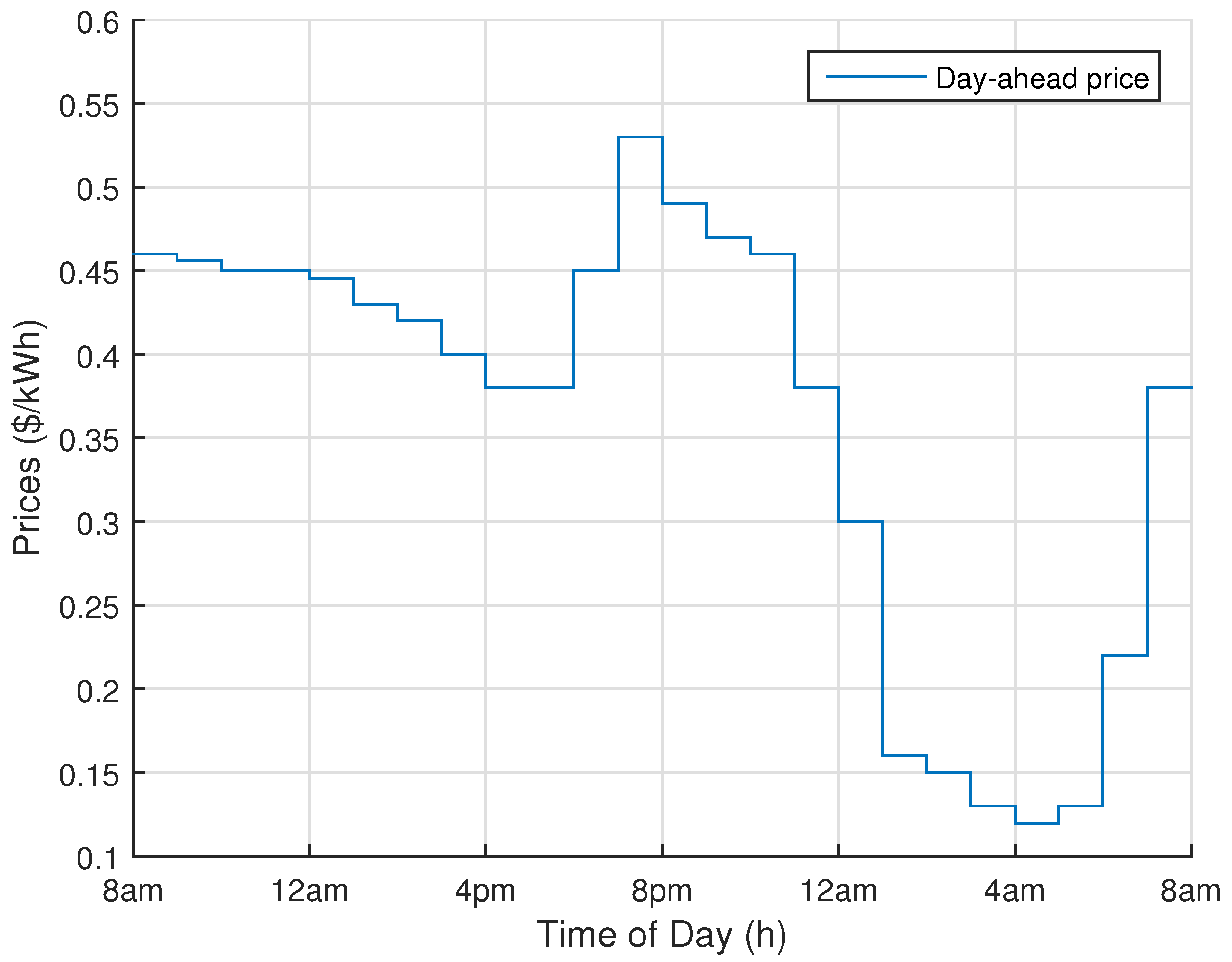
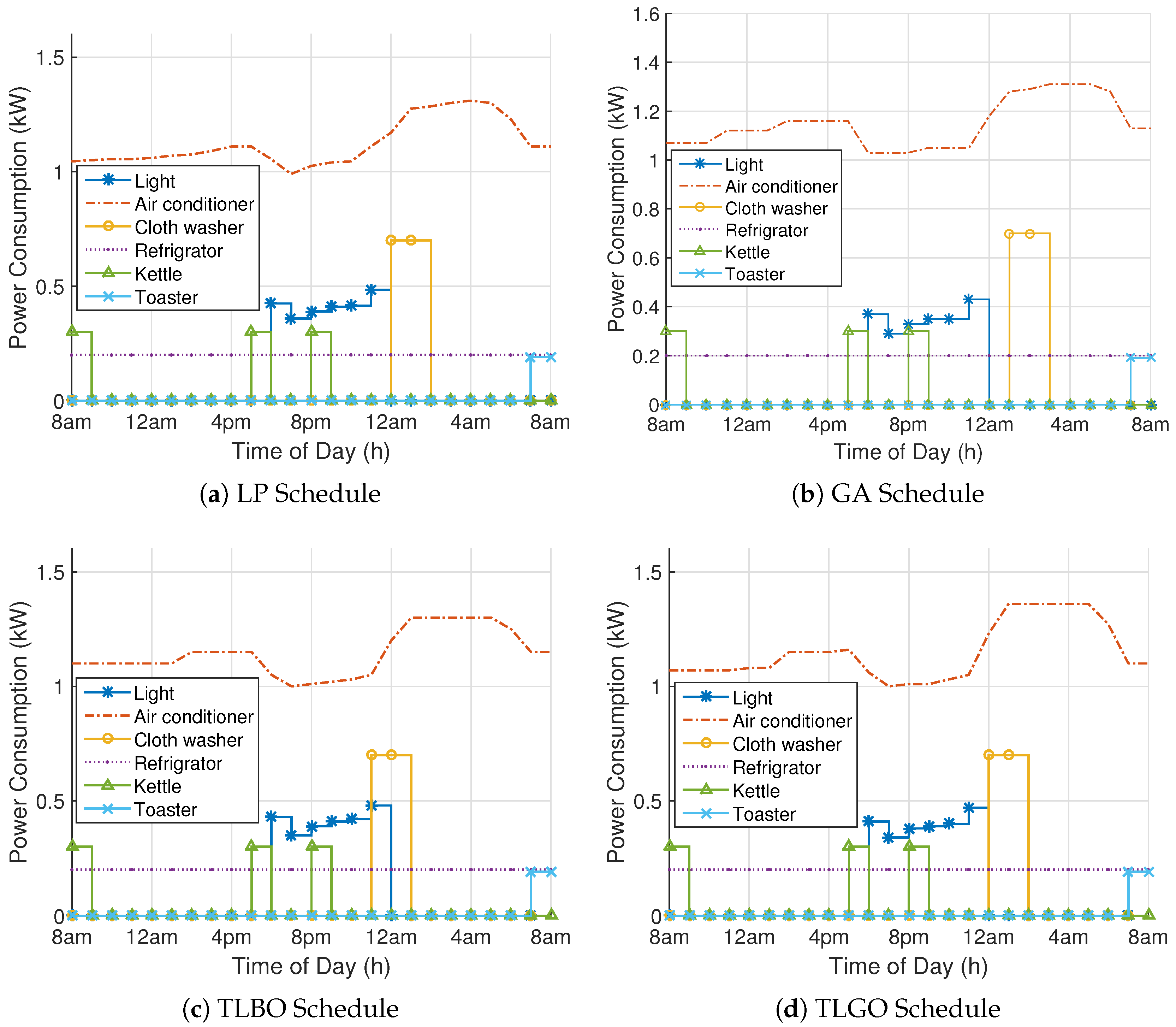
In this section, simulation results and performance of the proposed scheduling technique is discussed in detail. Load scheduling is performed under DAP (shown in Figure 2) and CPP, DAP is taken from the daily report of federal energy regulation commission (FERC) [55]. Total time horizon is 24 h, whereas time slots of 1 h and 15 min are taken for scheduling of appliances. We formulated the problem as an optimization problem with an objective to minimize electricity consumption cost and user discomfort. The problem is solved using three existing optimization techniques: LP, GA, TLBO. We also proposed a hybrid TLGO technique by combining the characteristics of GA and TLBO in order to achieve our objectives. Scheduling results of LP, GA, TLBO and TLGO are provided in Figure 3a–d . Results show that power-flexible appliances operate at low power where prices are high, while time-flexible appliances delay their operation onto off-peak hours. A comparison of all heuristic techniques with LP is shown in Table 4, whereas comparison with state-of-the-art work is provided in Table 5 for 1 h time slot under DAP. A detailed discussion of performance parameters is provided as follows:
7.1. Peak Power Consumption under DAP
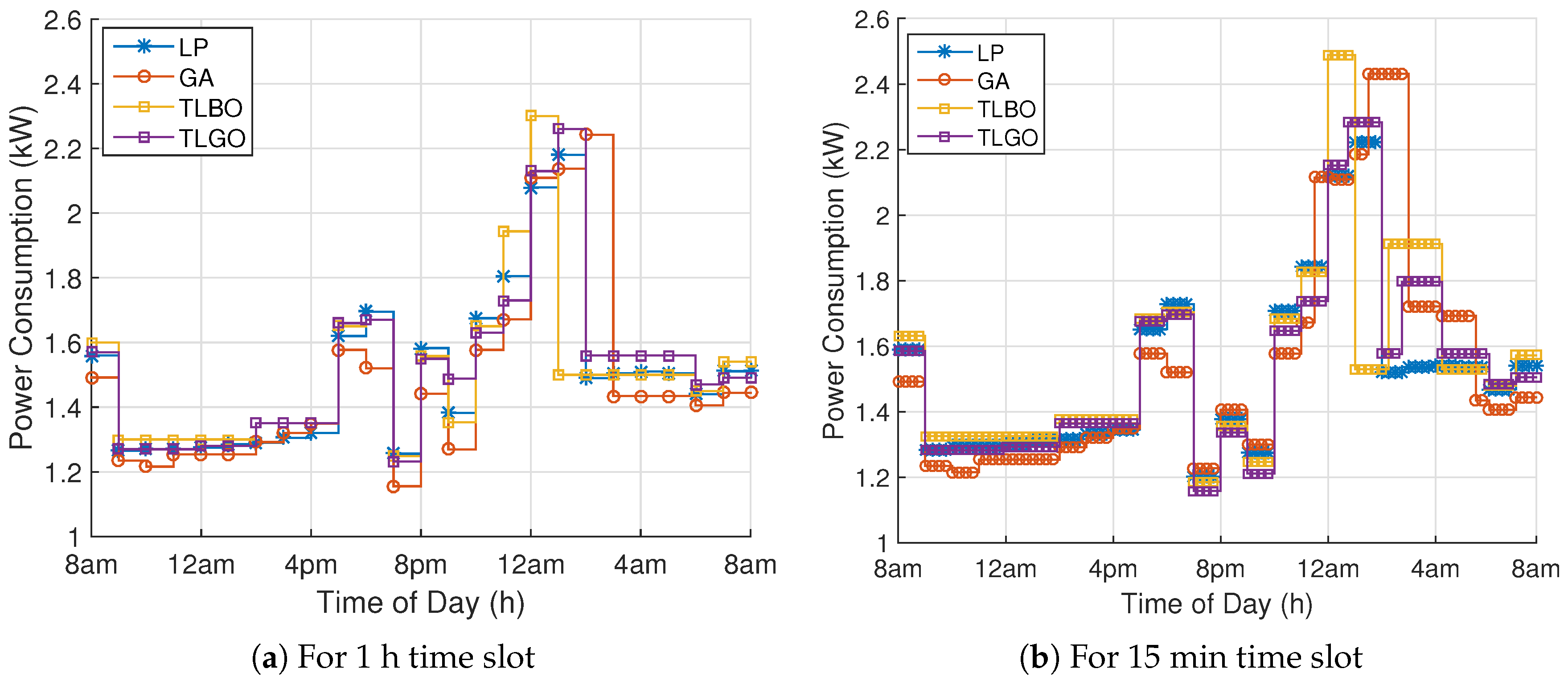
Power consumption depends upon power rating and length of operation time of appliances. Minimizing power consumption during on-peak hours results in minimum cost, however it affects the user discomfort. The power consumption of all appliances for 1 h time slots using LP, GA, TLBO and TLGO is shown in Figure 4a, whereas power consumption for 15 min time slots is provided in Figure 4b. Figure 2 illustrates that 7:00 p.m. to 11:00 p.m. are on-peak hours, whereas 1:00 a.m. to 6:00 am are off-peak hours. So, as to achieve our objectives, power consumption must be minimized in on-peak hours. It can be seen that LP, GA and TLBO has peak power consumption of 2.19 kW, 2.10 kW and 2.42 kW, respectively for 1 h time slot. TLGO has peak hourly power consumption of 2.24 kW, showing that peak power consumption is compromised as compared to LP and GA, however, this can be compensated by minimizing cost and user discomfort as illustrated in Figures 6a and 9a. Peak power consumption of LP, GA, TLBO and TLGO for 15 min time slot is 2.21 kW, 2.41 kW, 2.46 kW and 2.3 kW, respectively. It is evident from the schedule that TLBO has the highest peak power consumption for both, 1 h and 15 min time slot. Results also demonstrate that all the techniques have minimized power consumption during on-peak hours in order to minimize electricity consumption cost. Results also demonstrate that TLGO has best response to time varying prices.
7.2. Peak Power Consumption under CPP
For CPP, we considered the same DAP signal as provided in Figure 2 , with CPP occurring at 7:00 p.m. to 10:00 p.m. During critical peaks, the price for electricity during these time periods is substantially raised [56]. The price during CPP event is doubled as compared to normal prices. The power consumption of all appliances for 1 h time slots using LP, GA, TLBO and TLGO is shown in Figure 5a, whereas power consumption for 15 min time slots is provided in Figure 5b. As 7:00 p.m. to 10:00 p.m. are critical-peak hours, power consumption must be minimized during these periods. For 1 h time slot, LP, GA, TLBO and TLGO has peak power consumption of 2.19 kW, 2.25 kW, 2.32 kW and 2.26 kW, respectively. Similarly, peak power consumption of LP, GA, TLBO and TLGO for 15 min time slot is 2.2 1 kW, 2.41 kW, 2.5 kW and 2.28 kW, respectively.
7.3. Electricity Consumption Cost under DAP
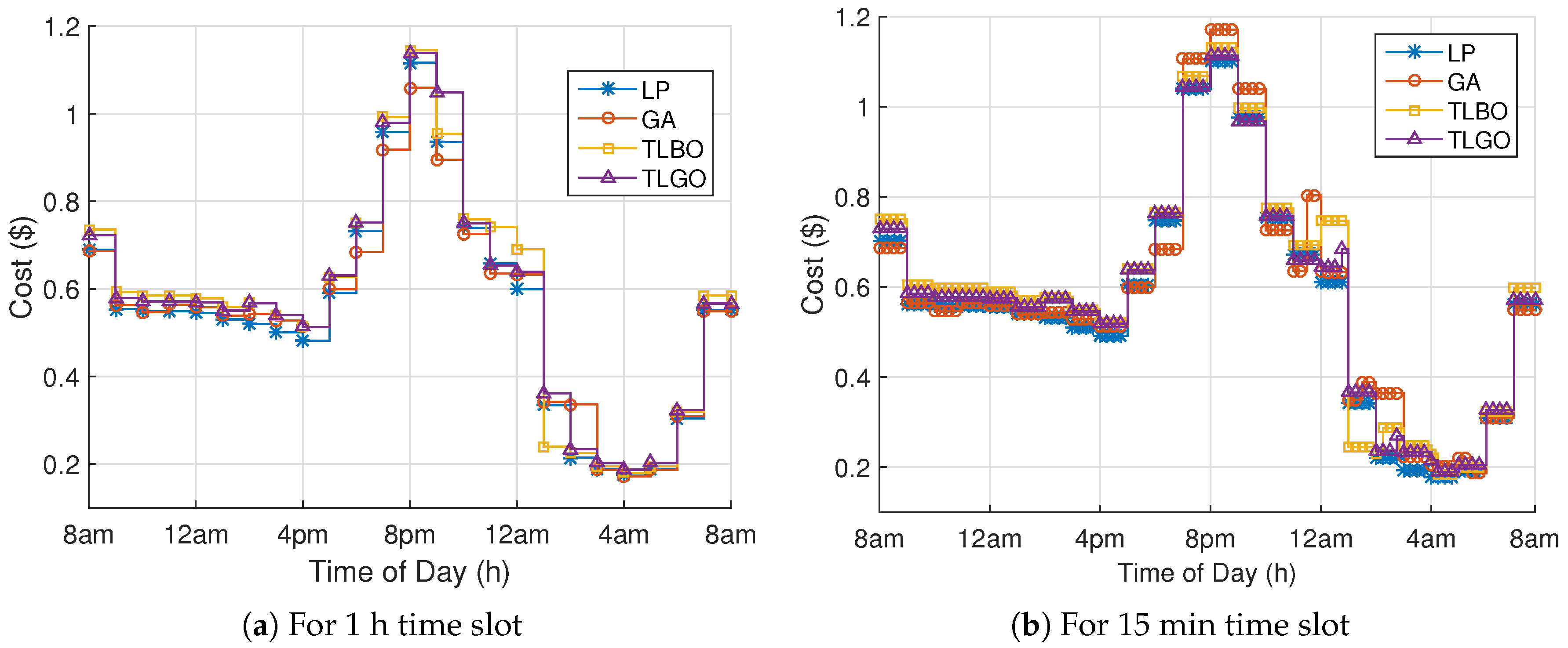
Cost minimization is one of the primary objectives of power scheduling. The aim of scheduling is to minimize consumer’s electricity bill at minimum user discomfort. Consumers participate in load scheduling by consuming more electricity in low peak hours in order to minimize their electricity bill. Daily electricity cost of all the optimization techniques for 1 h time slot is depicted in Figure 6a on hourly basis. The scheduling results for 1 h time slot depicted in Figure 4a shows that all the techniques have scheduled power-flexible appliances at lower power rate where electricity prices are high. Results demonstrate that total daily cost in case of LP is $13.18, whereas GA, TLBO and TLGO have the daily cost of $13.82, $13.70 and $13.37 per day, respectively. Scheduling results of LP, TLBO and TLGO shows nearly similar results for power-flexible appliances. Results for 15 min time slot are given in Figure 6b, showing lower power consumption during period of CPP event. LP, GA, TLBO and TLGO has total cost of $12.97, $13.51,$13.35 and $13.02, respectively, showing that there is no significant effect on cost by increasing the number of time slots (considering smaller time slots), however computational complexity is increased by four time by increase in number of chromosomes and its length. Results also validate that our proposed TLGO algorithm performs well in terms of daily cost reduction. TLGO has the characteristics of both TLBO and GA and is able to maintain a balance between exploitation and exploration mode. So, it performs well in achieving the desired objective.
7.4. Electricity Consumption Cost under CPP
Figure 7a shows the power consumption cost for 1 h time slots by applying LP, GA, TLBO and TLGO. Despite of the fact that power consumption is reduced in case of CPP, results shows that total consumption cost is increased as compared to DAP. The reason for increase in cost is due to high prices during CPP event. Results for 1 h time slots is depicted in Figure 7a, showing high cost during peak periods. Total cost for 1 h time slot by applying LP, GA, TLBO and TLGO is $14.05, $15.22, $14.98 and $14.43, respectively. In case of 15 min time slot (Figure 7b), LP shows the total cost of $13.93, whereas GA, TLBO and TLGO shows the total cost of $14.86, $14.59 and $14.13, respectively.
7.5. Discomfort under DAP
Discomfort minimization is also one of the key aspects of scheduling. User discomfort must be considered along with consumers’ electricity bill minimization to keep consumers motivated for participating in DR. As discussed earlier in Section 4, the two reasons causing user discomfort are: delaying the operation of time-flexible appliances and compressing the power demand of power-flexible appliances. The values of parameters for calculating user discomfort are provided in Table 6. Hourly discomfort caused by power-flexible appliances is illustrated in Figure 8. DAP signal illustrated in Figure 2 shows that 6:00 p.m. to 11:00 p.m. are on-peak hours, so power is compressed, which resulted in user discomfort. For 1 h time slot, overall daily discomfort caused by both types of appliances is depicted in Figure 9a. GA has highest user discomfort of 2.37, whereas discomfort caused by LP, TLBO an TLGO is 1.76, 2.14 and 1.83 respectively. Total discomfort caused by both types of appliances is demonstrated in Figure 9b, showing that LP, GA, TLBO, and TLGO have total discomfort of 2.72, 2.24, 2.08 and 1.78, respectively. Results validate that our proposed TLGO technique performs well in terms of minimizing user discomfort and is able to achieve comparable results with LP by utilizing power in an efficient way.
7.6. Discomfort under CPP
As mentioned earlier Section 7.2, 6:00 p.m. to 10:00 p.m. are critical peak period, and prices are relatively high during these periods. So, power consumption must be minimized in these hours in order to save cost, however this results in user discomfort. For 1 h time slot, overall daily discomfort caused by both types of appliances is depicted in Figure 10a. GA has highest user discomfort of 2.56, whereas discomfort caused by LP and TLBO is 2.32 and 2.52, respectively. Total discomfort caused by both types of appliances in case of 15 min time slot is demonstrated in Figure 10b. Discomfort in case of LP, GA, TLBO and TLGO under CPP is 2.12, 2.46, 2.38 and 2.21, respectively. Results of TLGO and LP are comparable, showing effectiveness of our purposed technique.
7.7. PAR
PAR provides a measure on how peak electricity consumption affects the system, particularly in efficiency and reliability. It shows the power consumption behaviour of consumers and directly effects the operation of peak power plants. So, minimizing PAR is beneficial to both utility and consumer. It benefits utility by maintaining a balance between demand and supply, and consumers by minimize their bill. Minimizing PAR is one of the major objectives of DSM which helps in maintaining the stability and reliability of the power grid. PAR defines the ratio of peak power consumption with the average of total power consumed over the scheduling horizon i.e., from to . The expression for calculating PAR is given as follows,
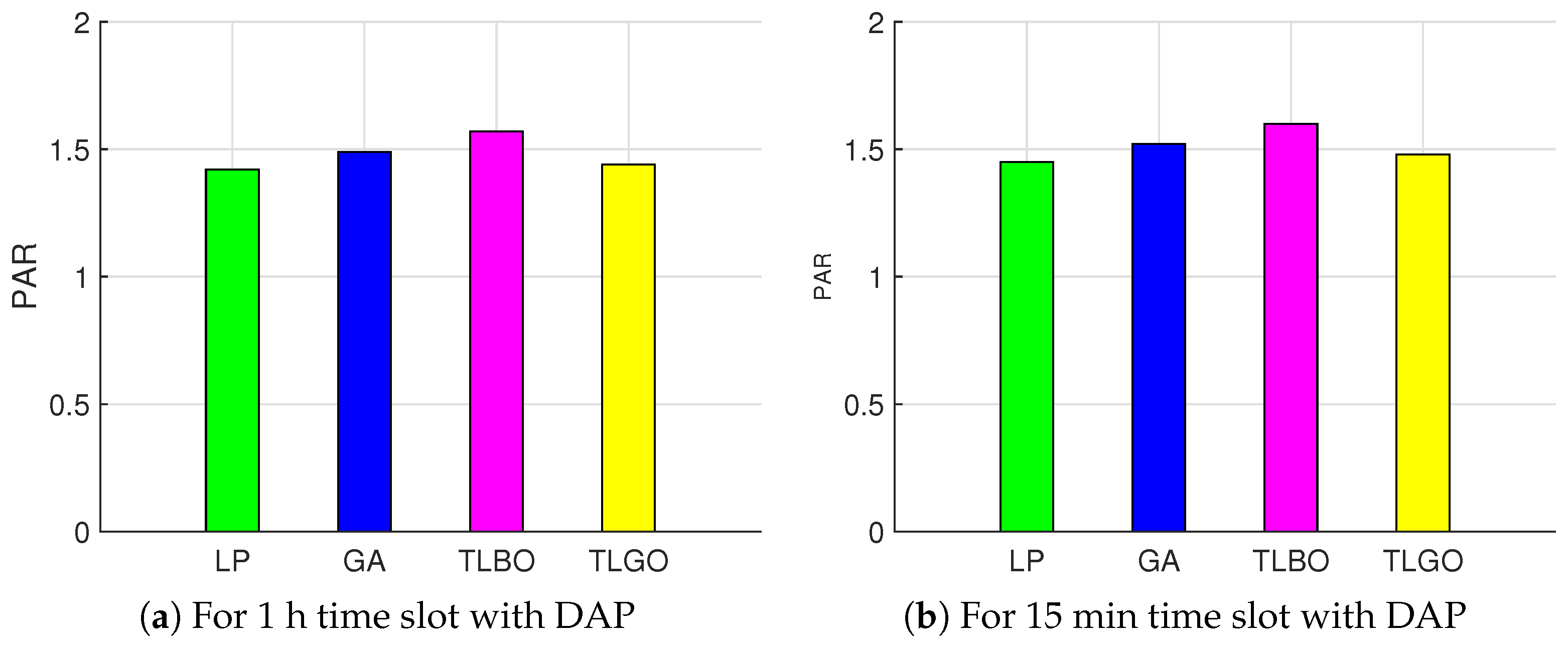
Simulation results of 1 h time slot for PAR are depicted in Figure 11a. TLBO has PAR of 1.57 whereas GA, LP, and TLGO has PAR of 1.49, 1.42 and 1.44, respectively. High PAR in case of TLBO is resulted from peak power consumption (see Figure 4a). Figure 11b shows PAR in case of DAP, whereas Figure 11c,d demonstrates the PAR for 1 h and 15 min time slots, respectively, by implementing CPP scheme. It can be seen clearly from the results that TLGO performs better in terms of minimizing PAR, showing comparable results with LP.
7.8. Feasible Region
A region bounded by the set of points, containing all possible solutions is called feasible region. In our case, electricity consumption cost depends on two factors: the amount of power consumed and electricity price announced by the utility at any particular time slot. As consumers have no control over electricity price, they can only adjust their power consumption pattern in order to minimize cost. There is also a relationship between user discomfort and electricity consumption cost. Minimizing user discomfort results in increased cost.
7.8.1. Feasible Region for Power Consumption and Cost
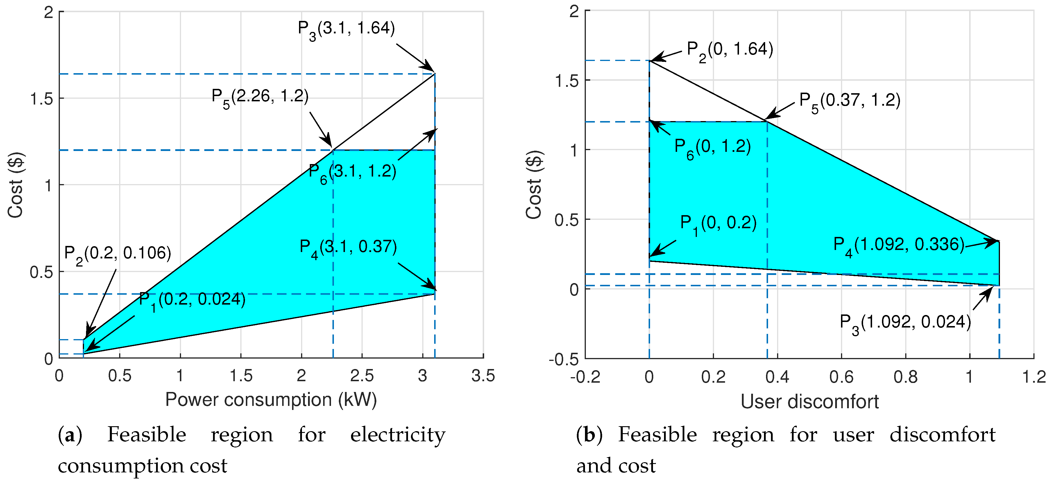
Feasible region for electricity consumption cost under DAP with 1 h time slot is shown in Figure 12a. A region enclosed by points P(0.2, 0.024), P(0.2, 0.106), P(3.1, 0.37), P(2.26, 1.2) and P(3.1, 1.2), represents feasible region for electricity consumption cost. The maximum electricity consumption cost at any specific time slot must not exceed $1.2. P(0.2, 0.024) represents the electricity consumption cost when the minimum allowable load is operating during minimum price slot, whereas P(0.2, 0.106) represents minimum allowable load operating during peak price hour. Moreover, P(3.1, 1.64) and P(3.1, 0.37) represents the minimum and maximum cost when maximum load is being operated during minimum and maximum price hours respectively. P(3.1, 1.64) is excluded from the feasible region after applying cost limit. P(2.26, 1.2) shows the cost of $1.2 at the maximum power consumption of 3.1 kW. P(3.1, 1.2) denotes the cost of $1.2 at the power consumption of 3.1 kW. The line connecting P and P shows that consumers can minimize their electricity consumption cost by consuming more energy during off-peak hours. Similarly, P and P show the same cost at varying power consumption which shows that consumer can utilize maximum power at low cost by modifying his power consumption pattern.
7.8.2. Feasible Region for User Discomfort and Cost
There is an inverse relationship between user discomfort and consumers’ electricity bill. Decreasing user discomfort increases electricity consumption cost and vice versa. Feasible region of user discomfort and cost under DAP with 1 h time slot is illustrated in Figure 12b. P(0, 0.2) represents minimum electricity consumption cost where user discomfort is zero. Similarly, P(0,1.64) shows maximum user discomfort during peak price hours without any user discomfort. is excluded from feasible region by applying the maximum cost limit. Moreover, P(1.092, 0.024) denotes the cost in off-peak hours at user discomfort of 1.092. Similarly, P(1.092, 0.336) represents cost during on-peak hours at maximum user discomfort. P depicts the maximum cost limit of $1.2. The line connecting P and P reflects the same cost at different discomfort levels. This demonstrates that power-flexible appliances can save reasonable cost by compressing their power demand during on-peak hours without compromising the user discomfort.
7.9. Performance Trade-Off
Results show a trade-off between user discomfort and electricity consumption cost. Feasible region for electricity consumption cost illustrated in Figure 12a shows that higher saving can be achieved by scheduling maximum load during off-peak hours. A relationship between user discomfort and cost is illustrated by feasible region depicted in Figure 12b. User discomfort greatly affects electricity consumption cost, as minimizing user discomfort causes an increase in cost and vice versa. Table 7 shows performance tradeoff between cost and user discomfort. GA performs better in terms of minimizing cost, however, user discomfort is very high. User comfort is significantly reduced by applying TLBO, however, peak power demand is very high. Comparison provided in Table 5 shows that TLGO is able to achieve optimal results near to the results of LP. Results also show that TLGO technique performs best is terms of achieving minimal cost and user discomfort.
8. Conclusions
In this paper, a hybrid TLGO algorithm is proposed to minimize electricity consumption cost while minimizing user discomfort. Proposed technique is analyzed for four different performance parameters and compared its performance with LP, GA, and TLBO. Our proposed TLGO algorithm shows the comparable results with LP with less computational efforts. Unlike GA and TLBO, proposed technique minimizes both user discomfort and cost without affecting PAR and peak power consumption. Furthermore, the effect of scheduling on cost and user discomfort is also demonstrated by feasible region. It is also shown that power-flexible appliances have a significant effect on consumers’ electricity bill. Results validate that the proposed TLGO algorithm optimally schedule the load to achieve the desired trade-off between electricity consumption cost and user discomfort.
Acknowledgments
This project was full financially supported by the King Saud University, through the Vice Deanship of Research Chairs.
Author Contributions
Awais Manzoor, Nadeem Javaid, and Ibrar Ullah proposed, implemented, and wrote the optimization schemes. Wadood Abdul, Ahmad Almogren, and Atif Alamri wrote technical sections of the manuscript. All authors refined the manuscript and responded to the queries of the respected reviewers. This was a great team work and all authors jointly accomplished it.
Conflicts of Interest
The authors declare no conflict of interest.
References
- Gungor, C.V.; Sahin, D.; Kocak, T.; Ergut, S.; Buccella, C.; Cecati, C.; Hancke, G.P. Smart grid technologies: Communication technologies and standards. IEEE Trans. Ind. Inform. 2011, 7, 529–539. [Google Scholar] [CrossRef]
- Esther, B.P.; Kumar, K.S. A survey on residential demand side management architecture, approaches, optimization models and methods. Renew. Sustain. Energy Rev. 2016, 59, 342–351. [Google Scholar] [CrossRef]
- Wu, Z.; Tazvinga, H.; Xia, X. Demand side management of photovoltaic-battery hybrid system. Appl. Energy 2015, 148, 294–304. [Google Scholar] [CrossRef]
- Ogunjuyigbe, A.S.O.; Ayodele, T.R.; Oladimeji, O.E. Management of loads in residential buildings installed with PV system under intermittent solar irradiation using mixed integer linear programming. Energy Build. 2016, 130, 253–271. [Google Scholar] [CrossRef]
- El-Baz, W.; Tzscheutschler, P. Short-term smart learning electrical load prediction algorithm for home energy management systems. Appl. Energy 2015, 147, 10–19. [Google Scholar] [CrossRef]
- Sarker, M.R.; Ortega-Vazquez, M.A.; Kirschen, D.S. Optimal coordination and scheduling of demand response via monetary incentives. IEEE Trans. Smart Grid 2015, 6, 1341–1352. [Google Scholar] [CrossRef]
- Erdinc, O.; Paterakis, N.G.; Mendes, T.D.P.; Bakirtzis, A.G.; Catalão, J.P.S. Smart household operation considering bi-directional EV and ESS utilization by real-time pricing-based DR. IEEE Trans. Smart Grid 2015, 6, 1281–1291. [Google Scholar] [CrossRef]
- Bradac, Z.; Kaczmarczyk, V.; Fiedler, P. Optimal scheduling of domestic appliances via MILP. Energies 2014, 8, 217–232. [Google Scholar] [CrossRef]
- Zhang, D.; Shah, N.; Papageorgiou, L.G. Efficient energy consumption and operation management in a smart building with microgrid. Energy Convers. Manag. 2013, 74, 209–222. [Google Scholar] [CrossRef]
- De Angelis, F.; Boaro, M.; Fuselli, D.; Squartini, S.; Piazza, F.; Wei, Q. Optimal home energy management under dynamic electrical and thermal constraints. IEEE Trans. Ind. Inform. 2013, 9, 1518–1527. [Google Scholar] [CrossRef]
- Agnetis, A.; de Pascale, G.; Detti, P.; Vici, A. Load scheduling for household energy consumption optimization. IEEE Trans. Smart Grid 2013, 4, 2364–2373. [Google Scholar] [CrossRef]
- Yu, M.; Hong, S.H. A real-time demand-response algorithm for smart grids: A stackelberg game approach. IEEE Trans. Smart Grid 2016, 7, 879–888. [Google Scholar] [CrossRef]
- Paterakis, N.G.; Erdinc, O.; Bakirtzis, A.G.; Catalão, J.P.S. Optimal household appliances scheduling under day-ahead pricing and load-shaping demand response strategies. IEEE Trans. Ind. Inform. 2015, 11, 1509–1519. [Google Scholar] [CrossRef]
- Marzband, M.; Yousefnejad, E.; Sumper, A.; Domínguez-García, J.L. Real time experimental implementation of optimum energy management system in standalone microgrid by using multi-layer ant colony optimization. Int. J. Electr. Power Energy Syst. 2016, 75, 265–274. [Google Scholar] [CrossRef] [Green Version]
- Belhaiza, S.; Baroudi, U. A game theoretic model for smart grids demand management. IEEE Trans. Smart Grid 2015, 6, 1386–1393. [Google Scholar] [CrossRef]
- Reka, S.S.; Ramesh, V. A demand response modeling for residential consumers in smart grid environment using game theory based energy scheduling algorithm. Ain Shams Eng. J. 2016, 7, 835–845. [Google Scholar] [CrossRef]
- Soares, A.; Gomes, A.; Antunes, C.H.; Oliveira, C. A Customized Evolutionary Algorithm for Multi-Objective Management of Residential Energy Resources. IEEE Trans. Ind. Inform. 2017, 13, 492–501. [Google Scholar] [CrossRef]
- Yi, P.; Dong, X.; Iwayemi, A.; Zhou, C.; Li, S. Real-time opportunistic scheduling for residential demand response. IEEE Trans. Smart Grid 2013, 4, 227–234. [Google Scholar] [CrossRef]
- Rastegar, M.; Fotuhi-Firuzabad, M.; Zareipour, H. Home energy management incorporating operational priority of appliances. Int. J. Electr. Power Energy Syst. 2016, 74, 286–292. [Google Scholar] [CrossRef]
- Wang, J.; Li, Y.; Zhou, Y. Interval number optimization for household load scheduling with uncertainty. Energy Build. 2016, 130, 613–624. [Google Scholar] [CrossRef]
- Shirazi, E.; Jadid, S. Optimal residential appliance scheduling under dynamic pricing scheme via HEMDAS. Energy Build. 2015, 93, 40–49. [Google Scholar] [CrossRef]
- Althaher, S.; Mancarella, P.; Mutale, J. Automated demand response from home energy management system under dynamic pricing and power and comfort constraints. IEEE Trans. Smart Grid 2015, 6, 1874–1883. [Google Scholar] [CrossRef]
- Samadi, P.; Wong, V.W.S.; Schober, R. Load scheduling and power trading in systems with high penetration of renewable energy resources. IEEE Trans. Smart Grid 2016, 7, 1802–1812. [Google Scholar] [CrossRef]
- Tan, Z.; Yang, P.; Nehorai, A. An optimal and distributed demand response strategy with electric vehicles in the smart grid. IEEE Trans. Smart Grid 2014, 5, 861–869. [Google Scholar] [CrossRef]
- Chakraborty, S.; Ito, T.; Senjyu, T.; Saber, A.Y. Intelligent economic operation of smart-grid facilitating fuzzy advanced quantum evolutionary method. IEEE Trans. Sustain. Energy 2013, 4, 905–916. [Google Scholar] [CrossRef]
- Rajalingam, S.; Malathi, V. HEM algorithm based smart controller for home power management system. Energy Build. 2016, 131, 184–192. [Google Scholar]
- Muralitharan, K.; Sakthivel, R.; Shi, Y. Multiobjective optimization technique for demand side management with load balancing approach in smart grid. Neurocomputing 2016, 177, 110–119. [Google Scholar] [CrossRef]
- Alham, M.H.; Elshahed, M.; Ibrahim, D.K.; El Zahab, E.E.D.A. A dynamic economic emission dispatch considering wind power uncertainty incorporating energy storage system and demand side management. Renew. Energy 2016, 96, 800–811. [Google Scholar] [CrossRef]
- Serra, J.; Pubill, D.; Antonopoulos, A.; Verikoukis, C. Smart HVAC control in IoT: Energy consumption minimization with user comfort constraints. Sci. World J. 2014, 2014, 161874. [Google Scholar] [CrossRef] [PubMed]
- Anvari-Moghaddam, A.; Monsef, H.; Rahimi-Kian, A. Optimal smart home energy management considering energy saving and a comfortable lifestyle. IEEE Trans. Smart Grid 2015, 6, 324–332. [Google Scholar] [CrossRef]
- Pilloni, V.; Floris, A.; Meloni, A.; Atzori, L. Smart Home Energy Management Including Renewable Sources: A QoE-driven Approach. IEEE Trans. Smart Grid 2016. [Google Scholar] [CrossRef]
- Adika, C.O.; Wang, L. Smart charging and appliance scheduling approaches to demand side management. Int. J. Electr. Power Energy Syst. 2014, 57, 232–240. [Google Scholar] [CrossRef]
- Kusakana, K. Energy management of a grid-connected hydrokinetic system under Time of Use tariff. Renew. Energy 2017, 101, 1325–1333. [Google Scholar] [CrossRef]
- Vardakas, J.S.; Zorba, N.; Verikoukis, C.V. Performance evaluation of power demand scheduling scenarios in a smart grid environment. Appl. Energy 2015, 142, 164–178. [Google Scholar] [CrossRef]
- Vardakas, J.S.; Zorba, N.; Verikoukis, C.V. Power demand control scenarios for smart grid applications with finite number of appliances. Appl. Energy 2016, 162, 83–98. [Google Scholar] [CrossRef]
- Bharathi, C.; Rekha, D.; Vijayakumar, V. Genetic Algorithm Based Demand Side Management for Smart Grid. Wirel. Pers. Commun. 2017, 93, 481–502. [Google Scholar] [CrossRef]
- Gupta, A.; Singh, B.P.; Kumar, R. Optimal provision for enhanced consumer satisfaction and energy savings by an intelligent household energy management system. In Proceedings of the 2016 IEEE 6th International Conference on Power Systems (ICPS), New Delhi, India, 4–6 March 2016; pp. 1–6. [Google Scholar]
- Javaid, N.; Ullah, I.; Akbar, M.; Iqbal, Z.; Khan, F.A.; Alrajeh, N.; Alabed, M.S. An Intelligent Load Management System with Renewable Energy Integration for Smart Homes. IEEE Access 2017, 5, 13587–13600. [Google Scholar] [CrossRef]
- Ogunjuyigbe, A.S.O.; Ayodele, T.R.; Akinola, O.A. User satisfaction-induced demand side load management in residential buildings with user budget constraint. Appl. Energy 2017, 187, 352–366. [Google Scholar] [CrossRef]
- Zhu, Z.; Tang, J.; Lambotharan, S.; Chin, W.H.; Fan, Z. An integer linear programming based optimization for home demand-side management in smart grid. In Proceedings of the 2012 IEEE PES In Innovative Smart Grid Technologies (ISGT), Washington, DC, USA, 16–20 January 2012; pp. 1–5. [Google Scholar]
- Ma, J.; Chen, H.H.; Song, L.; Li, Y. Residential load scheduling in smart grid: A cost efficiency perspective. IEEE Trans. Smart Grid 2016, 7, 771–784. [Google Scholar] [CrossRef]
- Li, C.; Yu, X.; Yu, W.; Chen, G.; Wang, J. Efficient computation for sparse load shifting in demand side management. IEEE Trans. Smart Grid 2017, 8, 250–261. [Google Scholar] [CrossRef]
- Bahrami, S.; Sheikhi, A. From demand response in smart grid toward integrated demand response in smart energy hub. IEEE Trans. Smart Grid 2016, 7, 650–658. [Google Scholar] [CrossRef]
- Moon, S.; Lee, J.-W. Multi-Residential Demand Response Scheduling with Multi-Class Appliances in Smart Grid. IEEE Trans. Smart Grid 2016. [Google Scholar] [CrossRef]
- Zhang, D.; Evangelisti, S.; Lettieri, P.; Papageorgiou, L.G. Economic and environmental scheduling of smart homes with microgrid: DER operation and electrical tasks. Energy Convers. Manag. 2016, 110, 113–124. [Google Scholar] [CrossRef]
- Dupont, B.; Tant, J.; Belmans, R. Automated residential demand response based on dynamic pricing. In Proceedings of the 2012 3rd IEEE PES International Conference and Exhibition on Innovative Smart Grid Technologies (ISGT Europe), Berlin, Germany, 14–17 October 2012; pp. 1–7. [Google Scholar]
- Safdarian, A.; Fotuhi-Firuzabad, M.; Lehtonen, M. Optimal residential load management in smart grids: A decentralized framework. IEEE Trans. Smart Grid 2016, 7, 1836–1845. [Google Scholar] [CrossRef]
- Asare-Bediako, B.; Kling, W.L.; Ribeiro, P.F. Integrated agent-based home energy management system for smart grids applications. In Proceedings of the 2013 4th IEEE/PES Innovative Smart Grid Technologies Europe (ISGT EUROPE), Lyngby, Denmark, 6–9 October 2013; pp. 1–5. [Google Scholar]
- Sou, K.C.; Weimer, J.; Sandberg, H.; Johansson, K.H. Scheduling smart home appliances using mixed integer linear programming. In Proceedings of the 2011 50th IEEE Conference on Decision and Control and European Control Conference (CDC-ECC), Orlando, FL, USA, 12–15 December 2011; pp. 5144–5149. [Google Scholar]
- Ma, K.; Yao, T.; Yang, J.; Guan, X. Residential power scheduling for demand response in smart grid. Int. J. Electr. Power Energy Syst. 2016, 78, 320–325. [Google Scholar] [CrossRef]
- Taguchi, G.; Chowdhury, S.; Wu, Y. Taguchi’s Quality Engineering Handbook; John Wiley and Sons: Hoboken, NJ, USA, 2005; p. 1736. [Google Scholar]
- Fadel, E.; Gungor, V.C.; Nassef, L.; Akkari, N.; Malik, M.A.; Almasri, S.; Akyildiz, I.F. A survey on wireless sensor networks for smart grid. Comput. Commun. 2015, 71, 22–33. [Google Scholar] [CrossRef]
- Depuru, S.S.S.R.; Wang, L.; Devabhaktuni, V. Smart meters for power grid: Challenges, issues, advantages and status. Renew. Sustain. Energy Rev. 2011, 15, 2736–2742. [Google Scholar] [CrossRef]
- Rao, R.V.; Savsani, V.J.; Vakharia, D.P. Teaching-learning-based optimization: A novel method for constrained mechanical design optimization problems. Comput. Aided Des. 2011, 43, 303–315. [Google Scholar] [CrossRef]
- Real-Time Pricing for Residential Customers, MISO Daily Report Archives. 2012. Available online: https://ferc.gov/market-oversight/mkt-electric/midwest/miso-archives.asp (accessed on 3 February 2016).
- Time Based Rate Programs, Critical Peak Pricing. Available online: https://www.smartgrid.gov/recovery_act/time_based_rate_programs.html (accessed on 15 April 2017).
Figure 1.
Proposed HEMS architecture.
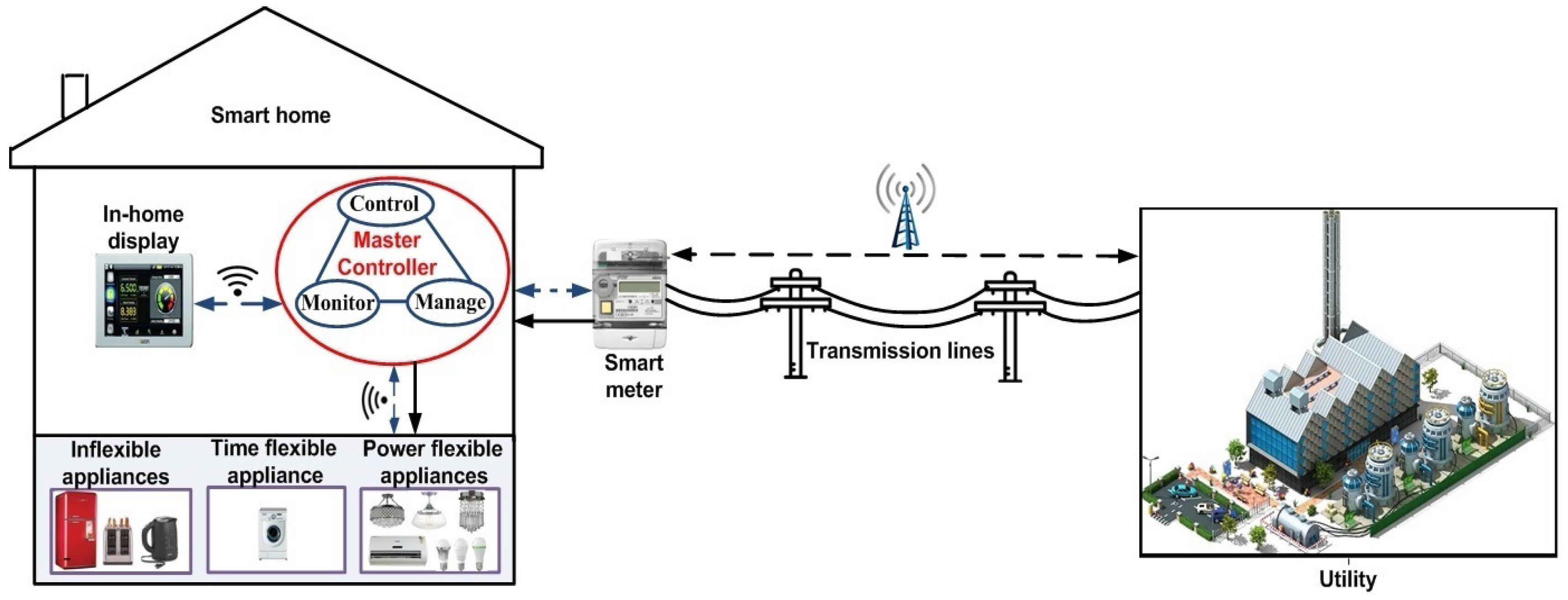
Figure 2.
DAP (Day-Ahead Price) signal.

Figure 3.
Appliances schedule with DAP for 1 h time slot.

Figure 4.
Power consumption of appliances under DAP.
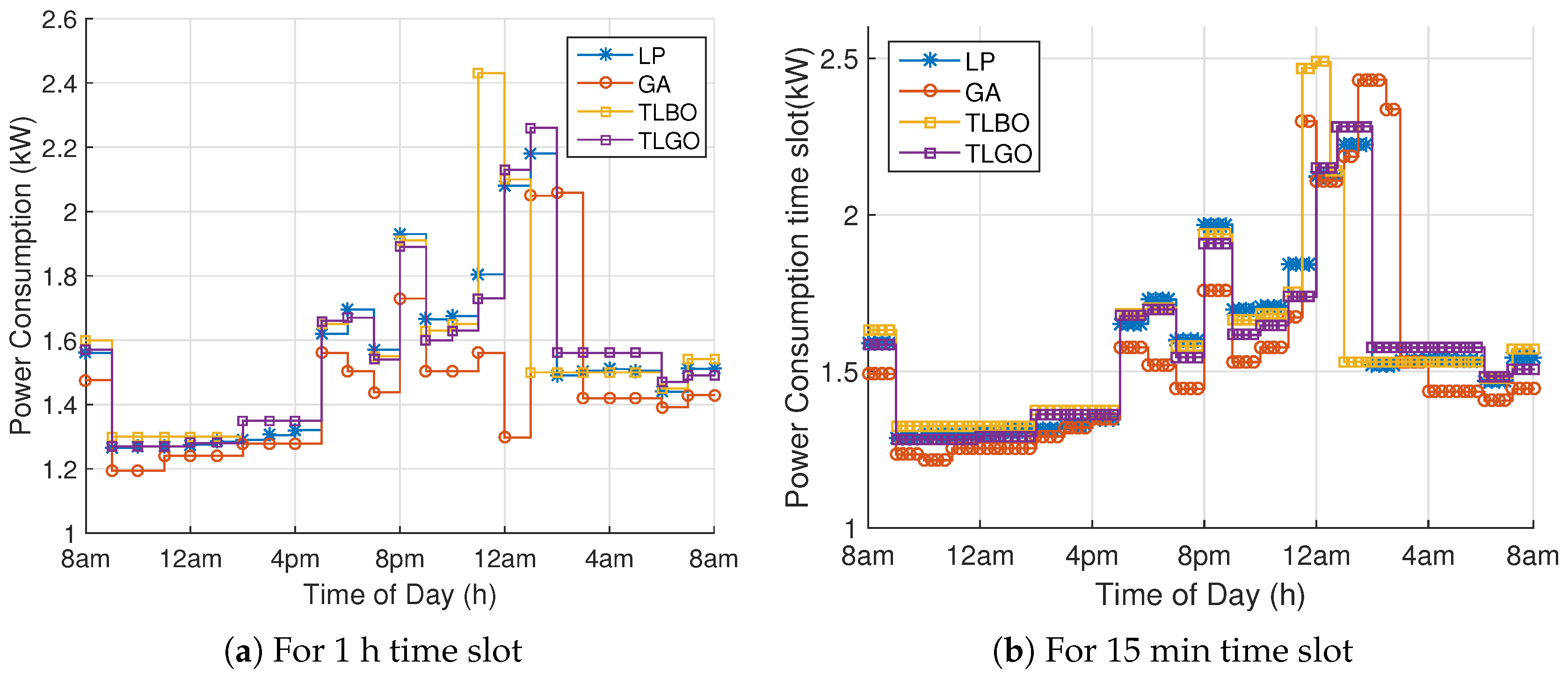
Figure 5.
Power consumption of appliances under CPP.

Figure 6.
Electricity consumption cost under DAP.

Figure 7.
Electricity consumption cost under CPP.

Figure 8.
Hourly discomfort of appliances under DAP (1 h time slot).
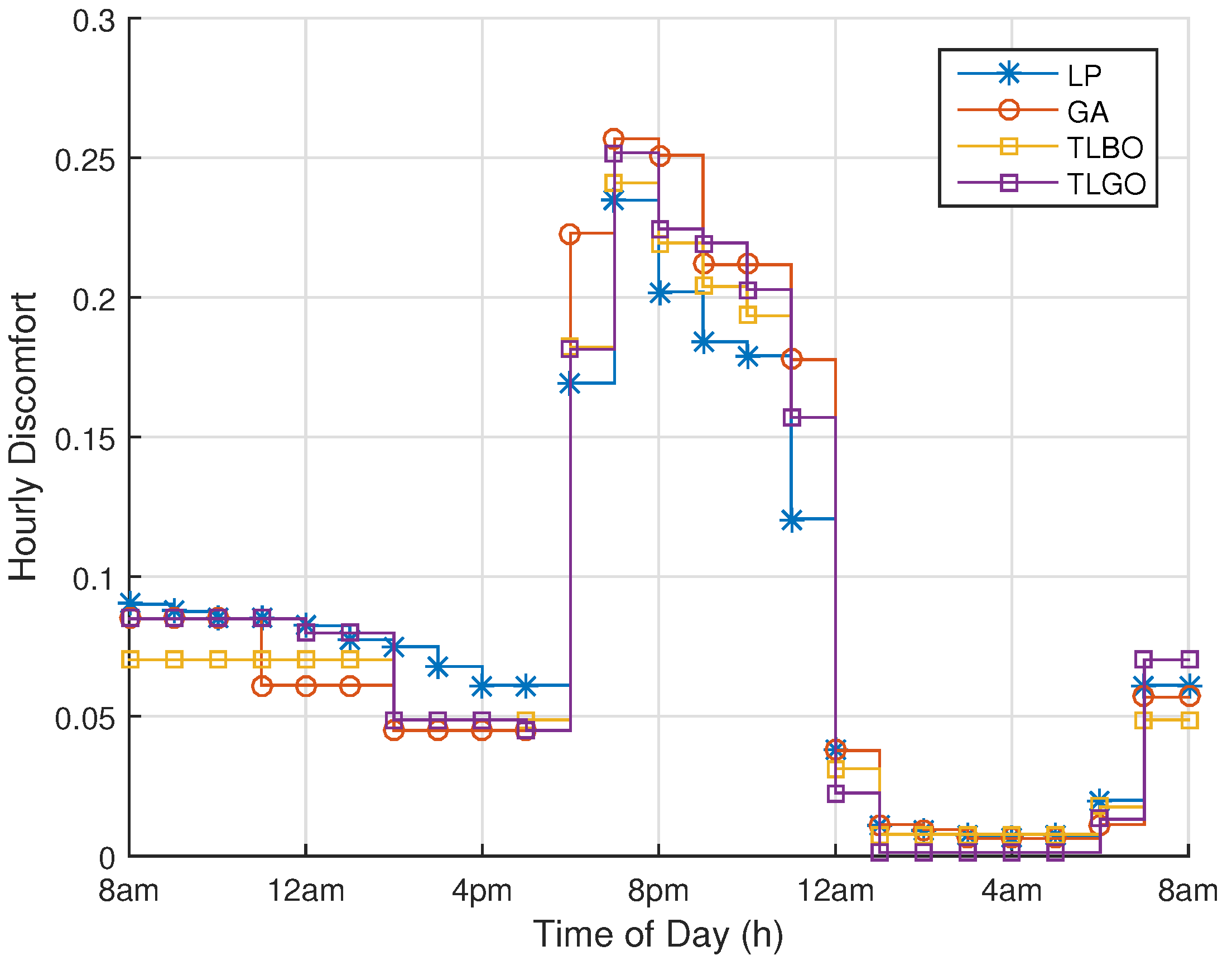
Figure 9.
Discomfort under DAP.
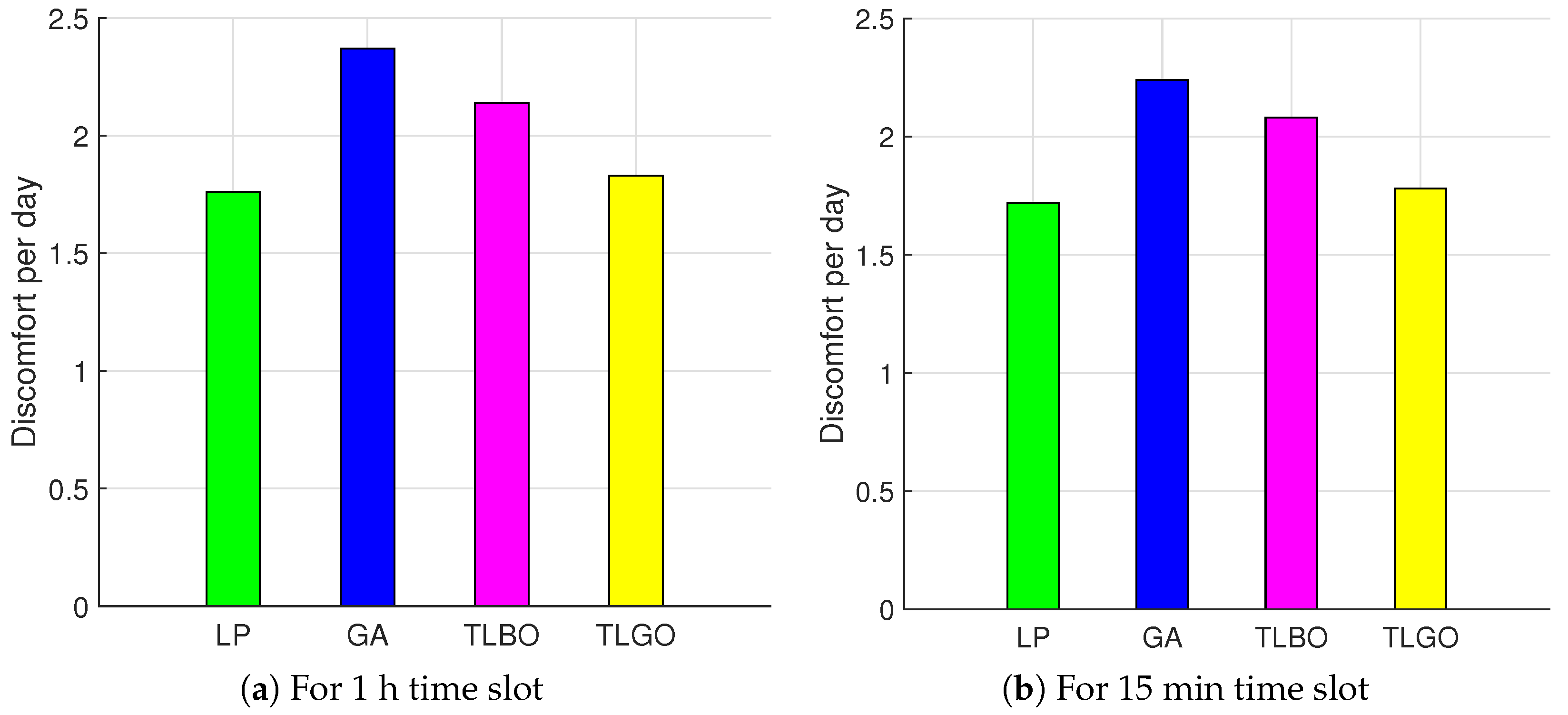
Figure 10.
Discomfort under CPP.
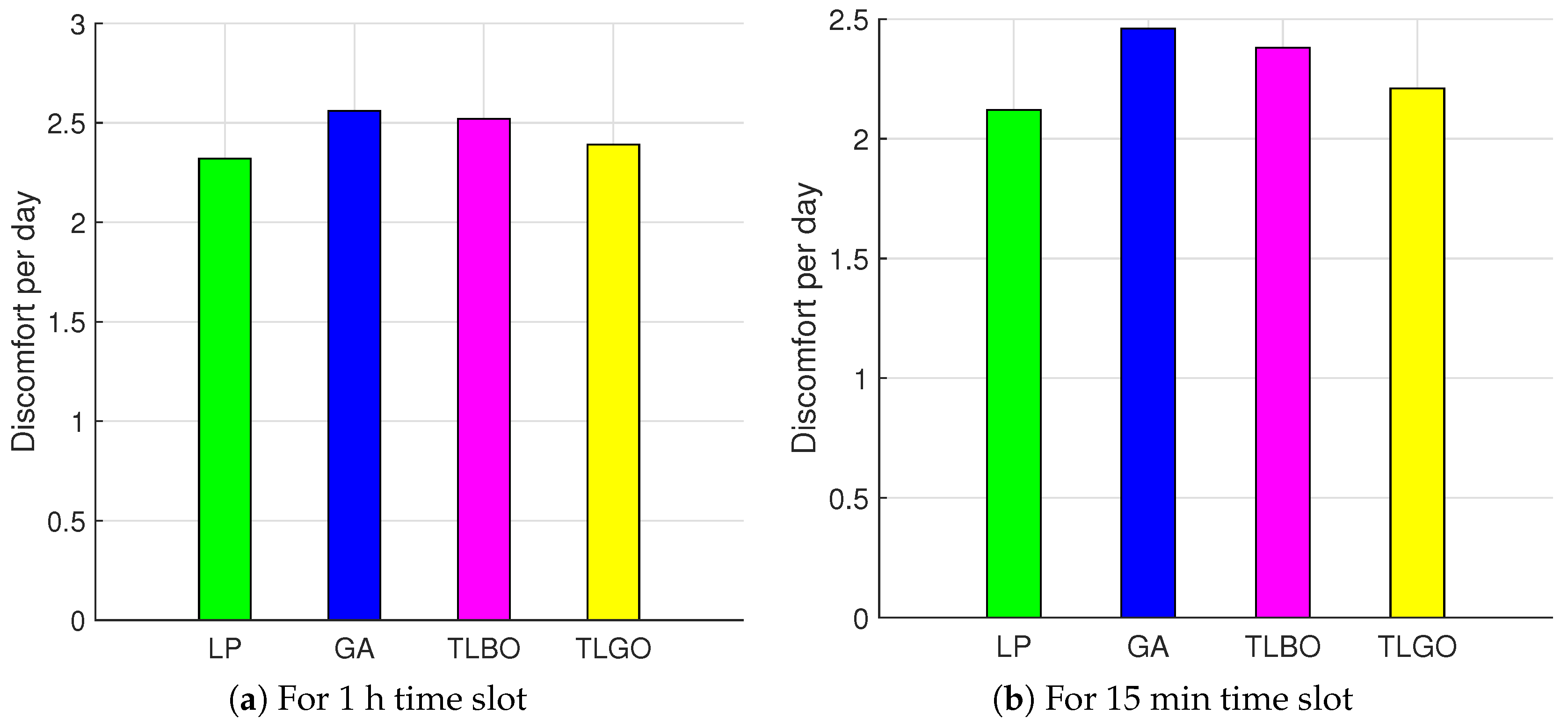
Figure 11.
PAR.

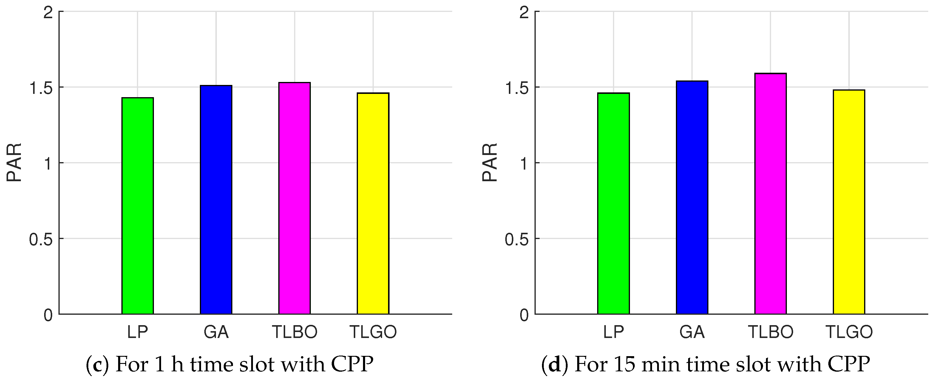
Figure 12.
PAR.

Table 1.
Strength and limitations of state-of-the-art work.
| Technique | Objective | Features | Remarks |
|---|---|---|---|
| BPSO and ILP [20] | Cost minimization and thermal comfort maximization | Interval number analysis to handel uncertain hot water demand and ambient temperature | System complexity |
| MINLP [21] | Minimize cost and maximize user comfort | Considered both thermal and electrical appliances and study seasonal price variations and their effect on cost | PAR is ignored |
| MINLP [22] | Consumers’ bill reduction | High prices are applied to restrict the load below the threshold | High computational complexity |
| Approximate dynamic programming [23] | Maximize revenue generated by RES | Energy trading among consumers | No mechanism to handle uncertainties caused by integration of RES |
| Distributed Optimization algorithm [24] | Minimize consumers’ electricity bill | Integration of RES and PHEV for energy trading | User dissatisfaction |
| Quantum EA [25] | Minimize carbon emissions and production cost | Fuzzy logic is used to handel uncertainties caused by integration of RES | User comfort is compromized |
| HEMS algorithm with source priority [26] | Minimize cost and peak power demand | Maximize the utilization of solar panel and improve the quality of power by selective harmonic elimination method | Uncertainties caused by integration of RES are not considered |
| Multi-objective EA [27] | Minimize cost and waiting time of appliances | Admission control mechanism to manage residential load | Power-flexible appliances are not taken into consideration |
| Branch and bound [28] | Cost and carbon emission reduction | Increase the utilization of wind energy and ESS | User comfort is not handeled |
| LP [32] | Minimize consumers’ electricity bill | Use of aggregator to coordinate the charging and discharging of batteries | PAR and user satisfaction is totally ignored |
| Analytical model [34,35] | Reduce cost and peak power demand | Recursive formulas to determine the distribution of power units in use | Assumption of infinite number of appliances [34] results in overestimation |
| GA [36] | Minimize power consumption in residential, commercial and industrial sector | Performance of proposed model is compared with other evolutionary algorithms | PAR is compromised |
| GA and MILP [37] | Minimization of consumers’ bill | Integration of RES and ESS and a mechanism is presented to sale surplus energy to gird | Consumers’ frustration |
| GA [39] | Minimize cost while maximizing user satisfaction | Manage the load in user defined budget | PAR is ignored |
| ILP [40] | Minimize peak hoyrly load | Increasing number of appliances results in balanced load | Users have little incentives to participate in load scheduling |
| Fractional programming [41] | Consumers’ bill reduction | Proposed a novel concept of cost efficiency | PAR is compromised |
| MILP and Mixed integer quadratic programming [47] | Minimize cost and achieved and balanced load curve | 50 households are taken into consideration | High computational complexity |
| MILP [49] | Consumers’ bill reduction | Different energy phases of appliances are discussed | Inscalable |
Table 2.
Appliances parameter.
| Appliance Name | Class | Power Rating (kW) | Starting Time | Finishing Time | Length of Operation Time |
|---|---|---|---|---|---|
| Cloth washer | Time-flexible | 0.7 | 6:00 p.m. | 7:00 a.m. | 2 h |
| Lights | Power-flexible | 0.2–0.8 | 6:00 p.m. | 11:00 p.m. | 6 h |
| Air conditioner | Power-flexible | 0–1.4 | 8:00 a.m. | 8:00 a.m. | 24 h |
| Kettle | Inflexible | 1.2 | 8:00 a.m., 5:00 p.m., 8:00 p.m. | 9:00 a.m., 6:00 p.m., 9:00 p.m. | 15 min |
| Toaster | Inflexible | 1.2 | 7:00 a.m. | 8:00 a.m. | 10 min |
| Refrigerator | Inflexible | 0.2 | 8:00 a.m. | 8:00 a.m. | 24 h |
Table 3.
GA parameters.
| Parameters | Values |
|---|---|
| Population size | 300 |
| Number of iterations | 200 |
| 0.9 | |
| 0.1 |
Table 4.
Comparison of GA, TLBO and TLGO with LP under DAP for 1 h time slot.
| Technique Name | Daily Cost | Daily Discomfort | Peak Power Consumption | PAR |
|---|---|---|---|---|
| GA | 4.85% increase | 13.89% increase | 1.02% increase | 4.93% increase |
| TLBO | 3.96% increase | 8.73% increase | 10.5% increase | 9.48% increase |
| TLGO | 1.44% increase | 2.98% increase | 2.18% increase | 0.86% increase |
Table 5.
Comparison with literature.
| Ref. | Discomfort | Cost Savings |
|---|---|---|
| Pilloni et al. [31] | 1.65–1.70 (Annoyance rate) | 33% |
| Ogunjuyigbe et al. [39] | 9.6 (Dissatisfaction level) | |
| 20.2 (Dissatisfaction level) | ||
| 30.9 (Dissatisfaction level) | ||
| Y. Peizhong et al. [18] | 7.64 h (Average monthly delay) | 20% |
| K. Muralitharan et al. [27] | 73.32 s average delay (By considering 10 appliances) | 38% |
| 76.28 s average delay (By considering 11 appliances) | ||
| 86.83 s average delay (By considering 12 appliances) | ||
| 94.39 s average delay (By considering 13 appliances) | ||
| 107.58 s average delay (By considering 14 appliances) | ||
| K. Ma et al. [50] | 1.76 | 34% |
| GA (Proposed) | 2.37 | 31% |
| TLBO (Proposed) | 2.14 | 31.5% |
| TLGO (Proposed) | 1.83 | 33% |
Table 6.
Discomfort parameter.
| Appliance | k | ||
|---|---|---|---|
| Cloth washer | 3 | 0.001 | - |
| Lights | - | - | [0.5–1] |
| Air conditioner | - | - | [0.4–1] |
Table 7.
Performance trade-off.
| Discomfort | Cost ($) |
|---|---|
| 0 | 22.00 |
| 2 | 13.42 |
| 2.2 | 13.00 |
| 4 | 11.85 |
© 2017 by the authors. Licensee MDPI, Basel, Switzerland. This article is an open access article distributed under the terms and conditions of the Creative Commons Attribution (CC BY) license (http://creativecommons.org/licenses/by/4.0/).
Share and Cite
MDPI and ACS Style
Manzoor, A.; Javaid, N.; Ullah, I.; Abdul, W.; Almogren, A.; Alamri, A. An Intelligent Hybrid Heuristic Scheme for Smart Metering based Demand Side Management in Smart Homes. Energies 2017, 10, 1258. https://doi.org/10.3390/en10091258
AMA Style
Manzoor A, Javaid N, Ullah I, Abdul W, Almogren A, Alamri A. An Intelligent Hybrid Heuristic Scheme for Smart Metering based Demand Side Management in Smart Homes. Energies. 2017; 10(9):1258. https://doi.org/10.3390/en10091258
Chicago/Turabian StyleManzoor, Awais, Nadeem Javaid, Ibrar Ullah, Wadood Abdul, Ahmad Almogren, and Atif Alamri. 2017. "An Intelligent Hybrid Heuristic Scheme for Smart Metering based Demand Side Management in Smart Homes" Energies 10, no. 9: 1258. https://doi.org/10.3390/en10091258
Note that from the first issue of 2016, this journal uses article numbers instead of page numbers. See further details here.