Game-Based Generation Scheduling Optimization for Power Plants Considering Long-Distance Consumption of Wind-Solar-Thermal Hybrid Systems

Abstract
:1. Introduction
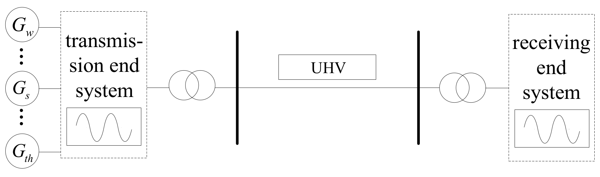
2. System Model
2.1. Generation Cost
2.2. Additional Cost
3. Problem Formulation
3.1. Bids of Power Plants
3.2. Market Clearing Model
- represents the bidding price of power plant m at time slot h;represents the trading generating volume of power plant m at time slot h;
- represents the load demand of the receiving end system at h;
- denotes maximum capacity of the UHV transmission line;
- denotes minimum output of power plant m;
- denote maximum output of power plant m;
- denotes minimum output of thermal power plants;
- denotes maximum output of thermal power plants;
- denotes downward ramp rate of thermal power plants;
- denotes upward ramp rate of thermal power plants.
4. Non-Cooperative Game among Power Plants
- denotes trading price at time slot h in the intraday market;
- denotes generating volume at time slot h in the intraday market;
- denotes the difference between practical generation and cleared generation;
- denotes the installed capacity of power plant;
- denotes the penalty coefficient.
| Algorithm 1: Calculation of the decision-making model |
| Randomly initialize |
| While do |
| Determine power generation dispatch policy by solving problem (Equation (11)). |
| Select optimal bidding parameter in strategies set by using the interior point method. |
| if then |
| end if |
| End while |
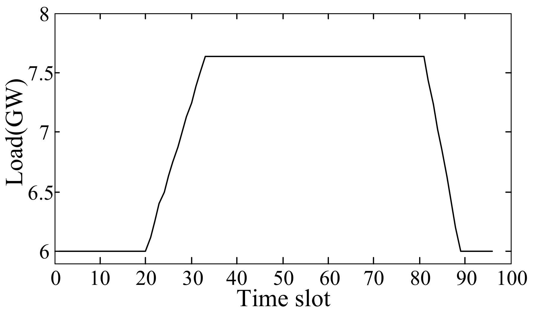
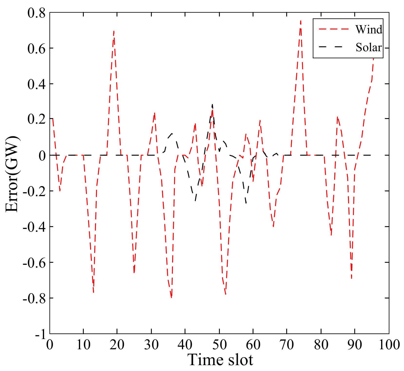
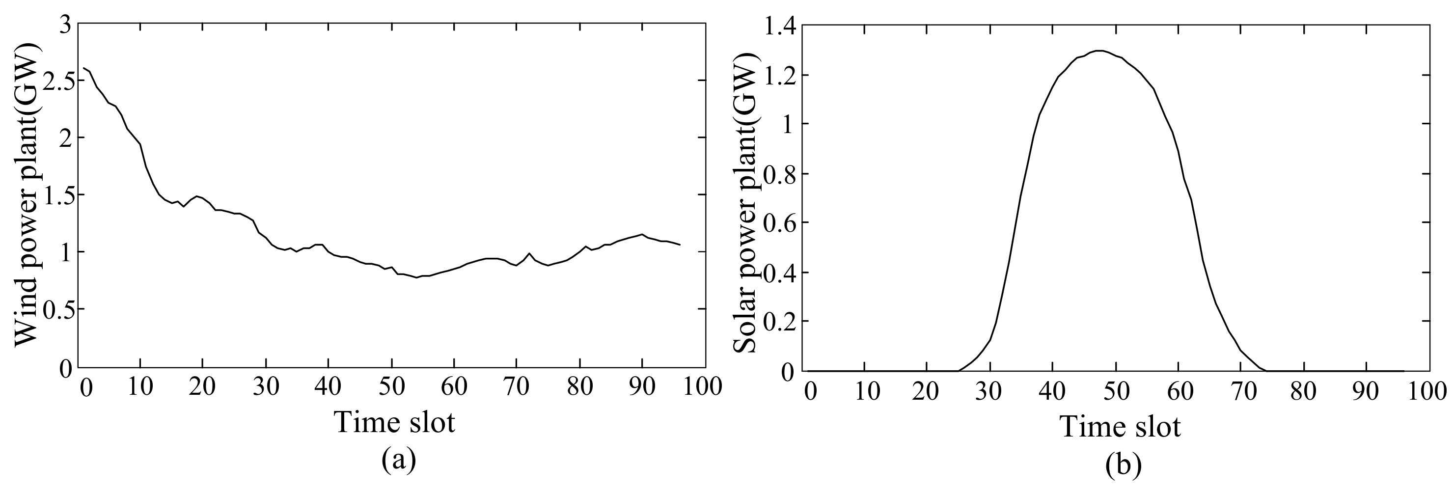
5. Case Study
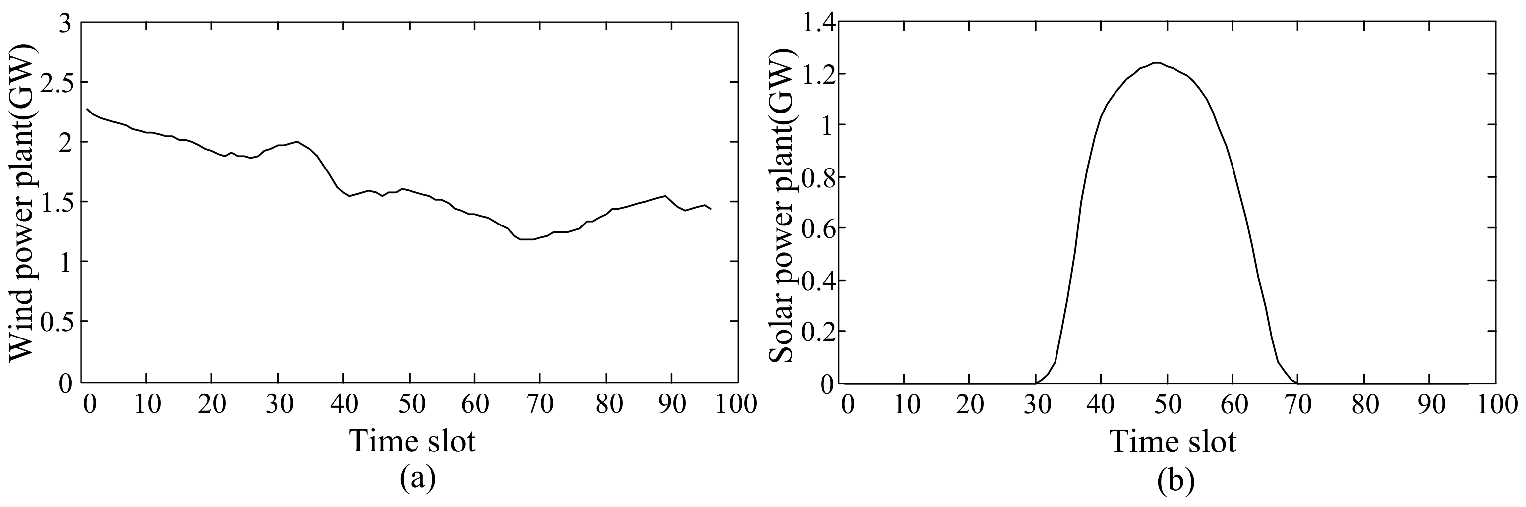
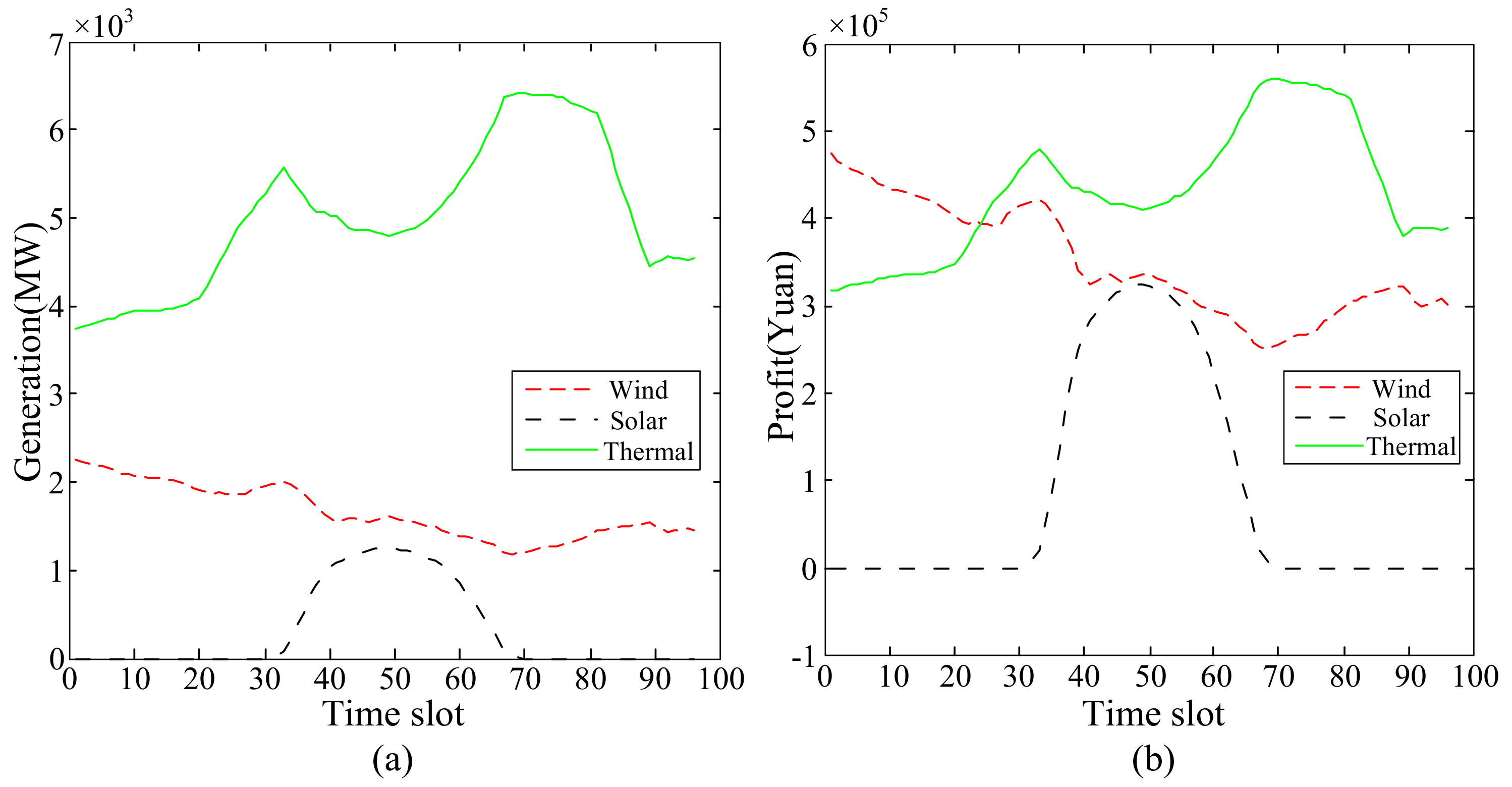
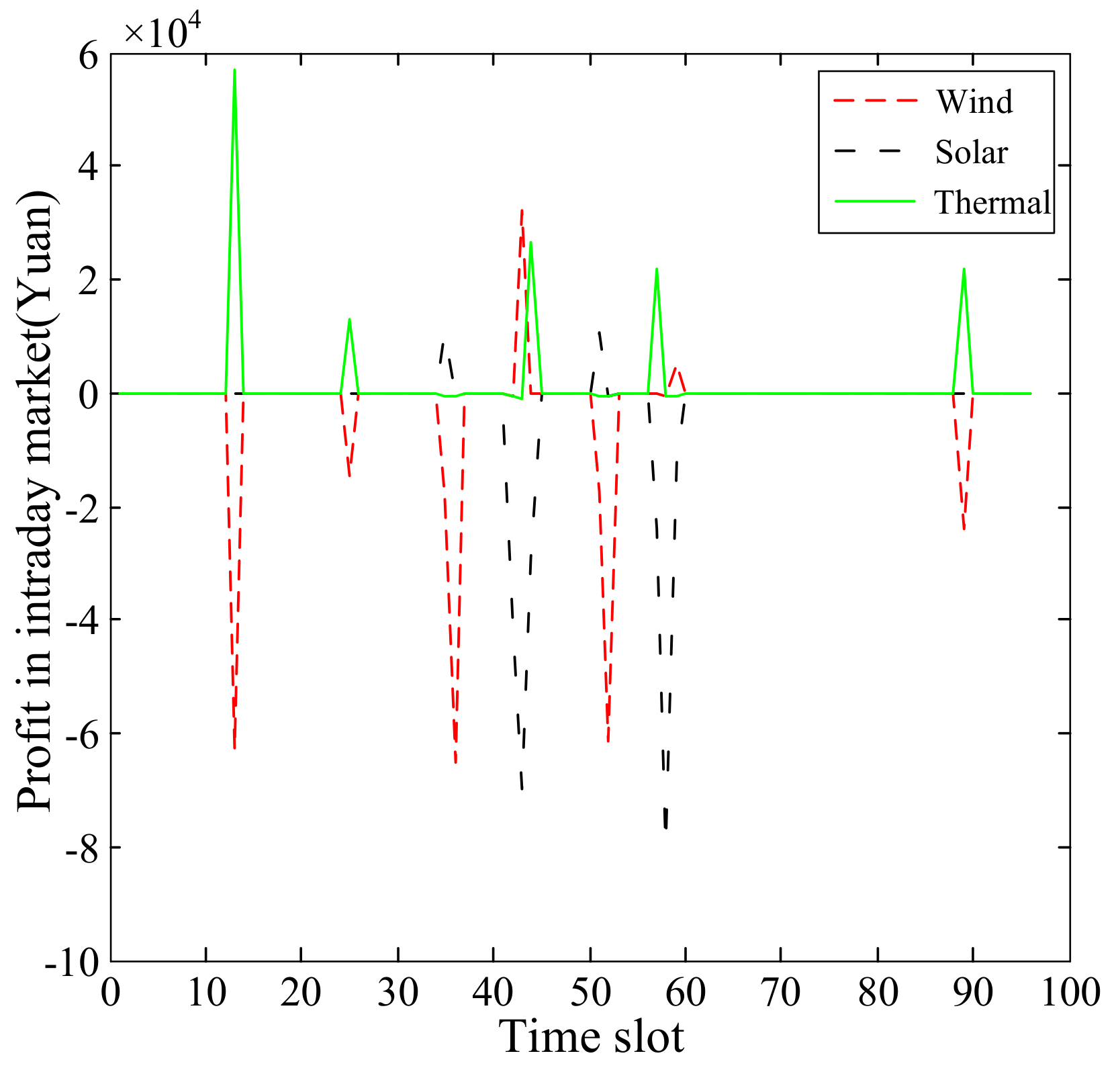
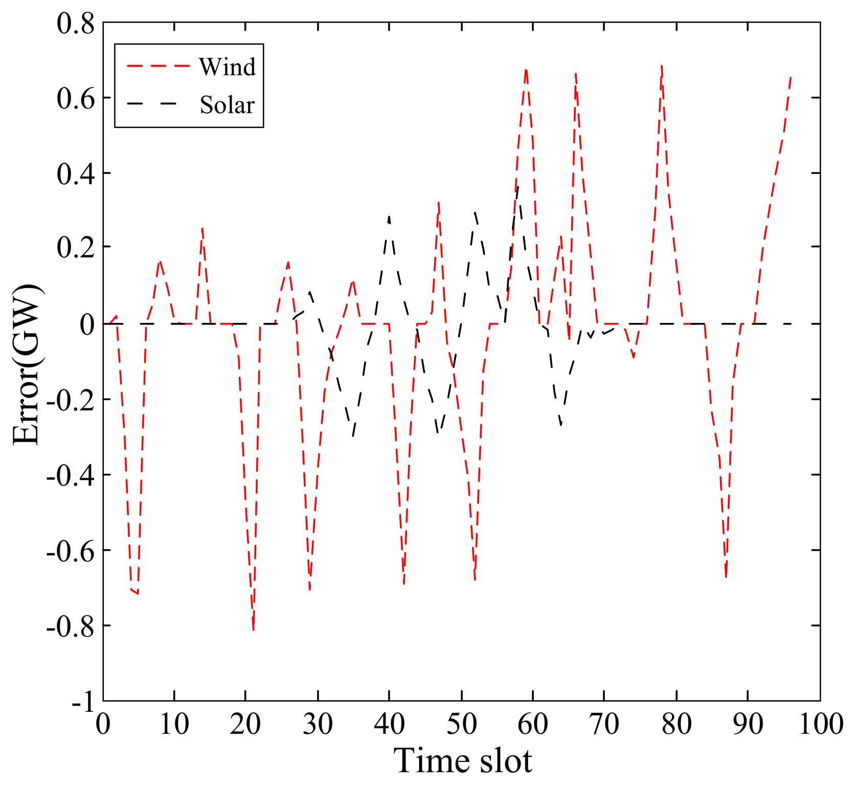
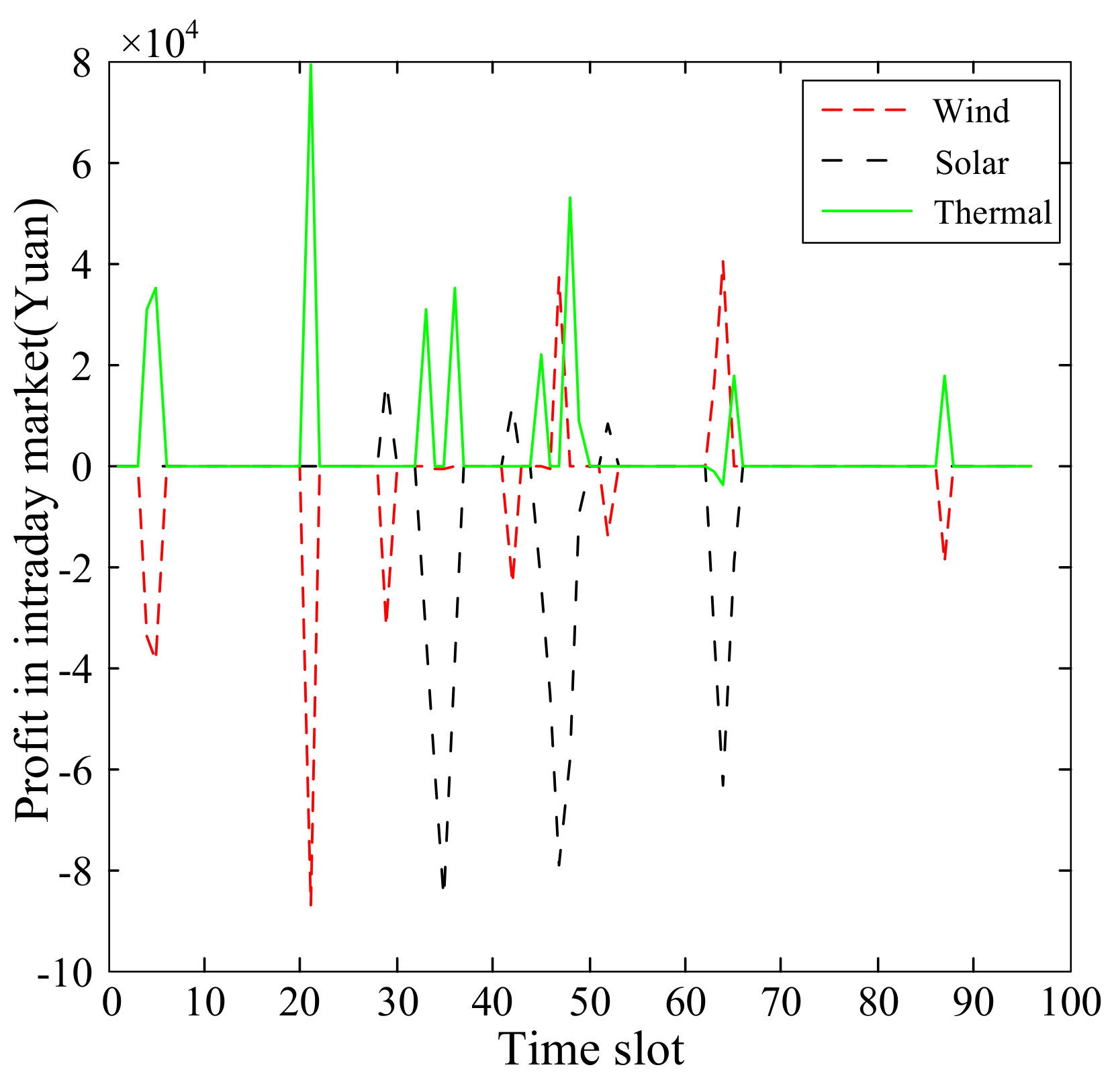
5.1. Simulation in Winter
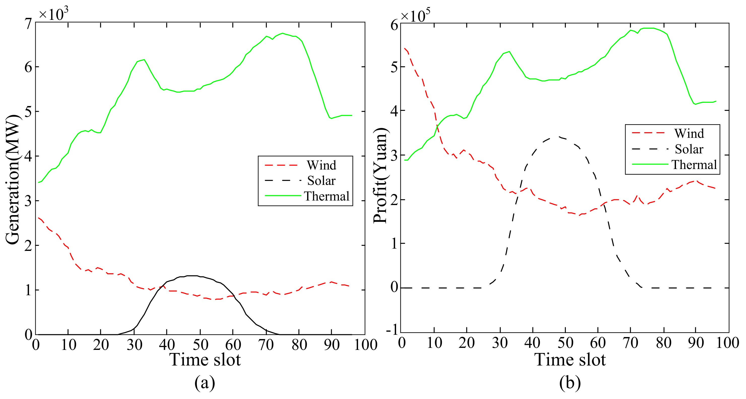
5.2. Simulation in Summer
5.3. Discussions
5.3.1. Comparison with Different Numbers of Power Plants
5.3.2. Comparison with a Different Game Approach
6. Conclusions
Acknowledgments
Author Contributions
Conflicts of Interest
References
- Liu, Z.; Zhang, Q.; Dong, C.; Zhang, L.; Wang, Z. Efficient and security transmission of wind, photovoltaic and thermal power of large-scale energy resource bases through UHVDC projects. Proc. CSEE 2014, 4, 2513–2522. (In Chinese) [Google Scholar]
- Huang, Y.; Wang, Z.; Liu, J.; Zhang, L.; Li, J. Economic analysis of wind power by UHV DC transmission. Electr. Power Constr. 2011, 32, 100–103. (In Chinese) [Google Scholar]
- Karki, R.; Hu, P.; Billiton, R. A simplified wind power generation model for reliability evaluation. IEEE Trans. Energy Convers. 2006, 21, 533–540. [Google Scholar] [CrossRef]
- Doherty, R.; O’Malley, M. A new approach to quantify reserve demand in systems with significant installed wind capacity. IEEE Trans. Power Syst. 2005, 20, 587–595. [Google Scholar] [CrossRef]
- Liu, C.; Chau, K.T.; Zhang, X. An efficient wind-photovoltaic hybrid generation system using doubly excited permanent-magnet brushless machine. IEEE Trans. Ind. Electron. 2010, 57, 831–839. [Google Scholar]
- Park, S.J.; Kang, B.B.; Yoon, J.P.; Cha, I.S.; Lim, J.Y. A Study on the stand-alone operating or photovoltaic/wind power hybrid generation system. In Proceedings of the 35th Annual Power Electronics Specialists Conference, Nanjing, China, 20–25 June 2004; pp. 1631–1634. [Google Scholar]
- Azizipanah-Abarghooee, R.; Niknam, T.; Bina, M.A.; Zare, M. Coordination of combined heat and power-thermal-wind-photovoltaic units in economic load dispatch using chance-constrained and jointly distributed random variables methods. Energy 2015, 79, 50–67. [Google Scholar] [CrossRef]
- National Energy Administration. Implementation Opinions on Expanding Renewable Energy Consumption and Promoting Sustained and Healthy Development of Renewable Energy Generation. Available online: http://www.nea.gov.cn/2016-07/20/c_135527502.htm (accessed on 23 July 2017).
- Ummels, B.C.; Gibescu, M.; Pelgrum, E.; Kling, W.L.; Brand, A.J. Impacts of wind power on thermal generation unit commitment and dispatch. IEEE Trans. Energy Convers. 2007, 22, 44–51. [Google Scholar] [CrossRef]
- Wei, Q.; Guo, W.; Tang, Y. A new approach to decrease reserve demand when bulky wind power or UHV is connected. In Proceedings of the 2012 IEEE International Conference on Power System Technology, Auckland, New Zealand, 30 October–2 November 2012; pp. 1–5. [Google Scholar]
- Shukla, A.; Singh, S.N. Cluster based wind-hydro-thermal unit commitment using GSA algorithm. In Proceedings of the 2014 IEEE PES General Meeting| Conference & Exposition, National Harbor, MD, USA, 27–31 July 2014; pp. 1–5. [Google Scholar]
- Khodayar, M.E.; Shahidehpour, M.; Wu, L. Enhancing the dispatchability of variable wind generation by coordination with pumped-storage hydro units in stochastic power systems. IEEE Trans. Power Syst. 2013, 28, 2808–2818. [Google Scholar] [CrossRef]
- Wang, Z.; Liu, L.; Liu, Z.; Wang, S.; You, Z. Optimal configuration of wind-coal power capacity and DC placement based on quantum PSO algorithm. Proc. CSEE 2014, 34, 2055–2062. (In Chinese) [Google Scholar]
- Liu, W.; Ling, Y.; Zhao, T. Cooperative game based capacity planning model for wind power in low-carbon economy. Autom. Electr. Power Syst. 2015, 39, 8–74. (In Chinese) [Google Scholar]
- Xu, D.; Wang, B.; Zhang, J.; Li, W. Integrated transmission scheduling model for wind-photocoltaic-thermal power by ultra-high voltage direct current system. Autom. Electr. Power Syst. 2016, 40, 25–29. (In Chinese) [Google Scholar]
- Zhou, W.; Peng, Y.; Sun, H. Optimal wind-thermal coordination dispatch based on risk reserve constraints. Eur. Trans. Electr. Power 2011, 21, 740–756. [Google Scholar] [CrossRef]
- Chen, C.L. Simulated annealing-based optimal wind-thermal coordination scheduling. IET Gener. Transm. Distrib. 2007, 1, 447–455. [Google Scholar] [CrossRef]
- Xia, Y.; Kang, C.; Chen, T.; Li, Y. Day-ahead market mode with power consumers participation in wind power accommodation. Autom. Electr. Power Syst. 2015, 39, 120–126. [Google Scholar]
- Sun, H.; Zhang, L.; Xu, H.; Wang, L. Mixed integer programming model for microgrid intra-day scheduling. Autom. Electr. Power Syst. 2015, 39, 21–27. [Google Scholar]
- Matevosyan, J.; Soder, L. Minimization of imbalance cost trading wind power on the short-term power market. IEEE Trans. Power Syst. 2006, 21, 1396–1404. [Google Scholar] [CrossRef]
- Skajaa, A.; Edlund, K.; Morales, J.M. Intraday trading of wind energy. IEEE Trans. Power Syst. 2015, 30, 3181–3189. [Google Scholar] [CrossRef]
- Zhang, G.; Zhang, G.; Gao, Y.; Lu, J. Competitive strategic bidding optimization in electricity markets using bilevel programming and swarm technique. IEEE Trans. Ind. Electron. 2011, 58, 2138–2146. [Google Scholar] [CrossRef]
- Fang, X.; Li, F.; Wei, Y.; Azim, R.; Xu, Y. Reactive power planning under high penetration of wind energy using Benders decomposition. IET Gener. Transm. Distrib. 2015, 9, 1835–1844. [Google Scholar] [CrossRef]
- Li, T.; Shahidehpour, M. Strategic bidding of transmission-constrained GENCOs with incomplete information. IEEE Trans. Power Syst. 2005, 20, 437–447. [Google Scholar] [CrossRef]
- Sharma, K.C.; Bhakar, R.; Padhy, N.P. Stochastic cournot model for wind power trading in electricity markets. In Proceedings of the Power and Energy Society General Meeting, National Harbor, MD, USA, 27–31 July 2014; pp. 1–5. [Google Scholar]
- Zhang, H.; Gao, F.; Wu, J.; Liu, K.; Zhai, Q. A stochastic cournot bidding model for wind power producers. In Proceedings of the IEEE International Conference on Automation and Logistics, Chongqing, China, 15–16 August 2011; pp. 319–324. [Google Scholar]
- Zhao, Z.; Li, Z.; Yao, X. Study on cost price of wind power electricity based on the certified emission reduction income. Renew. Energy Resour. 2014, 32, 662–667. (In Chinese) [Google Scholar]
- Kang, C.; Du, E.; Zhang, N. Renewable energy trading in electricity market: Review and prospect. IEEE Trans. Power Syst. 2009, 24, 1457–1468. (In Chinese) [Google Scholar]
- Sorknaes, P.; Andersen, A.N.; Tang, J.; Strom, S. Market integration of wind power in electricity system balancing. Energy Strategy Rev. 2013, 1, 174–180. [Google Scholar] [CrossRef]
- Mohsenian-Rad, A.H.; Wong, V.W.S.; Jatskevich, J.; Schober, R.; Leon-Garcia, A. Autonomous demand-side management based on game-theoretic energy consumption scheduling for the future smart grid. IEEE Trans. Smart Grid 2010, 1, 320–331. [Google Scholar] [CrossRef]
- Wang, J.; Shahidehpour, M.; Li, Z. Contingency-constrained reserve requirements in joint energy and ancillary services auction. IEEE Trans. Power Syst. 2009, 24, 1457–1468. [Google Scholar] [CrossRef]


| Parameters | Values | Parameters | Values | Parameters | Values |
|---|---|---|---|---|---|
| H | 96 | 1.1 | (Yuan/MWh) | 0.0035 | |
| (%) | 8.4 | (t/MWh) | 1.3 | (Yuan/MWh) | 116.99 |
| (Yuan/t) | 200 | (Yuan/t) | 100 | (Yuan) | 1533.06 |
| (%/min) | 2 | (%/min) | 2 | (Yuan/MWh) | 0.018 |
| (Yuan/MWh) | 215 | (Yuan/MWh) | 420 | (Yuan) | 2490 |
| (Yuan/MWh) | 104 | (Yuan/MWh) | 0.007 | (Yuan/MWh) | 0.023 |
| (Yuan/MWh) | −0.2427 | (Yuan/MWh) | −0.328 | (Yuan) | 2187 |
| Power Plant | Wind | Solar | Thermal |
|---|---|---|---|
| Maximum generating volume (MWh) | |||
| Optimal trading volume (MWh) | |||
| Optimal profit (Yuan) | |||
| Initial profit (Yuan) |
| Power Plant | Profit in Intraday Market (Yuan) | Total Profit (Yuan) | Total Generating Volume (MWh) |
|---|---|---|---|
| Wind | |||
| Solar | |||
| Thermal |
| Power Plant | Wind | Solar | Thermal |
|---|---|---|---|
| Maximum generating volume (MWh) | |||
| Optimal trading volume (MWh) | |||
| Optimal profit (Yuan) | |||
| Initial profit (Yuan) |
| Power Plant | Profit in the Intraday Market (Yuan) | Total Profit in Summer (Yuan) | Total Profit in Winter (Yuan) |
|---|---|---|---|
| Wind | |||
| Solar | |||
| Thermal |
| Number of Power Plants | Running Time of Proposed Algorithm (s) |
|---|---|
| 3 | 4.3 |
| 4 | 61.7 |
| 5 | 256.1 |
| Power Plant | Cooperative Game in Winter | Non-Cooperative Game in Winter | Cooperative Game in Summer | Non-Cooperative Game in Summer |
|---|---|---|---|---|
| Wind | ||||
| Solar | ||||
| Thermal | ||||
| Total profit |
© 2017 by the authors. Licensee MDPI, Basel, Switzerland. This article is an open access article distributed under the terms and conditions of the Creative Commons Attribution (CC BY) license (http://creativecommons.org/licenses/by/4.0/).
Share and Cite
Yuan, T.; Ma, T.; Sun, Y.; Chen, N.; Gao, B. Game-Based Generation Scheduling Optimization for Power Plants Considering Long-Distance Consumption of Wind-Solar-Thermal Hybrid Systems. Energies 2017, 10, 1260. https://doi.org/10.3390/en10091260
Yuan T, Ma T, Sun Y, Chen N, Gao B. Game-Based Generation Scheduling Optimization for Power Plants Considering Long-Distance Consumption of Wind-Solar-Thermal Hybrid Systems. Energies. 2017; 10(9):1260. https://doi.org/10.3390/en10091260
Chicago/Turabian StyleYuan, Tiejiang, Tingting Ma, Yiqian Sun, Ning Chen, and Bingtuan Gao. 2017. "Game-Based Generation Scheduling Optimization for Power Plants Considering Long-Distance Consumption of Wind-Solar-Thermal Hybrid Systems" Energies 10, no. 9: 1260. https://doi.org/10.3390/en10091260