Layout Optimisation of Wave Energy Converter Arrays
by
 , , , and
Pau Mercadé Ruiz
1,* ,
,
Vincenzo Nava
2,3 ,
,
Mathew B. R. Topper
4,
Pablo Ruiz Minguela
2, 
Francesco Ferri
1 and
Jens Peter Kofoed
1 1
Department of Civil Engineering, Aalborg University, Thomas Manns Vej 23, 9220 Aalborg, Denmark
2
Tecnalia Research and Innovation, Energy and Environmental Division, Parque Tecnologico de Bizkaia, 48160 Derio, Spain
3
Basque Centre for Applied Mathematics BCAM, 48009 Bilbao, Spain
4
Institute for Energy Systems, The University of Edinburgh, Edinburgh EH9 3DW, Scotland, UK
*
Author to whom correspondence should be addressed.
Energies 2017, 10(9), 1262; https://doi.org/10.3390/en10091262
Submission received: 19 July 2017
/
Revised: 3 August 2017
/
Accepted: 22 August 2017
/
Published: 24 August 2017
(This article belongs to the Special Issue Marine Energy)
Abstract
:This paper proposes an optimisation strategy for the layout design of wave energy converter (WEC) arrays. Optimal layouts are sought so as to maximise the absorbed power given a minimum q-factor, the minimum distance between WECs, and an area of deployment. To guarantee an efficient optimisation, a four-parameter layout description is proposed. Three different optimisation algorithms are further compared in terms of performance and computational cost. These are the covariance matrix adaptation evolution strategy (CMA), a genetic algorithm (GA) and the glowworm swarm optimisation (GSO) algorithm. The results show slightly higher performances for the latter two algorithms; however, the first turns out to be significantly less computationally demanding.
1. Introduction
Wave energy is anticipated to contribute towards the transition to carbon-free electricity generation. The theoretical wave energy resource across the oceans is estimated to be in the order of 1–10 TW [1,2], which is in the same order as the current global electric power generation [3]. Such potential has drawn the attention of the research community, which has shown that electric power production from waves is possible [4,5,6,7]. However, wave energy is still deemed costly compared to other sources of renewable energy, such as wind or solar. This makes the technological shift from development to commercialisation progress slowly.
The integration of wave energy converters (WECs) into coastal and offshore structures is a relevant solution to reduce the cost of the electricity produced by the WECs [8,9,10,11]. Working towards the same end, arrays of WECs, also known as wave farms, are considered. Wave farms may consist of a few to tens, or even hundreds, of wave energy converters, which are placed in the same geographical location. Because the WECs are in the same location, part of the cost of installation, operation and maintenance can be shared. If each device within an array produced as much electricity as (or more than) a single device, this would result in a reduction of the cost of electricity. Conversely, if each device within an array produced less, this could result in an increase in the cost of electricity. As WEC interactions mainly depend on the orientations and distances between one another [12,13,14], the advantages of using arrays will strongly depend on the ability to design optimal arrangements.
The problem of finding optimal positions of WECs in arrays was studied in [15] and [16]. In both papers, optimal positions were chosen in order to maximise the power absorption for a given number of WECs within the context of linearised potential flow theory. In [15], arrays of heaving cylinders were optimised using a method called “parabolic intersection” and a genetic algorithm (GA), the latter producing better results, although at a higher computational cost. In [16], arrays of point absorbers were optimised using a bespoke heuristic method combined with the point-absorber approximation [17] that simplified the power calculation. The optimisation strategies developed in [15] and [16] have been proven as efficient; however, they are limited to the analysis of heaving cylinders and small WECs with respect to the wavelength, respectively.
An alternative approach was proposed in [18], in which the positioning of the WECs was based on a discretisation of the array deployment area into a number of cells, where each cell was assigned 1 or 0 depending on whether or not it contained a WEC. This array representation was then used to develop a binary GA. Unlike in [15,16], optimal positions were chosen to minimise the ratio of cost to power. The method developed in [19] was used to simplify the power calculation, without further assumptions than those associated with linearised potential flow theory. The cost was modelled as proportional to the square root of the number of WECs on the basis of preliminary array cost results from Sandia National Laboratories’s Reference Model Project (RMP) [20]. Because the developed GA could only handle a fixed number of WECs, minimising the ratio of cost to power was therefore the same as maximising the power, as was employed in [15,16].
The present work has been carried out in cooperation with the research project DTOcean (Optimal Design Tools for Ocean Energy Arrays) [21], which has developed a set of tools [22] that provide optimal design solutions for arrays of wave and tidal devices. Several design aspects, such as the array layout, the electrical network, moorings/foundations, the lifecycle logistics and installation and maintenance, are considered simultaneously within DTOcean’s software to minimise the cost of electricity.
This paper focuses only on the layout optimisation of WEC arrays and demonstrates the effectiveness of the optimisation strategy adopted by DTOcean’s software. As in [15,16], optimal positions are chosen to maximise the power absorption; however, here, the number of WECs is not predefined. Instead, q-factors, the distances between the WECs, and the deployment area are constrained, which is a more realistic approach for the design of WEC arrays than using a predefined number of WECs. The first two are constrained by a minimum threshold, and the last, by a set of limiting areas. Similarly to [18], the method developed in [19] is used for an efficient power calculation. Moreover, the WECs’ positioning is based on a four-parameter array layout description that simplifies the optimisation problem. Three different optimisation algorithms are presented and further compared, namely, the covariance matrix adaptation evolution strategy (CMA) [23], a GA, and the glowworm swarm optimisation (GSO) [24]. The first is the optimisation algorithm implemented into DTOcean’s software, the second is the current standard for array layout optimisation because of its robustness [15,18], and the last has been shown to be particularly suited for optimisation problems with multiple local optima, such as in the present case.
Because the array layout optimisation strategy presented here is part of a bigger optimisation scheme that also takes into account other array design aspects, the decisions taken on the considered methods have been driven by easy integration and computational efficiency. The power calculation benefits from the fastest approach developed so far [19] within the range of validity defined by linearised potential flow theory [25]. The constraints on the q-factor, the distances between WECs, and the deployment area make up the means by which DTOcean’s software takes into account other design aspects’ effects on the array layout. The four-parameter array layout description significantly reduces the problem’s dimensionality, while it is in line with the regularity displayed by optimal solutions in previous studies [15,16,18]. The optimisation methods tested herein have been chosen as they need neither derivatives nor prior knowledge about the objective function’s behaviour. Derivatives would have to be approximated by finite differences, which would be computationally costly and would lead to approximation errors. Prior knowledge about the objective function’s behaviour could be accounted for if the optimiser was meant for a specific WEC, as in [15,16], however, the present optimiser is intended to deal with any type of WEC.
The work presented in this paper is structured into seven sections. Section 2 provides a brief description of the wave–WEC array interaction model and the equations used to calculate the absorbed power. Section 3 formulates the array layout optimisation problem and presents the strategy to solve it. Section 4 provides the details for modelling surging barges and the wave climate for the island of Île d’Yeu in France. Section 5 discusses the array layout optimisation results in terms of performance, computational effort and optimal array layout solutions. Finally, Section 6 summarises the main finding of the paper.
2. Array Power Absorption
In this section, the main equations for the prediction of the average power absorbed by an array of floating WECs over a year are presented. This will be referred to as “yearly power production” and it will be used further to select optimal array layouts (Section 3).
The equations are developed under the following considerations:
- The main forces are due to the action of gravity, the power take-off (PTO) system, and the interaction between the waves and the WECs.
- The forces are computed within the context of linearised potential flow theory, a constant water depth, and small amplitude motions compared to the wavelength and the water depth.
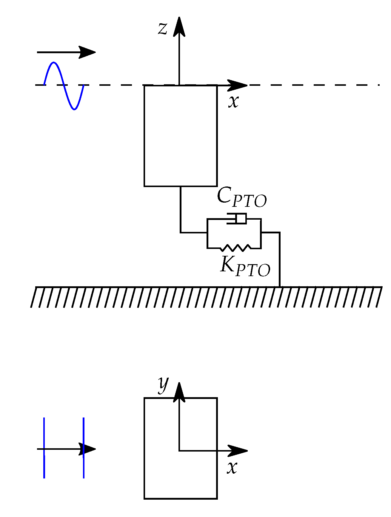
- The PTO is represented separately for each mode of motion in the array as a linear damper and a spring in parallel.
Here, the PTO system refers to the set of mechanisms whereby the motion of the WEC is transformed into electrical energy.
The equations of motion associated with the array of floating WECs when excited by a unit-amplitude plane wave with frequency follow from Newton’s second law:
where the vector contains the complex amplitude for every mode of motion in the array (), M is the mass matrix, is the added mass matrix, is the radiation damping matrix, is the PTO damping matrix, is the hydrostatic stiffness matrix, is the PTO stiffness matrix, is the diffraction force vector (), is the imaginary unit, and t is time. Both and are diagonal matrices according to the separate PTO models for each mode of motion in the array; is the force due to the action of gravity, is the force due to the action of the PTO system, is the force due to the interaction between the plane wave and the WECs at rest, and is the force due to the motion of the WECs in still water.
The power absorbed by the array of WECs from that unit-amplitude plane wave is calculated as the power dissipated through the PTO dampers. The mean absorbed power over the period can then be expressed as
where indicates the conjugate transpose of .
Given a sea state discretised by a finite number of equally spaced wave frequencies , where is the constant increment of the discretisation and ; and being characterised by its variance spectrum , where A denotes the amplitude of the wave, denotes the peak period and denotes the significant wave height; the mean absorbed power over the period can be calculated through
Given the probability of occurrence over a year for each sea state at the site at which the WECs are to be deployed, the yearly power production results from
If wave directionality is considered for sea-state characterisation, Equations (3) and (4) must also sum over the considered range of wave directions using a directional spreading function and associated probabilities, respectively.
In addition to the yearly power production, another important measure when optimising the array layout is the q-factor. Given an array of N WECs, this is defined as the ratio of the wave power absorbed by the array to N times that produced by a single-WEC array :
The denominator in the q-factor provides the total power that would be produced if the WECs were not interacting. Therefore, a q-factor smaller than 1 indicates that the hydrodynamic interactions between the WECs have an overall negative effect on the power absorption of the array, whilst a q-factor greater than 1 shows otherwise.
The added mass matrix , the radiation damping matrix , and the diffraction force vector are computed using the exact algebraic method developed in [26], known as the direct matrix method, and the numerical strategy described in [19], combined with the open-source boundary element method software NEMOH [27]. The first is used to solve the hydrodynamic interactions between the WECs, while the second is used to provide the first with the hydrodynamic response of one WEC in isolation.
Given a local analytical representation of the outgoing wave-field outside the WECs as an infinite sum of cylindrical partial waves, an interaction theory is formulated in [26] that enables the solving of the amplitudes of every cylindrical partial wave at every WEC simultaneously (direct matrix method). On the basis of the assumption of linear waves, the interaction theory constructs the local incoming wave-field outside the WECs as a superposition of outgoing waves generated by the other WECs. Finally, a linear transformation between incoming and outgoing wave amplitudes of one WEC in isolation, therein called the “diffraction transfer matrix”, is suggested in [26] to fully determine the solution of the interaction problem. The derivation of the WEC’s diffraction transfer matrix from standard boundary element method codes, such as NEMOH [27], and the derivation of wave forces, and , from the wave amplitudes are further facilitated by the strategy proposed in [19].
The use of the direct matrix method [26] and the strategy described in [19] turns out to be less computationally demanding than using NEMOH to solve the entire array. As most of the computational effort when evaluating P is put into the calculation of , and , the use of the direct matrix method [26] and the strategy described in [19] significantly reduces the overall computational cost of the optimisation process.
3. Optimisation Problem
The optimisation problem is stated as “finding the number N and position of WECs over the area of interest , maximising the yearly power production P subject to a minimum q-factor and a minimum WECs’ inter-distance ”:
where are Cartesian coordinates of the position of WEC i, and is the distance between WECs i and j.
Alternatively, if the number of WECs is held fixed to , substituting Equation (5) in the optimisation problem of Equation (6) yields
which is the way the problem has commonly been posed in the layout optimisation of WEC arrays [15,16].
The number of WECs can have a strong impact on the overall cost of the project, and thus it seems reasonable to consider this for optimisation. Nonetheless, in order to prevent the array layout solution from growing infinitely large, the area of allowed deployment is limited by . This in turn has the advantage of facilitating the implementation of the lease area associated with the wave energy project. In addition, limits are also set on the minimum separation between the WECs and the q-factor to prevent the array layout solution from overfilling.
3.1. Array Layout Description
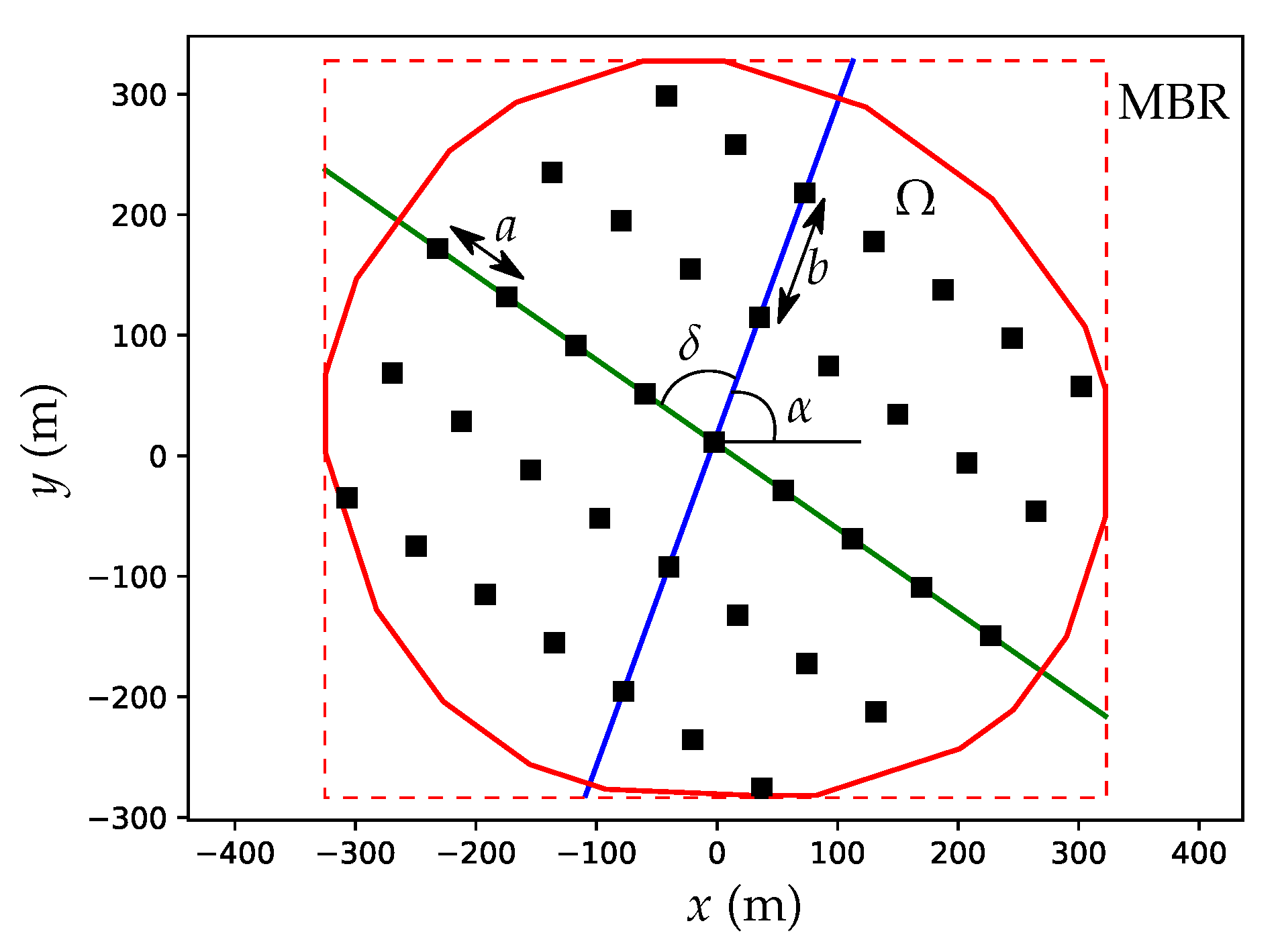
We consider a structured array arranged using rows and columns, where the WECs are placed on the intersections (Figure 1). Such array layouts can be parametrised according to the following four parameters:
- a: distance between rows.
- b: distance between columns.
- : row’s angle with respect to the x-axis.
- : angle between rows and columns.
The x-axis is assumed to be aligned with the main direction of propagation of the ambient waves, and the y-axis is the perpendicular direction to it. If wave directionality is considered for sea-state characterisation, the main direction of propagation associated with the highest probability of occurrence is chosen.
Given the minimum bounding rectangle (MBR) containing the area of deployment , the WEC array is generated by placing a WEC at the southwestern corner of that rectangle and drawing rows and columns until the number of WECs in remains unchanged; that is, until is fully filled by WECs. The total number of WECs, N, is thereby determined by , a, b, and .
The optimisation problem of Equation (6) can then be rewritten as
where D is the largest side of the MBR and f is a penalty function such that
The parameter can be adjusted to improve the performance of the optimiser. By reducing , the optimiser is less reluctant to explore the region , whereas by increasing , the more reluctant it becomes. As shown in Section 5, optimal solutions are found close to the region . Hence, should be chosen so as to allow the optimiser to search nearby that region while still producing optimal layouts satisfying the condition . It was found that normally led to a good compromise, and so this has been set as the default value.
The upper and lower bounds in the search space (Equation (8)) define a four-dimensional bounding box. These are chosen to prevent array layout repetition and to assure the minimum allowed distance between WECs. To prevent rounding errors and to generalise the optimisation problem, the following normalisation is advised:
When applying the penalty function, , normalisation by , that is, , is also advised to prevent rounding errors and to generalise the optimisation problem; may be interpreted as the array’s “effective” number of WECs—that is, the array’s number of WECs producing .
Overall, the optimisation problem reduces to maximising inside the box :
3.2. Covariance Matrix Adaptation Evolution Strategy
The CMA [23] acts on populations of individuals:
such that each individual is assigned a point in the search space and a fitness value, i.e., the objective function evaluated at that point. The population then evolves in an attempt to produce better individuals at each generation g (iteration), that is to produce individuals with larger fitness values.
The CMA generates the individuals of the population by sampling the search space assuming the population is normally distributed:
with mean and covariance matrix . Adaptation of the population implies updating the mean and the covariance matrix at each generation so that better individuals are more likely to be generated at later generations. Successful adaptations of the mean and the covariance matrix are achieved by maximising the likelihood of the best individuals and the directions of greatest improvement found at each generation, respectively. For a detailed description of the equations involving the updating of the mean and the covariance matrix, the reader is referred to [23].
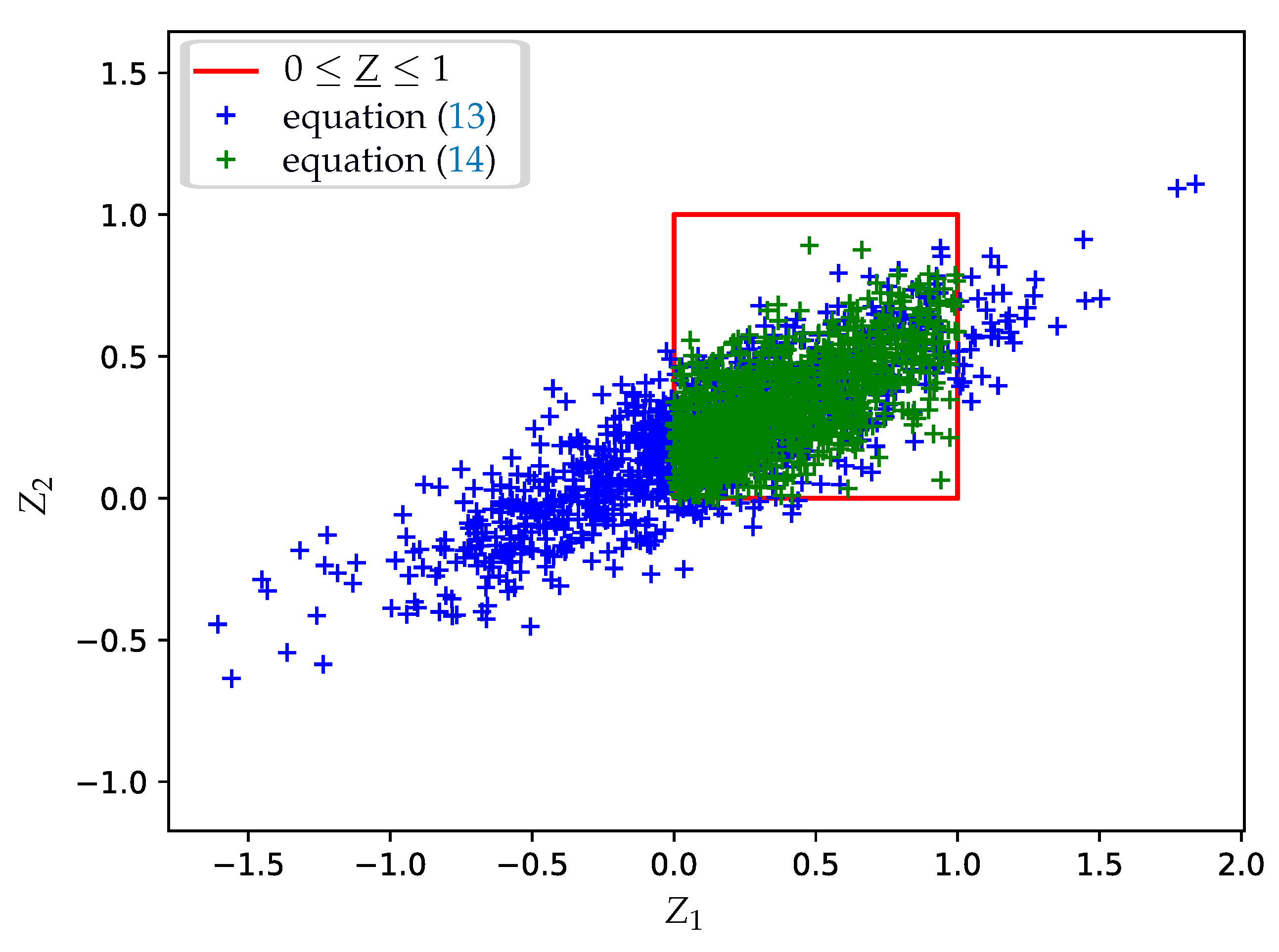
The adaptation strategy is therefore underpinned by a maximum-likelihood principle assuming a normally distributed population. In order to guarantee normality as well as to ensure individuals are generated inside the box , a truncated multivariate normal distribution [28] (Figure 2) is used instead:
The CMA algorithm [23] can be summarised into six steps:
- Initialise , and .
- Generate a population of individuals using Equation (14).
- Evaluate the objective function and set fitness value to all individuals.
- Update , and from the generated population [23].
- If any termination condition is met, go to the next step; otherwise repeat steps 2–5.
- Retrieve the best encountered individual (optimal solution) and finish.
The following termination conditions have been used:
- The objective function has been evaluated more than times.
- The standard deviation of a, b, and are smaller than , , and , respectively.
- From generation and for every generations, the best fitness value has not been improved in the last generations (stagnation), where is the closest integer to .
3.3. Genetic Algorithm
Similarly to the CMA, the GA acts on populations of individuals, as described by Equation (12). Each individual is associated with a point in the search space and with a fitness value. The main goal of the GA is then to produce better individuals at each generation.
In the GA, the () best individuals of the population are selected to breed the next generation of individuals:
where stands for the th best individual in the population and is the reproduction operator, which performs the following operations:
- Select two individuals (parents) from with associated probabilities .
- Create a new individual as a copy of the parent with the largest fitness value.
- Change parameters of the new individual by those of the parent with the smallest fitness value (crossover); is a random choice between 1 and 2. Which parameter is swapped is a random choice among a, b, and . The random choice is performed assuming a uniform distribution over all possible options without replacement.
- Change a parameter of the new individual by a random value uniformly distributed within the box (mutation), or change nothing. Whether or not mutation occurs is a random choice with associated probabilities of 0.7 or 0.3, respectively. Which parameter mutates is a random choice among a, b, and .
The GA algorithm is summarised into the following steps:
- Initialise population of individuals.
- Evaluate objective function and set fitness value to all individuals.
- Select the best individuals.
- Generate population of individuals from the best individuals using Equation (15).
- If any termination condition is met, go to the next step; otherwise repeat steps 2–5.
- Retrieve the best encountered individual (optimal solution) and finish.
The following termination conditions have been used:
- The objective function has been evaluated more than times.
- From generation and for every generations, the best fitness value has not been improved in the last generations (stagnation), where is the closest integer to .
The population size used in this paper was 10 times the number of dimensions of , and
This choice of parameters was inspired by that proposed in [23] and was tested in a number of different benchmark optimisation problems to improve the performance of the optimiser.
3.4. Glowworm Swarm Optimisation
The GSO [24] acts on populations of glowworms, described by Equation (12). Each glowworm is associated with a position in the search space and a “luciferin level” L, that is, a luminescence quantity proportional to the value of the objective function at that position:
The main goal of the GSO is to allow the glowworms to move about in the search space so that at each time step t their luciferin level increases. To this end, each glowworm randomly selects a leading glowworm among its neighbours with associated probabilities
that will be followed, so that neighbours with a larger luciferin level are more likely to be followed. We let the leading glowworm for glowworm k at time t be such that at position , the next position of glowworm k then becomes
where s is a fixed step size, and is the neighbourhood range, which is updated at each time step through
The GSO algorithm [24] can be summarised into the following steps:
- Initialise population of glowworms.
- Evaluate objective function and set the luciferin level of all glowworms using Equation (17).
- Identify neighbours and calculate associated probabilities for all glowworms using Equation (18).
- Randomly select leading glowworms according to the previously calculated probabilities.
- Update glowworms’ positions using Equation (19).
- Update glowworms’ neighbourhood range using Equation (20).
- If any termination condition is met, go to the next step; otherwise repeat steps 2–7.
- Retrieve the best encountered glowworm position (optimal solution) and finish.
The following termination conditions have been used:
- The objective function has been evaluated more than times.
- From generation and for every generations, the best fitness value has not been improved in the last generations (stagnation), where is the closest integer to .
The population size used in this paper was 10 times the number of dimensions of , and the following fixed parameter values were chosen: , , , , and . For a description of the choice of parameters, the reader is referred to [24].
4. Case Study
Arrays of surging barges (Figure 3) were considered for deployment close to the island of Île d’Yeu in France, as in [12,13]. Optimal array layouts were sought assuming a square domain m, a constant water depth of 50 m, and a minimum q-factor of . As mentioned before, the x-direction is aligned with the propagation direction of the ambient waves and the y-direction is perpendicular to it.
The barges had a length of 7.85 m in the x-direction, 10 m in the y-direction and 10 m in the vertical direction (submerged length). Further, the barges required a minimum separation distance m. The motion of the array is described by N modes , where is the complex amplitude of the oscillation along the x-direction of barge i. Assuming the barges were freely floating, their mass was 785 tonnes; thus, the mass matrix tonnes, where is the N-by-N identity matrix. The hydrostatic stiffness matrix is a zero matrix. The same control strategy was assumed for all the barges; the PTO stiffness matrix was kN·m and the PTO damping matrix was kN·s·m. Both and were used in [13], the first to compensate for the null restoring hydrostatic force, and the second to maximise the yearly power production of a single isolated barge at Île d’Yeu. The added mass matrix , the radiation damping matrix , and the diffraction force vector were computed using the method described in [19].
The sea states were reproduced by utilising the JONSWAP [29] spectrum , with a peak enhancement factor of , and by a finite number of wave frequencies rad·s, where . Thus, the part of the absorbed power in Equation (3) due to and rad·s was assumed to be negligible. The probability of occurrence over a year for each sea state at Île d’Yeu is reported in Table 1.
The yearly power generated by a single barge predicted by the numerical model described in Section 2 using the specifications described in this section was 137.5 kW, and that reported in [13] was 139 kW.
The deployment area, the minimum q-factor, the minimum separation between WECs, the WEC specifications and wave conditions considered for the case study are not specific to any wave energy project; indeed, they are intended to be as generic as possible.
5. Results and Discussion
5.1. Performance of Optimisation Algorithms
The optimisation algorithms proposed in Section 3 were tested for the case study described in Section 4. In this section, the computational efficiency of each algorithm is compared, whilst in Section 5.2, the power generated by the optimal array configurations is investigated.
The CMA, the GA and the GSO were run 100 times each, thereby leading to 100 optimal layouts each. To evaluate the optimiser’s performance, the ratio of the yearly power production of each optimal layout to that of a reference layout was used. This reference (denoted by REF) was taken to be the best layout over a grid of evenly spaced points, , in the search space . Thus, the optimiser’s performance ratio is useful for indicating how rapidly each optimisation algorithm can approach a benchmark solution.
The performances of the CMA, the GA and the GSO over the 100 runs are shown in Figure 4. The best performances achieved by these were , and , respectively. Both the GA and the GSO performed similarly, showing performances of greater than for more than 50 out of the 100 optimal layouts. On the other hand, it can be seen that the CMA led to lower performances than the GA and the GSO; roughly 40 out of the 100 optimal layouts were above . With the exception of a single optimal layout, the rest of the optimal layouts produced by the GA and the GSO showed performances of greater than , while this was accomplished by about 85 out of the 100 optimal layouts produced by the CMA.
The number of evaluations of the objective function required by the optimisers prior to termination over the 100 runs are also shown in Figure 4. The better performances of the GA and the GSO can be seen to be associated with more function evaluations, when compared with the CMA. In approximately 70 out of the 100 runs, the CMA required less than 400 function evaluations before satisfying any of the termination criteria (Section 3.2), while this was the least required by the GA and the GSO before checking stagnation (Section 3.3 and Section 3.4). Both the GA and the GSO required between 400 and 800 function evaluations in approximately 85 out of the 100 runs before satisfying the stagnation condition. Thus, about 15 out of the 100 runs of the GA and the GSO were stopped because they reached the maximum allowed number of function evaluations.
The optimiser’s performance and the required number of function evaluations are known to be tightly linked with the considered population size [23]. Large populations usually lead to better performances, although they require a larger number of function evaluations before a convergence criterion is met. Here, the convergence criterion related to any of the given termination conditions that were not triggered because of a maximum allowed number of function evaluations. Thus, if a limited number of function evaluations is set, the population size can be adjusted to maximise the optimiser’s performance within that limit. This may be done by increasing the population size until the optimiser is observed not to converge within that limit.
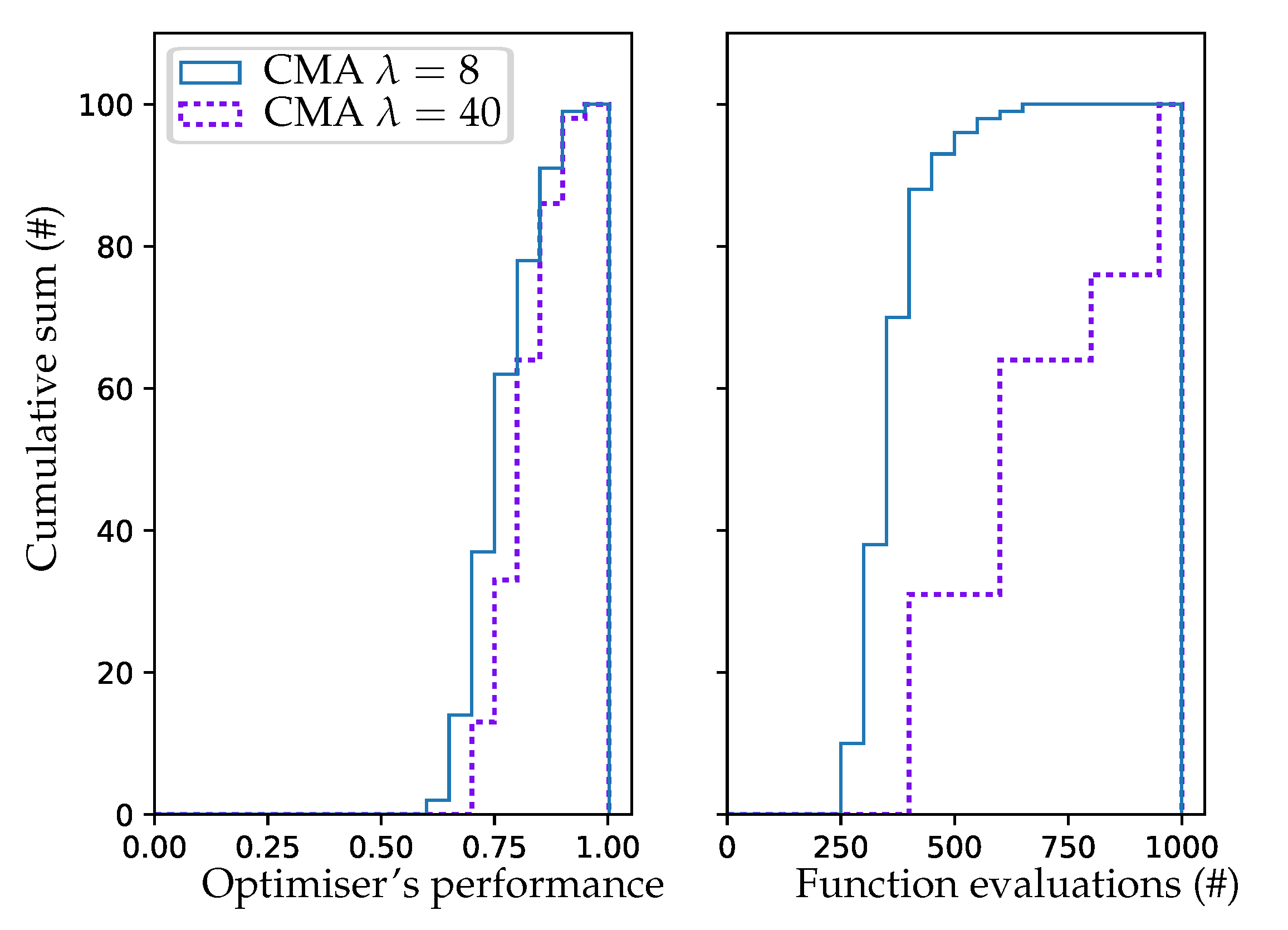
As mentioned in Section 3.2, the population sizes, as for the rest of the CMA parameters, were set according to the default values given in [23]. It seems convenient to adopt the strategy in [23] as this has been tested in a wide variety of optimisation problems. Similarly, the population size in the GA and the GSO [24] were chosen so that both optimisers performed best in a number of different benchmark optimisation problems. Given the present four-dimensional problem, the population size was set to 8 in the CMA and to 40 in the GA and the GSO. In order to evaluate the effect of a larger population size in the performance of the CMA, the simulations were repeated an additional 100 times with the same population size as for the GA and the GSO. With , the CMA exhibited performances of above for more than 65 out of the 100 optimal layouts (Figure 5). However, such improvement in performance came at the expense of computational cost. Setting a larger population size required more function evaluations in the CMA before satisfying any of the considered termination conditions. With , the CMA showed a similar trend of the distribution of the number of function evaluations in Figure 5 to those shown by the GA and the GSO in Figure 4; that is, in approximately 75 out of the 100 runs, the CMA demanded between 400 and 800 function evaluations prior to termination, while the remaining 25 runs were stopped because the maximum permitted number of function evaluations was reached. This, along with the fact that the CMA was mostly stopped as a result of stagnation, suggests that either a larger limit on the number of function evaluations or a smaller population size should be considered.
5.2. Optimal Array Layout Solutions
The best array layouts found by the CMA (with ), the GA and the GSO over the 100 runs, and the REF layout are shown in Figure 6. At first glance, all four layouts seem to have a similar configuration of parameters. Because of their apparent similarity, one may describe them as staggered arrays, where the two diagonals of the deployment area define rows and columns, that is, rad (or ) and rad.
The degree of similarity between the best layout solutions (Figure 6) can be measured by the distances between them in the parameter space, by their q-factor, and by their yearly power production (Table 2). In terms of the q-factor and yearly power production, the best layout solutions are practically the same; however, they are located several grid points away from each other with respect to the search-space discretisation used to find the REF array layout (denoted by SSD). This is illustrated in Figure 7, where the best layouts and the grid lines are projected onto the six different planes of the parameter space. The large distance between the CMA’s and the REF’s solutions is due to the fact that rows in the CMA’s layout are approximately 90 out of line compared with those in the REF’s layout. This happens to be near the limiting case in which the solution and is the same as the solution and with the role of the rows and columns swapped. With regard to the GSO’s layout, this can be seen to match the GA’s and REF’s layouts when it is mirrored with respect to the y-axis. This causes the layouts to have a similar appearance while being several grid points away from each other with respect to the SSD. Overall, it seems that the best layout solutions yield from a region in the parameter space that spans beyond grid points adjacent to the REF’s solution.
In order to study the complexity and sensitivity of the objective function, the closest grid points to the CMA’s, the GA’s and the GSO’s best layout solutions with respect to the SSD (Figure 7) were investigated. The yearly power productions generated by the arrays associated with these grid points were 2.67, 3.07 and 3.13 MW, respectively; the q-factors were 0.97, 0.89 and 0.88, respectively. The closest grid points to the GA’s and the GSO’s best layout solutions in fact violate the minimum allowed q-factor, and thus they are not feasible solutions. The closest grid point to the CMA’s best layout solution does not violate the minimum q-factor condition; however, it turns out to be associated with a significantly lower yearly power—that is, the yearly power drops from 3.22 to 2.67 MW. This is because the small variation in the array layout parameters from the CMA’s solution to its closest grid point moves the WECs that are coincident to the limits of to the exterior of the domain. These changes in the objective function value as a result of small variations along the search space provide an idea of the complexity of the present optimisation problem and its sensitivity.
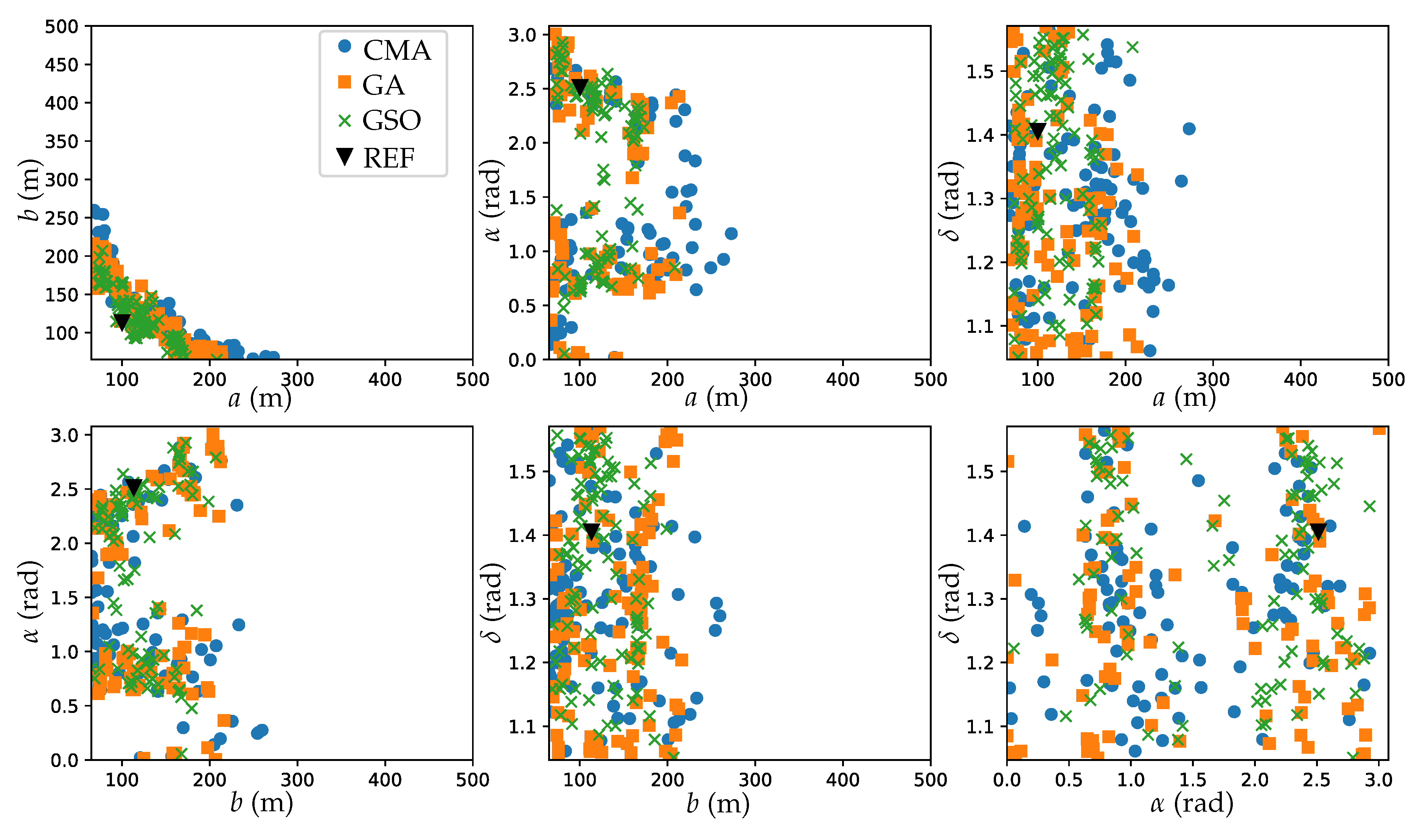
The 100 optimal array layouts found by the CMA (with ), the GA and the GSO were projected onto the six different sides of the cube defined by . The optimal distances between rows a and columns b seem to be correlated. Because the optimal solutions are constrained by a minimum q-factor, and the q-factor generally decreases with the inverse of the WECs inter-distances, if a is reduced, b is expected to increase, and vice versa; this trend can be seen in Figure 8. In addition, optimal solutions projected onto the a-b-plane concentrate close to the region m. If a smaller minimum q-factor was allowed, this region would become smaller and get closer to the origin of the a-b-plane, whereas it would become larger and approach towards the opposite corner if a larger minimum q-factor was demanded. With regard to the row’s angle , the optimal layouts appear to be characterised by either rad or , which match the angles of the two diagonals of .
The mean and the standard deviation of the q-factor for all the optimal solutions were 0.92 and 0.02, respectively. The optimal solutions were therefore found close to the region , and thus, the efficiency of the optimisers would invariably improve if they had to search solutions only within this region.
6. Conclusions
In this paper, the WEC array layout optimisation strategy implemented in DTOcean’s software has been presented. This has been described on the basis of a parametrised array layout description consisting of four parameters and an optimisation algorithm, namely the CMA [23]. In addition, two more algorithms have been introduced: a GA, which is a proven robust optimisation method [15,16], and the GSO [24], which is designed to deal especially with objective functions having multiple local maxima, as in the present case. All three optimisation algorithms were tested for the case of an array of surging barges at Île d’Yeu, that is, the same case as in [12,13].
The CMA, the GA and the GSO were compared according to their performance and computational cost. Performance was measured as the ratio of the power generated by the optimiser’s optimal solution to the power generated by the best layout encountered by direct discretisation of the search space. The computational cost was measured as the number of function evaluations required by the optimiser prior to termination. On the one hand, the performances of the GA and the GSO turned out to be very similar and slightly higher than that of the CMA, while on the other hand, the CMA led to a significantly lower computational cost than the GA and the GSO, although this equalised when using similarly sized populations. Both the performance and computational cost were seen to be sensitive to the population size considered in the optimisers. For a given maximum allowed number of function evaluations, the population size could be adjusted for a better performance of the optimiser; that is, this could be increased until the optimiser was seen to systematically stop as a result of a maximum allowed number of function evaluations.
The analyses of the best array layout solutions have revealed the degree of complexity and sensitivity of the optimisation problem. Small variations along the search space have been seen to cause significant changes in the objective function’s values. Because the area of deployment is limited, when WECs are coincident to the domain limits, a small variation in the array layout parameters may cause these to leave the domain and consequently cause the total power associated with the array to drop. Moreover, because a minimum q-factor is imposed, when array layouts are close to the constraint, forming the region in which it turns out optimal solutions tend to be, small variations in the array layout parameters may cause the array layouts to become infeasible.
Finally, observations of optimal array layout solutions have confirmed that these are likely to be found close to the limit between feasible and infeasible layouts. In this regard, significant improvements in terms of performance and computational cost could be achieved if the optimiser has only to search within that region. As this behaviour is expected regardless of the type of WEC, this could be further used to improve the implementation of the CMA algorithm or to develop a more effective optimisation algorithm.
Acknowledgments
The authors wish to thank the financial support from the European Commission (Grant No. 60859; DTOcean-Optimal Design Tools for Ocean Energy Arrays), which made this work possible. The work of Vincenzo Nava was supported by the Basque Government through the BERC 2014–2017 program and by the Spanish Ministry of Economy and Competitiveness MINECO: BCAM Severo Ochoa accreditation SEV-2013-0323.
Author Contributions
Vincenzo Nava, Mathew B.R. Topper, Pablo Ruiz Minguela and Pau Mercadé Ruiz conceived and designed the numerical tests. Pau Mercadé Ruiz performed the tests, analysed the data and wrote the paper with support, discussion and revision from Jens Peter Kofoed, Francesco Ferri, Vincenzo Nava, Mathew B.R. Topper and Pablo Ruiz Minguela.
Conflicts of Interest
The authors declare no conflict of interest.
References
- Falnes, J. A review of wave-energy extraction. Mar. Struct. 2007, 20, 185–201. [Google Scholar] [CrossRef]
- Barstow, S.; Mørk, G.; Mollison, D.; Cruz, J. The wave energy resource. In Ocean Wave Energy; Springer: Berlin, Germany, 2008; pp. 93–132. [Google Scholar]
- World energy demand and economic outlook. In International Energy Outlook 2016; U.S. Energy Information Administration: Washington, DC, USA, 2016; pp. 7–17.
- Clément, A.; McCullen, P.; Falcão, A.F.O.; Fiorentino, A.; Gardner, F.; Hammarlund, K.; Lemonis, G.; Lewis, T.; Nielsen, K.; Petroncini, S.; et al. Wave energy in Europe: Current status and perspectives. Renew. Sustain. Energy Rev. 2002, 6, 405–431. [Google Scholar] [CrossRef]
- Falcão, A.F.O. Wave energy utilization: A review of the technologies. Renew. Sustain. Energy Rev. 2010, 14, 899–918. [Google Scholar] [CrossRef]
- Magagna, D.; Uihlein, A. Wave energy. In JRC Ocean Energy Status Report; Publications Office of the European Union: Luxembourg, 2014; pp. 31–43. [Google Scholar]
- Uihlein, A.; Magagna, D. Wave and tidal current energy—A review of the current state of research beyond technology. Renew. Sustain. Energy Rev. 2016, 58, 1070–1081. [Google Scholar] [CrossRef]
- Kallesøe, B.S.; Dixen, F.H.; Hansen, H.F.; Køhler, A. Prototype test and modeling of a combined wave and wind energy conversion system. In Proceedings of the 8th European Wave and Tidal Energy Conference, Uppsala, Sweden, 7–10 September 2009; pp. 453–459. [Google Scholar]
- Iuppa, C.; Contestabile, P.; Cavallaro, L.; Foti, E.; Vicinanza, D. Hydraulic performance of an innovative breakwater for overtopping wave energy conversion. Sustainability 2016, 8, 1226. [Google Scholar] [CrossRef]
- Falcão, A.F.; Henriques, J.C. Oscillating-water-column wave energy converters and air turbines: A review. Renew. Energy 2016, 85, 1391–1424. [Google Scholar] [CrossRef]
- Contestabile, P.; Iuppa, C.; Di Lauro, E.; Cavallaro, L.; Andersen, T.L.; Vicinanza, D. Wave loadings acting on innovative rubble mound breakwater for overtopping wave energy conversion. Coast. Eng. 2017, 122, 60–74. [Google Scholar] [CrossRef]
- Babarit, A. Impact of long separating distances on the energy production of two interacting wave energy converters. Ocean Eng. 2010, 37, 718–729. [Google Scholar] [CrossRef]
- Borgarino, B.; Babarit, A.; Ferrant, P. Impact of wave interactions effects on energy absorption in large arrays of wave energy converters. Ocean Eng. 2012, 41, 79–88. [Google Scholar] [CrossRef]
- Penalba, M.; Touzón, I.; López-Mendia, J.; Nava, V. A numerical study on the hydrodynamic impact of device slenderness and array size in wave energy farms in realistic wave climates. Ocean Eng. 2017, 142, 224–232. [Google Scholar] [CrossRef]
- Child, B.F.M.; Venugopal, V. Optimal configurations of wave energy device arrays. Ocean Eng. 2010, 37, 1402–1417. [Google Scholar] [CrossRef]
- Moarefdoost, M.M.; Snyder, L.V.; Alnajjab, B. Layouts for ocean wave energy farms: Models, properties, and heuristic. Omega 2017, 66, 185–194. [Google Scholar] [CrossRef]
- Budal, K. Theory for absorption of wave power by a system of interacting bodies. J. Ship Res. 1977, 21, 4. [Google Scholar]
- Sharp, C.; DuPont, B. Wave energy converter array optimization—A review of current work and preliminary results of a genetic algorithm approach introducing cost factors. In Proceedings of the ASME 2015 International Design Engineering Technical Conference and Computers and Information in Engineering Conference, Boston, MA, USA, 2–5 August 2015. [Google Scholar]
- McNatt, J.C.; Venugopal, V.; Forehand, D. A novel method for deriving the diffraction transfer matrix and its application to multi-body interactions in water waves. Ocean Eng. 2015, 94, 173–185. [Google Scholar] [CrossRef]
- Sandia National Laboratory’s Reference Model Project (RMP). Available online: http://energy.sandia.gov/energy/renewable-energy/water-power/technology-development/reference-model-project-rmp/ (accessed on 10 June 2017).
- Nava, V.; Topper, M.B.R.; Ruiz-Minguela, P.; de Andrés, A.; Jeffrey, H. A critical discussion about optimisation approaches for ocean energy array design. In Proceedings of the 2nd International Conference on Renewable Energies Offshore (RENEW2016), Lisbon, Portugal, 24–26 October 2016; pp. 383–391. [Google Scholar]
- Optimal Design Tools for Ocean Energy Arrays (DTOcean). Available online: http://www.dtocean.eu (accessed on 10 June 2017).
- Hansen, N. The CMA Evolution Strategy: A Tutorial. arXiv 2016, 1604, 1–39. [Google Scholar]
- Krishnanand, K.N.; Ghose, D. Glowworm swarm optimization for simultaneous capture of multiple local optima of multimodal functions. Swarm Intell. 2009, 3, 87–124. [Google Scholar] [CrossRef]
- Mercadé Ruiz, P.; Ferri, F.; Kofoed, J.P. Experimental validation of a wave energy converter array hydrodynamics tool. Sustainability 2017, 9, 115–134. [Google Scholar] [CrossRef]
- Kagemoto, H.; Yue, D.K.P. Interactions among multiple three-dimensional bodies in water waves: An exact algebraic method. J. Fluid Mech. 1986, 166, 189–209. [Google Scholar] [CrossRef]
- Babarit, A.; Delhommeau, G. Theoretical and numerical aspects of the open source BEM solver NEMOH. In Proceedings of the 11th European Wave and Tidal Energy Conference, Nantes, France, 6–11 September 2015. [Google Scholar]
- Wilhelm, S.; Manjunath, B.G. Tmvtnorm: A package for the truncated multivariate normal distribution. Sigma 2010, 2, 2. [Google Scholar]
- Hasselmann, K. Measurements of wind wave growth and swell decay during the Joint North Sea Wave Project (JONSWAP). Dtsch. Hydrogr. Z. 1973, 8, 95. [Google Scholar]
Figure 1.
Array layout description. The black dots represent wave energy converter (WEC) positions. The continuous red line is the bounds of the array deployment, the blue line is a row, and the green line is a column. The x-axis is aligned with the main direction of propagation of the ambient waves.

Figure 2.
Samples generated from a truncated bivariate normal distribution.

Figure 3.
Sketch of a single barge excited by a plane wave travelling along the x-direction.

Figure 4.
Optimisers’ performance and required number of function evaluations prior to termination. The results are shown for the 100 runs performed by each optimiser.
Figure 4.
Optimisers’ performance and required number of function evaluations prior to termination. The results are shown for the 100 runs performed by each optimiser.
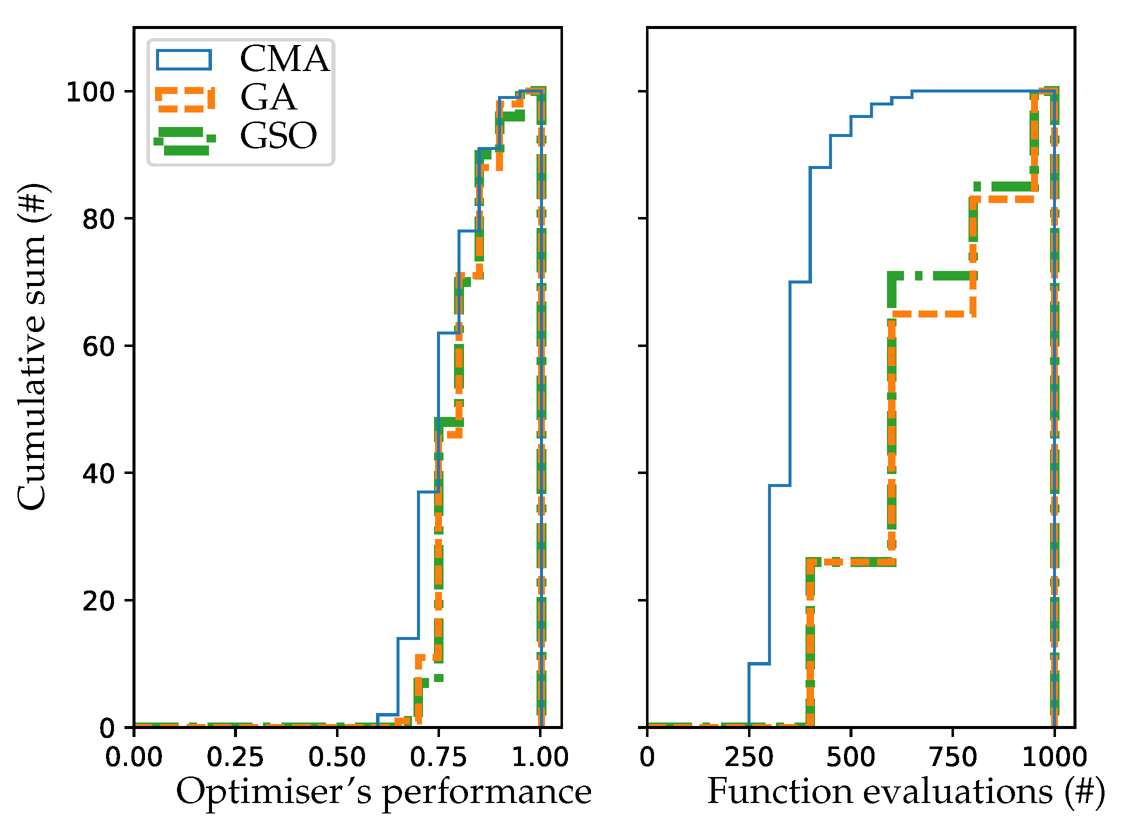
Figure 5.
Covariance matrix adaptation evolution strategy’s (CMA’s) performance and required number of function evaluations prior to termination. The results are shown for 100 runs performed using population sizes of 8 and 40.
Figure 5.
Covariance matrix adaptation evolution strategy’s (CMA’s) performance and required number of function evaluations prior to termination. The results are shown for 100 runs performed using population sizes of 8 and 40.

Figure 6.
Best array layouts found by the optimisers and the reference layout (REF).
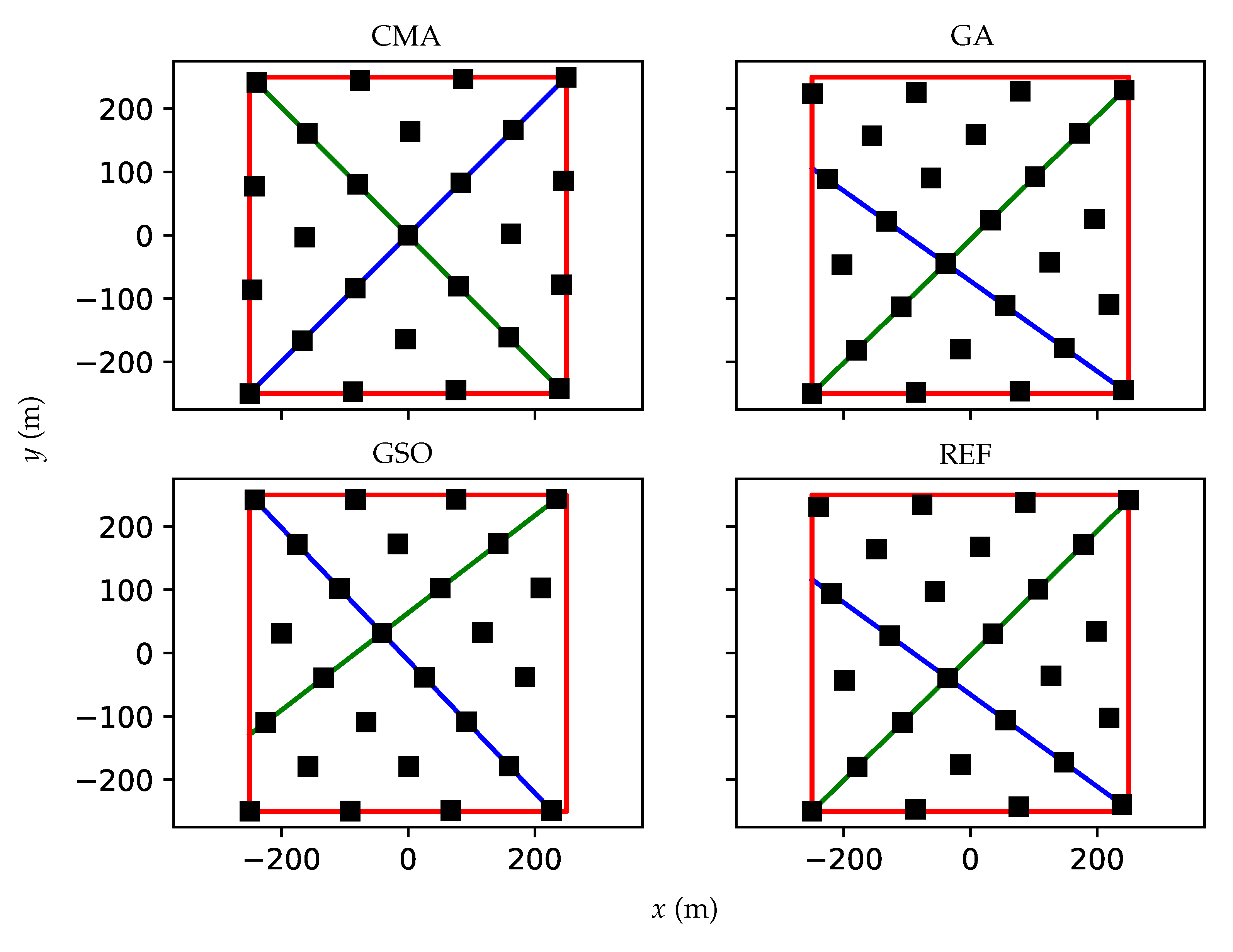
Figure 7.
Search-space discretisation (SSD), best layout parameters found by the optimisers, and the reference layout (REF) parameters. Grid points resulting from the SSD are shown as the intersections between black lines.
Figure 7.
Search-space discretisation (SSD), best layout parameters found by the optimisers, and the reference layout (REF) parameters. Grid points resulting from the SSD are shown as the intersections between black lines.
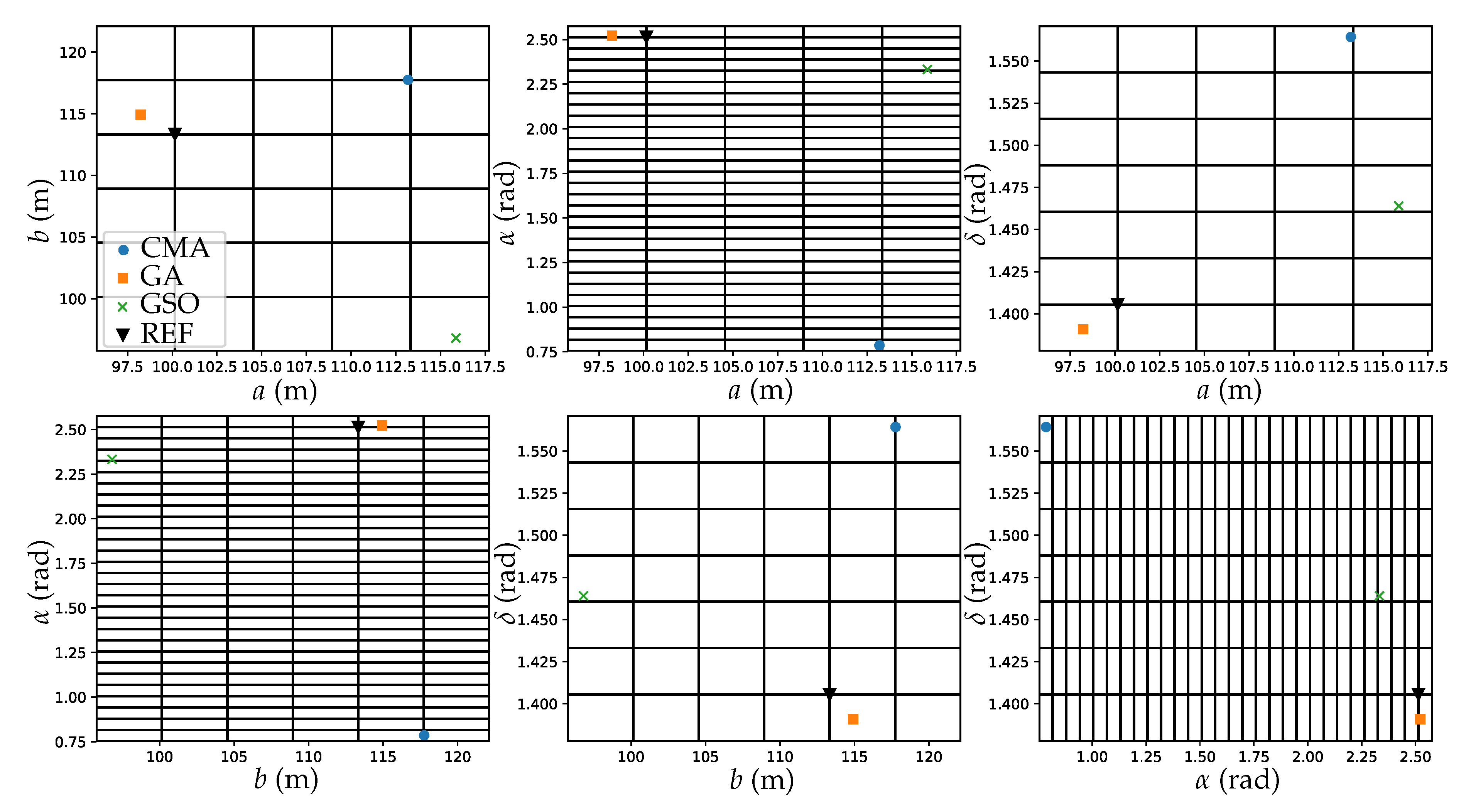
Figure 8.
Optimal layout parameters found by the optimisers over the 100 runs and the reference layout parameters (REF).
Figure 8.
Optimal layout parameters found by the optimisers over the 100 runs and the reference layout parameters (REF).


Table 2.
Distances between best layout solutions in the parameter space, their q-factor and their yearly power production.
Table 2.
Distances between best layout solutions in the parameter space, their q-factor and their yearly power production.
| Parameter | CMA | GA | GSO | REF |
|---|---|---|---|---|
| 0.63 | 0.03 | 0.14 | 0.00 | |
| q | 0.93 | 0.90 | 0.90 | 0.90 |
| P (MW) | 3.22 | 3.23 | 3.21 | 3.21 |
© 2017 by the authors. Licensee MDPI, Basel, Switzerland. This article is an open access article distributed under the terms and conditions of the Creative Commons Attribution (CC BY) license (http://creativecommons.org/licenses/by/4.0/).
Share and Cite
MDPI and ACS Style
Ruiz, P.M.; Nava, V.; Topper, M.B.R.; Minguela, P.R.; Ferri, F.; Kofoed, J.P. Layout Optimisation of Wave Energy Converter Arrays. Energies 2017, 10, 1262. https://doi.org/10.3390/en10091262
AMA Style
Ruiz PM, Nava V, Topper MBR, Minguela PR, Ferri F, Kofoed JP. Layout Optimisation of Wave Energy Converter Arrays. Energies. 2017; 10(9):1262. https://doi.org/10.3390/en10091262
Chicago/Turabian StyleRuiz, Pau Mercadé, Vincenzo Nava, Mathew B. R. Topper, Pablo Ruiz Minguela, Francesco Ferri, and Jens Peter Kofoed. 2017. "Layout Optimisation of Wave Energy Converter Arrays" Energies 10, no. 9: 1262. https://doi.org/10.3390/en10091262
Note that from the first issue of 2016, this journal uses article numbers instead of page numbers. See further details here.