
Modelling and Simulation of Electric Vehicle Fast Charging Stations Driven by High Speed Railway Systems


1
Department of Energy, Politecnico di Milano, via La Masa, 34-20156 Milano, Italy
2
CanmetENERGY Research Centre, Natural Resources Canada, 1 Haanel Drive, Ottawa, ON K1A 1M1, Canada
*
Author to whom correspondence should be addressed.
Energies 2017, 10(9), 1268; https://doi.org/10.3390/en10091268
Submission received: 26 June 2017
/
Revised: 2 August 2017
/
Accepted: 10 August 2017
/
Published: 25 August 2017
(This article belongs to the Special Issue Energy Storage Systems and Power Conversion Electronics for E-Transportation and Smart Grid)
Abstract
:The aim of this investigation is the analysis of the opportunity introduced by the use of railway infrastructures for the power supply of fast charging stations located in highways. Actually, long highways are often located far from urban areas and electrical infrastructure, therefore the installations of high power charging areas can be difficult. Specifically, the aim of this investigation is the analysis of the opportunity introduced by the use of railway infrastructures for the power supply of fast charging stations located in highways. Specifically, this work concentrates on fast-charging electric cars in motorway service areas by using high-speed lines for supplying the required power. Economic, security, safety and environmental pressures are motivating and pushing countries around the globe to electrify transportation, which currently accounts for a significant amount, above 70 percent of total oil demand. Electric cars require fast-charging station networks to allowing owners to rapidly charge their batteries when they drive relatively long routes. In other words, this means about the infrastructure towards building charging stations in motorway service areas and addressing the problem of finding solutions for suitable electric power sources. A possible and promising solution is proposed in the study that involves using the high-speed railway line, because it allows not only powering a high load but also it can be located relatively near the motorway itself. This paper presents a detailed investigation on the modelling and simulation of a 2 × 25 kV system to feed the railway. A model has been developed and implemented using the SimPower systems tool in MATLAB/Simulink to simulate the railway itself. Then, the model has been applied to simulate the battery charger and the system as a whole in two successive steps. The results showed that the concept could work in a real situation. Nonetheless if more than twenty 100 kW charging bays are required in each direction or if the line topology is changed for whatever reason, it cannot be guaranteed that the railway system will be able to deliver the additional power that is necessary.
1. Introduction
In order to meet future mobility needs, decrease greenhouse gas and toxic emissions, and eliminate dependence on fossil fuels, nowadays automotive technologies require to be substituted by further effective, efficient and clean environmentally alternative energy sources. On the evolution to a sustainable society, proficient mobility technologies are mainly desirable worldwide. Electric vehicles have been recognised as being such a technology. In parallel, some nations, like Denmark, Germany and Sweden have agreed to replace electricity production from fossil fuel to renewable energy sources, hence further advancing sustainability and viability of electric vehicles when compared with internal combustion engine vehicles.
People realised in the 1950s and 1960s that trains could compete with commercial flights if travelling time by train was shorter than by plane. Two things have to be remembered when comparing trains and planes: the location of the airports and train stations; and the boarding procedures. Most airports are on the outskirts of the city and an additional trip by public transport or taxi is required to get to the city centre, while railway stations typically are located in the city centre [1]. Boarding procedures are also very different between trains and planes. Usually the boarding procedure for trains requires getting to the station in time to catch the train and proceeding through passport control, while flying requires getting to the airport at least one hour before the flight departure for national flights (two hours when flying internationally) to dropping off luggage and passing extensive security checks in addition to passport control [2]. Flying requires time after landing as well, especially for the luggage claim, which is not needed for train travel. This means train travelling can be much faster than flying for short distance travel. An example of this is the Tokaido Shinkansen line between Tokyo and Osaka. Built in 1964, today it carries, on a daily basis, more than 400,000 passengers on average, with 330,000 available seats on limited stop trains compared to 30,000 seats of airlines capacity. This is also due to the fact trains can carry far more passengers than any airliner, making trains more energy efficient. This led other developed countries to establish their own high-speed train services and to build a high-speed network. Because of the high-power demands of high-speed trains, it became clear that traditional electrification schemes were not very good at delivering that much power, so the 2 × 25 kV autotransformer system was used for new lines and new electrifications [3,4]. This system allows for having a relatively low number of substations while delivering a lot of power to the trains, with the advantage of minimising energy losses and voltage drops [5].
The issue of climate change and greenhouse effects led governments and regulating agencies to enforce stricter emission limits on traditional internal combustion engines [6]. This led to the rediscovery of the electric car. Invented in 1830, the electric car became a research topic when it was clear that internal combustion engines were the best solution available. Recent developments in battery technology, especially the lithium ion batteries, and in electronics led to the modern electric car, which is comparable with traditional cars in terms of performance. Despite the technological developments, the long charging times mean that electric vehicles are mostly used in cities and towns [6].
The increase in popularity of electric vehicles requires the construction of a suitable fast-charging infrastructure to allow driving longer distances. Usually high-speed lines are built (or designed to be built) near existing motorways [7,8,9]. Since the best place to install fast-charging facilities are motorways service areas because the necessary services are already there, it is interesting to study the possibility of connecting these charging facilities to the neighbouring high-speed line rather than the high-voltage transmission grid [10].
Electric vehicles need to have their batteries recharged to gain extra range, just as a traditional gasoline car needs to have its tank filled up at a gasoline station. There are three ways to get the batteries charged [11,12,13]. Battery swapping consists in swapping the depleted batteries with fully charged ones. In practice, almost no current electric car (except Tesla’s) allows for it and has lost much of its appeal when a service provider went bankrupt in 2013. Wired charging brings electricity to the vehicle using cables and plugs. It is the most widely used technology. Induction charging transmits electricity through high frequency variable magnetic fields. It is still in development and it is only used in a few pilot locations [14].
The CENELEC EN 61851-1 standard on wired charging requires that the Electric Vehicle (EV) shall be connected to the EVSE (Electric Vehicle Supply Equipment) so that in normal conditions of use, the conductive energy transfer function operates safely [15,16]. In particular, the standard defines four charging modes but they are not all legal in every country. The four charging modes are: (a) Mode 1; (b) Mode 2; (c) Mode 3; and (d) Mode 4. Mode 1 charging requires connecting the EV to the Alternating Current (AC) supply network (mains) utilizing standardised socket-outlets not exceeding 16 A and not exceeding 250 V single-phase or 480 V three-phase, at the supply side, and utilizing the power and protective earth conductors [17,18,19]. Mode 2 charging requires a connection of the EV to the AC supply network (mains) not exceeding 32 A and not exceeding 250 V single-phase or 480 V three-phase utilising standardised single-phase or three-phase socket-outlets. It requires also utilising the power and protective earth conductors together with a control pilot function and system of personnel protection against electric shock (RCD) between the EV and the plug or as a part of the in-cable control box. The in-line control box needs to be located within 0:3 m of the plug or the EVSE or in the plug. Mode 3 charging requires connecting the EV to the AC supply network (mains) using dedicated EVSE where the control pilot function extends to control equipment in the EVSE, permanently connected to the AC supply network (mains). Mode 4 charging needs a connection of the EV to the AC supply network (mains) utilizing an on-board charger where the control pilot function extends to equipment permanently connected to the AC supply [20,21].
It is possible to classify the four charging modes according to the charging speed: Modes 1 and 2 are generally used for slow charging from the household plug, while Mode 4 is usually used for fast DC charging at a charging station. Mode 3, on the other hand, can be used both for slow charging and for fairly quick charging depending on the capability of the car and the infrastructure. The existence and the differences between Modes 1–3 are due to different factors: the consumer representatives want something cheap and feel that the stock household plugs are acceptable for home charging, while the industry feels that a purpose-built solution would be better thanks to higher safety and reliability.
There are three connectors standardised for AC charging: the US, Japan, and other countries that have a predominantly single-phase distribution network use the type 1 (or SAE) connector. Europe has settled on the Mennekes type 2 connector, which supports both single and three-phase power supplies up to 40 kW, and China uses its own standard. DC fast charging (Mode 4) sees a different situation, because there are four standards available on the market and the question has not been fully settled yet. The available standards are: (a) Tesla’s Supercharger [22,23]; (b) the Chinese GB/T [24,25]; (c) the Combined Charging System (CCS) [26]; and (d) the CHAdeMO [27].
The power quality analyses carried out are also useful to predict the aging of the power devices as substation transformers [28,29].
A limited number of research studies propose different concepts for EV charging stations powered by renewable energies, including architectures, control strategies and infrastructure planning [30,31,32,33,34,35,36,37]. Despite the above efforts, the authors did not find detailed information on the modelling and simulation of electric vehicle fast charging stations powered by high-speed railway lines in Italy [38,39,40]. In order to further investigate the characteristics of the concept, a model of a 2 × 25 kV system to feed the railway was proposed and simulations of the battery charger were presented in detail. It is hoped that this contribution will lead to optimisation of the system design and characterisation and to encourage its widespread improvement and applications.
Moreover, many current researchers are focused on power electronic converters and devices for automotive applications [41,42].
The aim of this work is the analysis of the opportunity introduced by the use of railway infrastructures for the power supply of fast charging stations located in highways. In fact, long highways are often located far from urban areas and electrical infrastructure; hence, the installations of high power charging areas can be problematic.
This paper is organised as follows: Section 2 presents a detailed description of the 25 kV railway electrification, dividing the section in two different parts, a focus on the configuration and design of the 2 × 25 kV systems and another focus on the mathematical model of the 2 × 25 kV system, respectively. The specifications and configuration of the charging facility used in this analysis and the simulation model of the load are given in Section 3. Section 4 provides details of the system simulation of the charging system and results. Finally, the conclusions are reported in Section 5.
2. The 25 kV Railway Electrification
2.1. Configuration and Design of the 2 × 25 kV System
The 25 kV AC single phase is the most common electrification system for new high speed lines in the variant 2 × 25 kV autotransformer feed. This electrification system is commonly used with the industrial frequency (50 or 60 Hz) but it may be used for the railway frequency as well [43].
The 25 kV electrification schemes are single-phase electrification systems that are powered from the three phase industrial grid. This poses some problems due to the unbalance that a high power single-phase load creates on the grid’s voltage. The degree of unbalance on the grid is limited to reduce the possibility of damage to generators and electric motors and it is measured though the unbalance coefficient, which is defined as follows:
where Vi is the negative sequence voltage and Vd is the positive sequence voltage. In practice, the unbalance coefficient is measured through the following Equation (2):
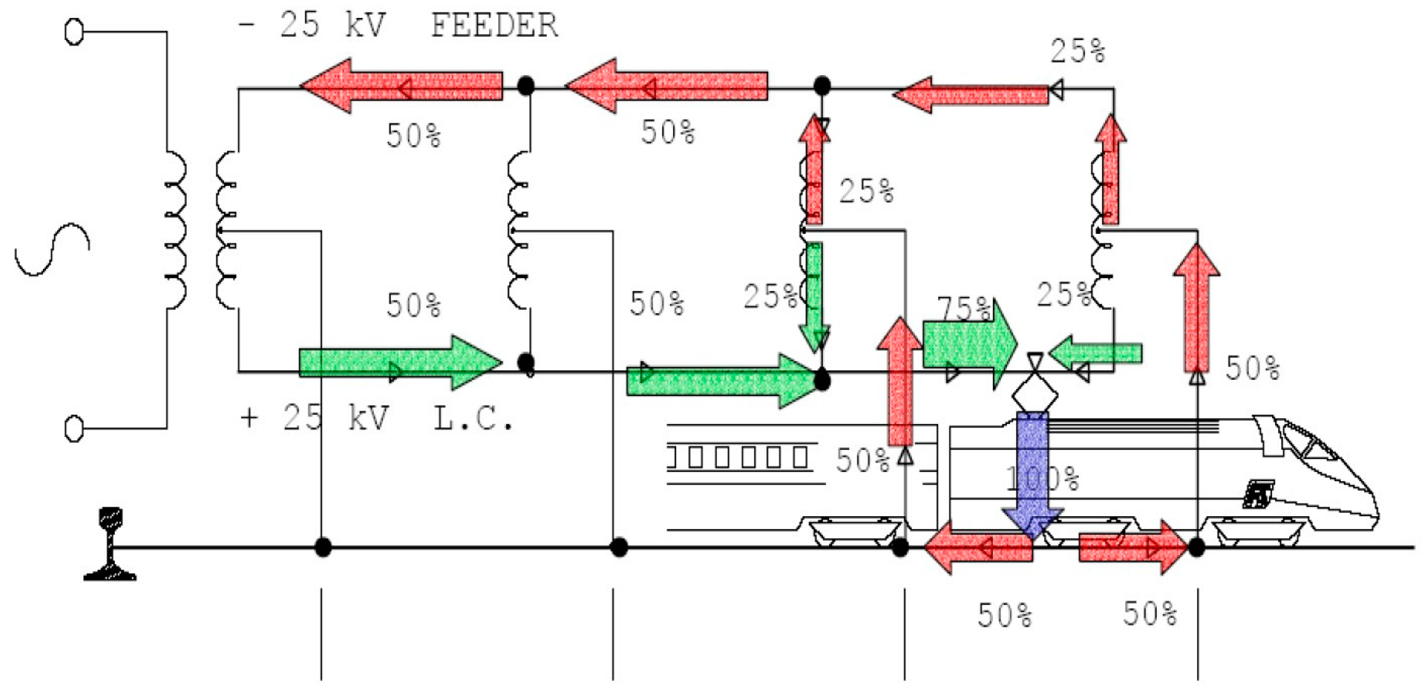
where Psp is the power of the single-phase load and Psc is the three-phase short circuit power of the connection node. International standards and transmission system operators set the maximum degree of unbalance between 1 and 2% that means that the load has to be connected to a high-voltage node with sufficiently high short-circuit-power. This later is not a problem where a high-power grid is available, but can be difficult on islands characterised by weak networks. The railway line is powered by several substations that are connected to different phase pairs in order to further reduce load unbalance on the industrial grid. Each substation is built with redundant apparatuses, such as two transformers and two connections to the industrial grid, in order to prevent the line grinding to a halt, in case of failure of any of these components. The connection between two different phase-couples of two successive ESS (energy storage system) implies that a neutral section has to be built when the power supply switches from one ESS to the next because of the voltage difference between two out-of-phase circuits. Usually, neutral sections are placed at the substations and halfway between them. Each neutral section is signalled to the engine driver to allow them to disconnect all the train loads (traction motors included) before entering the neutral section itself (Figure 1).
The neutral sections can be energised from either end when needed. International standards set the tolerance of the voltage in the system once the nominal value is chosen. The tolerances and the maximum duration allowed for a nominal voltage of 25 kV are reported in Table 1.
Low traffic lines are usually fed directly from the transformer through the over-head line and the rail as return conductor. High traffic lines and high-speed lines are usually fed with an autotransformer system because it allows building the feeding stations further apart and, consequently, to contain the costs of building high-voltage lines to connect substations to the grid. Each electrical substation has two power transformers that supply the system from the high-voltage industrial network. The distance between substations is usually between 40 and 60 km. Autotransformers are installed regularly every 10 to 15 km between two consecutive substations [45].
The railway traction supply system has to be protected against faults so circuit breakers and switches are vital to isolate the faulted section and keep the system running. The heart of the protection system is a distance protection relay whose shape varies depending on the manufacturer and it is programmed to allow heavy loads without causing a trip. The same relay has an integrated overcurrent protection to clear close-in faults as fast as possible and a close-onto-fault protection [46].
2.2. Mathematical Model of the 2 × 25 kV System
Each high speed line is fed with a 2 × 25 kV autotransformer system capable of delivering 2 MW of power for each kilometre of line. This allows “the simultaneous presence of 12 MW trains travelling at 300 km/h (180 mph) 5 min apart with no limits but with margin” [47]. This has been achieved through two 60 MVA feeding transformers in each electrical substation that are located 50 km (30 miles) apart; during normal operation each transformer feeds a section that is 25 km long. The substations are fed through a dedicated power-line at the nominal voltage of 132 kV (in northern Italy) or 150 kV (in southern Italy) capable of delivering 200 MW that connects all the substations of the railway line. Both ends of the power-line are connected to the national grid in very high-voltage (400 kV) nodes through two 250 MVA autotransformers. This permits the system to feed the railway line from a single very high-voltage substation when needed [48].
Paralleling posts are located every 12.5 km on average and are equipped with two 15 MVA autotransformers; they allow for putting the two tracks electrically parallel and connecting them to the autotransformers. During normal operation, only one of the two autotransformers is in use, except when a phase break is present, in which case they are both energised for each phase. This normally happens halfway between two substations. The railway line comprises seven conductors of each track at three different voltage levels: contact wire and messenger wire are fed at +25 kV, the feeder is connected to the −25 kV bus, the two rails, the overhead earth wire and the buried-earth wire are connected to earth, i.e., they have zero volt potential.
The model of a two-track line is made of the following four elements: (a) wires and rails; (b) inductive couplers; (c) the feeder transformer; and (d) autotransformers.
The hypothesis the model is based on is that the current flow through the soil and the buried-earth conductor are negligible; therefore, it is possible to simulate the line as though all current flows through the rails themselves or the overhead earth-wire. Electrical lines are usually modelled with a series of resistances and inductances and with capacitances and conductances in parallel. In most cases, a loaded line can be modelled to exclude the parallel capacitances and conductances, as their effect is negligible. In the case of the high-speed railway line, the power-line is not symmetric on each track even if the two tracks are built symmetrically such that inductance and resistance are represented by a big matrix that, in our case, has dimensions twelve by twelve. The big advantage that the symmetry between the two tracks brings us is that the matrices are symmetric themselves, potentially reducing the amount of calculation needed. The reason why such big matrices are required is that the distance between the two track centrelines is 5 m, so the tracks cannot be considered independent in terms of magnetic coupling. Such a hypothesis would mean that the two tracks are very far apart, which is not viable, both in terms of environmental impact and economics. If it is assumed that all conductors are parallel and the messenger wire has a constant height, then self and mutual inductances of each conductor can be computed using Neumann formulas, which are:
where D is the distance between the wires, l is the wire length, r0 is the wire radius and K is a coefficient used to represent how the current is distributed inside the wire. These equations can be simplified if the sum of the currents is taken into account; in this case, the sum of all currents is zero for each track, which means that the inductance equations can be written as following:
If l is equal to 1 and all units are SI, the result is that the inductance per length unit is henry per meter. Exceptions to these formulas are the rails themselves: since steel is a magnetic material and the cross section is high and not entirely used, the preceding formula cannot be used, but the value for the self-inductance is available in the literature either measured or computed through finite elements simulation. In this case, the value 0.359 mH/km has been used. In opposition to the inductances, only the self-resistances of each conductor are meaningful, so the resistances matrix is diagonal. Another attractive feature of this matrix is due to how the line is built. As each track uses the same type of wires, the values can be computed for only one track, because the other track values are the same. The line resistances of each wire are computed with the usual formula:
where ρ is the resistivity of the material, l is the wire length and S is the useful cross section of the wire itself. The rail resistances are again taken from the literature for the same reason it is not possible to compute the self-inductances easily: the value used is 0.116 Ω/km.
All calculations are done using MATLAB software for an Italian high-speed rail line built on an embankment. The wires and rail positions in Table 2 are given with coordinates on a plain whose origin is placed in the middle between the two tracks on rail level.
The line model itself has been built in MATLAB-Simulink using inductances and resistances. The blocks used to make the line model are mutual inductances, resistors and inductors. Each block represents a base line section that is 1.5 km long; this distance has been chosen because inductive couplers are installed every 1.5 km. The inductive couplers are inductors that are installed every 1.5 km and which connect the two running rails of each track together in order to allow the traction current to flow in the earth-wire without short-circuiting the rails themselves.
The inductance is 1.2 mH, which is low enough to let the 50 Hz traction current through and high enough to block the audio-frequency current and allow track circuits to function properly. The inductor is centre-tapped and has been modelled as two separate inductors in series to have the same total inductance and the tap to connect to the earth-wire. The installation requires the centre tap to be connected to the earth-wire and the two edges to be connected to each rail.
The voltage drop along the transmission line is evaluated using a phasorial equation in steady-state conditions as follows:
where [V] and [I] are the phasor vectors of the line-to-ground voltage and of the currents flowing in the conductor, respectively.
It is assumed that the ground is the node to which all the voltages are referred. Because of the ground presence, the resistive factors are introduced in the mutual couplings. The Z’ii and Z’ik values are expressed using the Carson equations, which are accurate for power systems if used with homogenous ground [14]. The impedance matrix elements are found from the conductor’s placement geometry and their characteristics as shown in Figure 2. The self-impedance is then evaluated as follows:
The mutual one is expressed as follows:
The conductor internal impedance R’int + jX’int is also evaluated. The internal reactance is usually combined in a single equation with the external reactance , where the radius, r is replaced with the minor Geometric Mean Radius (GMR), which is available from the conductor datasheets, in order to take into account the internal magnetic field:
The internal reactance can be evaluated as a part of the internal impedance. Since for non-magnetic conductors, the internal impedance represents a minor contribution of the total reactance, its accurate estimation is therefore not required. However, the evaluation of the internal resistance R’int is more significant due to the increase of its rate with the frequency caused by the skin effect.
In this investigation, as the system is complex and comprises several wires, the traction line has been applied through an integrated parameter model, which can be considered rather precise. The resistance and the inductance can be held practically constant until 1 kHz. As the application of this study is on lower frequencies, therefore, this assumption is suitable. Furthermore, the traction line has been distributed into many multipoles in order to avoid using unnecessary approximations.
Additionally, all the joint connections between the 14 wires founding the system have been considered in each cell. There are actually 7 wires for each way, particularly:
- A copper messenger wire at 25 kV with a cross section of 150 mm2;
- A copper contact line at 25 kV with a cross section of 120 mm2;
- An aluminium steel feeder at −25 kV with a cross section of 307 mm2;
- An aluminium alloy cable guard with a cross section of 147.1 mm2;
- A copper or aluminium ground wire with a cross section of 95 mm2;
- An external rail, and
- An internal rail.
The system is built differently depending on the number of tracks available. Each track has a complete set of wires if the rail is double tracked (Figure 3a), four track railways can be built in two different configurations: it is possible to feed the fast tracks separately, thus requiring two autotransformers at each AT site or feed all the tracks together that means only two feeders and one autotransformer are needed (Figure 3b).
The model details are shown in Figure 4. The feeding substation is fed through a high-voltage power-line connecting the various substations, so each substation has an incoming power-line connected.
It is also possible to replace the three-phase generator with an AC ideal voltage source with the right voltage and frequency. There may be the need to represent a longer section of the high-speed line fed with multiple substations. In that case, it is possible to add a more detailed representation of the power-lines and the feeding 400 KV node. An appropriate power-line model can be made with the “distributed parameters line” Simulink block; the autotransformer can be replaced by an equivalent transformer and a suitable three-phase voltage source. It is also possible to skip the 400/132 kV autotransformers as long as the three-phase voltage source has the correct short-circuit power.
The feeder transformer is single phase with a centre tap on the secondary winding and it is modelled as a three-winding transformer whose low voltage windings are connected in series. Another important component is the autotransformer which is necessary to connect the 50 kV catenary to feeder transmission line to the 25 kV train feeding system. The real machine is made of two windings wound on each column of the steel core connected together so that both windings share the same magnetic flux. The model parameters are taken from the real machine and are:
- Nominal Power: 15 MVA;
- Nominal Voltage: 55/27.5 kV;
- Short-circuit voltage: 1%.
The main load of the line are going to be trains. The train model varies depending on the electronic converter used to rectify the AC current to DC. Old trains used diode or thyristor bridges, which make the train absorb highly distorted currents, i.e., the current absorbed is rich in low order harmonics especially the third, fifth, and seventh. This means that the fastest way to model these trains is by using a rectifier bridge feeding an appropriate load. When the use of GTOs and later insulated-gate bipolar transistors (IGBTs) became widespread, rectifier bridges were replaced by four quadrant converters in all newly constructed trains. This allows to convert AC to DC while absorbing a sinusoidal current in phase with the voltage (to be clear there are other harmonics, but their order is multiple of the switching frequency of the converter usually in the range of kilohertz). This means that, unless necessary, the load can be represented by a sinusoidal current injected through a current generator. This is achieved with a controlled generator; the control is very straightforward: the voltage is measured on site where the current will be injected and the signal is scaled with a gain block to the value of the current drawn by the load itself. If High Speed Trains (HST) is used as an example, the current drawn at the maximum power (8.8 MW) is 352 A at 25 KV; the gain block will scale the voltage to the current with the ratio 352/25,000 so that the current is in phase with the voltage and the power drawn is the nominal train power. The model can be used either to calculate the voltage profile along the line or to calculate the waveforms of voltages and currents wherever it is needed. As the line is built with 1.5 km long elementary line pieces, it is possible to simulate the case in which everything works correctly as well as the case with one or more faulty pieces of equipment.
3. Charging Facility
3.1. Specifications and Configuration of the Charging Facility
Fast-charging electric vehicles require a sufficiently powerful connection to the electrical grid, which may require connecting directly to the high-voltage transmission grid. It is quite expensive to connect it to the high-voltage mains because of the switchgear and the space required to build a substation. There are service areas distributed every 30 km on average in the Italian motorway system and, according to our survey, each service area has 13 fuel pumps on average in each direction. The survey data come from Google Earth and Google Street View imaging service; we counted the number of refuelling bays in some service stations on A4 Milan-Turin, A1 Milan-Bologna and A1 Rome-Naples motorway and then we calculated an average. If the refuelling process lasts 5 min and all the available fuel pumps are being used, it is possible to refuel 78 cars in half an hour, which means that 78 charging bays are needed to recharge the same number of vehicles in the same half-hour. This means that each direction needs 7.8 MW of power to recharge each vehicle with a 100 kW rating. The Italian high-speed rail network has been built near motorways (when possible) and is able to deliver high power at a relatively low voltage, so it makes sense to study the effects of such a solution on the 2 × 25 kV railway supply system to evaluate the possibility of connecting the motorway charging points to the nearby railway. This solution can be particularly advantageous in the countryside, where the high-voltage network node is relatively far away and the high-speed line is quite near the service station because it avoids the construction of high-voltage lines. It is important to note that the railway infrastructure owner has the right to disconnect the motorway car charging facility in case that power is needed to maintain a set quality of service on the railway line itself.
The hypothesis of simultaneous use of all the refuelling bays is not quite true, as usually only some are actually used simultaneously in real life. This can be expressed through a coefficient that indicates the percentage of bays used. This is actually very useful, because it allows for three options: reducing the number of available charging bays; or sharing the total 100 kW power rating between two bays; or both. If the power-sharing option is chosen, then it would be better to share the power dynamically between the two cars in order to give more power to the car with the lower state of charge rather than sharing the power fifty-fifty between the two users.
3.2. Simulation Model of the Load
Each charging station has a variable load with 100 kW maximum power. The load model has to potentially include each main rectifier topology for harmonics injection in the network and reactive power consumption.
The main topologies are Graetz bridges with both diodes and thyristors and the PWM (Pulse-width modulation) controlled switched AC/DC converter; these are very different in both harmonics injected and reactive power consumption. The Graetz bridge configuration is characterised by high harmonic currents at low frequency, i.e., bridge rectifiers inject high third, fifth and seventh harmonic order currents that normally have to be filtered out. On the other hand, they are easy to maintain because each valve is turned on and naturally, but the output voltage cannot be regulated without an additional switching DC/DC converter. Thyristors bridges are more complicated indeed requiring a controller, but they allow regulating the output voltage. Voltage regulation is possible by changing the ring angle, which causes the output voltage to drop; on the other hand, the ring angle is directly linked to the reactive power absorbed, which means that an appropriate power factor correction device is needed.
Switched AC/DC power converters constitute the most modern approach to rectification. Their main feature is that they achieve unity power factor and limit low order-harmonic-current injection through their high switching frequency, which, depending on the type of semiconductor used (MOSFETs, IGBTs, GTOs), varies from some kilohertz to over 20 kHz. Being directly linked to the switching frequency, the frequency of the current harmonics is high enough to make it possible for the current amplitude to be naturally dumped by cables and transformers inductances resulting in low THD without the need of expensive filters. What is more, if converters are grouped and controlled with a technique called interlacing, the net result is that each group of harmonic emissions is equivalent to that of a single converter operating at a frequency multiple of the converters number in each group and each converter’s switching frequency.
Most simulations feature a switching AC/DC converter. The load itself is made of the battery, the converters and the interfacing transformer. The battery has been modelled using the battery block available in SimPower systems within MATLAB-Simulink. It is able to simulate every kind of battery form, from lead-acid to lithium-ion ones. The battery modelled in this case is the one available in the recent electric cars belonging to the category of Battery Electric vehicles (BEV) [40,41]. The battery’s main features are summarised in Table 3.
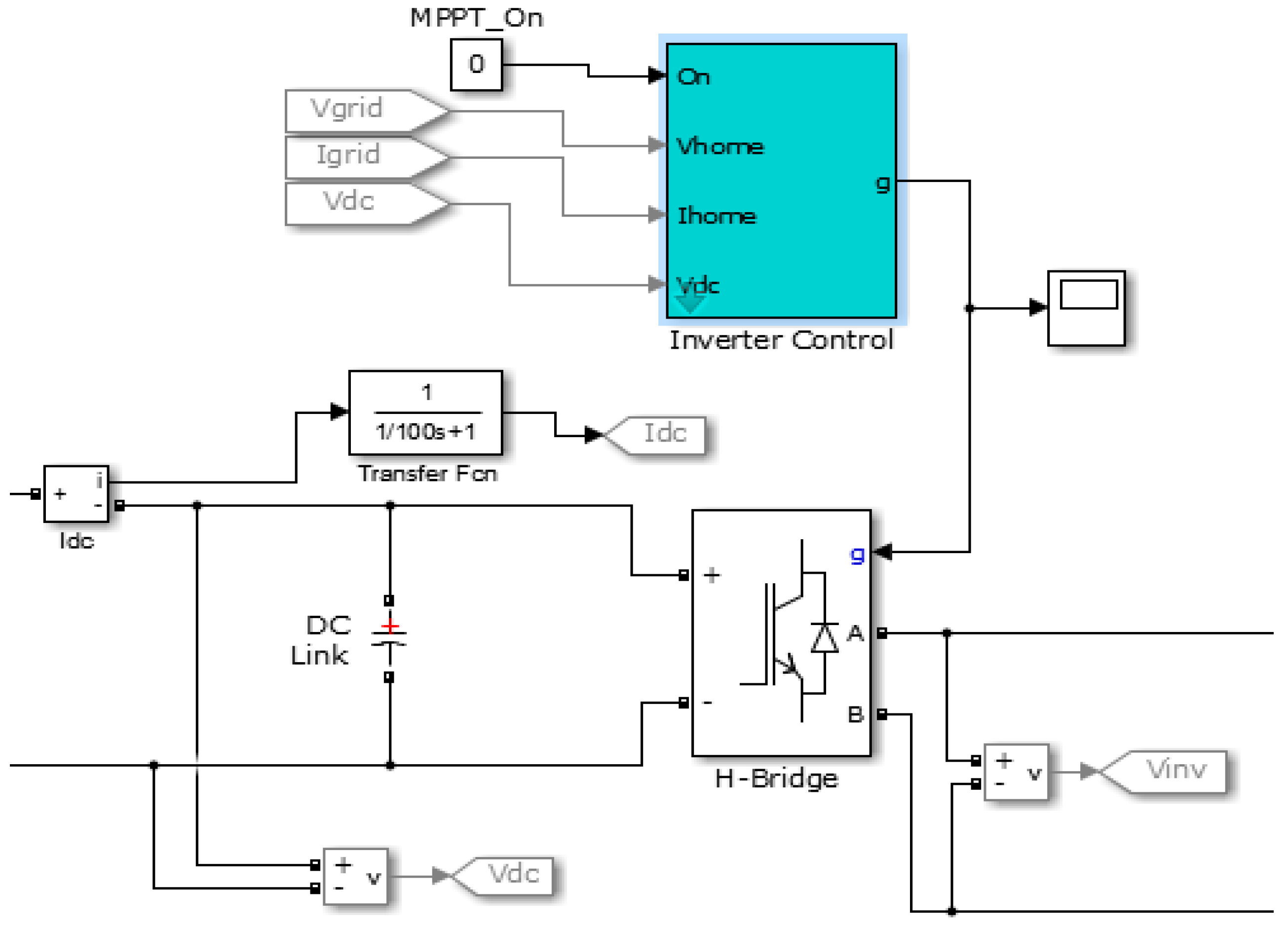
The four-quadrant (4Q) power converter used to rectify the AC voltage uses IGBTs as semiconductors and is controlled through a dedicated PWM controller. The main modifications needed to make it run consisted in disabling the maximum power point tracking (MPPT) system used to extract the maximum power available from the PV panel and adjusting the regulator parameters. This second step has been performed through a trial-and-error method until a functioning device was obtained. A further aspect that has been modified is the value of the DC bus capacitor, which has been changed to 40 mF in order to maintain the voltage ripple in a 5% band. The DC bus nominal voltage has been changed to 500 V from the previous value of 425 V. The new nominal value has been chosen because, actually, it is the maximum voltage that has CHAdeMO and CCS (Combined Charging System).
The converter and its control system are shown in Figure 5. It is necessary to install a DC/DC converter to adjust the current flow to the battery because of the difference between the battery voltage (about 400 V when fully charged) and the main DC bus (500 V). This converter is a two-quadrant converter that allows the power to flow in both directions, i.e., from the battery to the grid or vice-versa.
In this case, the battery charging function is more interesting. The control is done through a PI controller in order to obtain a voltage reference that is able to drive the PWM signal generator. The controller is again tuned through a trial-and-error process. The current reference signal has been made variable so that the regulator is enabled with a current reference equal to zero. The reference signal increases linearly to the maximum value of 250 A in 2 s. Battery, converter and filters are shown in Figure 6.
The connection between the low-voltage systems that supply the power electronics and the medium voltage from the railway line is achieved through a short cable and a power transformer rated at 150 kVA. We decided to maintain the original topology of a centre-tapped two windings transformer used for the 120 V distribution system in the US for a couple of reasons; the most important of those is safety. As both lines are live, but their potential to earth is only 120 V, it is safer for people in case of an insulation failure. We hypothesised a cable of about 200 m length with a cross section of 180 mm2 and a resistance of 0.106 km−1. The transformer and line model is depicted in Figure 7. The resistor Rg represents the Earth system resistance.
The 2 × 25 kV system is modelled as shown in Section 2.2. Four cases have been examined. These are: (a) the absence of trains; (b) the presence of one train; (c) the presence of two trains in the same cells; or (d) the presence of two trains in different cells. This is particularly important, as the main load continues to be the train traffic and the system is viable only if it is possible to power both the railway traffic and the charging facility at the same time. One of the possible scenarios simulated is the presence of two trains in the same cell to evaluate the voltage drop in the system. The considered trains are two modern High Speed Trains with power consumption of 8.8 MW and 9.8 MW, respectively. It is assumed that the two trains absorb a sinusoidal current with a unity power factor. Figure 8 shows the absorbed current by both trains without charging stations connected to the line. It can be seen that the system is capable of supplying both trains with no problem and maintains keeping the line voltage close to its nominal value.
In order to verify that the actual current distribution is comparable to the ideal one, the current at the main transformer and at the autotransformer terminals have been measured (Figure 9). As can be seen, the actual current distribution is close to the ideal one even if some differences due to the real impedances of the line can be noted. In particular, it is possible to observe a small current in the rails and an imbalance between feeder and contact line (catenary).
4. Simulation of the Charging System
The aim of these simulations is to assess how the quality of power of the railway systems is affected by the charging stations for road vehicles. Therefore, the analysis considers simulations of a very detailed model for a short period (max 3.5 s).
There are two simulation steps. The first step is about making the charging system work by itself. It is very important because it allows us to sort out the system problems before the two systems are made to work together. When both systems work as expected, it is then possible to connect them together and have the complete simulation of all the effects.
The first simulation phase has given the following results: the model was working with the following regulator values, 3000 and 1000 as proportional and integrator coefficients for the voltage regulator and 500 and 1000 as proportional and integrator coefficients for the current regulator. The current absorbed was not constant when the device was on full load as the DC bus voltage was still floating. The battery status is shown in Figure 10. It can be seen that the battery is actually recharged from the initial state of charge set to 10%. It shows current and voltage of the battery; current is represented with a negative value because it is charging. On the other end, the battery current would be positive if the battery was discharging. The battery is charged with a constant current using a soft inrush defended by ramp. As the current is constant, the state of charge increases linearly, instead the internal voltage drop is quite proportional to the current in a short time windows; it seems in this period, it is mainly due to the homic voltage drop. Moreover, it is possible to observe the effect of the switching of the power converters in contactors that produce a high-frequency ripple overlap to the main current.
The system is then tested inside the 2 × 25 kV railway line connected between the feeder and the grounding conductor. In this case, the model does not consider only one 100 kW charging spot, but twenty 100 kW charging bays for each direction that cause total power absorption of 4 MW from the railway systems. It is possible to replace the single bay with double bays sharing the same amount of power, thus allowing more people to charge simultaneously even if at a lower rate. The charging area is modelled with one charging bay and a current generator. The idea is to model one charging bay in order to see the current shape it absorbs and, at the same time, inject in the railway system the same current multiplied for the remaining charging bays. The assumption is that all charging bays are working at the same rate. The charging stations are connected from feeder to earth, rather than from catenary to earth, as trains are (Figure 11).
It has been decided to connect the charging facility in the middle of the cell. The first scenario is simulated with no train on the line and the results show that the system works quite well. The simulated time lapse is 3.5 s (Figure 12). In particular, the results are shown towards the end of the simulation because the charger is working at full load there. Figure 9 shows also the impact of all the charging infrastructures installed in two charging areas on the railway voltage. It is possible to remark that the voltage value near the charging area is still inside the limits set for the system on both tracks, despite the fact that the current is not always sinusoidal.
Despite the shape of the current, Figure 13 shows that the autotransformers work as expected by shifting the earth current to the feeder and catenary system. This means that the feeding transformers see the most current coming from the feeder and the catenary with only a small current in the rail as Figure 14 shows. Actually, the two charging areas behave as a low-power HST, and it seems the power requested by the charging infrastructure is about one half of the power requested by a HST during acceleration. In fact, allowed connection between feeder and ground has the same behaviour of the train supplied from contact line and the rails.
The fact that the system works with no trains does not imply that it works while performing its main duty, i.e., powering high-speed trains. In order to verify this, a simulation has been produced in which the system has one or more trains on the tracks. The simulation represents the worst-case scenario with all the loads fed from the two autotransformers.
The first simulation involves the presence of one train on the line. The modelled train is an ETR 400 high-speed train with a maximum power of 9.8 MW located 3 km away from the charging stations. It has been computed that in 3.5 s the train travels less than 500 m, so it has been modelled to assume that the train is still. The total power of the three loads is about 14 MW, so it is expected that the system is able to power all the loads without an excessive voltage drop. The simulation results demonstrate exactly that the three loads can coexist. Figure 15 and Figure 16 show that the voltage measured near the loads and the train is within the limits set by international standards with voltage value being around 23 kV.
There are some differences between this and the preceding scenario; in particular, the currents have a different shape because of the sinusoidal train current superposed to the charger current. Figure 17 and Figure 18 show the currents flowing in the autotransformers and in the main transformer.
The connection of the charging infrastructure between the feeder and the ground attempts to improve the balancing of the system as the current flows directly between the contact line and the feeder without involving the autotransformers and the sells not occupied by the train.
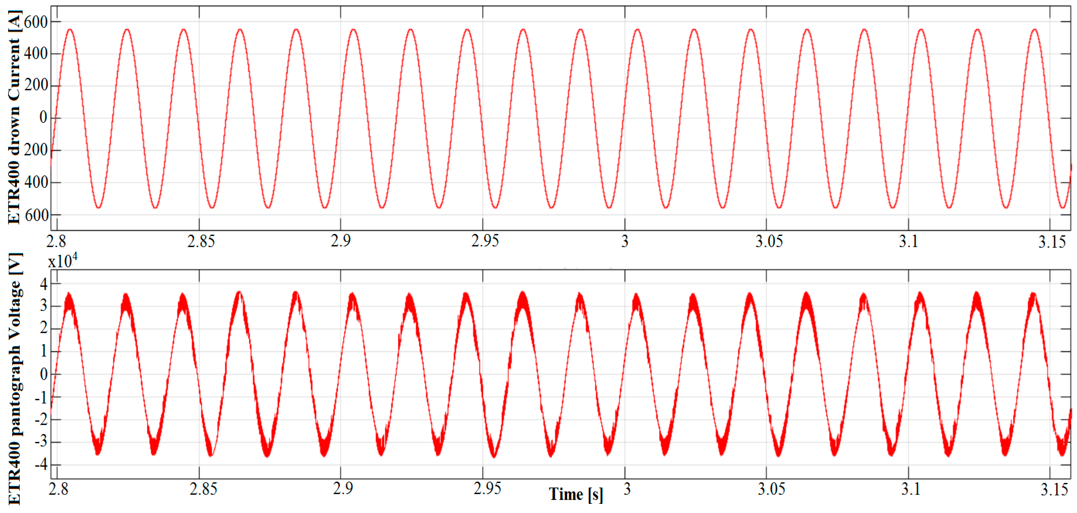
The last scenario evaluates the ability of the system to power two HST at 9.8 MW, each travelling in opposite directions and the same 40 charging bays. This case is very demanding and the system struggles to power the load. This is illustrated by the voltage value, which dropped to about 19 kV as shown in Figure 19 and Figure 20.
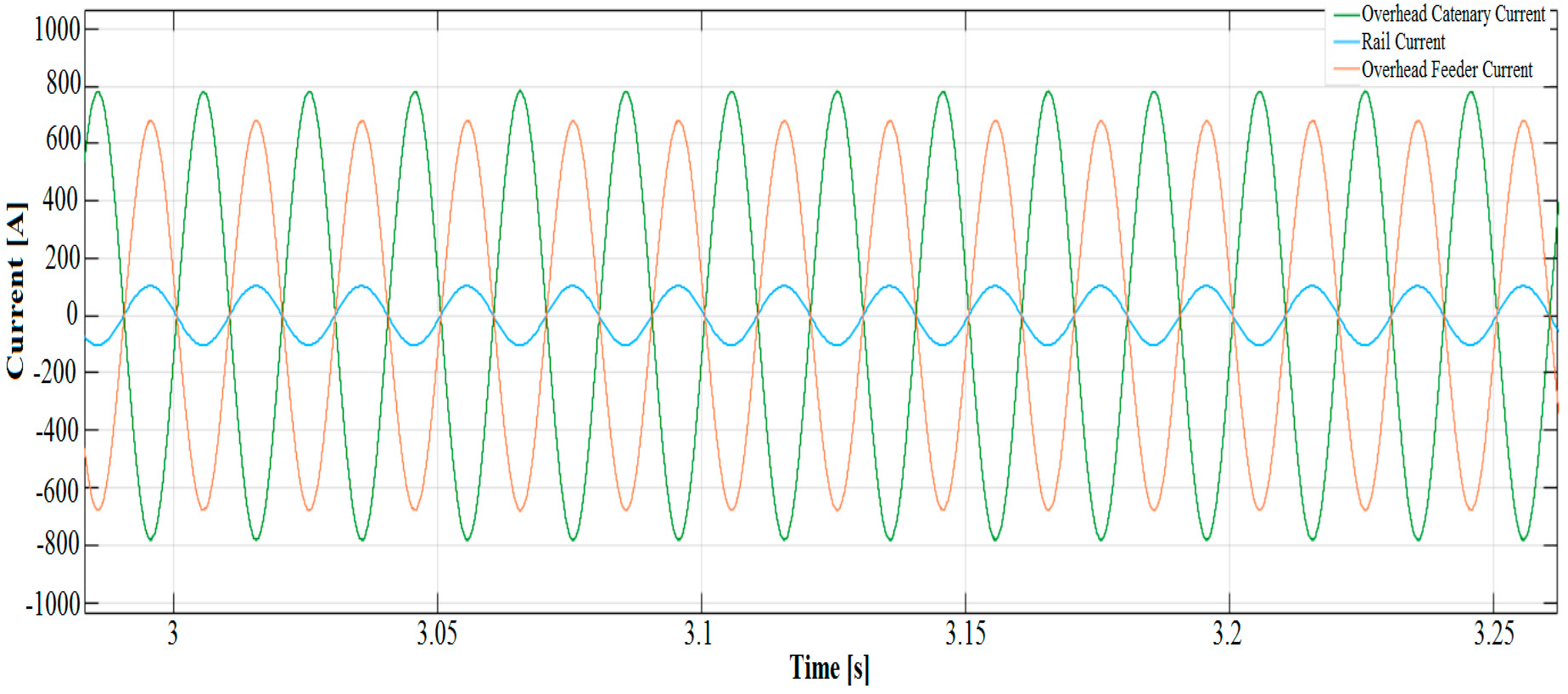
The main similarity with the preceding scenario is that the currents in the feeding transformer and in the autotransformer are significantly influenced by the train rather than the relatively small load given by the charging bays. Figure 21 and Figure 22 depict the current drawn by the autotransformers and the feeding transformer, respectively. The cause of this problem can be traced to two sources: the power converter of battery charging facility or the connection of such a big load between feeder and catenary. It is possible to speculate about the cause of this kind of problem being the connection of such a big load between feeder and earth. The system can cope with the load due to the line technical systems, such as signalling, switches and line diagnostics, but these loads have a maximum rating of 250 kVA each and each substation powers only a few of them.
5. Conclusions
The need to limit pollution enforces stricter emission standards that will increase the cost of producing traditional cars; moreover, increases in oil prices will result in fuel that is more expensive. In the meantime, a reduction in battery costs and government subsidies will lead to an increase in electric vehicle purchases. Another incentive to use electric vehicles comes from both battery manufacturers and the car industry: as battery technology develops further, it will be important to decrease the charging time for the battery pack while maintaining its performance for its entire life expectancy.
As electric vehicles are going to become even more popular, it is necessary to build fast charging infrastructures, especially on the highway network. One of the problems encountered is finding a suitable power source to charge many cars quickly despite the increase in battery capacity and in the number of vehicles in stock. Since the high-voltage grid is not always easily accessible, as the highway lines are usually far from the urban area and from the electricity grid but they are usually close to new high-speed railway lines, the authors have investigated the possibility to supply charging areas from the electric distribution system used for the railway service. These are promising solutions because the power absorbed by the charging areas is of the same order of the magnitude of the power absorbed by the train.
This solution has to compromise the needs of the rail operators, who want their trains adequately powered, and the service areas, who want to offer a service to car drivers.
To demonstrate the feasibility of the concept, a model of a 2 × 25 kV system to feed the railway has been developed. This latter has been implemented in MATLAB/Simulink/SimPower systems to simulate the railway. Then it has been applied to simulate the battery charger and the system.
The results through modelling and simulation disclosed that a compromise is possible but the charging station power has to be limited to allow trains to be properly powered. The simulations reveal that particular attention has to be paid to the quality of the power of the railway system in order to not be compromised by the high-power charging infrastructures. This means that it is not possible to achieve the same refuelling rate of traditional cars because the charging time is much greater than a traditional car refuelling time and the high-speed rail is not able to provide the extra power a larger charging facility needs. Nevertheless, it can be a good solution to begin building the fast charging infrastructure where the high-speed rail is easily accessible.
Author Contributions
Morris Brenna and Michela Longo proposed the core idea, developed the models. They performed the simulations, exported the results and analysed the data. Wahiba Yaïci revised the paper. Morris Brenna, Michela Longo and Wahiba Yaici contributed to the design of the models and the writing of this manuscript.
Conflicts of Interest
The authors declare no conflict of interest.
Nomenclature
| Vi | Negative sequence voltage |
| Vd | Positive sequence voltage |
| Psp | Power of the single-phase load |
| Psc | Three-phase short circuit power of the connection node |
| Umin2 | Lowest non-permanent voltage (max. 10 min) |
| Umin1 | Lowest permanent voltage |
| Un | Normal Voltage 25 kV |
| Umax1 | Highest permanent voltage 27.5 kV |
| Umax2 | Highest non-permanent voltage (max. 5 min) |
| D | Distance between the wires, |
| l | Wire length |
| r0 | Wire radius |
| K | Coefficient representing the current distribution inside the wire |
| ρ | Resistivity of the material, |
| S | Useful cross section of the wire itself |
| [V] | Phasor vectors |
| [I] | Line-to-ground voltage and of the currents flowing in the conductor. |
| Z'ii, Z'ik | values the Carson expressions |
| Rg | Earth system resistance |
References
- Barrero, R.; van Mierlo, J.; Tackoen, X. Energy saving in public transport. IEEE Veh. Technol. Mag. 2008, 3, 26–36. [Google Scholar] [CrossRef]
- Franzitta, V.; Curto, D.; Milone, D.; Trapanese, M. Energy Saving in Public Transport Using Renewable Energy. Sustainability 2017, 9, 106. [Google Scholar] [CrossRef]
- Gunselmann, W. Technologies for increased energy efficiency in railway system. Proc. EPE Power Electron. Appl. 2005. [Google Scholar] [CrossRef]
- Pengling, W.; Xuan, L.; Yuezong, L. Optimization analysis on the energy saving control for trains with adaptive genetic algorithm. In Proceedings of the International Conference on Systems and Informatics (ICSAI), Yantai, China, 19–20 May 2012. [Google Scholar]
- González-Gil, A.; Palacin, R.; Batty, P. Optimal energy management of urban rail systems: Key performance indicators. Energy Convers. Manag. 2015, 90, 289–291. [Google Scholar] [CrossRef]
- Zhang, D.; Zou, F.; Li, S.; Zhou, L. Green Supply Chain Network Design with Economies of Scale and Environmental Concerns. J. Adv. Transp. 2017, 2017, 1–14. [Google Scholar] [CrossRef]
- Mozafar, M.R.; Moradi, M.H.; Amini, M.H. A simultaneous approach for optimal allocation of renewable energy sources and electric vehicle charging stations in smart grids based on improved GA-PSO algorithm. Sustain. Cities Soc. 2017, 32, 627–637. [Google Scholar] [CrossRef]
- Adnan, N.; Nordin, S.M.; Rahman, I.; Amini, M.H. A market modeling review study on predicting Malaysian consumer behavior towards widespread adoption of PHEV/EV. Environ. Sci. Pollut. Res. Int. 2017, 1–21. [Google Scholar] [CrossRef] [PubMed]
- Amini, M.H.; Islam, A. Allocation of electric vehicles’ parking lots in distribution network. In Proceedings of the IEEE PES Innovative Smart Grid Technologies Conference (ISGT), Washington, DC, USA, 19–22 February 2014. [Google Scholar]
- Wang, J.; Wang, C.; Lv, J.; Zhang, Z.; Li, C. Modeling Travel Time Reliability of Road Network Considering Connected Vehicle Guidance Characteristics Indexes. J. Adv. Transp. 2017, 2017, 1–9. [Google Scholar] [CrossRef]
- Bolla, V.; Pendolovska, V. Driving Forces Behind EU-27 Greenhouse Gas Emissions over the Decade 1999–2008; Statistics in Focus 10/2011; Eurostat: Luxembourg, 2011. [Google Scholar]
- Faria, R.; Moura, P.; Delgado, J.; De Almeida, A.T. Managing the Charging of Electrical Vehicles: Impacts on the Electrical Grid and on the Environment. IEEE Intell. Transp. Syst. Mag. 2014, 6, 54–65. [Google Scholar] [CrossRef]
- Wang, X.; Yuen, C.; Hassan, N.U.; An, N.; Wu, W. Electric Vehicle Charging Station Placement for Urban Public Bus Systems. IEEE Trans. Intell. Transp. Syst. 2017, 18, 128–139. [Google Scholar] [CrossRef]
- European Commission. Taking Stock of the Europe 2020 Strategy for Smart, Sustainable and Inclusive Growth. COM (2014) 130 Final. Available online: http://ec.europa.eu/transparency/regdoc/rep/1/2014/EN/1-2014-130-EN-F2-1.Pdf (accessed on 1 August 2017).
- Council Decision 406/2009/EC on the Effort of Member States to Reduce Their Greenhouse Gas Emissions to Meet the Community’s Greenhouse Gas Emission Reduction Commitments Up to 2020. Available online: http://eur-lex.europa.eu/legal-content/EN/TXT/?uri=uriserv:OJ.L_.2009.140.01.0136.01.ENG (accessed on 1 August 2017).
- Hess, A.; Malandrino, F.; Reinhardt, M.B.; Casetti, C.; Hummel, K.A.; Barceló-Ordinas, J.M. Optimal Deployment of Charging Stations for Electric Vehicular Networks. In Proceedings of the UrbaNe’12 First Workshop on Urban Networking, Nice, France, 10 December 2012; pp. 1–6. [Google Scholar]
- Fox, G.H. Electric vehicle charging stations: Are we prepared? IEEE Ind. Appl. Mag. 2013, 19, 32–38. [Google Scholar] [CrossRef]
- Falvo, M.C.; Sbordone, D.; Bayram, I.S.; Devetsikiotis, M. EV charging stations and modes: International standards. In Proceedings of the IEEE International Symposium on Power Electronics, Electrical Drivers, Automation and Motion (SPEEDAM), Ischia, Italy, 18–20 June 2014; pp. 1134–1139. [Google Scholar]
- Baouche, F.; Billot, R.; Trigui, R.; El Faouzi, N.-E. Efficient allocation of electric vehicles charging stations: Optimization model and application to a dense urban network. IEEE Intell. Transp. Syst. Mag. 2014, 6, 33–34. [Google Scholar] [CrossRef]
- Timpner, J.; Wolf, L. Design and evaluation of charging station scheduling strategies for electric vehicles. IEEE Trans. Intell. Transp. Syst. 2014, 15, 579–588. [Google Scholar] [CrossRef]
- Alesiani, F.; Maslekar, N. Optimization of charging stops for fleet of electric vehicles: A genetic approach. IEEE Intell. Transp. Syst. Mag. 2014, 6, 10–21. [Google Scholar] [CrossRef]
- Tesla Supercharger Deployment. Available online: http://www.teslamotors.com/supercharger (accessed on 1 August 2017).
- Rajagopalan, S.; Maitra, A.; Halliwell, J.; Davis, M.; Duvall, M. Fast charging: An in-depth look at market penetration, charging characteristics, and advanced technologies. In Proceedings of the World Electric Symposium and Exhibition (EVS27), Barcelona, Spain, 17–20 November 2013; pp. 1–11. [Google Scholar]
- China National Institute for Standardisation. China’s Standard Proposal Adopted into IEC Standard. July 2014. Available online: http://en.cnis.gov.cn/xwdt/bzhdt/201407/t20140709_19405.shtml (accessed on 1 August 2017).
- Han, Z.; Liu, S.; Gao, S.; Bo, Z. Protection scheme for china high-speed railway. In Proceedings of the 10th IET International Conference on Developments in Power System Protection (DPSP 2010), Managing the Change, Manchester, UK, 29 March–1 April 2010; pp. 1–5. [Google Scholar]
- Kersting, K. Standardization Needs and Testing Methods for Multiple Outlet Chargers. Technical Report. 2014. Available online: http://www.egvi.eu/uploads/IDIADA%20standardisation%20needs%20MOC%20-%20published.pdf (accessed on 1 August 2017).
- CHAdeMO Deployment. Available online: http://www.chademo.com/wp/usmap/ (accessed on 1 August 2017).
- Saponara, S.; Fanucci, L.; Bernardo, F.; Falciani, A. Predictive Diagnosis of High-Power Transformer Faults by Networking Vibration Measuring Nodes with Integrated Signal Processing. IEEE Trans. Instrum. Meas. 2016, 65, 1749–1760. [Google Scholar] [CrossRef]
- Saponara, S. Distributed Measuring System for Predictive Diagnosis of Uninterruptible Power Supplies in Safety-Critical Applications. Energies 2016, 9, 327. [Google Scholar] [CrossRef]
- Ashique, R.H.; Salama, Z.; Abdul Aziz, M.J.B.; Bhattia, A.R. Integrated photovoltaic-grid dc fast charging system for electric vehicle: A review of the architecture and control Renewable and Sustainable. Energy Rev. 2017, 69, 1243–1257. [Google Scholar] [CrossRef]
- Neumann, H.M.; Schär, D.; Baumgartner, F. The potential of photovoltaic carports to cover the energy demand of road passenger transport. Prog. Photovolt. Res. Appl. 2012, 20, 639–649. [Google Scholar] [CrossRef]
- Tulpule, P.J.; Marano, V.; Yurkovich, S.; Rizzoni, G. Economic and environmental impacts of a PV powered workplace parking garage charging station. Appl. Energy 2013, 108, 323–332. [Google Scholar] [CrossRef]
- Bhatti, A.R.; Salam, Z.; Aziz, M.J.B.A.; Yee, K.P. A comprehensive overview of electric vehicle charging using renewable energy. Int. J. Power Electron. Drive Syst. 2016, 7, 114–123. [Google Scholar] [CrossRef]
- Bhatti, A.R.; Salam, Z.; Aziz, M.J.B.A.; Yee, K.P. A critical review of electric vehicle charging using solar photovoltaic. Int. J. Energy Res. 2016, 40, 439–461. [Google Scholar] [CrossRef]
- Yagcitekin, B.; Uzunoglu, M. A double-layer smart charging strategy of electric vehicles taking routing and charge scheduling into account. Appl. Energy 2016, 167, 407–419. [Google Scholar] [CrossRef]
- Mouli, C.; Bauer, G.R.; Zeman, P. System design for a solar powered electric vehicle charging station for workplaces. Appl. Energy 2016, 168, 434–443. [Google Scholar] [CrossRef]
- Morrissey, P.; Weldon, P.; O’Mahony, M. Future standard and fast charging infrastructure planning: An analysis of electric vehicle charging behaviour. Energy Policy 2016, 89, 257–270. [Google Scholar] [CrossRef]
- Wang, Y.; Shi, W.; Wang, B.; Chu, C.-C.; Gadh, R. Optimal operation of stationary and mobile batteries in distribution grids. Appl. Energy 2017, 190, 1289–1301. [Google Scholar] [CrossRef]
- Wang, B.; Wang, Y.; Nazaripouya, H.; Qiu, C.; Chu, C.C.; Gadh, R. Predictive Scheduling Framework for Electric Vehicles With Uncertainties of User Behaviors. IEEE Internet Things J. 2017, 4, 52–63. [Google Scholar] [CrossRef]
- Chen, N.; Gan, L.; Low, S.H.; Wierman, A. Distributional analysis for model predictive deferrable load control. In Proceedings of the IEEE 53rd Annual Conference on Decision and Control (CDC), Los Angeles, CA, USA, 15–17 December 2014; pp. 6433–6438. [Google Scholar]
- Costantino, N.; Serventi, R.; Tinfena, F.; D’Abramo, P.; Chassard, P.; Tisserand, P.; Saponara, S.; Fanucci, L. Design and Test of an HV-CMOS Intelligent Power Switch With Integrated Protections and Self-Diagnostic for Harsh Automotive Applications. IEEE Trans. Ind. Electron. 2011, 58, 2715–2727. [Google Scholar] [CrossRef]
- Saponara, S.; Pasetti, G.; Tinfena, F.; Fanucci, L.; D’Abramo, P. HV-CMOS design and characterization of a smart rotor coil driver for automotive alternators. IEEE Trans. Ind. Electron. 2013, 60, 2309–2317. [Google Scholar] [CrossRef]
- Jensen, T.O.; Danmark, A. High Performance Railway Power Introduction to Autotransformer System (AT). May 2012. Available online: http://www.banekonference.dk/sites/default/files/AT-system%202012.pdf (accessed on 1 August 2017).
- White, R.D. AC 25 kV 50 Hz electrification supply design. In Proceedings of the 4th IET Professional Course on Development Railway Electrification Infrastructure and Systems (REIS), London, UK, 1–5 June 2009; pp. 93–126. [Google Scholar]
- Nardinocchi, A. Electrification and Power Supply. 2011. Available online: http://www.apta.com/mc/hsr/previous/2011/presentations/Presentations/Electrification-and-Power-Supply.pdf (accessed on 1 August 2017).
- Sezi, T.; Menter, F.E. Protection scheme for a new ac railway traction power system. In Proceedings of the IEEE Transmission and Distribution Conference, New Orleans, LA, USA, 11–16 April 1999; Volume 1, pp. 388–393. [Google Scholar]
- Shenoy, J.U.; Sheshadri, K.G.; Parthasarathy, K.; Khincha, H.P.; Thukaram, D. Matlab/psb based modeling and simulation of 25 kV AC railway traction system—A particular reference to loading and fault conditions. In Proceedings of the IEEE Region 10 Conference TENCON, Chiang Mai, Thailand, 24 November 2004; Volume 3, pp. 508–511. [Google Scholar]
- US Department of Energy. Battery Test Results. 2011. Available online: http://media3.ev-tv.me/DOEleaftest.pd (accessed on 1 August 2017).
Figure 1.
Power flow in an ideal 2 × 25 kV autotransformer system.

Figure 2.
Geometry of the conductor’s placement.
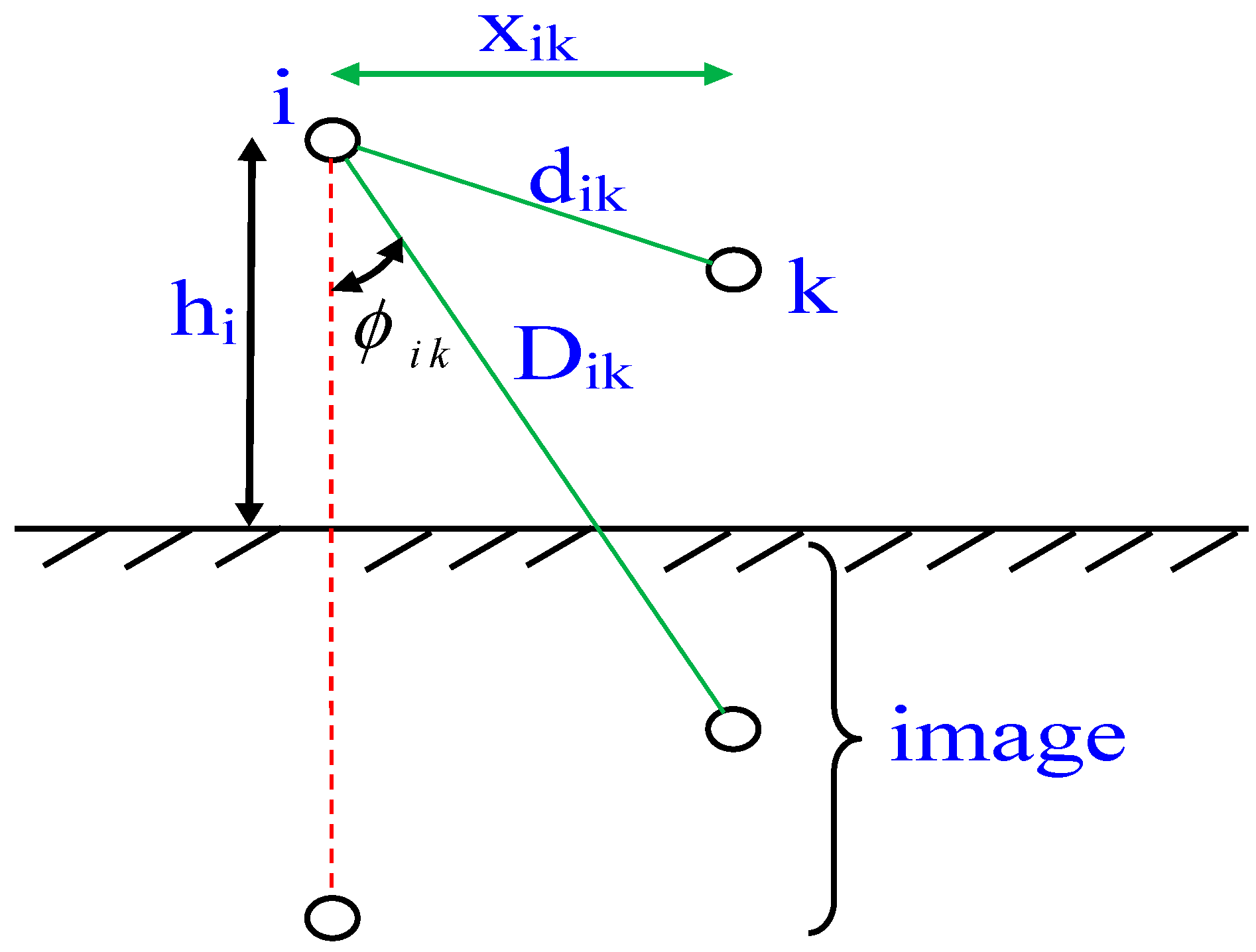
Figure 3.
(a) Two track railway line; (b) Four track railway line.
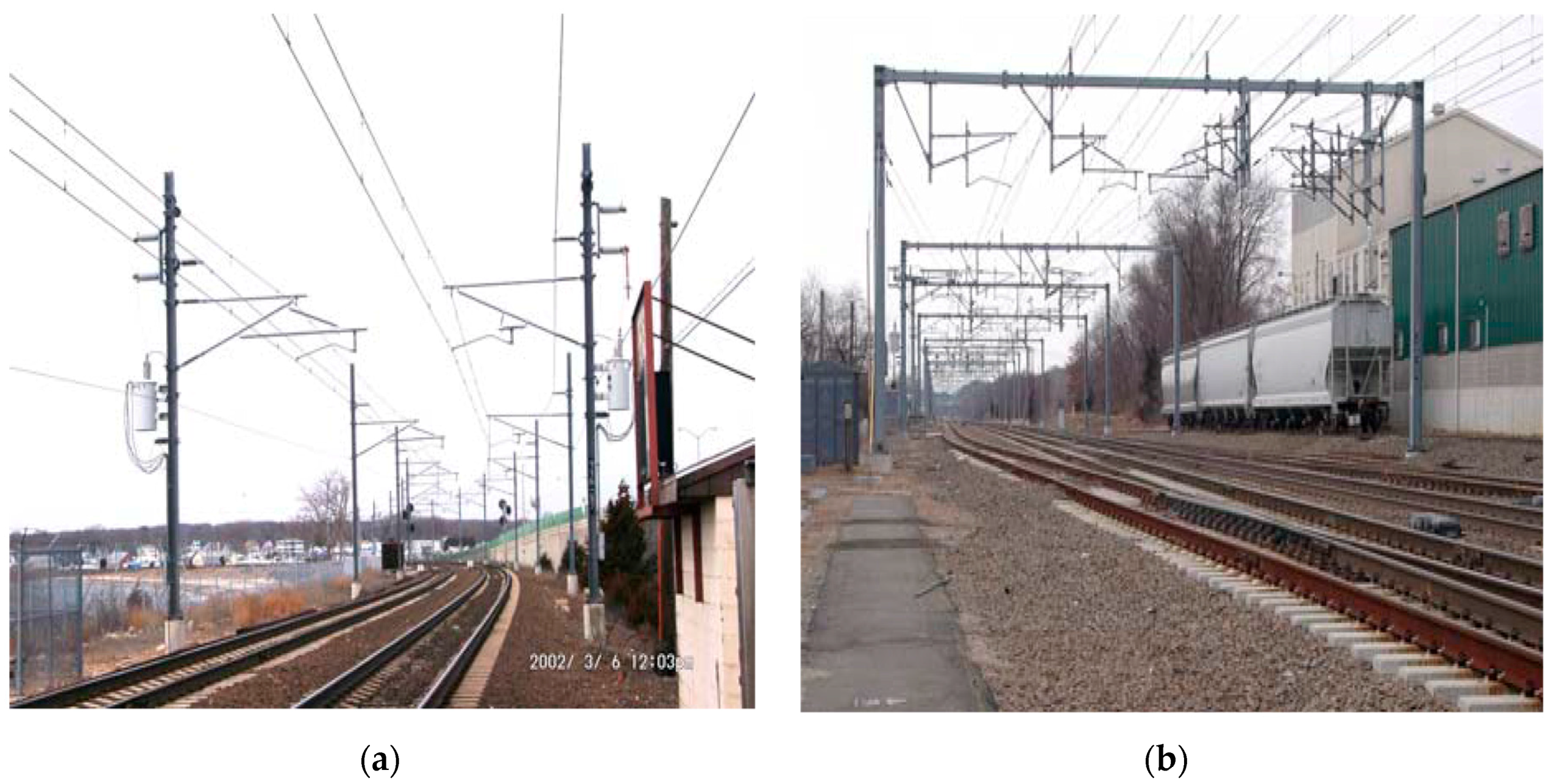
Figure 4.
Electric model of the line including all mutual coupling among live and earthling conductors.
Figure 4.
Electric model of the line including all mutual coupling among live and earthling conductors.
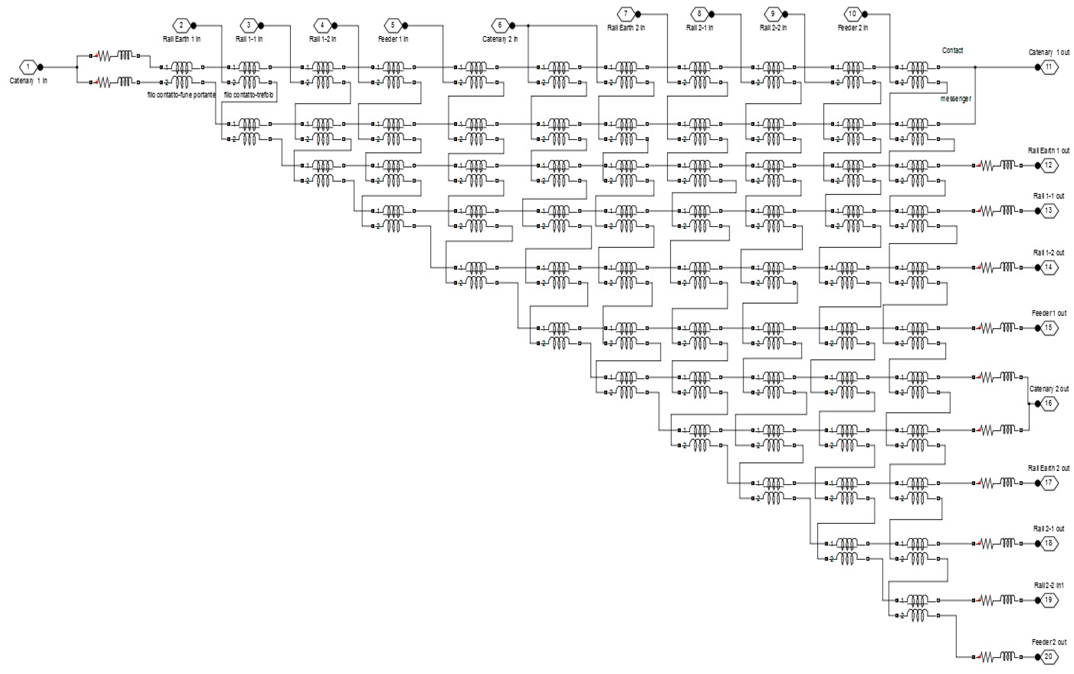
Figure 5.
Model of the four-quadrant (4Q) converter and its control system.

Figure 6.
Model of the car battery and the converter.
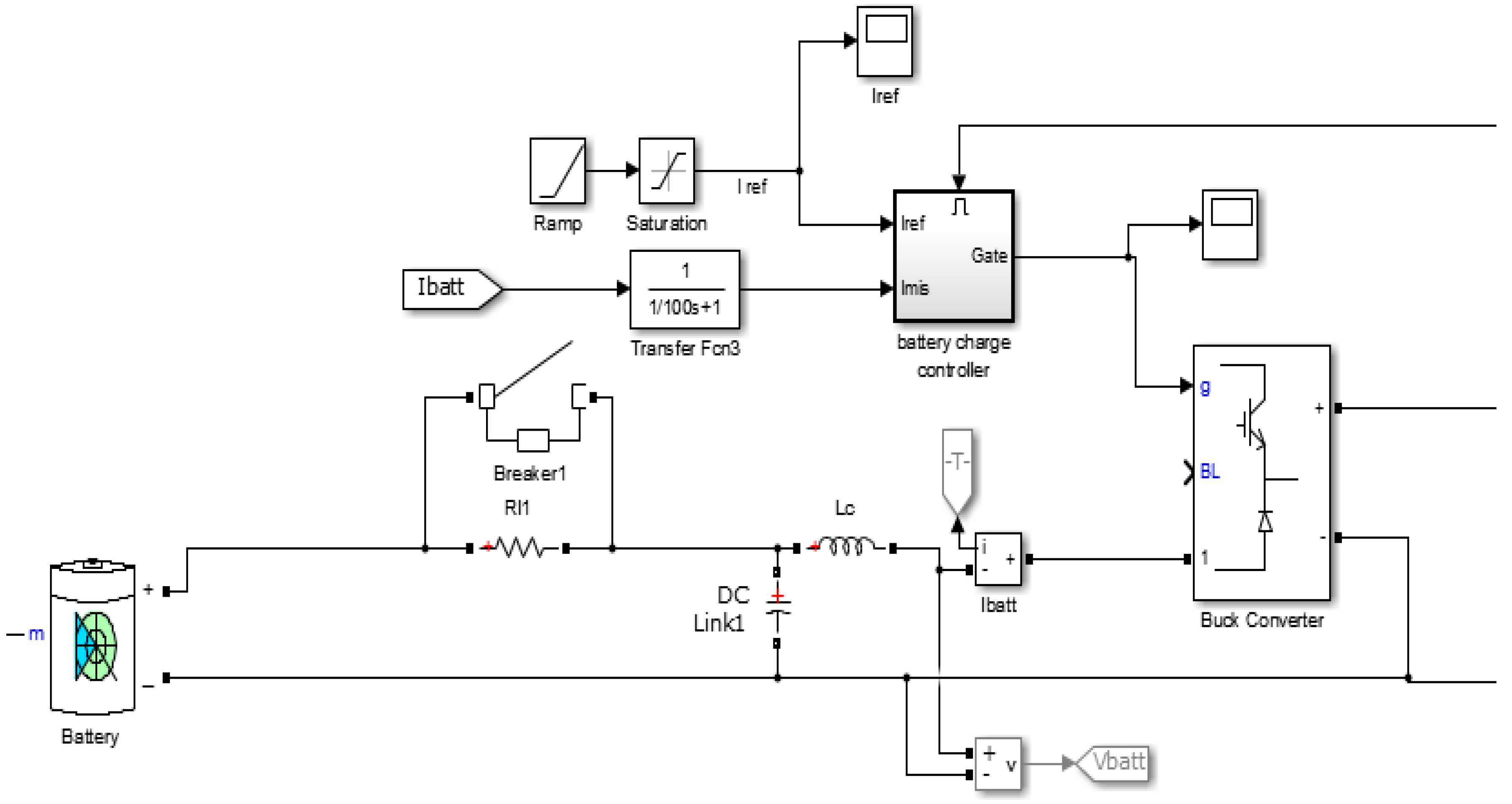
Figure 7.
Model of the power transformer and the short low voltage line.
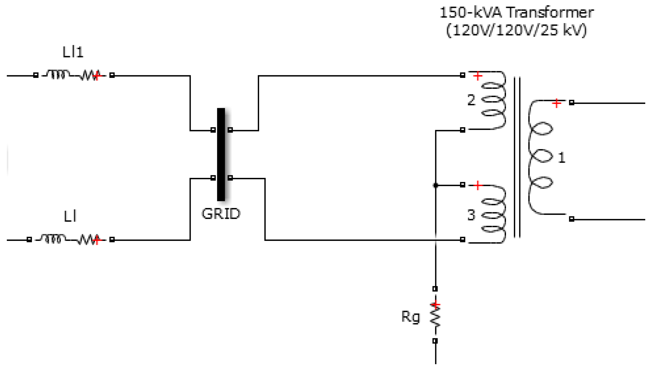
Figure 8.
Voltage and current drawn by a High Speed Train (HST) on a high-speed line with no charging stations.
Figure 8.
Voltage and current drawn by a High Speed Train (HST) on a high-speed line with no charging stations.
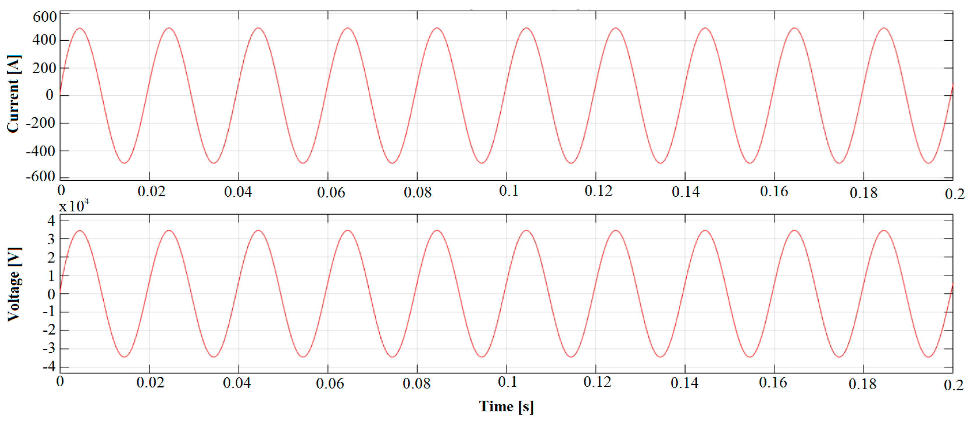
Figure 9.
Currents measured on the (a) feeding transformer connections and (b) autotransformer connections with trains as the only load.
Figure 9.
Currents measured on the (a) feeding transformer connections and (b) autotransformer connections with trains as the only load.
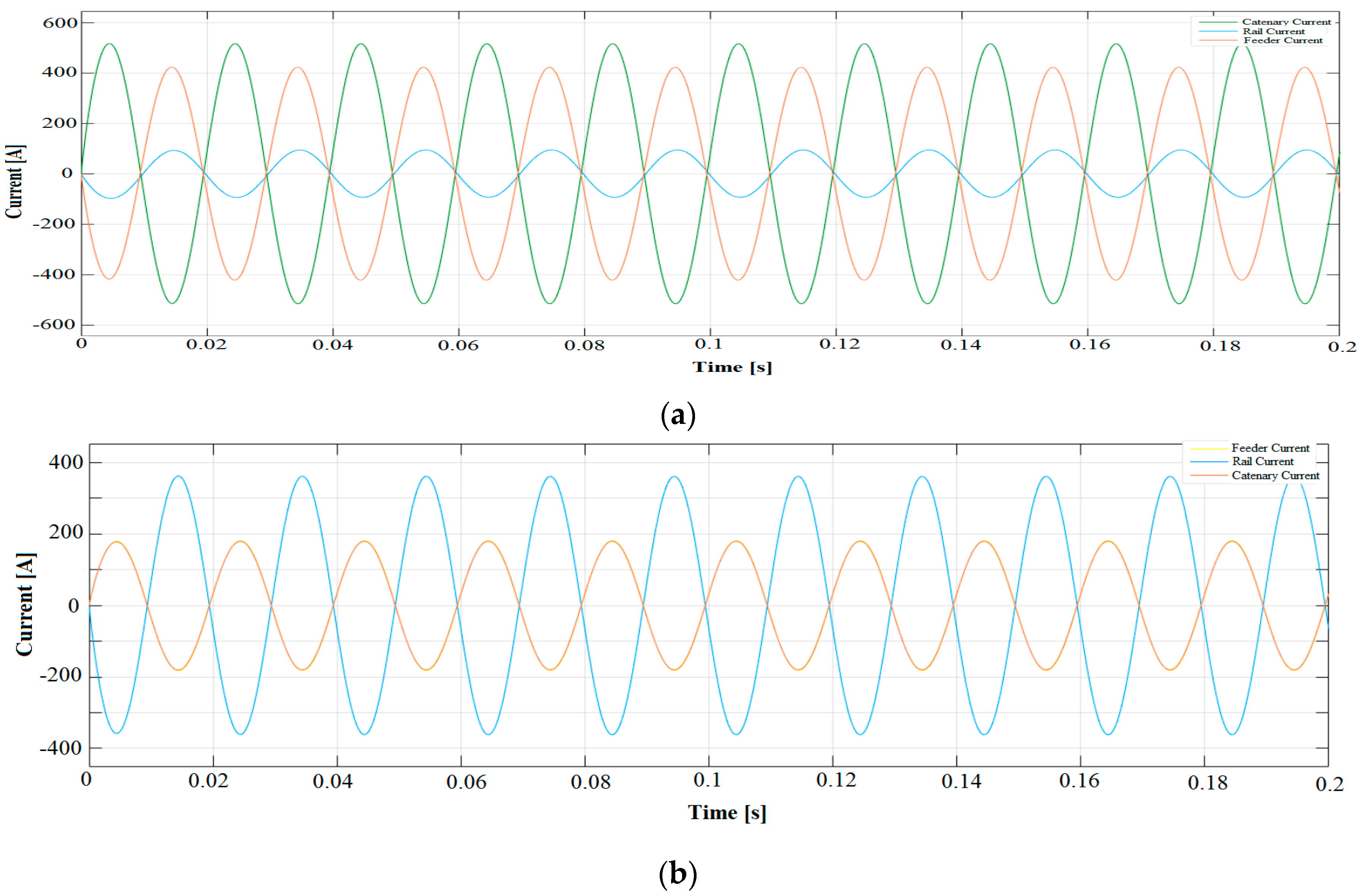
Figure 10.
Battery main variables: state of charge, current and voltage.
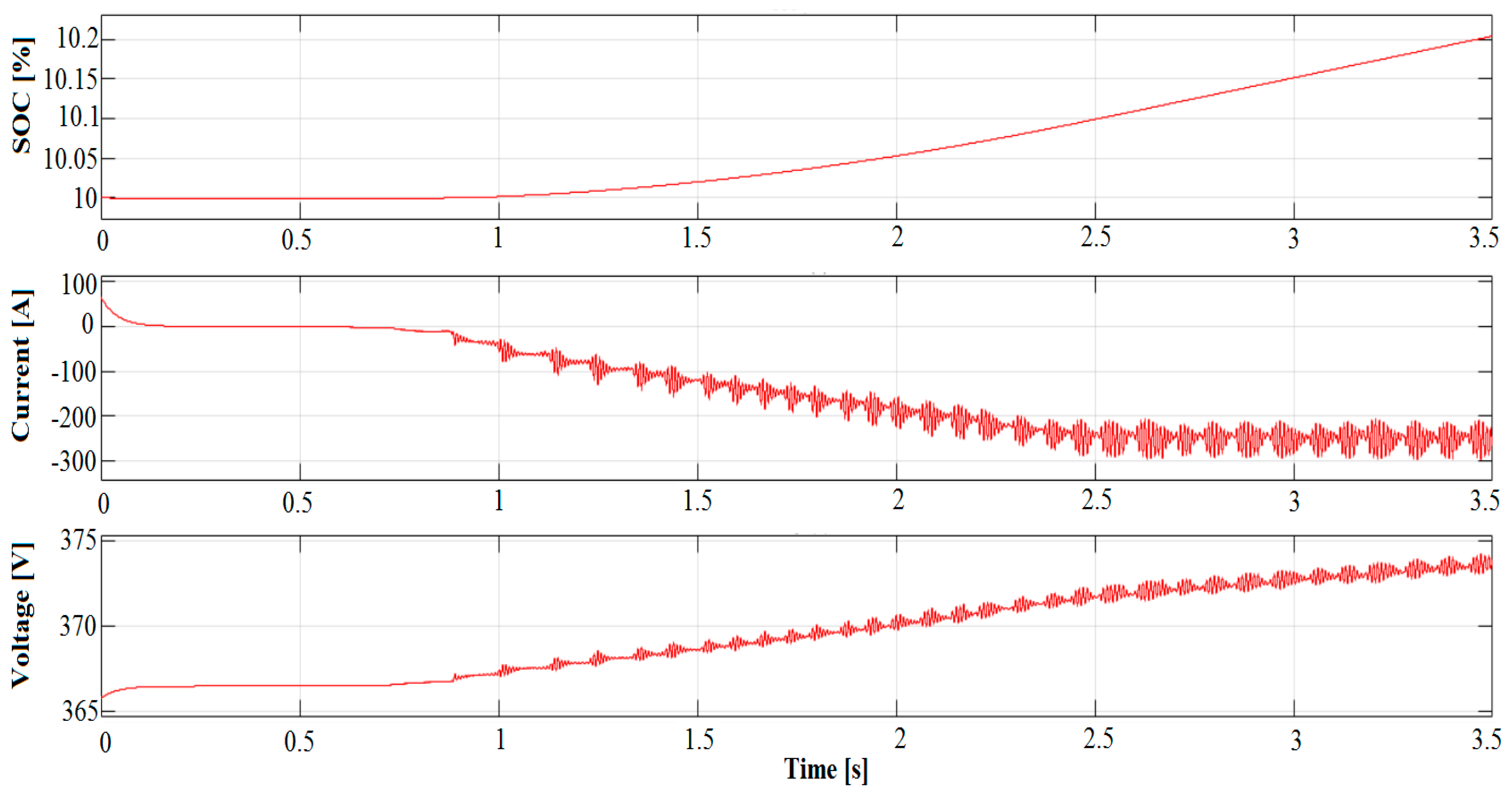
Figure 11.
Section of a real High Voltage (HV) line with indication of the feeder and earth wires.
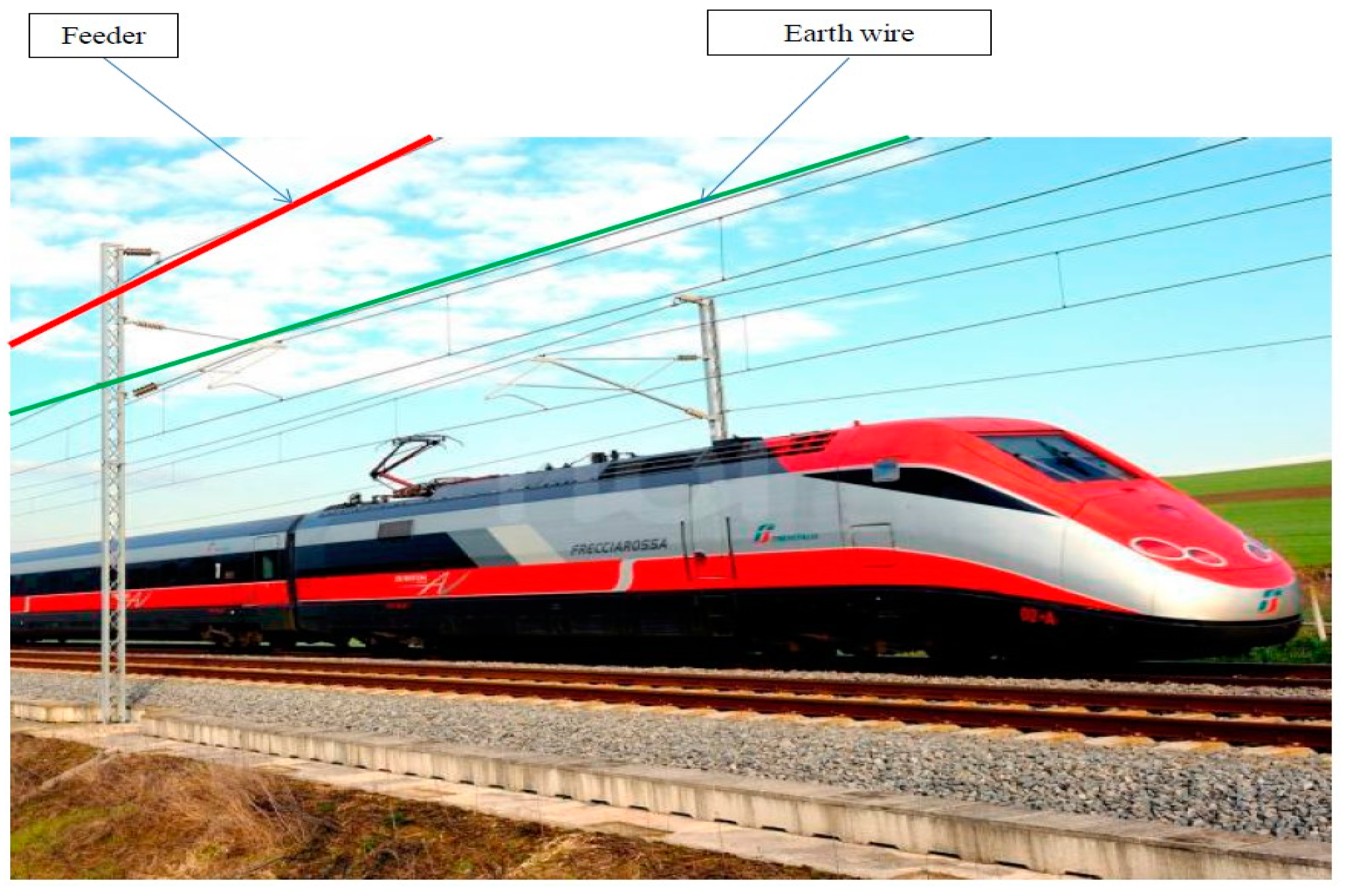
Figure 12.
Feeder and catenary voltage due to the charging station presence.
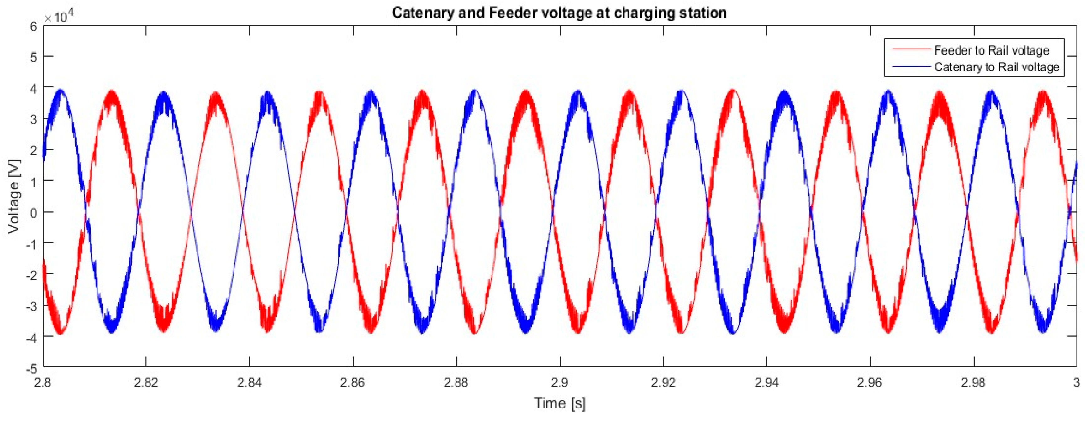
Figure 13.
Current measured on the autotransformers connections due to the charging stations.
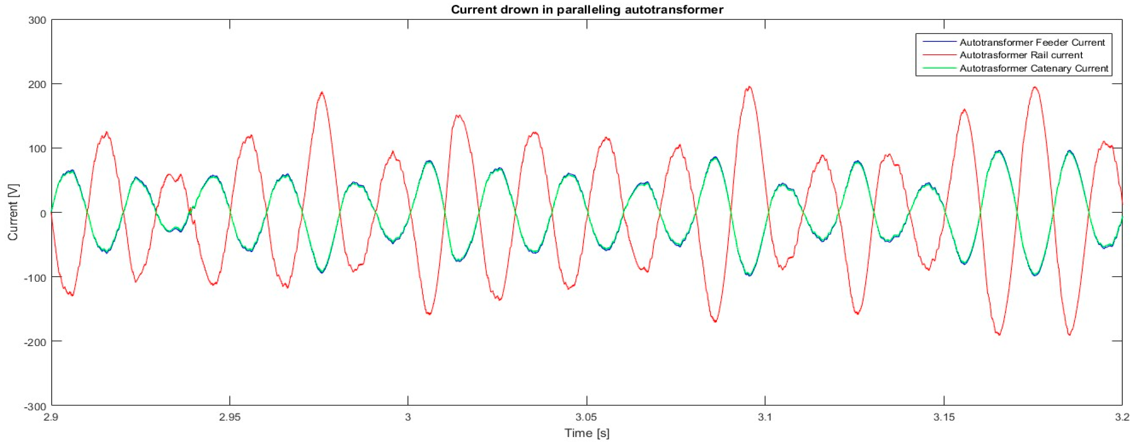
Figure 14.
Current measured on the feeding transformer with the charging stations and no trains on the track.
Figure 14.
Current measured on the feeding transformer with the charging stations and no trains on the track.
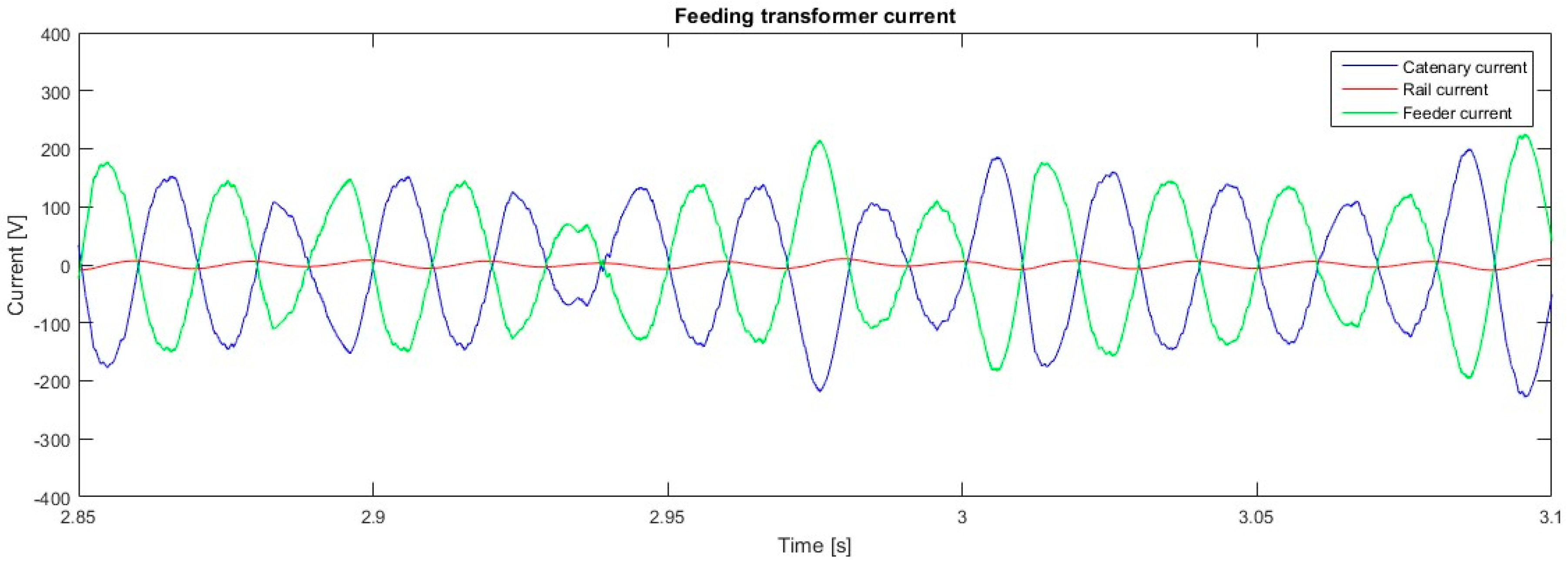
Figure 15.
Catenary and feeder voltages on the charging facility connection point.
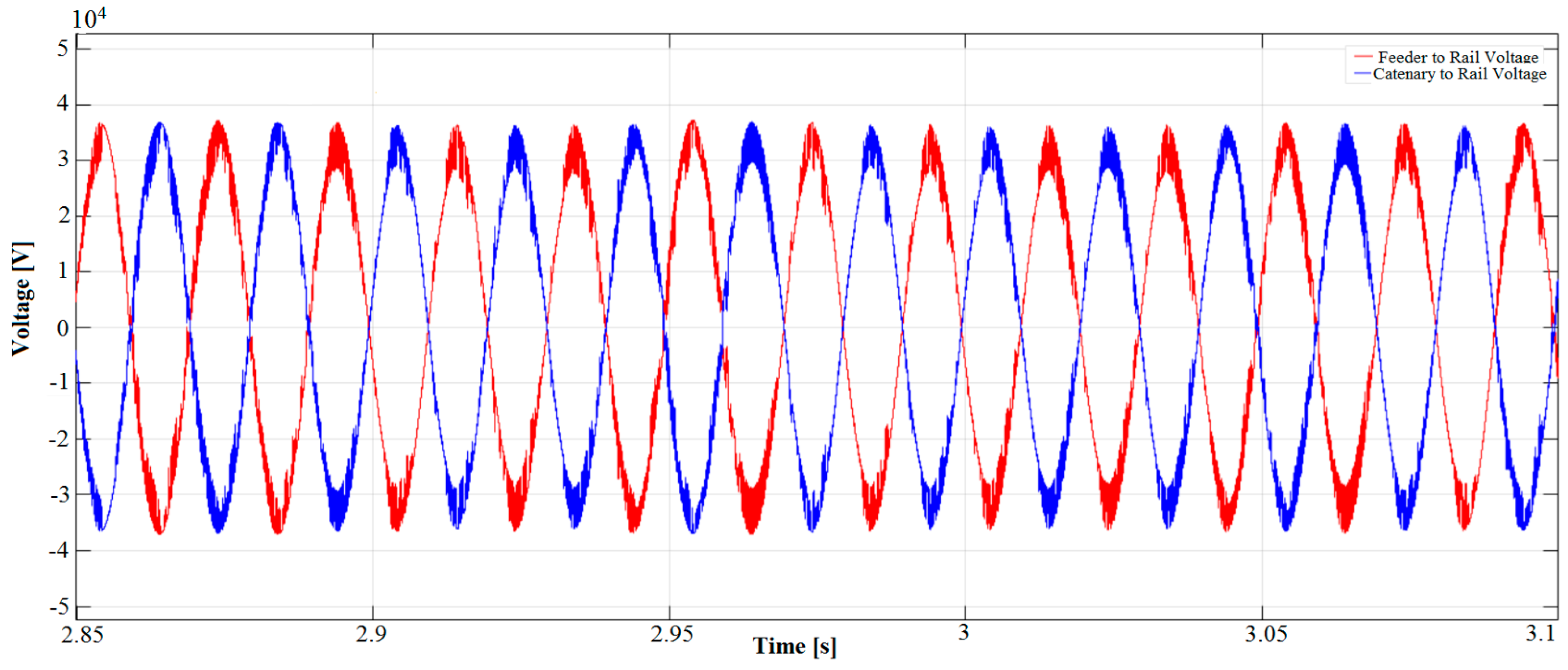
Figure 16.
Voltage on the train position and current drawn by the train.

Figure 17.
Current drawn by the balancing autotransformer with the charging stations and a train on the tracks.
Figure 17.
Current drawn by the balancing autotransformer with the charging stations and a train on the tracks.
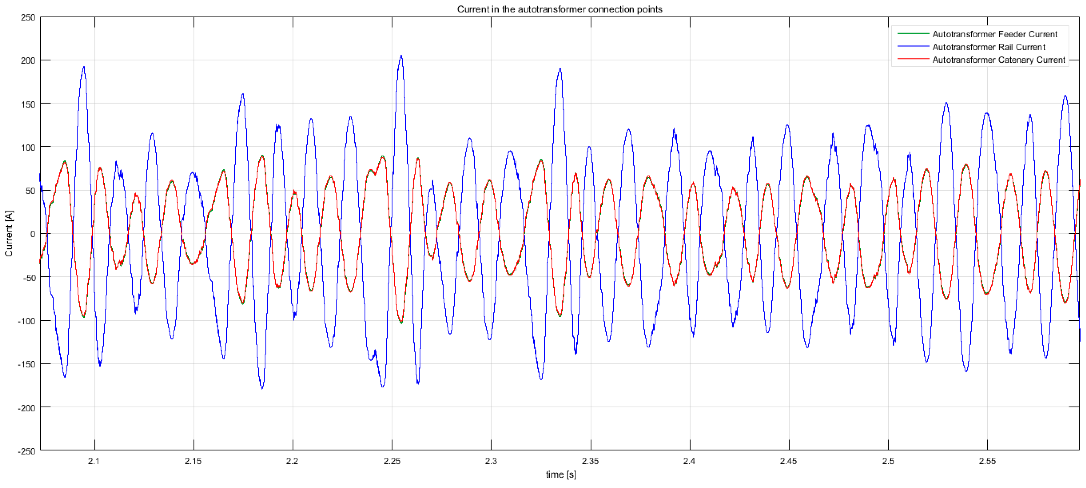
Figure 18.
Current measured on the feeding transformer low voltage winding with the charging stations and a train on the tracks.
Figure 18.
Current measured on the feeding transformer low voltage winding with the charging stations and a train on the tracks.
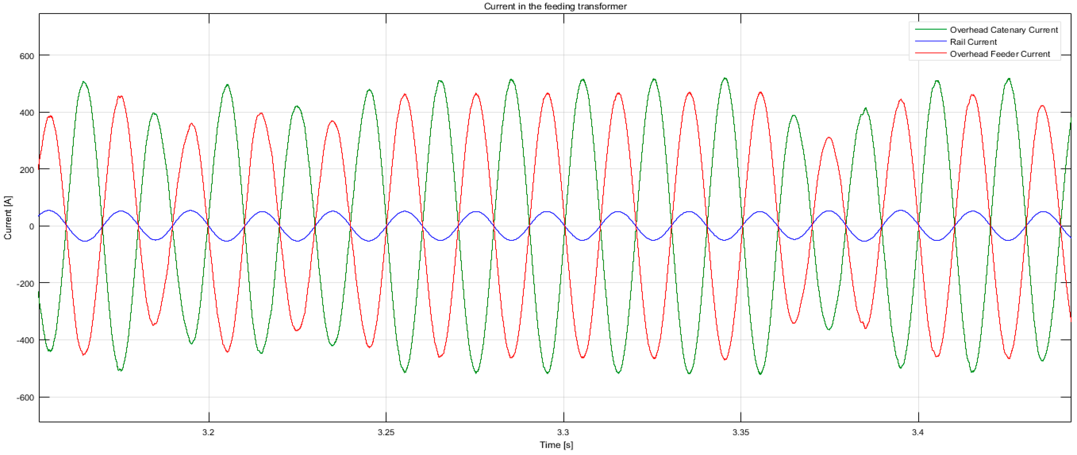
Figure 19.
Voltage on the train position and current drawn by the train with two trains on the track.
Figure 19.
Voltage on the train position and current drawn by the train with two trains on the track.
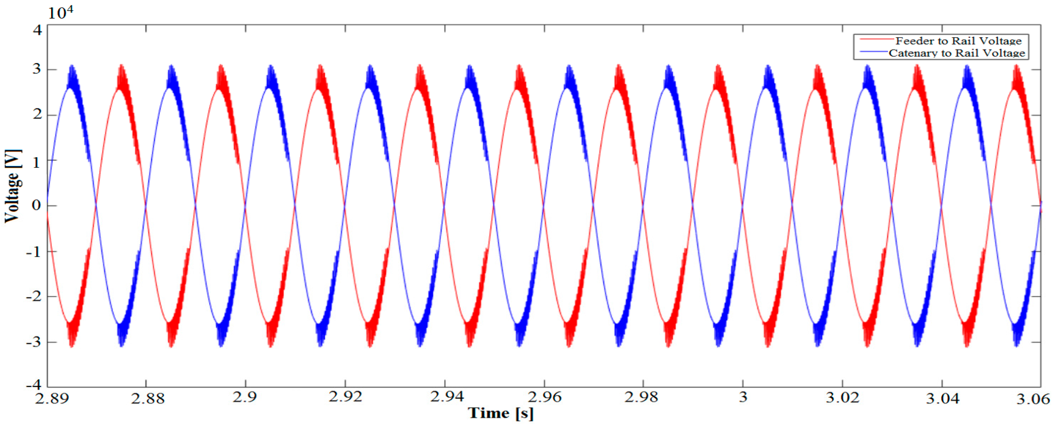
Figure 20.
Voltage at the train pantograph and current drawn.
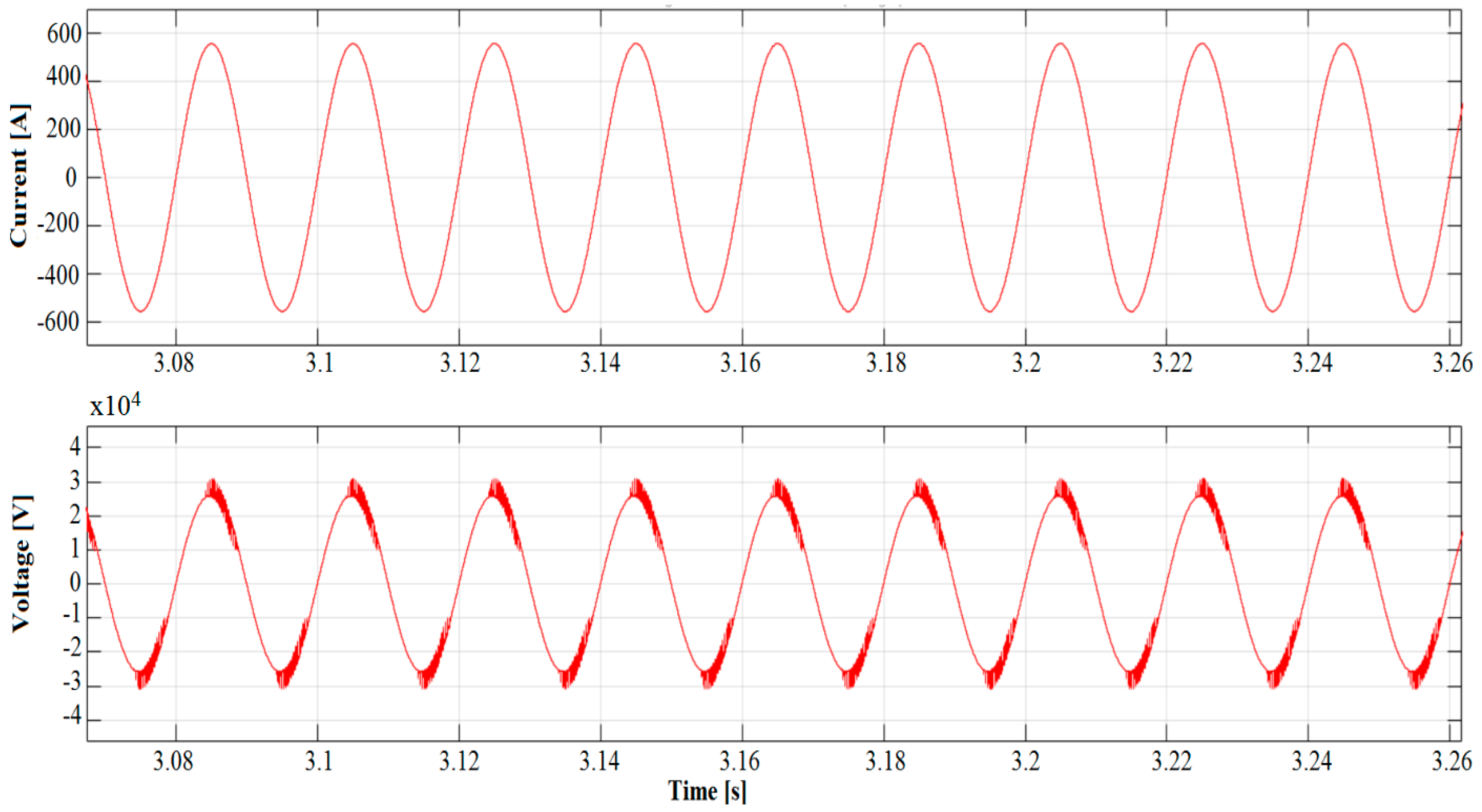
Figure 21.
Current drawn by the autotransformer in the two-train scenario.
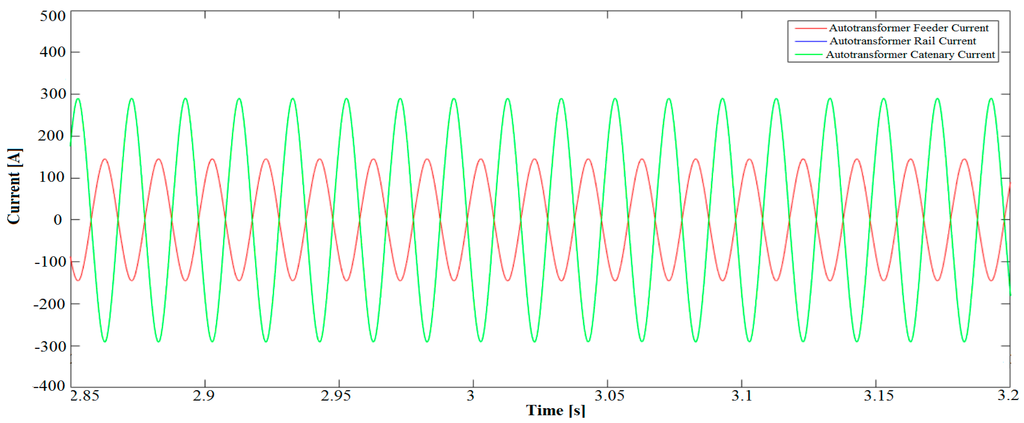
Figure 22.
Current drawn by the feeding transformer in the two-train scenario.


Table 1.
The 25 kV system operating voltages [44].
Table 1.
The 25 kV system operating voltages [44].
| Umin2 | lowest non-permanent voltage (max. 10 min.) | 17.5 kV |
| Umin1 | lowest permanent voltage | 19.0 kV |
| Un | nominal voltage 25 kV | 25.0 kV |
| Umax1 | highest permanent voltage 27.5 kV | 27.5 kV |
| Umax2 | highest non-permanent voltage (max. 5 min.) | 29.0 kV |
Table 2.
Wires and rail positions on an Italian high-speed line built on an embankment.
| Tracks | Wire | X Coordinate (m) | Y Coordinate (m) |
|---|---|---|---|
| Track 1 | Contact wire | −2.5 | 5.3 |
| Messenger wire | −2.5 | 6.55 | |
| Earth wire | −6.1 | 5.5 | |
| Rail 1 | −3.22 | 0 | |
| Rail 2 | −1.78 | 0 | |
| Feeder | −6.6 | 8.0 | |
| Track 2 | Contact wire | 2.5 | 5.3 |
| Messenger wire | 2.5 | 6.55 | |
| Earth wire | 6.1 | 5.5 | |
| Rail 1 | 1.78 | 0 | |
| Rail 2 | 3.22 | 0 | |
| Feeder | 6.6 | 8 |
Table 3.
Main characteristics of the electric vehicle battery.
| Description | Value |
|---|---|
| Nominal voltage (V) | 364.8 |
| Rated pack energy (kWh) | 24 |
| Rated pack capacity (Ah) | 66.2 |
© 2017 by the authors. Licensee MDPI, Basel, Switzerland. This article is an open access article distributed under the terms and conditions of the Creative Commons Attribution (CC BY) license (http://creativecommons.org/licenses/by/4.0/).
Share and Cite
MDPI and ACS Style
Brenna, M.; Longo, M.; Yaïci, W. Modelling and Simulation of Electric Vehicle Fast Charging Stations Driven by High Speed Railway Systems. Energies 2017, 10, 1268. https://doi.org/10.3390/en10091268
AMA Style
Brenna M, Longo M, Yaïci W. Modelling and Simulation of Electric Vehicle Fast Charging Stations Driven by High Speed Railway Systems. Energies. 2017; 10(9):1268. https://doi.org/10.3390/en10091268
Chicago/Turabian StyleBrenna, Morris, Michela Longo, and Wahiba Yaïci. 2017. "Modelling and Simulation of Electric Vehicle Fast Charging Stations Driven by High Speed Railway Systems" Energies 10, no. 9: 1268. https://doi.org/10.3390/en10091268
Note that from the first issue of 2016, this journal uses article numbers instead of page numbers. See further details here.