
A Principal Components Rearrangement Method for Feature Representation and Its Application to the Fault Diagnosis of CHMI


1
Department of Electrical Automation, Shanghai Maritime University, Shanghai 201306, China
2
Institut d’Electronique et Télécommunications de Rennes, UMR CNRS 6164, Polytech Nantes, Rue Christian Pauc, BP 50609, 44306 Nantes CEDEX 3, France
*
Author to whom correspondence should be addressed.
Energies 2017, 10(9), 1273; https://doi.org/10.3390/en10091273
Submission received: 26 July 2017
/
Revised: 20 August 2017
/
Accepted: 24 August 2017
/
Published: 26 August 2017
(This article belongs to the Section I: Energy Fundamentals and Conversion)
Abstract
:Cascaded H-bridge Multilevel Inverter (CHMI) is widely used in industrial applications thanks to its many advantages. However, the reliability of a CHMI is decreased with the increase of its levels. Fault diagnosis techniques play a key role in ensuring the reliability of a CHMI. The performance of a fault diagnosis method depends on the characteristics of the extracted features. In practice, some extracted features may be very similar to ensure a good diagnosis performance at some H-bridges of CHMI. The situation becomes even worse in the presence of noise. To fix these problems, in this paper, signal denoising and data preprocessing techniques are firstly developed. Then, a Principal Components Rearrangement method (PCR) is proposed to represent the different features sufficiently distinct from each other. Finally, a PCR-based fault diagnosis strategy is designed. The performance of the proposed strategy is compared with other fault diagnosis strategies, based on a 7-level CHMI hardware platform.
1. Introduction
Due to the limitation of natural resources and increased pollution caused by fossil fuels and nuclear power, renewable energy research has become a hotspot [1]. As an important part of energy conversion, cascaded H-bridge Multilevel Inverter (CHMI) is widely used in high power applications for medium and high voltages thanks to its high switching frequency, small number of components and low total harmonic distortion [2,3,4]. However, when its level increases, the reliability of the inverter will be reduced due to the eventual loss and faults of components [5,6]. The healthy functioning of an inverter plays an important role in the process of DC to AC power conversion [7]. Therefore, the fault diagnosis of CHMI is particularly important [8,9,10].
To achieve a good fault diagnosis, it is crucial to extract representative and distinctive fault features [11]. Principal Component Analysis (PCA) is an efficient tool to extract useful features, especially from high-dimensional data [12], such as the fault data of CHMI. Recently, lots of PCA-based feature extraction methods have been proposed for fault diagnosis of CHMI. In [13], after the Fourier transform of data, the dimension of fault features is reduced by PCA. In [14], PCA is used to reduce the input data of Back Propagation Neural Network (BPNN). However, considering the unavoidable noise and high-dimension of large data, if the classical PCA is used only, the fault features may not be sufficiently distinct from each other due to the great similarity between several signals among different categories in CHMI. When perturbed by noise, the similarity degree of features may become too big to ensure the performance of fault diagnosis. As a result, improved PCA algorithms have been proposed for the fault diagnosis of CHMI. For example, Ref. [15] has adopted Relative Principal Component Analysis (RPCA) for feature rearrangement of the fault data acquired from CHMI. Ref. [16] has used Kernel Principal Component Analysis (KPCA) for feature extraction and fault detection of high-voltage circuit breakers. Though the improved PCA algorithms are able to extract more useful information of high-dimensional data, this improvement is made before the steps of the PCA algorithm, which has some inherent drawbacks, such as the great complexity due to the selection of the relevant relative information of Principal Components (PCs) [17,18], the big similarity [19,20,21] between some features corresponding to different fault categories after utilizing the PCA method, etc.
The main problem is that the different fault features extracted by PCA are affected by noise and may be very similar to ensure a good performance in fault diagnosis of CHMI. Therefore, signal denoising and data preprocessing are necessary before feature extraction. Principal Components Rearrangement (PCR), a feature representation method, is proposed in this work. This method tries to make the features extracted by PCA sufficiently distinct to facilitate their diagnosis. PCR consists of three parts: the PCA-based feature extraction, features rearrangement of each PC and new projection matrix rebuilding.
The rest of this paper is organized as follows. Section 2 describes a common problem of CHMI with a resistive load of finite value. Section 3 details the steps of the proposed PCR method. In Section 4, a PCR-based fault diagnosis strategy is presented. In Section 5, the performance of the proposed PCR-based fault diagnosis strategy is verified and compared with other related fault diagnosis strategies, based on a 7-level CHMI hardware platform. Finally, Section 6 concludes the paper.
2. Problem Description
In this section, firstly, the useful signals are selected for the fault diagnosis of CHMI. Then, the structure of the original data is described. Finally, a common problem of CHMI with a resistive load of finite value is described.
2.1. Fault Signal Analysis
The acquisition of effective signals plays an important role in the fault diagnosis of CMHI. In this paper, the voltage signals are chosen as the signals for the fault diagnosis, and Open Circuit (OC) of switching devices in CHMI is considered as the fault cause. The analysis is as follows.
When a fault occurs at any switch, the voltage and current signals will be unbalanced and distorted. Voltage and current are the main signals allowing to make the fault diagnosis of CHMI [22]. Compared with the voltage signals, the load has greater effects on the current signals, which are not suitable for the fault diagnosis [22]. Moreover, when there exist logic errors of driving signals, under-voltage of power supply, over-voltage breakdown, avalanche breakdown and thermal breakdown, etc., Short Circuit (SC) may occur at switching devices of CHMI. Because the time of SC is very short (nomally within 10 s), usually, it is too late to diagnose a SC due to its great destruction to CHMI, which may make the system break down promptly and sometimes even irreversibly. As a result, the SC protection of switching devices is always based on hardware such as protection circuits, usually the fuses. Then, SC can be converted to OC. Therefore, both SC and OC, two main faults of switching devices of CHMI, can be attributed to OC for fault diagnosis [23]. Consequently, the voltage signals of OC are selected for fault diagnosis of CHMI.
The topology of a CHMI is shown in Figure 1, where m represents the number of H-bridges. The last H-bridge is denoted as “H_bottom”. The labels of different conditions are shown in Table 1 according to the notations in Figure 1. For example, there are 12 single switch faults plus the normal condition when m3, giving a total of 13 different situations. Figure 2 shows the voltage signals for a 7-level CHMI without load, which means that the value of load is infinite. We can observe that when an OC occurs at H-bridge 1, Switch 1 (HS) at 0.02 s, the voltage amplitude is decreased from 72 V to 48 V. When OC occurs at other switching devices, the changes of voltage amplitudes are all obvious and different from each other as circled in Figure 2. Therefore, the amplitudes of OC voltage signals can be used as the features for fault diagnosis of CHMI.
2.2. Structure of the Original Data
The structure of the original acquired data for fault diagnosis is described in Figure 3. There are I categories (normal and fault situations), J observations for each category and N sampling points with each observation. The total observations are MI × J. Consequently, the original data can be represented by a matrix of dimension (M, N). After the original data are denoised or preprocessed, the structure of the processed data remains the same.
2.3. Problem Description in CHMI
When an OC occurs in CHMI, even the load has less effects on the voltage signals than the current signals, and these effects can’t be ignored. The resulting voltage signals in CHMI with a resistive load of finite value may become very similar. For illustrating the problem, a 7-level CHMI with a load of finite value is used.
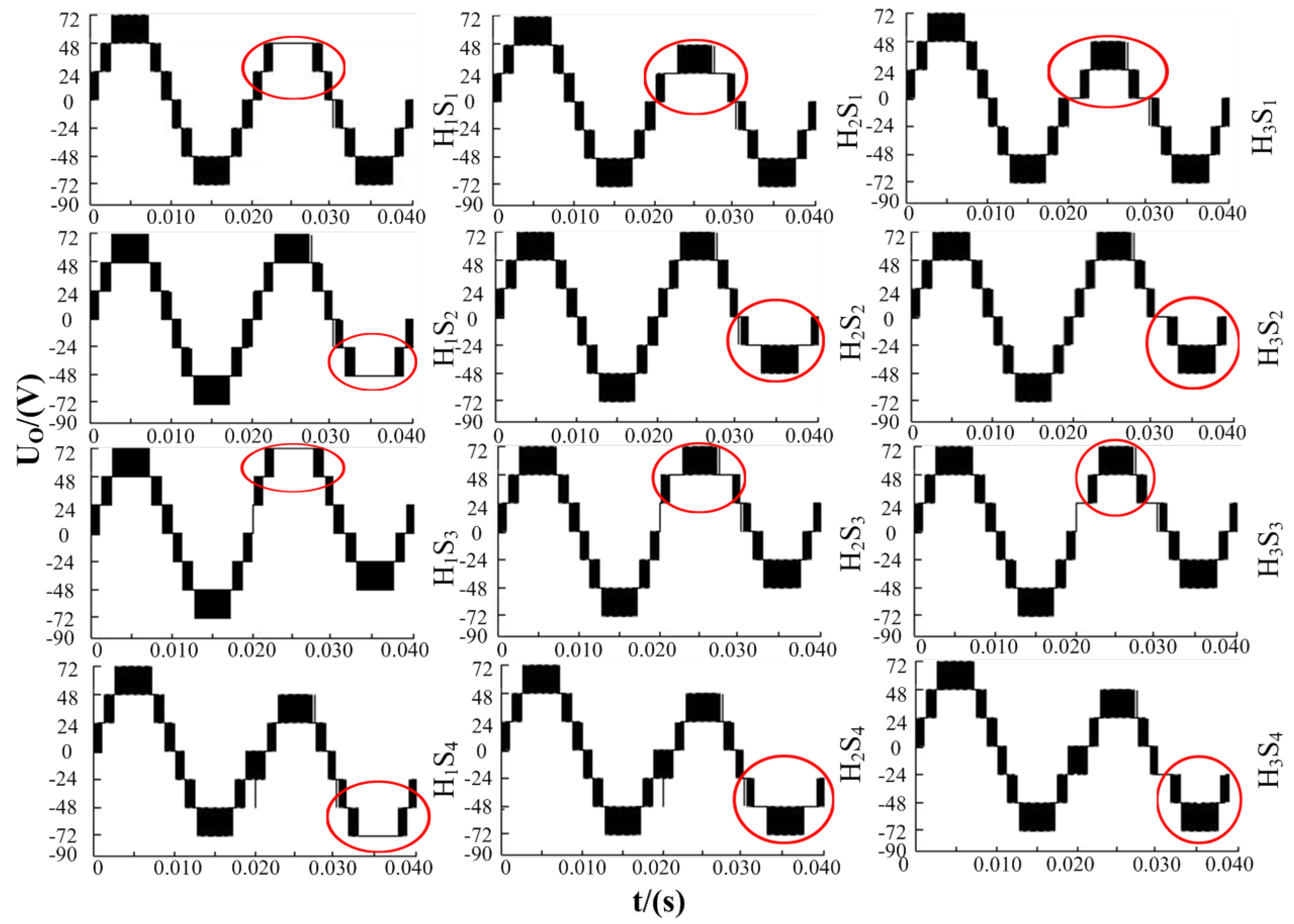
To give a practical example of similar fault signals, a resistive load is used in CHMI. Here, 5 is used in the 7-level CHMI model to describe the problem in CHMI. The resulting voltage signals are shown in Figure 4. The voltage signals are different for different faults except for H, the last H-bridge. When an OC occurs, the signals are very similar (almost the same) at the cross positions (HS, HS and HS, HS), which will make their diagnosis very difficult.
As shown in Figure 5, the problem remains the same at the cross positions in H_bottom of CHMI when m is set as 4, 5 and 6 corresponding to level-9, level-11 and level-13 of CHMI, respectively. Therefore, the problem that the voltage signals are very similar at the cross positions in H_bottom of CHMI can not be avoided, and this common problem will influence the performance of the final fault diagnosis. Additionally, affected by noise during the data acquisition, the fault diagnostic performance will be worse.
To overcome the above problems, after the necessary signal denoising and data preprocessing, an effective feature representation method and a fault diagnosis strategy are proposed in this paper.
3. PCR Method
For fixing the problem of great similarity between some features, the PCR method is proposed in this paper. This section provides details of this method, which includes the PCA-based feature extraction, features rearrangement of each PC and new projection matrix rebuilding.
3.1. PCA-Based Feature Extraction
PCA is usually used to reduce the dimension of data and extract useful features. The steps of the classical PCA method [24] are described as follows.
Let be a M × N real data matrix, where M, N represent the number of total observations and the number of sampling points in each observation, respectively. MIJ , where I, J are, respectively, the number of categories and the number of each category’s observations.
Firstly, X is normalized by Equation (1) for numerical efficiency without any physical meanings:
The correlation matrix of can be estimated by [25]:
Let and , where i = 1, 2,…, I, be its eigenvalues and the corresponding eigenvectors respectively. The Cumulative Percentage of Variance (CPV) is defined as:
Denote the projection matrix of PCA by , which is constituted by the eigenvectors corresponding to the k largest eigenvalues. The resulted data after dimension reduction are given by:
which can be specified as:
Each column of Y is a PC, which is used as the input data for the rearrangement method described as follows.
3.2. Features Rearrangement of Each PC
This part describes the rearrangement method in order to make the features of each PC sufficiently distinct. The features rearrangement of each PC includes the two following steps.
Step 1: Selection of one column of
The selected cth column of can be written as:
where . Considering the I categories, can be rewritten as
There are J observations in each category. Thus, belongs to the ith category in vector , where .
Step 2: Features rearrangement for each PC
Denote the vector of mean values of I categories by:
where the mean value of the ith category is calculated by . Let the data interval length of be , given by:
In order to make the different categories sufficiently distinct, a straightforward and easy way is to make the length of different categories equal to the maximum data interval length, which is defined as:
For the ith category of , can be rearranged as:
where and is the lth largest value in . Finally, the cth PC vector after the rearrangement is given by:
3.3. New Projection Matrix Rebuilding
When all the k PC vectors are rearranged, the final rearranged matrix can be written as:
According to the data matrix and the rearranged data matrix (14), the new projection matrix can be built to replace the initial projection matrix (5) as:
where represents the pseudoinverse of X, which can be obtained through the following Singular Value Decomposition (SVD) of X:
where , and I is an identity matrix. Then, can be calculated as:
where the diagonal matrix is obtained by inversing all the diagonal elements having value greater than of the diagonal matrix S.
4. Fault Diagnosis Strategy Based on PCR
As shown in Figure 6, a fault diagnosis and tolerant control system usually contains six steps: signal denoising, data preprocessing, feature representation, fault classification, diagnosis results output and fault-tolerant control. Focusing on the first four steps, this section details a PCR-based fault diagnosis strategy.
4.1. DWT-Based Signal Denoising
Noise affects the success of fault detection and classification. Denoising the measured signals plays a vital role in effective fault diagnosis. For this purpose, Discrete Wavelet Transform (DWT) by using multiscale wavelet decomposition and reconstruction is used for signal denoising [26,27]. In this paper, DWT-based signal denoising is a necessary and mandatory step in all the studied fault diagnosis strategies. The main steps of signal denoising by DWT are as follows.
- (1)
- The original data are decomposed into layers with Symlet wavelet function [28].
- (2)
- The denoised data are reconstructed with the last layer’s wavelet coefficients corresponding to the low-frequency components.
4.2. FFT-Based Data Preprocessing
Fast Fourier Transform (FFT) [29] transforms a temporal signal into frequency harmonics. Compared with the signal in frequency domain, the signal in time domain has the following drawbacks for fault diagnosis of the inverter:
- The fault features’ information is not very obvious.
- When there are many sampling points, it is difficult to realize real-time fast diagnosis.
Therefore, the time domain signal is usually transformed into its frequency domain and the harmonics with the most important amplitudes are selected in fault diagnosis of CHMI [30].
4.3. PCR-Based Feature Representation
The processes of PCR are shown in Figure 7. The denoised data are divided into offline dataset and online dataset.
On the one hand, after the data preprocessing, the offline process builds the proposed PCR model, including PCA for feature extraction, PC rearrangement and new projection matrix rebuilding.
On the other hand, after the data preprocessing, the online process extracts features in real-time based on the PCR model. The following describes the detailed steps.
(1) Offline PCR model building
- 1)
- Transform the denoised data by FFT and extract the k PCs by PCA.
- 2)
- Select one PC vector.
- 3)
- Calculate the mean values of I categories (9).
- 4)
- Calculate the max length of data interval (11).
- 5)
- Rearrange the PC features (12).
- 6)
- Repeat Steps from 2) to 5) for the next PC vector, until all the k PCs have been rearranged.
- 7)
- Obtain the rearranged matrix (14).
- 8)
- Calculate the new projection matrix (15).
(2) Online feature representation
- 1)
- Collect the fault signals.
- 2)
- Denoise the signals and transform them into the frequency domain.
- 3)
- Obtain the real-time features based on the new projection matrix (15).
4.4. BPNN-Based Fault Classification
Good fault classification techniques play an important role in a fault diagnosis strategy. In order to verify the performance of the proposed method, any one of the traditional classification methods, such as BPNN [31], Support Vector Machine (SVM) [32] and multiclass Relevance Vector Machine (mRVM) [33] can be chosen. For example, FFT-PCR-BPNN, FFT-PCR-SVM and FFT-PCR-mRVM are some possible fault diagnosis strategies. BPNN has strong abilities to classify the features with both nonlinearity and instability [34]. In addition, BPNN doesn’t need the specific relations between the adjacent layers but the training by error back propagation [35]. The main purpose of this section is to show the performance gain brought by the proposed PCR; therefore, we choose arbitrarily in the following BPNN as the classification method. It should be noted that other classification techniques can of course be selected.
5. Experimental Analysis
The first part of this section details the parameters of the hardware platform and fault diagnosis strategy introduced in the above section. The second part gives the experimental results based on different fault diagnosis strategies.
5.1. Parameters Setting
5.1.1. Parameters of the Hardware Platform
To assess the performance of different fault diagnosis strategies, a hardware platform based on a 7-level CHMI is built as shown in Figure 8. The hardware platform mainly consists of power supply units, H-bridge circuit, Sinusoidal Pulse Width Modulation (SPWM) driving circuit, a voltage sampling and conditioning circuit, Digital Signal Processor (DSP) based diagnosis unit and the load. The data processing is based on a computer with a CPU of Inter (R) Core (TM) i7-4790 and RAM of 12G (DDR3-1600MHz). The system specifications are listed in Table 2.
Additionally, based on the hardware platform, independent DC sources directly supply the power for H-bridges of CHMI. The auxiliary DC sources are chosen to supply the power for the voltage sampling circuit, voltage conditioning circuit, and other electronic components. Figure 8 gives an example that HS is under OC fault, where the real-time fault signals and their corresponding number of fault category are shown.
5.1.2. Parameters of the Fault Diagnosis Strategy
As previously mentioned, FFT-PCR-BPNN is adopted as the fault diagnosis strategy in this paper. The corresponding parameters are given in Table 3.
The continuous voltage signals are acquired via the hardware platform. Then, the original voltage signal is sampled with N sampling points to get . After denoised by DWT, the discrete Fourier transform of the data is denoted by , which constitutes an observation in frequency domain corresponding to a row of , where M5200 is the size of observations, N1000 is the number of frequency components, giving then 1000 harmonics in each observation. There are J400 observations for each category.
Figure 9 shows a part of the data spectra of all of the 13 fault categories. The harmonics with most important amplitudes are chosen as useful features [37]. It is obvious in Figure 9 that the first 70 harmonics have the most important amplitudes and the other harmonics’ amplitudes are almost zero. In fact, the cumulated power of these 70 harmonics represents 95.32% of the total power. Thus, the first 70 harmonics of each observation’s spectrum are chosen in the following steps. Therefore, the dimension of the final data matrix X is reduced from (5200, 1000) to (5200, 70) after the data preprocessing based on FFT, which will be further reduced after the feature extraction based on PCA.
Because for the denoised and dimension reduced spectral matrix X, CPV(2)0.95 (3), only two PCs are selected and rearranged. They are used as the input of BPNN after FFT-PCR. The output of BPNN is 13, representing the 13 categories labeled in Table 1. The number of input layer nodes is according to the extracted features and that of output layer nodes is . The number of hidden layer nodes is set according to the empirical formula: , where a can be selected as a constant value between 1 and 10 [38]. Therefore, the number of hidden layer nodes is set as 13. When the dimension of fault features is changed, and can be adjusted as above. Among the 400 observations of each category, 300 and 100 are used for training and testing BPNN, respectively.
5.2. Analysis and Comparison
To assess the performance of FFT-PCR based fault diagnosis strategy, different fault feature extraction and representation methods are tested, and the diagnosis results based on BPNN are compared with each other. FFT-BPNN, PCA-BPNN, FFT-PCA-BPNN, PCR-BPNN and FFT-PCR-BPNN are chosen as the fault diagnosis strategies in this experiment. To make the comparison of different fault diagnosis strategies more objective, the test samples are acquired randomly from the 100 testing samples. For instance, 3, 50, 71 and 92 groups’ samples are used to test the performance of fault diagnosis, respectively. Every fault diagnosis strategy runs 50 times for each test. The average fault diagnostic results are given in Table 4.
According to Table 4, without feature representation method, if FFT is used as the data preprocessing before fault classification by BPNN, the average running time and diagnostic accuracy are 1747.25 ms and 81.73%, respectively. When PCA replaces the FFT, the running time shortens almost by 1/2, and the diagnostic accuracy increases almost by 3%. When FFT-PCA-BPNN is adopted, the time is reduced to 554.25 ms, and the accuracy is 93.18%. When the proposed method, PCR, is adopted instead of PCA, the diagnostic performance improves increasingly; in particular, the running time is around 117.75 ms and the diagnostic accuracy increases by 2%. When FFT-PCR-BPNN is used as the fault diagnosis strategy, the running time is only 35.90 ms and the diagnostic accuracy is almost 99.52%.
As shown in the above results, appropriate data preprocessing is helpful for improving the fault diagnostic performance. FFT can preprocess and select more effective features according to the importance of harmonics’ amplitudes. PCA is used for feature extraction and dimension reduction, which accelerates the process of fault diagnosis. PCR makes the PC features more distinctive and representative to enhance the performance of classification. As a result, compared with PCA, the performance of the proposed diagnostic strategy is greatly improved.
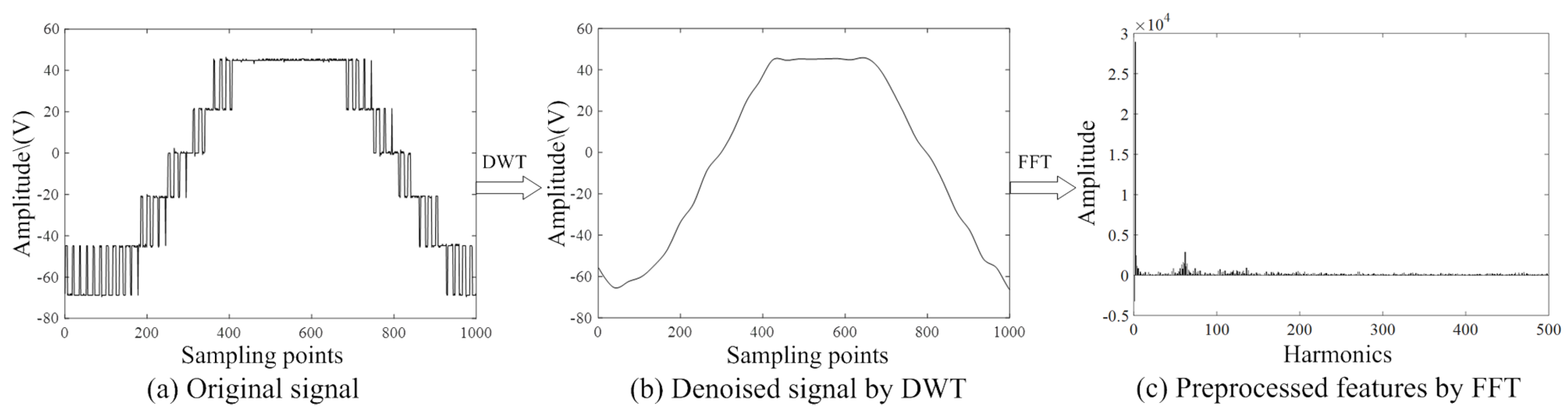
Additionally, if OC fault occurs at HS, the original signal, denoised signal by DWT and its spectrum by FFT-based preprocessing are shown in Figure 10. Compared with the original signal, the DWT-based denoised signal is smoother. It filters out some interference signals, such as the voltage pulses during the switching periods driven by SPWM. Therefore, it is also necessary to denoise original signals to enhance performance of fault diagnosis.
6. Conclusions
In order to solve the main problem that the fault signals at the cross positions of the last H-bridge in CHMI are very similar with each other, and affected by noise, leading to poor performance of fault diagnosis, the PCR method for better feature representation has been proposed in this paper. The proposed method includes the PCA-based feature extraction, features rearrangement of each PC and new projection matrix rebuilding. To reduce the noise interference, DWT by multiscale wavelet decomposition and reconstruction is used for signal denoising. To exact and select more useful features, FFT is used for signal preprocessing before the feature representation based on PCR. Furthermore, BPNN is used as a fault classification method to test the effectiveness and accuracy of the strategy based on PCR. It should be noted that other fault classification methods can also be used.
Moreover, a hardware platform based on a 7-level CHMI is built for assessing the performance of FFT-PCR-BPNN. The original experimental data are processed by different fault diagnosis strategies. By comparing and analyzing the results, the diagnosis strategy based on the proposed PCR requires less running time and achieves higher accuracy of fault diagnosis of CHMI. The concept that the features can be rearranged for better classification can be used for other feature representation methods, not only for PCA. By using the features from PCR, this paper provides an effective way to solve fault diagnosis in the presence of similar features and noise.
Acknowledgments
This work is supported by the National Natural Science Foundation of China (Grant No. 61673260), and the Natural Science Foundation of Shanghai (Grant No. 16ZR1414300).
Author Contributions
Zhuo Liu built the experimental platform, implemented experiments, collected the data and wrote the paper; Tianzhen Wang and Tianhao Tang analyzed the data and gave the directions; Yide Wang gave the modifications and suggestions of the proposed method, promoting the completion of the manuscript.
Conflicts of Interest
The authors declare no conflict of interest.
Abbreviations
The following abbreviations are used in this manuscript:
| CHMI | Cascaded H-bridge Multilevel Inverter |
| HS | H-bridge m, Switch |
| PCA | Principal Component Analysis |
| PCR | Principal Components Rearrangement |
| PCs | Principal Components |
| OC | Open Circuit |
| SC | Short Circuit |
References
- Choi, U.M.; Jeong, H.G.; Lee, K.B.; Blaabjerg, F. Method for Detecting an Open-Switch Fault in a Grid-Connected NPC Inverter System. IEEE Trans. Power Electron. 2012, 27, 2726–2739. [Google Scholar] [CrossRef]
- Babaei, E.; Alilu, S.; Laali, S. A New General Topology for Cascaded Multilevel Inverters with Reduced Number of Components Based on Developed H-Bridge. IEEE Trans. Ind. Electron. 2014, 61, 3932–3939. [Google Scholar] [CrossRef]
- Wang, L.; Zhang, D.; Wang, Y.; Wu, B.; Athab, H.S. Power and Voltage Balance Control of a Novel Three-Phase Solid-State Transformer Using Multilevel Cascaded H-Bridge Inverters for Microgrid Applications. IEEE Trans. Power Electron. 2016, 31, 3289–3301. [Google Scholar] [CrossRef]
- Chebabhi, A.; Fellah, M.K.; Kessal, A.; Benkhoris, M.F. A new balancing three level three dimensional space vector modulation strategy for three level neutral point clamped four leg inverter based shunt active power filter controlling by nonlinear back stepping controllers. ISA Trans. 2016, 63, 328–342. [Google Scholar] [CrossRef]
- Babaei, E.; Laali, S.; Bayat, Z. A single-phase cascaded multilevel inverter based on a new basic unit with reduced number of power switches. IEEE Trans. Ind. Electron. 2015, 62, 922–929. [Google Scholar] [CrossRef]
- Amini, J.; Moallem, M. A Fault-Diagnosis and Fault-Tolerant Control Scheme for Flying Capacitor Multilevel Inverters. IEEE Trans. Ind. Electron. 2017, 64, 1818–1826. [Google Scholar] [CrossRef]
- Choi, U.M.; Lee, J.S.; Blaabjerg, F.; Lee, K.B. Open-circuit fault diagnosis and fault-tolerant control for a grid-connected NPC inverter. IEEE Trans. Power Electron. 2016, 31, 7234–7247. [Google Scholar] [CrossRef]
- Potamianos, P.G.; Mitronikas, E.D.; Safacas, A.N. Open-circuit fault diagnosis for matrix converter drives and remedial operation using carrier-based modulation methods. IEEE Trans. Ind. Electron. 2014, 61, 531–545. [Google Scholar] [CrossRef]
- Wang, F.; Wang, Y.; Huang, X.X.; Zhang, Y.K. Fault Diagnosis of Inverter Power Supply Device Based on SVM. In Robotic Welding, Intelligence and Automation; Springer: New York, NY, USA, 2015; pp. 427–436. [Google Scholar]
- Jung, S.M.; Park, J.S.; Kim, H.W.; Cho, K.Y.; Youn, M.J. An MRAS-based diagnosis of open-circuit fault in PWM voltage-source inverters for PM synchronous motor drive systems. IEEE Trans. Power Electron. 2013, 28, 2514–2526. [Google Scholar] [CrossRef]
- Liu, Z.; Guo, W.; Hu, J.; Ma, W. A hybrid intelligent multi-fault detection method for rotating machinery based on RSGWPT, KPCA and Twin SVM. ISA Trans. 2017, 66, 249–261. [Google Scholar] [CrossRef] [PubMed]
- Zhang, J.; Zhu, Y.; Shi, W.; Sheng, G.; Chen, Y. An improved machine learning scheme for data-driven fault diagnosis of power grid equipment. In Proceedings of the 2015 IEEE 17th International Conference on High Performance Computing and Communications (HPCC), 2015 IEEE 7th International Symposium on Cyberspace Safety and Security (CSS), 2015 IEEE 12th International Conferen on Embedded Software and Systems (ICESS), New York, NY, USA, 24–26 August 2015; pp. 1737–1742. [Google Scholar]
- Cai, B.; Zhao, Y.; Liu, H.; Xie, M. A data-driven fault diagnosis methodology in three-phase inverters for PMSM drive systems. IEEE Trans. Power Electron. 2017, 32, 5590–5600. [Google Scholar] [CrossRef]
- Tang, Q.; Dai, J.; Liu, J.; Liu, C.; Liu, Y.; Ren, C. Quantitative detection of defects based on Markov–PCA–BP algorithm using pulsed infrared thermography technology. Infrared Phys. Technol. 2016, 77, 144–148. [Google Scholar] [CrossRef]
- Hao, X.; Jian, Z.; Jie, Q.; Tianzhen, W.; Jingang, H. RPCA-SVM fault diagnosis strategy of cascaded H-bridge multilevel inverters. In Proceedings of the 2014 International Conference on Green Energy, Sfas, Tunisia, 25–27 March 2014; pp. 164–169. [Google Scholar]
- Ni, J.; Zhang, C.; Yang, S.X. An adaptive approach based on KPCA and SVM for real-time fault diagnosis of HVCBs. IEEE Trans. Power Deliv. 2011, 26, 1960–1971. [Google Scholar] [CrossRef]
- Wang, T.Z.; Tang, T.H.; Wen, C.L.; Huang, H.Q. Relative principal component analysis algorithm and its application in fault detection. J. Syst. Simul. 2007, 13, 004. [Google Scholar]
- Geiger, B.C.; Kubin, G. Relative information loss in the PCA. In Proceedings of the 2012 IEEE Information Theory Workshop (ITW), Lausanne, Switzerland, 3–7 September 2012; pp. 562–566. [Google Scholar]
- Lv, Z.; Yan, X.; Jiang, Q. Batch process monitoring based on multiple-phase online sorting principal component analysis. ISA Trans. 2016, 64, 342–352. [Google Scholar] [CrossRef] [PubMed]
- Zhou, F.; Park, J.H.; Liu, Y. Differential feature based hierarchical PCA fault detection method for dynamic fault. Neurocomputing 2016, 202, 27–35. [Google Scholar] [CrossRef]
- Zhou, N.; Cheng, H.; Pedrycz, W.; Zhang, Y.; Liu, H. Discriminative sparse subspace learning and its application to unsupervised feature selection. ISA Trans. 2016, 61, 104–118. [Google Scholar] [CrossRef] [PubMed]
- Wang, T.; Qi, J.; Xu, H.; Wang, Y.; Liu, L.; Gao, D. Fault diagnosis method based on FFT-RPCA-SVM for cascaded-multilevel inverter. ISA Trans. 2016, 60, 156–163. [Google Scholar] [CrossRef] [PubMed]
- Shu, C.; Ya-Ting, C.; Tian-Jian, Y.; Xun, W. A novel diagnostic technique for open-circuited faults of inverters based on output line-to-line voltage model. IEEE Trans. Ind. Electron. 2016, 63, 4412–4421. [Google Scholar] [CrossRef]
- Hao, X.; Tianzhen, W.; Tianhao, T.; Benbouzid, M. A PCA-mRVM fault diagnosis strategy and its Application in CHMLIS. In Proceedings of the IECON 2014—40th Annual Conference of the IEEEIndustrial Electronics Society, Dallas, TX, USA, 29 October–1 November 2014; pp. 1124–1130. [Google Scholar]
- Zhang, S.; Tang, Q.; Lin, Y.; Tang, Y. Fault detection of feed water treatment process using PCA-WD with parameter optimization. ISA Trans. 2017, 68, 313–326. [Google Scholar] [CrossRef] [PubMed]
- Vijayakumari, B.; Devi, J.G.; Mathi, M.I. Analysis of noise removal in ECG signal using symlet wavelet. In Proceedings of the 2016 International Conference on Computing Technologies and Intelligent Data Engineering (ICCTIDE2016), Tamilnadu, India, 7–9 January 2016; pp. 1–6. [Google Scholar]
- Ellmauthaler, A.; Pagliari, C.L.; da Silva, E.A. Multiscale image fusion using the undecimated wavelet transform with spectral factorization and nonorthogonal filter banks. IEEE Trans. Image Process. 2013, 22, 1005–1017. [Google Scholar] [CrossRef] [PubMed]
- Shete, S.; Shriram, R. Comparison of Sub-band Decomposition and Reconstruction of EEG Signal by Daubechies9 and Symlet9 Wavelet. In Proceedings of the 2014 Fourth International Conference on Communication Systems and Network Technologies (CSNT), Gwalior, India, 7–9 April 2014; pp. 856–861. [Google Scholar]
- Meher, P.K.; Mohanty, B.K.; Patel, S.K.; Ganguly, S.; Srikanthan, T. Efficient VLSI architecture for decimation-in-time fast Fourier transform of real-valued data. IEEE Trans. Circuits Syst. I Regul. Pap. 2015, 62, 2836–2845. [Google Scholar] [CrossRef]
- Chang, H.H.; Linh, N.V. Statistical Feature Extraction for Fault Locations in Nonintrusive Fault Detection of Low Voltage Distribution Systems. Energies 2017, 10, 611. [Google Scholar] [CrossRef]
- Liu, S.; Hou, Z.; Yin, C. Data-driven modeling for UGI gasification processes via an enhanced genetic BP neural network with link switches. IEEE Trans. Neural Netw. Learn. Syst. 2016, 27, 2718–2729. [Google Scholar] [CrossRef]
- Yin, Z.; Hou, J. Recent advances on SVM based fault diagnosis and process monitoring in complicated industrial processes. Neurocomputing 2016, 174, 643–650. [Google Scholar] [CrossRef]
- Lei, Y.; Liu, Z.; Wu, X.; Li, N.; Chen, W.; Lin, J. Health condition identification of multi-stage planetary gearboxes using a mRVM-based method. Mech. Syst. Signal Process. 2015, 60, 289–300. [Google Scholar] [CrossRef]
- Peng, T.; Zhou, J.; Zhang, C.; Fu, W. Streamflow Forecasting Using Empirical Wavelet Transform and Artificial Neural Networks. Water 2017, 9, 406. [Google Scholar] [CrossRef]
- Tsai, J.T.; Chang, C.C.; Chen, W.P.; Chou, J.H. Data-Driven Modeling Using System Integration Scaling Factors and Positioning Performance of an Exposure Machine System. IEEE Access 2017, 5, 7826–7838. [Google Scholar] [CrossRef]
- Vargas, R.; Figueroa, A.; DeLeon, S.; Aguayo, J.; Hernandez, L.; Rodriguez, M. Analysis of Minimum Modulation for the 9-Level Multilevel Inverter in Asymmetric Structure. IEEE Lat. Am. Trans. 2015, 13, 2851–2858. [Google Scholar] [CrossRef]
- Wang, T.; Xu, H.; Han, J.; Elbouchikhi, E.; Benbouzid, M.E.H. Cascaded H-bridge multilevel inverter system fault diagnosis using a PCA and multiclass relevance vector machine approach. IEEE Trans. Power Electron. 2015, 30, 7006–7018. [Google Scholar] [CrossRef]
- Yan, Y.; Li, J.; Gao, D.W. Condition parameter modeling for anomaly detection in wind turbines. Energies 2014, 7, 3104–3120. [Google Scholar] [CrossRef]
Figure 1.
A Cascaded H-bridge Multilevel Inverter (CHMI) topology.
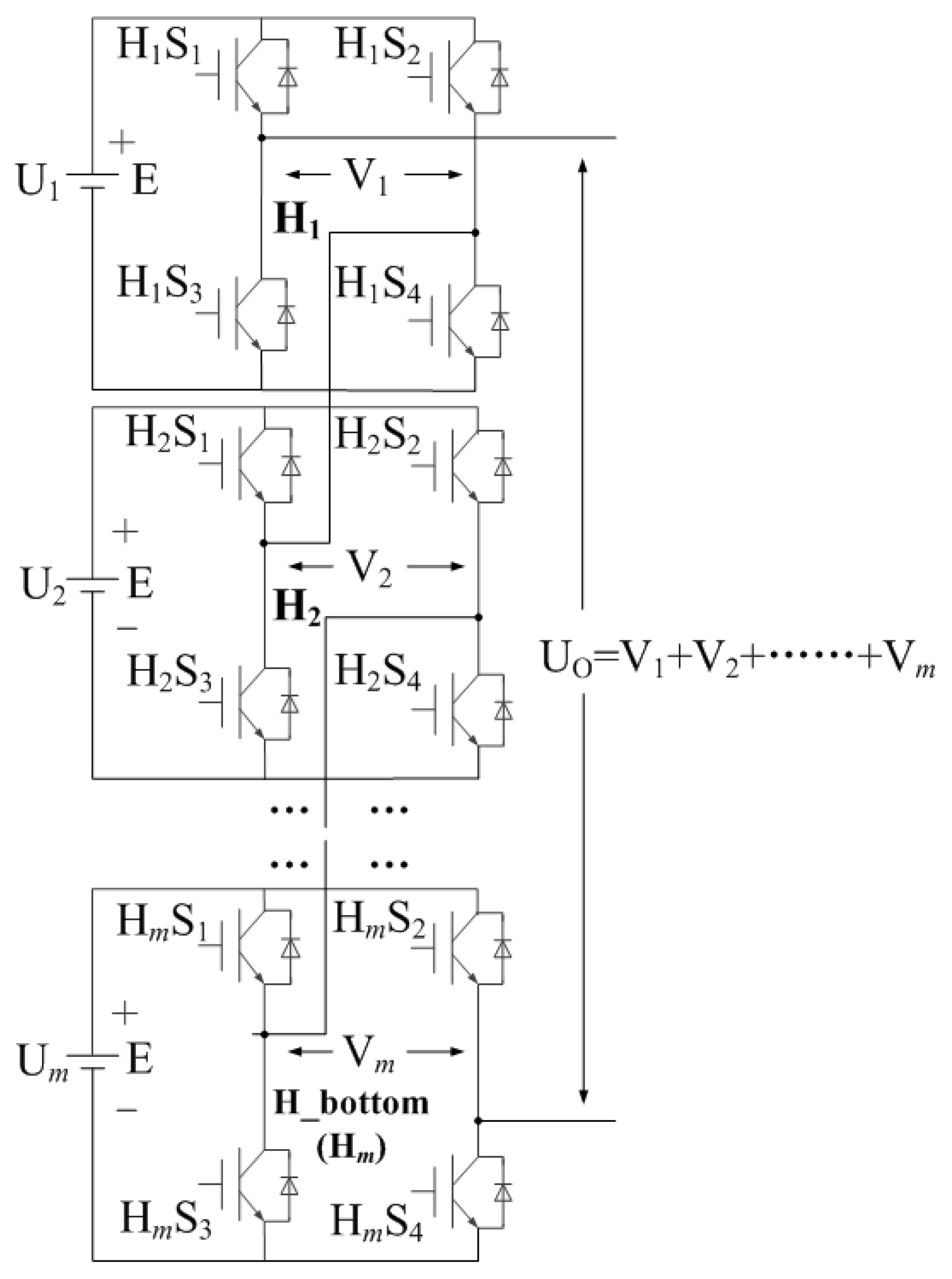
Figure 2.
Voltage signals of each switching device in a 7-level CHMI with load of infinite value when an Open Circuit (OC) occurs at 0.02 s.
Figure 2.
Voltage signals of each switching device in a 7-level CHMI with load of infinite value when an Open Circuit (OC) occurs at 0.02 s.

Figure 3.
Structure of the original data.
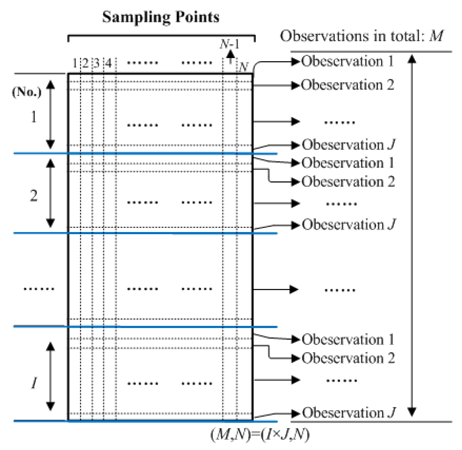
Figure 4.
Fault signals of CHMI with load = 5 when an Open Circuit (OC) occurs at 0 s and m = 3.

Figure 5.
Fault signals in H_bottom of CHMI when m = 4, 5, 6 and load = 5 .
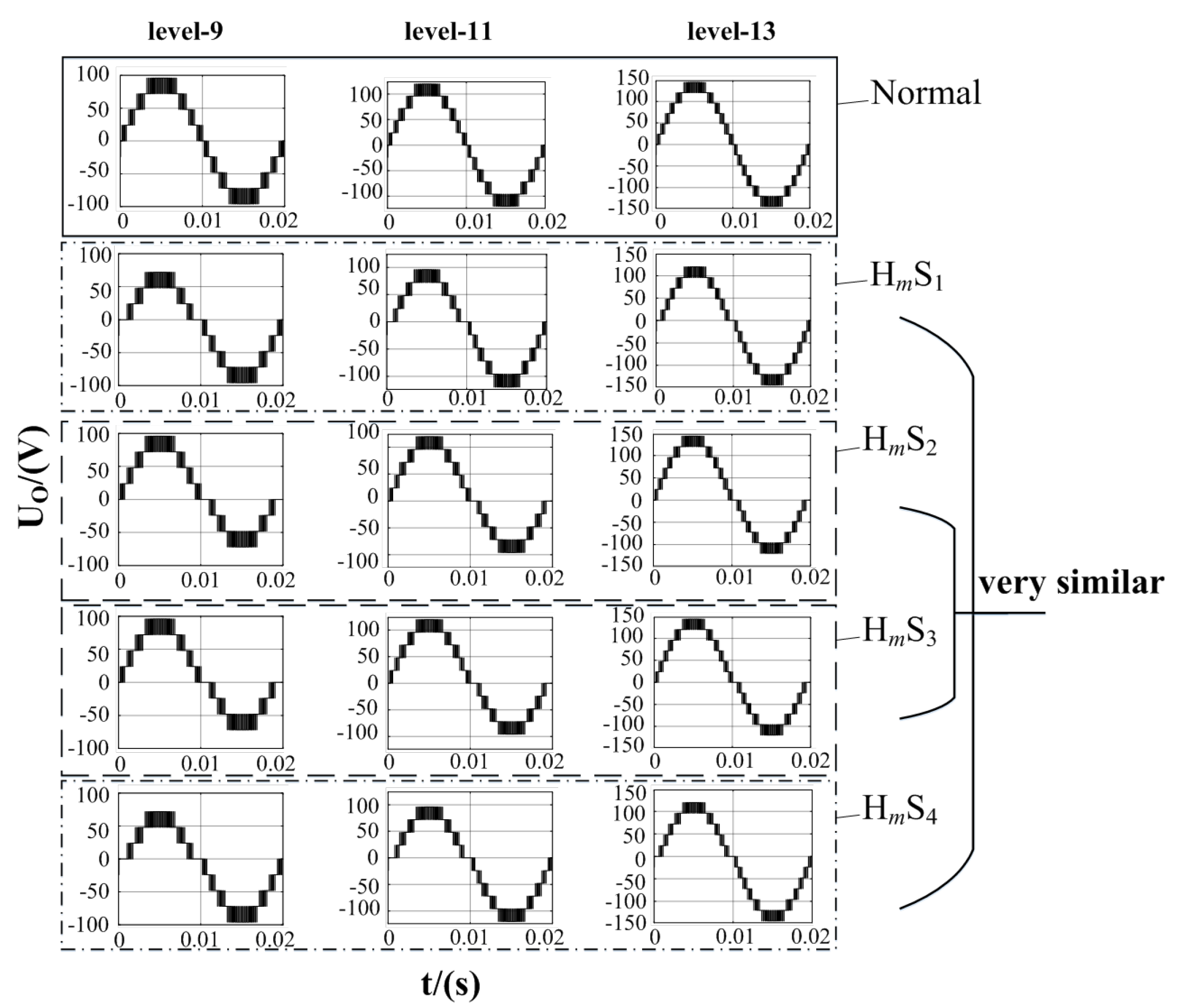
Figure 6.
Structure of fault diagnosis strategy used in the inverter system.
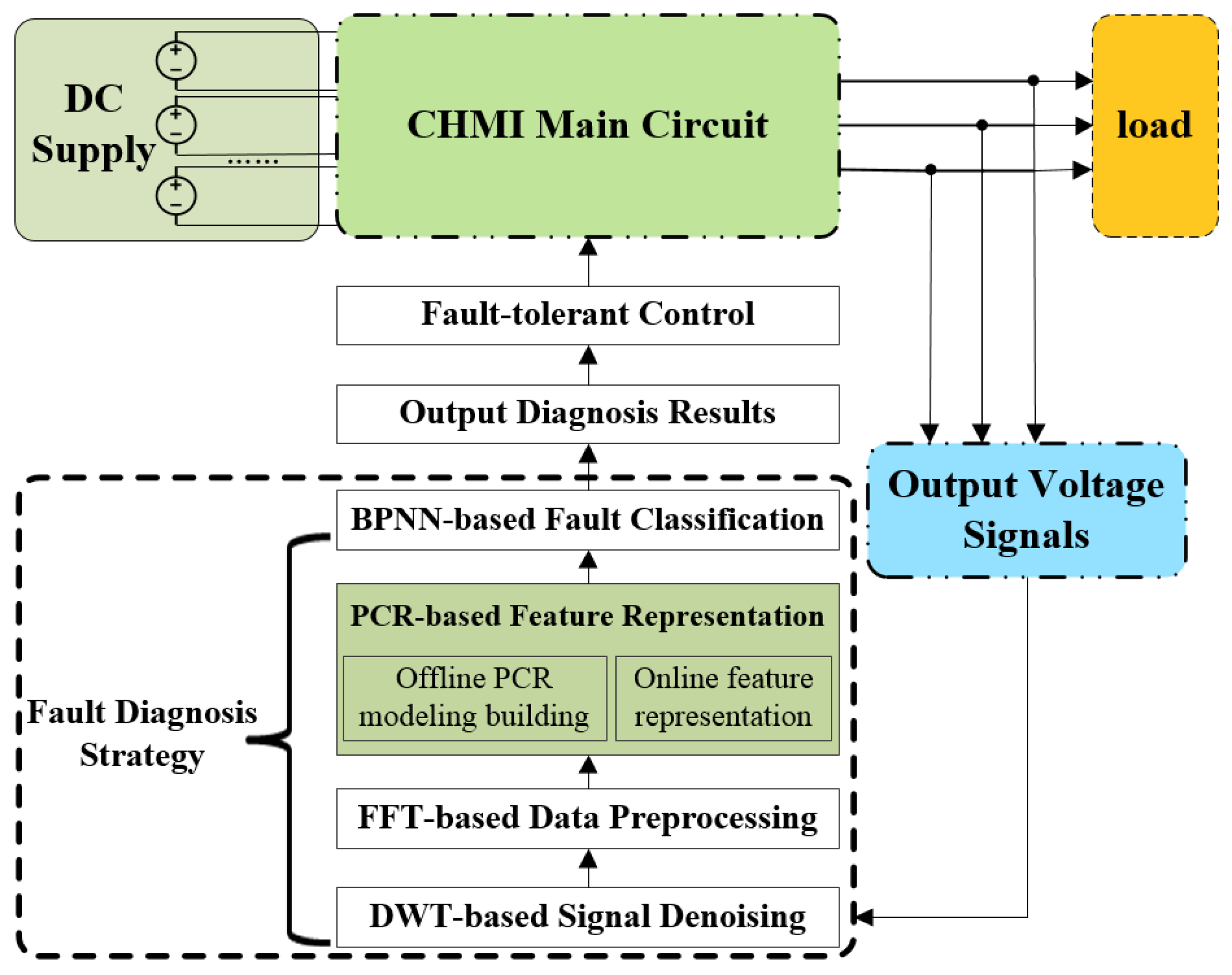
Figure 7.
Framework of the using process based on Principal Components Rearrangement (PCR).
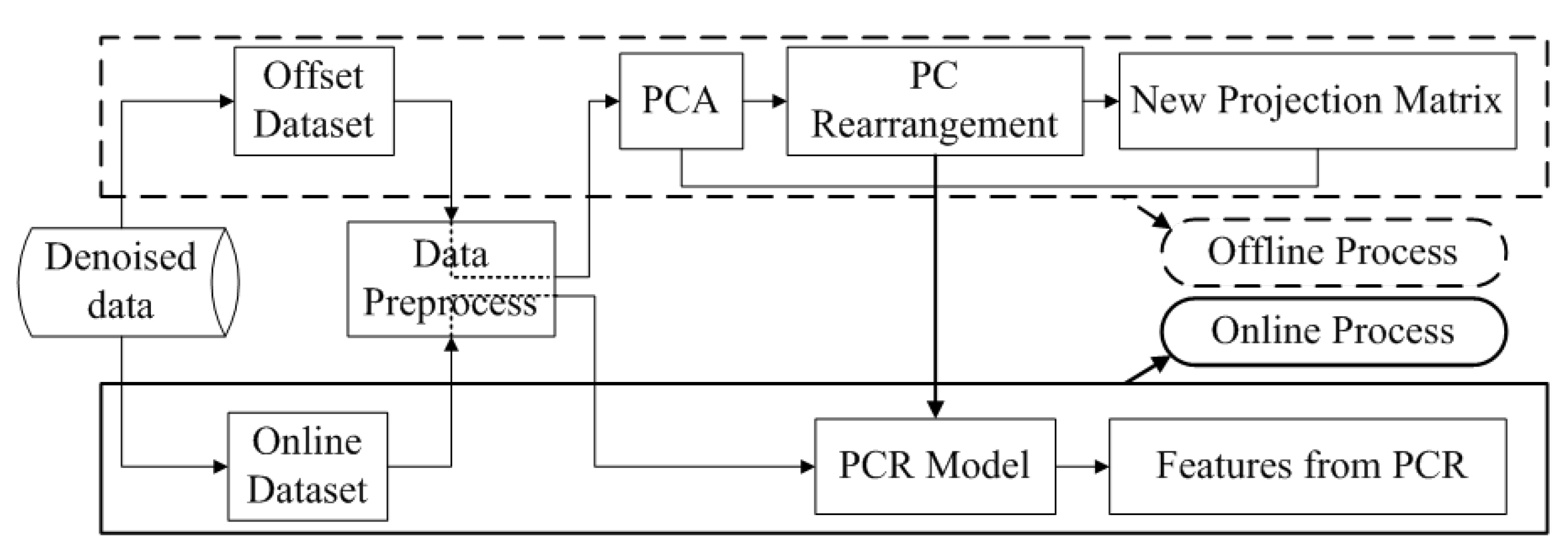
Figure 8.
Hardware platform of cascaded H-bridge inverter.
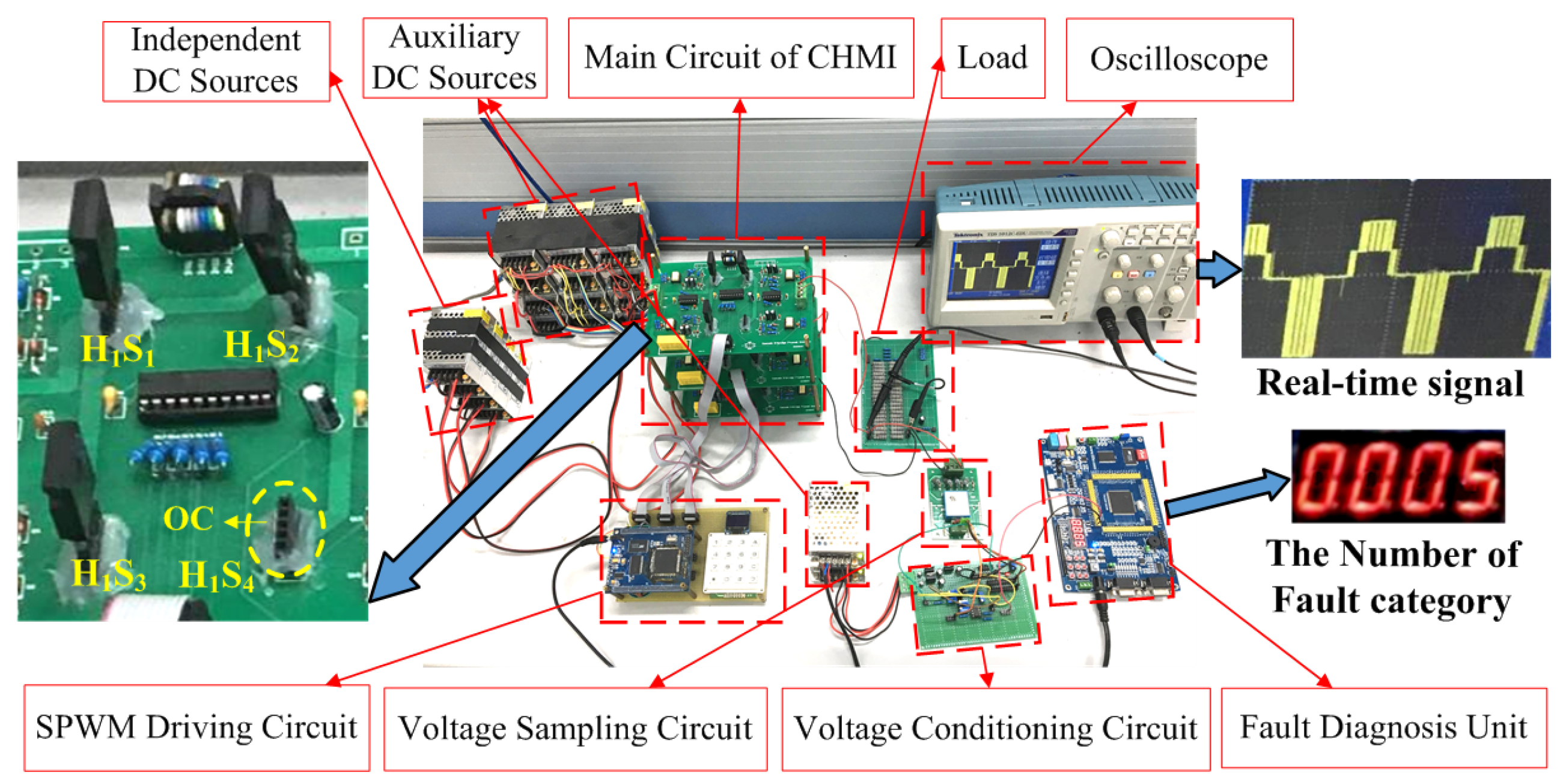
Figure 9.
Data spectra.

Figure 10.
Processed results of original signal after denoising and preprocessing when HS has an Open Circuit (OC) fault.
Figure 10.
Processed results of original signal after denoising and preprocessing when HS has an Open Circuit (OC) fault.


Table 1.
Faults and category labels.
| No. | Fault | Category Labels |
|---|---|---|
| 1 | Normal | [1,0,0,0,0,0,0,0,0,…,0,0,0,0] |
| 2 | H-bridge 1, Switch 1 Open Circuit (HS OC) | [0,1,0,0,0,0,0,0,0,…,0,0,0,0] |
| 3 | HS OC | [0,0,1,0,0,0,0,0,0,…,0,0,0,0] |
| 4 | HS OC | [0,0,0,1,0,0,0,0,0,…,0,0,0,0] |
| 5 | HS OC | [0,0,0,0,1,0,0,0,0,…,0,0,0,0] |
| 6 | HS OC | [0,0,0,0,0,1,0,0,0,…,0,0,0,0] |
| 7 | HS OC | [0,0,0,0,0,0,1,0,0,…,0,0,0,0] |
| 8 | HS OC | [0,0,0,0,0,0,0,1,0,…,0,0,0,0] |
| 9 | HS OC | [0,0,0,0,0,0,0,0,1,…,0,0,0,0] |
| ⋯ | ⋯ | ⋯ |
| 4m−2 | HS OC | [0,0,0,0,0,0,0,0,0,…,1,0,0,0] |
| 4m−1 | HS OC | [0,0,0,0,0,0,0,0,0,…,0,1,0,0] |
| 4m | HS OC | [0,0,0,0,0,0,0,0,0,…,0,0,1,0] |
| 4m+1 | HS OC | [0,0,0,0,0,0,0,0,0,…,0,0,0,1] |
Table 2.
Main parameters of the system.
| Notation | Description | Value/Product Model |
|---|---|---|
| Voltage of DC sources | 24 V | |
| Load | Impedance of the load in Cascaded H-bridge Multilevel Inverter (CHMI) | |
| Voltage sampling unit | CHV-25P/200 | |
| Insulated Gate Bipolar Transistor (IGBT) | Switching device | AUIRGP35B60PD |
| Optocoupler | Drive isolation modules | TLP250 |
| Digital Signal Processor (DSP) | Controlling chip | TMSF28335 |
| Oscilloscope | For monitoring and data acquisition | TDS 1012C-EDU |
| 7-level CHMI | Main circuit of CHMI | With 3 H-bridges |
Table 3.
Main parameters of the fault diagnosis strategy.
| Notation | Description | Value/Product Model |
|---|---|---|
| M | Number of all the observations | 5200 |
| N | Sampling points in each observation | 1000 |
| I | Number of fault categories | 13 |
| J | Observations in each category | 400 |
| Wavelet function | sym8 | |
| Decomposition layers by Discrete Wavelet Transform (DWT) | 5 | |
| Modulation ratio of Sinusoidal Pulse Width Modulation (SPWM) | 0.85–0.95 | |
| SPWM | Method of driving switching devices | Phase Disposition SPWM [36] |
| Switching frequency | 1 kHz | |
| Experimental sample frequency | 50 kHz | |
| Cumulative Percentage of Variance (CPV) | CPV value in principal component analysis method | 0.95 |
| Pseudoinverse matrix of X | Singular Value Decomposition (SVD) | |
| The limit of minimum value of S in SVD | ||
| The output layer nodes of Back Propagation Neural Network (BPNN) | 13 | |
| Activation function |
Table 4.
Average fault diagnostic results based on different diagnosis strategies and the parameters of Back Propagation Neural Network (BPNN).
Table 4.
Average fault diagnostic results based on different diagnosis strategies and the parameters of Back Propagation Neural Network (BPNN).
| Items | Fault Diagnosis Strategies and Parameters of BPNN | Test Samples (Groups) | ||||
|---|---|---|---|---|---|---|
| 3 | 50 | 71 | 92 | |||
| Running time (ms) | FFT-BPNN | = 70, = 19, learning rate = 0.50 | 1725 | 1861 | 1710 | 1693 |
| PCA-BPNN | = 8, = 14, learning rate = 0.20 | 923 | 917 | 946 | 904 | |
| FFT-PCA-BPNN | = 2, = 13, learning rate = 0.18 | 561 | 529 | 532 | 595 | |
| PCR-BPNN | = 8, = 14, learning rate = 0.20 | 101 | 129 | 113 | 128 | |
| FFT-PCR-BPNN | = 2, = 13, learning rate = 0.18 | 34.7 | 36.9 | 41.2 | 30.8 | |
| Diagnostic accuracy (%) | FFT-BPNN | Same as above | 82.8 | 81.5 | 81.9 | 80.7 |
| PCA-BPNN | 84.8 | 83.6 | 84.5 | 83.3 | ||
| FFT-PCA-BPNN | 92.9 | 93.5 | 93.1 | 93.2 | ||
| PCR-BPNN | 95.2 | 94.9 | 94.6 | 95.7 | ||
| FFT-PCR-BPNN | 99.5 | 99.7 | 99.3 | 99.6 | ||
© 2017 by the authors. Licensee MDPI, Basel, Switzerland. This article is an open access article distributed under the terms and conditions of the Creative Commons Attribution (CC BY) license (http://creativecommons.org/licenses/by/4.0/).
Share and Cite
MDPI and ACS Style
Liu, Z.; Wang, T.; Tang, T.; Wang, Y. A Principal Components Rearrangement Method for Feature Representation and Its Application to the Fault Diagnosis of CHMI. Energies 2017, 10, 1273. https://doi.org/10.3390/en10091273
AMA Style
Liu Z, Wang T, Tang T, Wang Y. A Principal Components Rearrangement Method for Feature Representation and Its Application to the Fault Diagnosis of CHMI. Energies. 2017; 10(9):1273. https://doi.org/10.3390/en10091273
Chicago/Turabian StyleLiu, Zhuo, Tianzhen Wang, Tianhao Tang, and Yide Wang. 2017. "A Principal Components Rearrangement Method for Feature Representation and Its Application to the Fault Diagnosis of CHMI" Energies 10, no. 9: 1273. https://doi.org/10.3390/en10091273
Note that from the first issue of 2016, this journal uses article numbers instead of page numbers. See further details here.