Impacts of Power Grid Frequency Deviation on Time Error of Synchronous Electric Clock and Worldwide Power System Practices on Time Error Correction

Abstract

Synchronous electric clocks utilize power grid frequency as their timing reference. Power grid frequency deviation away from its nominal value results in synchronous electric clocks running fast or running slow (also known as the time error). In this article, statistical analysis on time error of synchronous electric clocks around the world is firstly presented using the power grid frequency measurements recorded by the wide-area frequency monitoring network FNET/GridEye. Then, the time error correction (TEC) process provided by electric utilities is analyzed and the worldwide TEC practice is investigated. Eventually, regions of the world where electric utilities provide TEC service are differentiated from those without TEC services. Analytical results demonstrate that the average time error of synchronous electric clocks in North America seems to be less than five seconds, and it has not changed very much over the past few years. On the other hand, the identification results present that up to the end of 2016, many electric utilities around the world, especially in North America and Europe, provided the TEC service to periodically remove the accumulative time error of synchronous electric clocks.

1. Introduction

A synchronous electric clock is powered by electricity and synchronous to the power line frequency. It was first constructed around the 1910s and became one of the most widely used clocks after the rapid development of electric power industry in the 1930s [1]. A synchronous electric clock does not contain a timekeeping oscillator such as a balance wheel, but instead it keeps the time through counting the oscillations of the electric current waveform from its wall plug [2]. An important reason for the popularity of synchronous electric clocks around the world is that the power grid frequency, as a clock timing source with almost zero cost, reliable performance and high accuracy, is generally accessible anywhere and anytime, as long as there are power transmission lines in service [3]. Nowadays, there are still many synchronous electric clocks using power grid frequency as their timing sources [4], for example, traffic lights, electricity meters and programmable household appliances. Therefore, the timekeeping ability of synchronous electric clock is important for people’s daily life.

However, power grid frequency is not always a constant (also known as the nominal frequency, it is 60 Hz in North and South America, but 50 Hz in most other countries). Electric utilities usually keep the power grid frequency running in a very small range. The frequency deviation away from its nominal value results in synchronous electric clocks running fast or running slow. If a power grid frequency is above its nominal value, the clock will run fast. Otherwise, it will run slow. Therefore, the fluctuation of power grid frequency might cause a time error of a few seconds during the period of one day [5]. This time error would not completely cancel out by its own. As time goes by, this error gradually accumulates and finally tends to cause a large time drift of synchronous electric clocks in the long term.

As discussed above, the stability of a power grid frequency has great influence on the timekeeping ability of synchronous electric clock. In fact, the frequency stability is considered as a critical issue for secure power system operation [6]. Therefore, a large number of studies on power system frequency stability have been performed over the last ten years, for example, frequency stability evaluation and control [7], the determination of frequency stability border of power system operation [8], the enhancement strategies to improve power system frequency stability [9,10], and the impact of renewable energy generation on frequency stability [11,12,13]. Although the frequency stability has been studied for many years, these studies mentioned above are primarily concerned with the ability of power system to maintain the steady frequency after a severe disturbance [14]. Up to now, there is a good deal of research focusing on the impacts of power system frequency deviation on the time error of synchronous electric clock.

In this paper, we used frequency measurements collected by the wide-area frequency monitoring network, FNET/GridEye, to carry out the detailed statistical analysis on the time error of synchronous electric clocks in both North American and worldwide power grids. As a pilot wide-area measurement system (WAMS) system, FNET/GridEye has been monitoring the U.S. power grids and other worldwide power grids for more than a decade. Using those valuable measurements, the time error correction (TEC) service provided by electric utilities was investigated through the data-driven approach. The TEC practice around the world was also analyzed. FNET/GridEye, as an independent observer, identified regions of the world where electric utilities are providing TEC services from those without TEC services. Considering that TEC services would end soon in North America [5], our research would be helpful to reveal the impacts of TEC services on the time error and provide valuable guidance for the future development of synchronous clocks. Finally, the long-term power system frequency distribution pattern was studied and its statistical characteristics were identified. To the best of our knowledge, it is the first effort to analyze the time error of synchronous electric clock in worldwide power grids and investigate the worldwide practice of the time error correction service provided by electric utilities.

The other sections of this paper are organized as follows. Section 2 presents a brief introduction of the wide-area frequency monitoring network FNET/GridEye. Statistical analysis on the time error of synchronous electric clock is shown in Section 3. Section 4 discusses two common types of TEC services and the worldwide TEC practice. Then, the long-term frequency distribution patterns in worldwide power grids are provided in Section 5. Finally, this paper is concluded in Section 6.

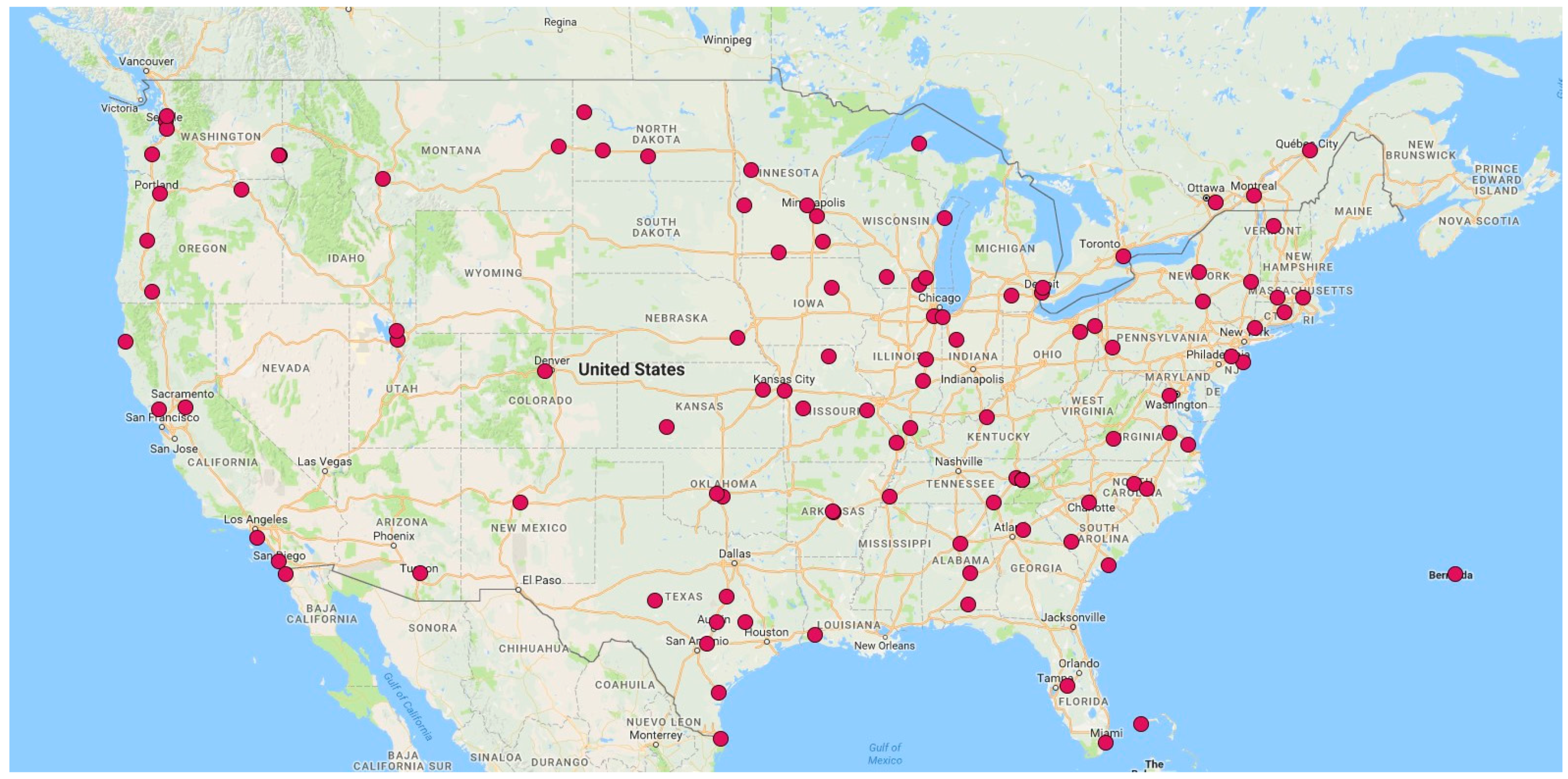
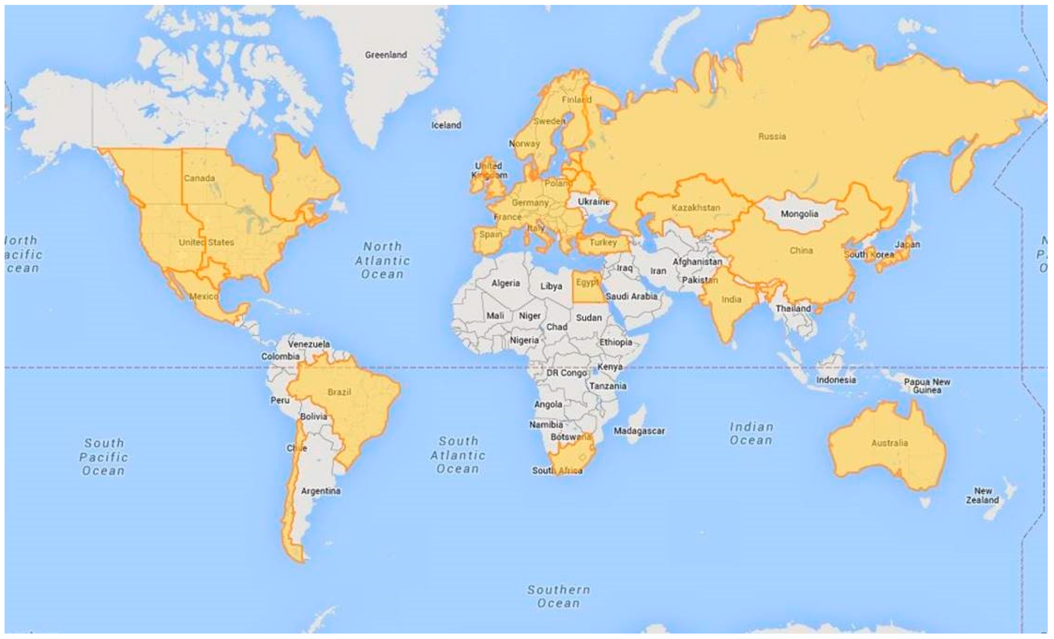
2. Wide-Area Frequency Monitoring Network FNET/GridEye

Obtaining the frequency measurement of power transmission line is a prerequisite for analyzing the timekeeping accuracy of synchronous electric clocks. The power grid frequency dataset used in this paper is provided by FNET/GridEye. As a pioneering WAMS, FNET/GridEye was originally developed in 2003 and is now operated by the University of Tennessee, Knoxville (UTK), and Oak Ridge National Laboratory (ORNL) [15].

FNET/GridEye, an internet-based WAMS, has been continuously monitoring the power grid for over ten years [16]. It can measure power grid frequency, voltage magnitude and voltage angle with low-cost, reliable performance and high accuracy (±0.0005 Hz for grid frequency and ±0.0002 rad for voltage angle) [17]. Since the FNET/GridEye went online in 2003, more than 15 TB of data have been collected. Based on these real-time measurements, a variety of online and offline applications have been developed to monitor power system dynamic behaviors, such as event location estimation [18], inter-area oscillation mode identification [19], and adaptive data-driven damping control [20].

The frequency disturbance recorder (FDR), a single-phase variant of the phasor measurement unit (PMU), is the main sensor of the FNET/GridEye [21]. In comparison with the conventional PMU, which requires high production and installation cost, the FDR measures from a normal single-phase electrical outlet at the 120 V distribution level [22]. These measurements are then synchronized by Global Positioning System (GPS)-based timestamps and transferred through Internet to the phasor data concentrator (PDC) for data processing and long-term storage [23]. After over ten years of development, more than 200 FDRs have been deployed in main interconnection systems of North America [24]. Figure 1 shows the location of FDRs deployed in North America up to now. On the other hand, the FNET/GridEye also serves other interconnection systems around the world. Up to now, over 50 FDRs have been deployed worldwide, for example, China, Europe and Japan [24]. Figure 2 demonstrates the FNET/GridEye sensor deployment around the world.

In this study, we select 12 FDRs deployed in different Interconnection systems around the world.

Table 1. Basic information of the selected FDRs in this study.

FDR	Location	Nominal Frequency
1	USA, Seattle	60 Hz
2	USA, Matton	60 Hz
3	Sweden, Stockholm	50 Hz
4	USA, San Angelo	60 Hz
5	Brazil, Itajubá	60 Hz
6	Japan, Karuizawa	60 Hz
7	UK, Sheffield	50 Hz
8	Denmark, Aalborg	50 Hz
9	China, Shanghai	50 Hz
10	Australia, Brisbane	50 Hz
11	India, Kanpur	50 Hz
12	Latvia, Riga	50 Hz

gives the basic information of all selected FDRs. For example, the first three FDRs record the frequency of Eastern Interconnection (EI), Western Electricity Coordinating Council (WECC) and Electric Reliability Council of Texas (ERCOT) systems in North America, respectively. The FDR deployed in Aalborg, Denmark collects the frequency of the synchronous grid of Continental Europe.

3. Statistical Analysis on Time Error of Synchronous Electric Clock

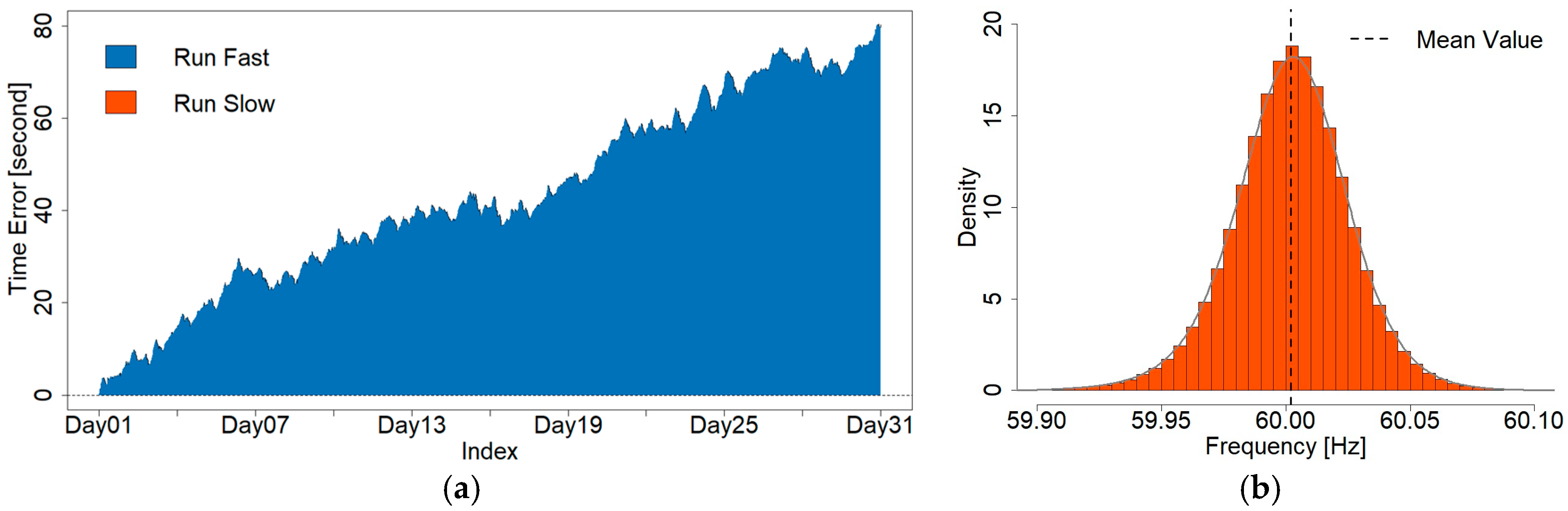
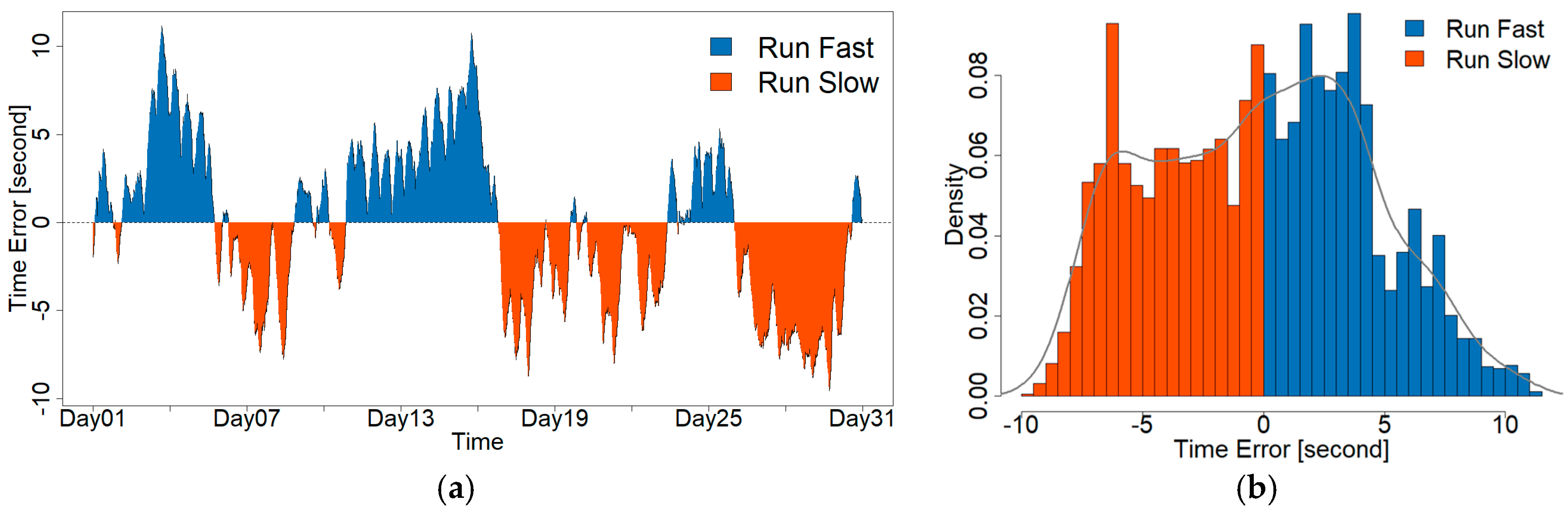
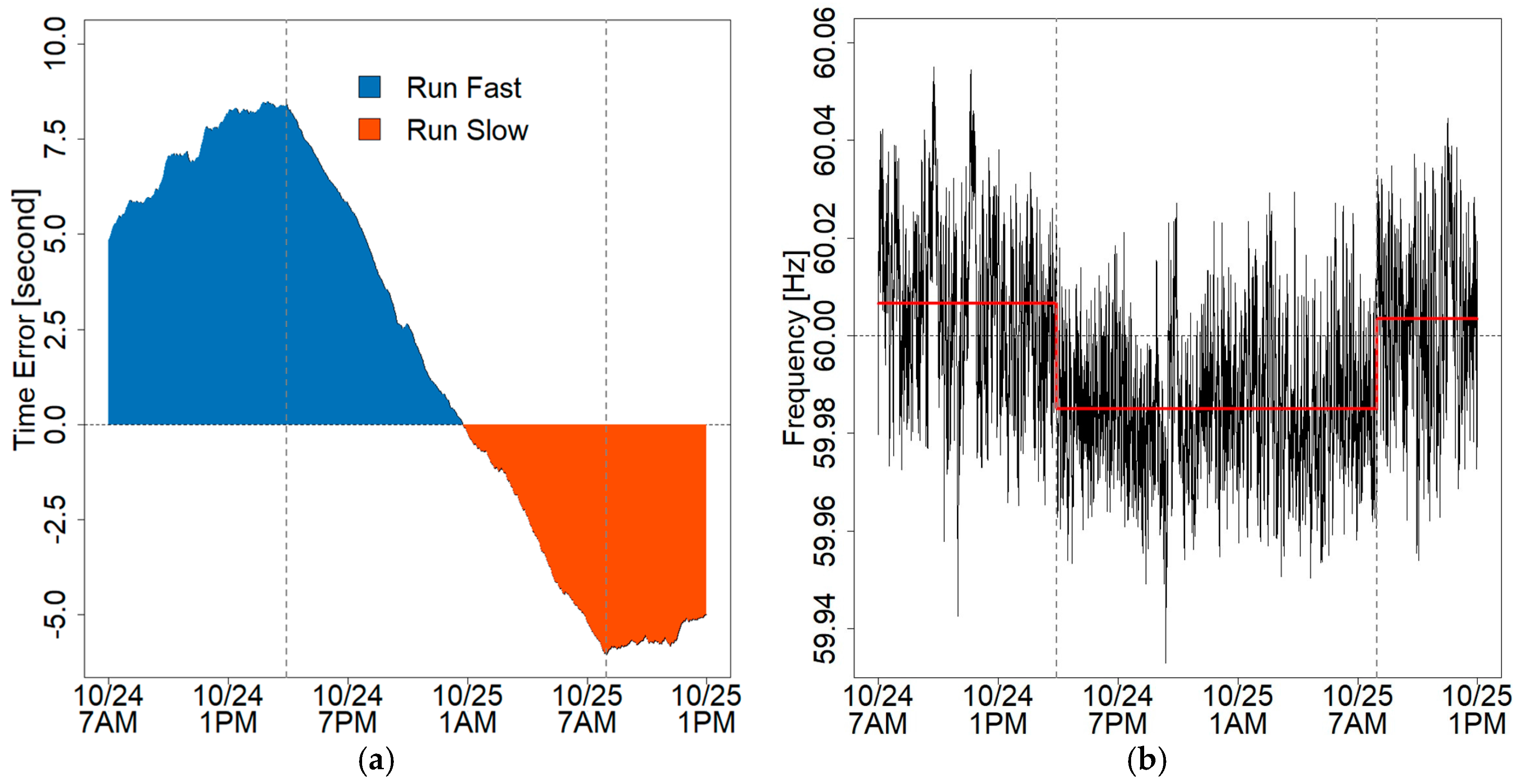
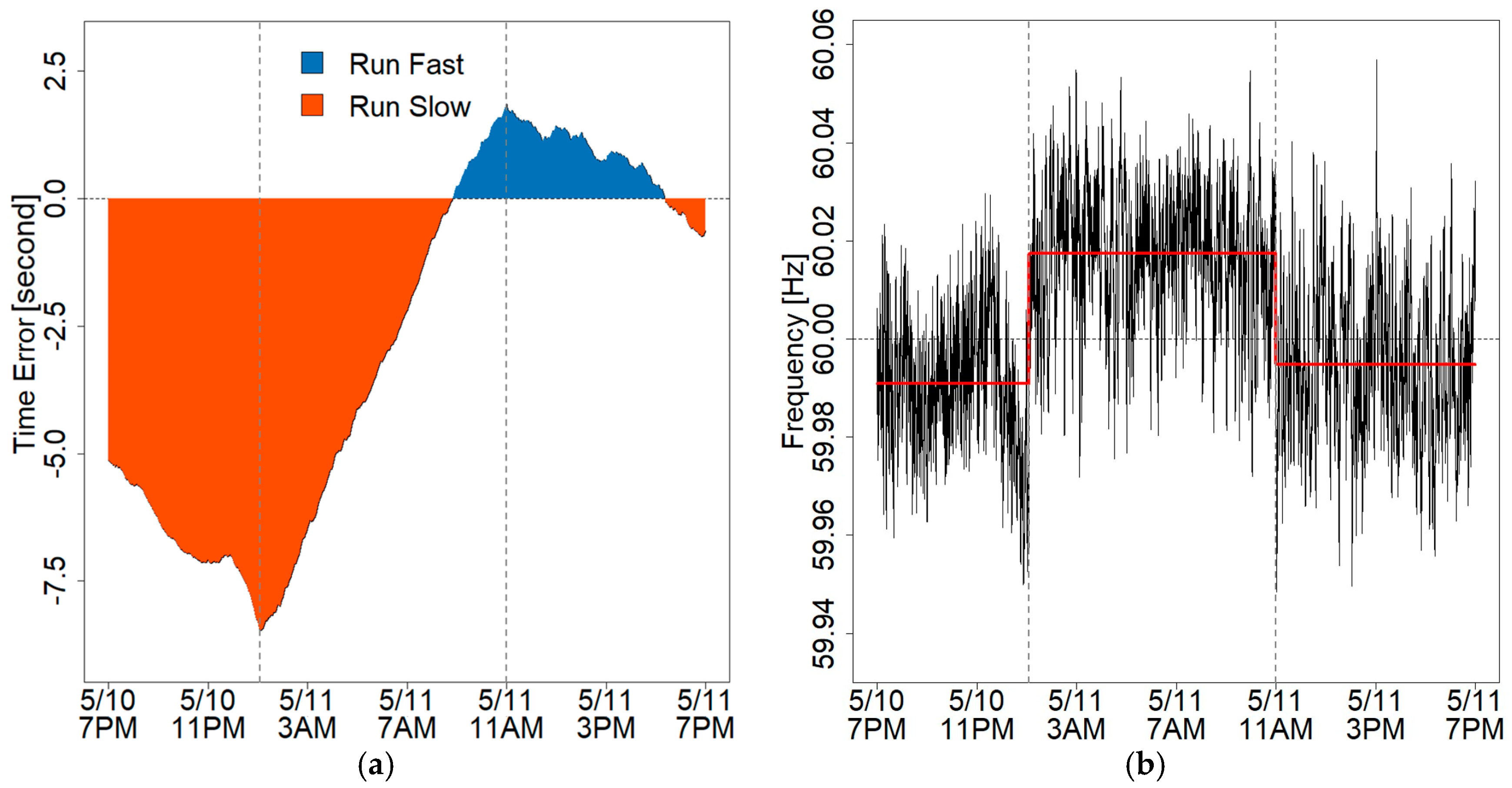
3.1. Time Error Calculation

In this study, we assume an ideal synchronous clock using power grid frequency, which means there is no time error inside this ideal clock. Then, we only consider the impact of the frequency deviation on its time error. The instantaneous time error at time t caused by frequency deviation can be written as:

$$\mathsf{∆}{T}_t=\frac{f_t-f^{*}}{f^{*}}\times \tau ,$$

(1)

where $f^{*}$ is the nominal frequency (60 Hz in North America), $f_t$ is the real-time frequency recorded by FNET/GridEye at time t. $\tau$ is the temporal resolution of frequency measurements. In this paper, $\tau$ = 0.1 because the FDR records power line frequency every 0.1 s. Then, the accumulative time error up to time t can be calculated by:

$$\mathsf{∆}T={\displaystyle \sum }_t\mathsf{∆}{T}_t,$$

(2)

According to Equations (1) and (2), if power line frequency has been running 2 mHz high (i.e., 60.002 Hz), a synchronous clock using this frequency as its timing reference would run fast 1.2 s after 10 h (i.e., 2 mHz/60 Hz × 10 h × 3600 s/h = 1.2 s).

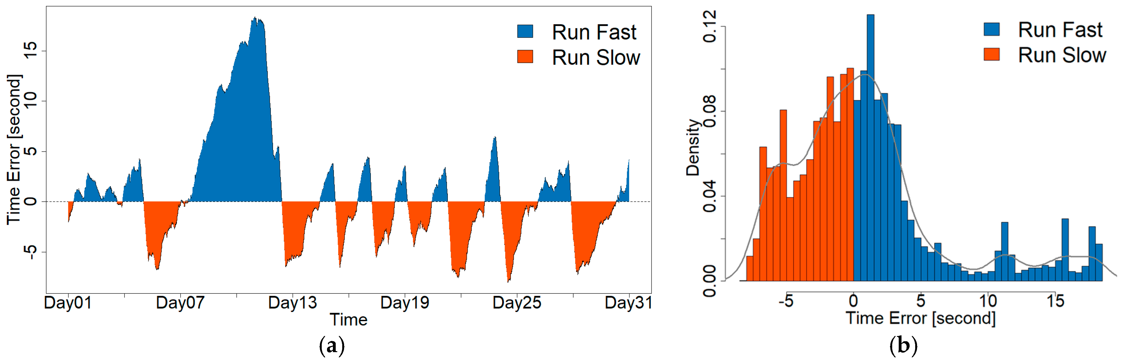
3.2. Time Error Analysis in North America

Figure 3 shows the change of the time error over one month in EI system of North America. This time error is displayed by an ideal synchronous clock. To compute the time error reasonably, the median time error over one month is set as the time reference of this ideal synchronous clock. If the time error gives a positive value, the clock runs fast. On the contrary, the negative time error indicates that the clock runs slow. From Figure 3a, it can be seen that the time error went up and down many times in one month. Although the maximum time error once reached up to about +18.38 s, the average time error was only +00.78 s, meaning the synchronous clock could likely run very well in EI system. Figure 3b presents the probabilistic distribution of time error in one month. From Figure 3b, it can be observed that the possibility of running fast seems to be quite close to the possibility of running slow.

Figure 4 presents the change of the time error in October 2016 for WECC system of North America. From Figure 4, it can be observed that the results of WECC system are similar to those of EI system shown in Figure 3. The accumulative time error changed from −09.58 to +11.14 s. From the time error distribution depicted in Figure 4b, it can be found that if the clock uses the WECC frequency as its timing reference, the possibility of running fast and running slow is quite close. The average time error was about +00.16 s.

Figure 5 shows the time error change in ERCOT system of North America with the same period of Figure 3 and Figure 4. Compared with EI and WECC systems, ERCOT system is a minor interconnection system because it only covers most, but not all, of Texas. From Figure 5a, it can be observed that the time error did not change sharply over one month. The maximum fast time error is +07.15 s and the maximum slow time error is −05.68 s. On the other hand, the time error distribution in Figure 5b demonstrates that the possibility of running fast is nearly equal to the possibility of running slow. The average time error over one month is +00.58 s, very close to zero.

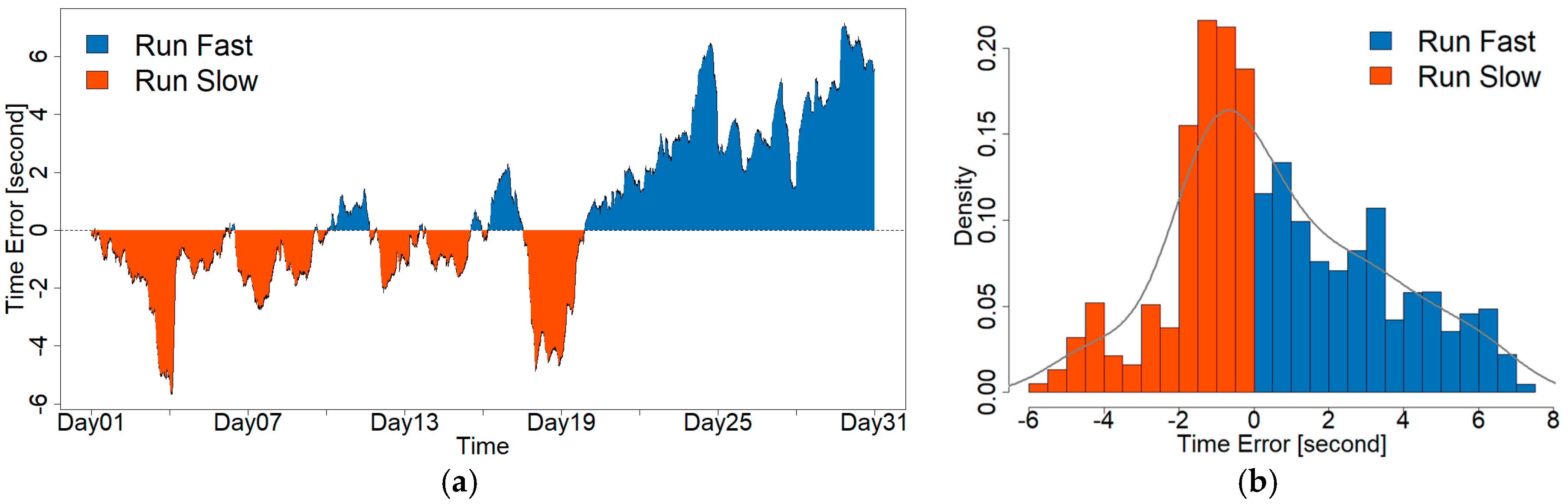
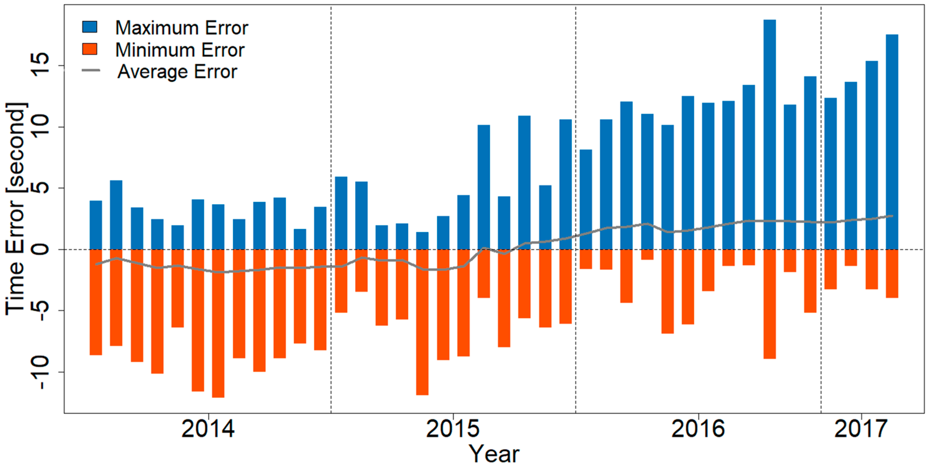
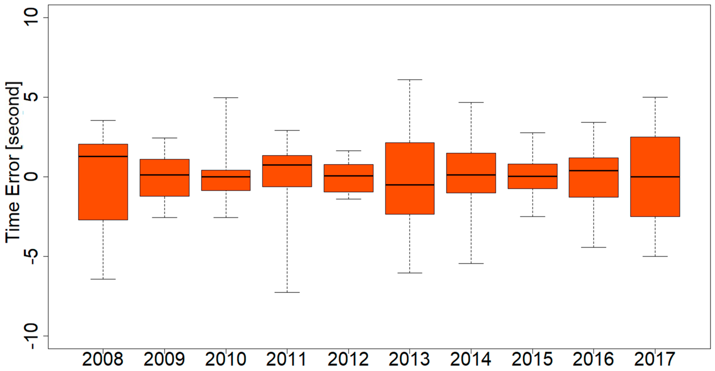
3.3. Time Error Tendency in Recent Years

Next, we analyze the changing tendency of time error over the past few years. In this subsection, three statistical indicators are calculated for each month and then their changes are used to study the time error trend. These three indicators include:

• Maximum Error (i.e., the maximum running fast time error over a specified period);
• Minimum Error (i.e., the maximum running slow time error over a specified period);
• Average Error (i.e., the average time error over a specified period).

Note that the maximum error always takes a positive value and the minimum error always takes a negative value. The average error can be either positive or negative. Figure 6 presents the monthly change of the above three indicators for EI system from January 2014 to April 2017. Note that the time error of each month has the same time reference. The time error of next month would cumulative upon the latest time error of previous month. From Figure 6, it can be seen that the maximum error seems to be gradually increasing over the past few years. In 2014, the monthly maximum error was generally less than +05.00 s. However, it has climbed up to above +10.00 s since 2016. By contrast, the monthly minimum error shows a downward trend in recent years. Its value decreased from nearly −10.00 s in 2014 to about −05.00 s in 2017. On the other hand, we also observe that the variation range of time error has a tendency to become large in recent years. Nevertheless, the average error did not change too much from 2014 to 2017 and its value was always lower than ±3.50 s, meaning that the clock can still work very well. Another interesting observation is that there was a turning point for the average error in September 2015. Before this turning point, the monthly average error was always negative. After this point, however, the average error turned to be a positive value, which means the synchronous clock was more likely to run faster than the standard time.

Texas produces the most wind power of any states in the USA. [25]. Wind power generation accounted for 12.63% of the total electricity generation in Texas during 2016. Figure 7 demonstrates the yearly change of the time error for ERCOT system from 2008 to 2017. In each year, a typical month is selected as a reference for calculating some statistics of the time error, including the maximum, minimum, median time error and their quartiles. In each month, the median time error over this month is set as the time reference. As shown in Figure 7, although the annual wind power generation has tripled from 2008 (16,225 GWh) to 2016 (57,551 GWh) in Texas [26], which may have negative impacts on power system frequency stability because of wind power fluctuation [27], there seems to be no obvious changes for these time error statistics. This might be because the ERCOT continues to provide TEC services to black out the accumulated time error when it arises. More information about TEC service is presented in Section 4. The accumulative time error was generally lower than ±10.00 s. Moreover, the average time error did not change too much over the past ten years and its value was always lower than ±02.00 s.

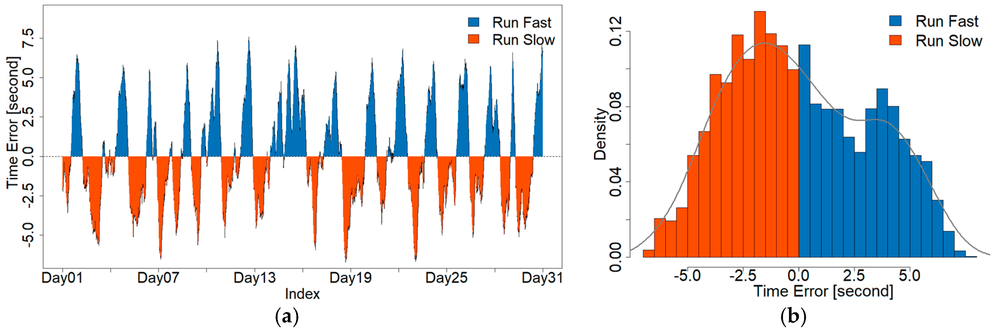
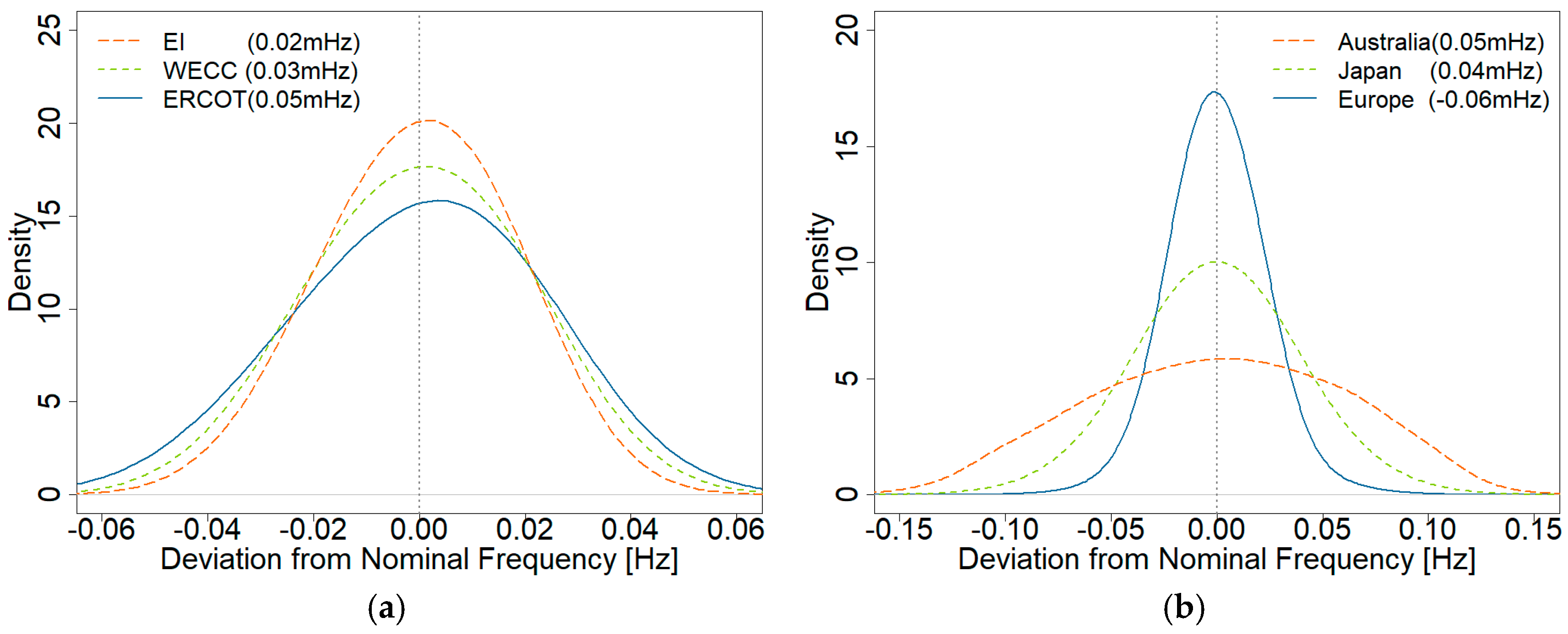
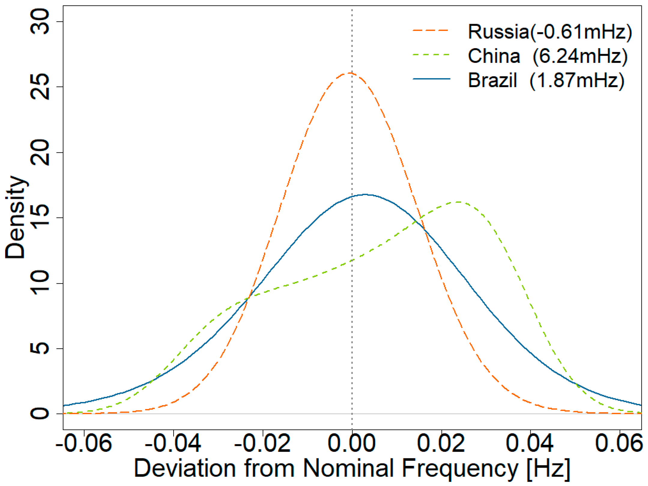
3.4. Time Error Analysis around the World

In addition to the three interconnection systems in North America discussed above, the time error of the synchronous clock using power grid frequency in worldwide power grids are also analyzed in this subsection.

Table 2. Statistical analysis of the monthly time error around the world.

Location	Maximum Time Error (Run Fast, Seconds)	Minimum Time Error (Run Slow, Seconds)	Average Time Error (Seconds)
USA, Seattle	+11.14	−09.58	+00.16
USA, Matton	+18.38	−08.05	+00.78
Sweden, Stockholm	+20.52	−12.11	+02.97
USA, San Angelo	+07.15	−05.68	+00.58
Brazil, Itajubá	+80.39	−00.00	+43.02
Japan, Karuizawa	+07.59	−06.75	+00.04
UK, Sheffield	+16.72	−16.10	+03.34
Denmark, Aalborg	+17.88	−10.81	+01.07
China, Shanghai	+333.94	−00.00	+180.70
Australia, Brisbane	+04.43	−05.16	+00.08
India, Kanpur	+00.00	−144.76	−69.83
Latvia, Riga	+02.17	−35.85	−17.37

shows some important statistics of the monthly time error around the world. From Table 2, it can be observed that the time error is usually less than ±30.00 s in most countries. Moreover, power grid frequency, as a timing source with almost zero-cost, stable performance and high accuracy, is generally accessible and available anywhere, anytime as long as there are power transmission lines in service. Another interesting observation in Table 2 is that the average time error is positive for most countries except for India and Latvia, meaning that the synchronous clock is more likely to run fast. This also indicates that the long-term power grid frequency is slightly higher than its nominal value. More information about the long-term power system frequency distribution pattern is shown in Section 5. In Table 2, we also find some countries with the time error larger than one minute, such as Brazil and China. This is because these countries might not provide TEC service. More information about TEC service is presented in Section 4.

4. Time Error Correction Practice around the World

4.1. Time Error Corretion Provided by Untilities

Electric utilities keep the grid frequency running in a very small range, however, the fluctuations in the grid frequency might cause the time error of a few seconds during the period of one day [5]. This time error would not completely cancel out by its own. If electric utilities do not provide an additional time correction service, this error would accumulate over time and finally tend to cause a large time drift in the long term. To periodically remove the time error, electric utilities provide the time error correction (TEC) service [28]. When the time error accumulates to a predefined value, the time monitor sends a notice to all balancing authorities to offset the scheduled frequency by a small number (e.g., 20 mHz) [29]. This offset will be maintained for several hours until the time error has dropped below the satisfied value. Two typical TEC services provided by electric utilities in North America are introduced as follows.

4.1.1. Fast Time Error Correction

Fast TEC service is provided for a positive accumulative time error. Figure 8 gives an illustrative example of fast TEC process in EI system of North America. From Figure 8a, it can be observed that the accumulative time error went up to +08.41 s at 04:00 p.m. on 24 October 2016. Then, electric utilities started to provide the TEC service and the accumulative time error began dropping since that time. In this case, the TEC service lasted about 16 hours and stopped working at 08:00 a.m. on 25 October 2016. Figure 8b illustrates the change of the average system frequency with the same period of Figure 8a. From Figure 8b, it can be observed that the average system frequency was above 60.000 Hz before and after the fast TEC service. However, the average frequency dropped to 59.985, 15 mHz lower than 60.000 Hz, when electric utilities provided fast TEC services. The decline of the average frequency is mainly because the scheduled frequency has been offset by a small number during the TEC process. Consequently, this offset away from the nominal frequency (60.000 Hz) leads to a rapid decline of the accumulative time error in several hours.

4.1.2. Slow Time Error Correction

Slow TEC service is used for a negative accumulative time error. Figure 9 presents an illustrative example of slow TEC process in EI system. From Figure 9a, it can be observed that the accumulative time error went up to −08.47 s. Then, electric utilities started to provide the slow TEC service and the accumulative time error began dropping since that time. In this case, the TEC process lasted about 10 h from 01:00 a.m. to 11:00 a.m. on 11 May 2015. From Figure 9b, it can be seen that the average frequency increased to 60.017, 17 mHz higher than 60.000 Hz, when electric utilities provided slow TEC services. It indicates that the scheduled frequency was offset by a small number during the TEC process. Then, this offset away from 60.000 Hz leads to a rapid elimination of the accumulative time error in several hours.

Recently, there are ongoing proposals to stop TEC services, since TEC services may negatively affect power system stability. This could have impacts on the timekeeping accuracy of synchronous clocks. According to the analysis results in [5], it is believed that the time error of synchronous clocks would significantly increase on the EI system. Nevertheless, it is still unknown what will be affected by the cancelation of TEC services since no one is quite sure how many clocks are using power line frequency as their timing sources. This topic is also outside of the scope of this paper and needs more research in future.

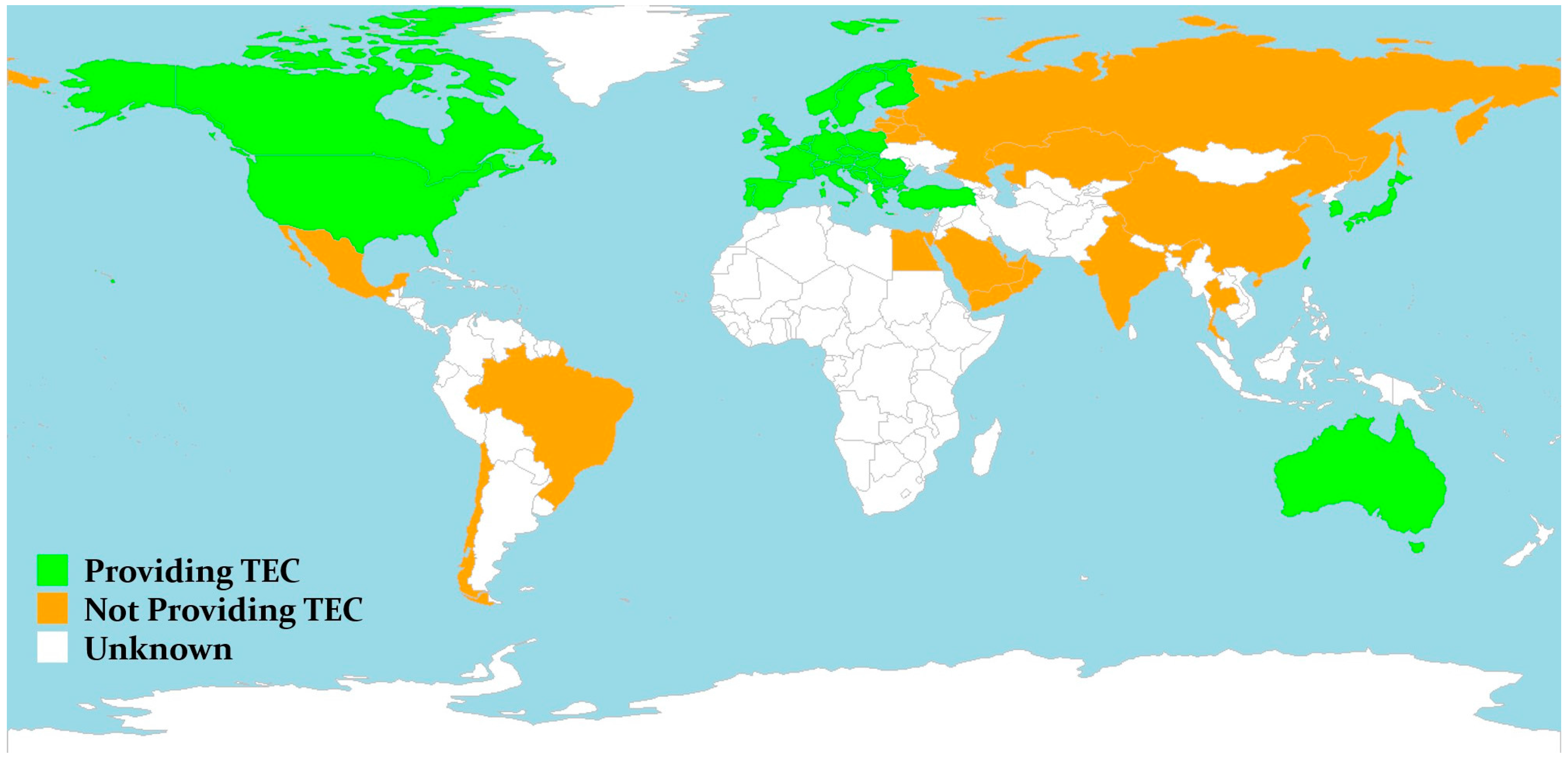
4.2. Worldwide Practices on Time Error Correction

Apart from three interconnection systems in North America, other interconnection systems around the world are also providing TEC services at this time. Figure 10 presents an illustrative example of the TEC process in the Japanese Western Interconnection system. Figure 10a gives the change of time error over one month. From Figure 10a, it can be observed that Japanese utilities also provide the TEC service similar to that of North American utilities. Once the accumulative time error has reached a predefined value, TEC services start working to cancel out this time error. However, it seems that compared with North American utilities, the threshold to start TEC service is set to be a low value in Japanese utilities, usually 6–7 s. Another observation is that Japanese utilities provide TEC services more frequently than North American utilities. According to the time error distribution depicted in Figure 10b, the maximum time error is about +7.59 s, the minimum time error is nearly −6.75 s, and the average time error is close to zero. Thus, the synchronous electric clock using power line frequency could likely run very well in Japan.

On the other hand, we also find that there are some Interconnection systems not providing TEC services for synchronous electric clocks. An illustrative example is the Brazil Interconnection system, as shown in Figure 11. From Figure 11a, it can be observed that the time error kept going up over this month. TEC services usually cause to a continuous decrease of the accumulative time error. However, such phenomenon was never found in Figure 11a of Brazil Interconnection system. Finally, the time error accumulated to a significant value (+80.39 s). The above observation is also confirmed by the probability distribution of power grid frequency shown in Figure 11b. From Figure 11b, it can be seen that power grid frequency follows the normal distribution very well. But, the mean frequency is 2 mHz higher than the nominal frequency (60 Hz). This deviation is the main reason why the clock finally accumulated to a large time error at the end of one month. Thus, the synchronous clock in Brazil would very likely have a big time drift in the long term.

Using the frequency measurements collected by worldwide FDRs in FNET/GridEye, we analyze the TEC practice around the world and identify regions of the world where electric utilities provide TEC services from those without TEC services according to measurements collected in 2016. In this study, if the average time error (absolute value) over one typical month of 2016 is larger than 10.00 s, this interconnection system would be considered to not provide TEC services. Otherwise, it would be considered to provide TEC services. Figure 12 demonstrates the identification result of TEC practices around the world. From Figure 12, it can be observed that the countries providing TEC services are concentrated in North America and Europe. In Asia and South America, however, most countries do not provide TEC services. Therefore, synchronous electric clocks installed in these countries usually tend to have a large time drift in the long term.

5. Power System Frequency Distribution Pattern Analysis

As discussed above, the long-term average of power grid frequency has great influence on the accumulative time error of synchronous electric clocks. Specifically, as demonstrated in Figure 11b, the monthly average frequency higher than the nominal value by only 2 mHz could eventually lead to a significant time drift (+80.39 s) at the end of one month. On the other hand, according to Equations (1) and (2), if the accumulative time error $\mathsf{∆}T$ is forced to be zero, the following equation can be derived

$$\overline{f}=\frac{1}{T}{\displaystyle \sum }_{t=1}^T{f}_t=f^{*},$$

(3)

where $\overline{f}$ is the long-term average of system frequency and $f^{*}$ is the nominal frequency. As shown by Equation (3), a necessary condition for the accumulative time error being zero is that the long-term average frequency should be equal to the nominal frequency. Therefore, it is believed that the long-term average of power grid frequency and its distribution pattern is also very valuable for statistical analysis of the time error. To do so, power system frequency distribution patterns are studied in this section and the differences between countries providing and not providing TEC services are also compared.

Figure 13 presents the probability density function (PDF) of power grid frequency in countries providing TEC services. The PDF curve is depicted by the kernel density estimator [30,31] using the frequency measurements of one year (2016). From Figure 13, it can be observed that the yearly PDF curve appears to be a standard normal distribution [32]. Another observation is that different interconnection systems have different frequency deviations. EI, WECC, ERCOT and European systems have very small frequency deviations (from −0.05 Hz to 0.05 Hz). As shown in Figure 13, although the frequency distribution pattern varies for these countries providing TEC services, their average frequency deviations (shown by numbers in brackets) are all less than ±0.10 mHz. Thus, the synchronous clock using power grid frequency in these countries could likely run very well in the long term.

Figure 14 shows the yearly PDF curves of power grid frequency in countries not providing TEC services. The yearly PDF curves of Russia and Brazil are close to standard normal distributions. On the contrary, the PDF curve of China looks like a saddle (a roughly bimodal distribution), which may be caused by the dead-band of governors [32]. For the three systems shown in Figure 14, their frequency deviations are all very small and usually vary from −0.05 Hz to 0.05 Hz. However, compared with the countries shown in Figure 13, the average frequency deviations are all very large in these countries not providing TEC services. Then, frequency deviations gradually accumulate over time and finally cause a big time drift of synchronous clocks in the long term.

6. Conclusions

In this paper, we used the power grid frequency measurements coming from the wide-area frequency monitoring network FNET/GridEye to carry out statistical analysis on the time error of synchronous electric clock. The time error correction (TEC) service provided by electric utilities was investigated and then the worldwide power system practices on TEC services were analyzed. The regions of the world where electric utilities provide TEC services are identified from those without TEC services. The following conclusions can be drawn from the analytical results.

Firstly, the synchronous clock using power line frequency as its timing source usually run very well if utilities provide TEC services. Secondly, in order to periodically remove the accumulative time error, many electric utilities around the world are providing the TEC service through offsetting the scheduled frequency by a small number. Thirdly, according to frequency measurements in 2016, analytical results present that the countries providing TEC services are concentrated in North America and Europe. In Asia and South America, however, most countries do not provide TEC services. Finally, the TEC service provided by electric utilities contributes to maintain the long-term average grid frequency at its nominal value. However, for the countries not providing TEC services, their long-term average frequency usually has a significant deviation from the nominal frequency.

References

1. Welch, K.F. The History of Clocks and Watches; Drake Publishers: Cardiff, UK, 1972. [Google Scholar]
2. Wise, S.J. Electric Clocks: Principles, Construction, Operation, Installation and Repair of Mains and Battery-Operated Clocks, 2nd ed.; Heywood: London, UK, 1951. [Google Scholar]
3. Thomson, A. The first electric clock. In Gold Bulletin; Springer: Berlin, Germany, 1972; Volume 5, pp. 65–66. [Google Scholar]
4. Lines, M.A. Ferranti Synchronous Electric Clocks; Electric Clocks: London, UK, 2012. [Google Scholar]
5. Hardis, J.E.; Fonville, B.; Matsakis, D. Time and frequency from electrical power lines. In Proceedings of the 48th Annual Precise Time and Time Interval Systems and Applications Meeting, Monterey, CA, USA, 30–31 January 2017; pp. 372–386. [Google Scholar]
6. Abdulraheem, B.S.; Gan, C.K. Power system frequency stability and control: Survey. Int. J. Appl. Eng. Res. 2016, 11, 5688–5695. [Google Scholar]
7. RG-CE System Protection & Dynamics Sub Group. Frequency Stability Evaluation Criteria for the Synchronous Zone of Continental Europe; ENTSO-E: Brussels, Belgium, 2016. [Google Scholar]
8. Amjady, N.; Fallahi, F. Determination of frequency stability border of power system to set the thresholds of under frequency load shedding relays. Energy Convers. Manag. 2010, 51, 1864–1872. [Google Scholar] [CrossRef]
9. Delassi, A.; Arif, S.; Mokrani, L. Frequency stability enhancement in power system using high-order sliding mode control. In Proceedings of the 4th International Conference on Electrical Engineering (ICEE), Boumerdes, Algeria, 13–15 December 2015; pp. 1–4. [Google Scholar]
10. Kiaee, M.; Cruden, A.; Infield, D.; Chladek, P. Improvement of power system frequency stability using alkaline electrolysis plants. Proc. Inst. Mech. Eng. Part A J. Power Energy 2013, 227, 115–123. [Google Scholar] [CrossRef]
11. Abdlrahem, A.; Venayagamoorthy, G.K.; Corzine, K.A. Frequency stability and control of a power system with large PV plants using PMU information. In Proceedings of the North American Power Symposium (NAPS), Manhattan, KS, USA, 22–24 September 2013; pp. 1–6. [Google Scholar]
12. Erlich, I.; Rensch, K.; Shewarega, F. Impact of large wind power generation on frequency stability. In Proceedings of the IEEE Power Engineering Society General Meeting, Montreal, QC, Canada, 18–22 June 2006; pp. 1–8. [Google Scholar]
13. Wang, Z.; Wu, K.; Guo, L.; Liu, W.; Cui, W. Impact of wind speed disturbance on power system frequency stability. In Proceedings of the IEEE Innovative Smart Grid Technologies-Asia (ISGT Asia), Kuala Lumpur, Malaysia, 20–23 May 2014; pp. 349–353. [Google Scholar]
14. Kundur, P.; Paserba, J.; Ajjarapu, V.; Andersson, G.; Bose, A.; Canizares, C.; Hatziargyriou, N.; Hill, D.; Stankovic, A.; Taylor, C. Definition and classification of power system stability. IEEE Trans. Power Syst. 2004, 19, 1387–1401. [Google Scholar]
15. Zhong, Z.; Xu, C.; Billian, B.J.; Zhang, L.; Tsai, S.J.; Conners, R.W.; Centeno, V.A.; Phadke, A.G.; Liu, Y. Power system frequency monitoring network (FNET) implementation. IEEE Trans. Power Syst. 2005, 20, 1914–1921. [Google Scholar] [CrossRef]
16. Zhang, Y.; Markham, P.; Xia, T.; Chen, L.; Ye, Y.; Wu, Z.; Yuan, Z.; Wang, L.; Bank, J.; Burgett, J. Wide-area frequency monitoring network (FNET) architecture and applications. IEEE Trans. Smart Grid 2010, 1, 159–167. [Google Scholar] [CrossRef]
17. Liu, Y.; You, S.; Yao, W.; Cui, Y.; Wu, L.; Zhou, D.; Zhao, J.; Liu, H.; Liu, Y. A Distribution Level Wide Area Monitoring System for the Electric Power Grid–FNET/GridEye. IEEE Access 2017, 5, 2329–2338. [Google Scholar] [CrossRef]
18. Xia, T.; Zhang, H.; Gardner, R.; Bank, J.; Dong, J.; Zuo, J.; Liu, Y.; Beard, L.; Hirsch, P.; Zhang, G. Wide-area frequency based event location estimation. In Proceedings of the IEEE Power Engineering Society General Meeting, Tampa, FL, USA, 24–28 June 2007; pp. 1–7. [Google Scholar]
19. You, S.; Guo, J.; Kou, G.; Liu, Y.; Liu, Y. Oscillation mode identification based on wide-area ambient measurements using multivariate empirical mode decomposition. Electr. Power Syst. Res. 2016, 134, 158–166. [Google Scholar] [CrossRef]
20. Liu, H.; Zhu, L.; Pan, Z.; Bai, F.; Liu, Y.; Liu, Y.; Patel, M.; Farantatos, E.; Bhatt, N. ARMAX-based transfer function model identification using wide-area measurement for adaptive and coordinated damping control. IEEE Trans. Smart Grid 2015, 8, 1105–1115. [Google Scholar] [CrossRef]
21. Liu, Y.; Zhan, L.; Zhang, Y.; Markham, P.N.; Zhou, D.; Guo, J.; Lei, Y.; Kou, G.; Yao, W.; Chai, J. Wide-area-measurement system development at the distribution level: An FNET/GridEye example. IEEE Trans. Power Deliv. 2016, 31, 721–731. [Google Scholar] [CrossRef]
22. Zhan, L.; Liu, Y.; Culliss, J.; Zhao, J.; Liu, Y. Dynamic single-phase synchronized phase and frequency estimation at the distribution level. IEEE Trans. Smart Grid 2015, 6, 2013–2022. [Google Scholar] [CrossRef]
23. Yao, W.; Liu, Y.; Zhou, D.; Pan, Z.; Zhao, J.; Till, M.; Zhu, L.; Zhan, L.; Tang, Q.; Liu, Y. Impact of GPS signal loss and its mitigation in power system synchronized measurement devices. IEEE Trans. Smart Grid 2017. [Google Scholar] [CrossRef]
24. Liu, Y.; Yao, W.; Zhou, D.; Wu, L.; You, S.; Liu, H.; Zhan, L.; Zhao, J.; Lu, H.; Gao, W. Recent developments of FNET/GridEye—A situational awareness tool for smart grid. CSEE J. Power Energy Syst. 2016, 2, 19–27. [Google Scholar] [CrossRef]
25. Wiser, R.; Bolinger, M.; Heath, G.; Keyser, D.; Lantz, E.; Macknick, J.; Mai, T.; Millstein, D. Long-term implications of sustained wind power growth in the United States: Potential benefits and secondary impacts. Appl. Energy 2016, 179, 146–158. [Google Scholar] [CrossRef]
26. U.S. Energy Information Administration (EIA). Electric Power Monthly; U.S. Department of Energy (DoE): Washington, DC, USA, 2017.
27. Zhang, Y.; Wang, J.; Zeng, B.; Hu, Z. Chance-Constrained Two-Stage Unit Commitment under Uncertain Load and Wind Power Output Using Bilinear Benders Decomposition. IEEE Trans. Power Syst. 2017. [Google Scholar] [CrossRef]
28. Operating Committee. Time Error Correction and Reliability White Paper; North American Electric Reliability Corporation (NERC): Atlanta, GA, USA, 2015; pp. 1–16. [Google Scholar]
29. North American Energy Standards Board (NAESB). Time Error Correction Standard; North American Energy Standards Board (NAESB): Houston, TX, USA, 2007. [Google Scholar]
30. Zhang, Y.; Wang, J. K-nearest neighbors and a kernel density estimator for GEFCom2014 probabilistic wind power forecasting. Int. J. Forecast. 2016, 32, 1074–1080. [Google Scholar] [CrossRef]
31. Wand, M.P.; Jones, M.C. Kernel Smoothing; Taylor & Francis: New York, NY, USA, 1994. [Google Scholar]
32. Markham, P.N.; Zhang, Y.; Guo, J.; Liu, Y.; Bilke, T.; Bertagnolli, D. Analysis of frequency extrema in the Eastern and Western Interconnections, 2010–2011. In Proceedings of the IEEE Power and Energy Society General Meeting, San Diego, CA, USA, 22–26 July 2012; pp. 1–8. [Google Scholar]
Figure 1. FNET/GridEye sensor deployment in North America. The red point shows the frequency disturbance recorder (FDR) location.
Energies 10 01283 g001
Figure 2. FNET/GridEye sensor deployment around the world. The colorful region indicates the area monitored by FNET/GridEye.
Energies 10 01283 g002
Figure 3. Time error change over one month in Eastern Interconnection (EI) system of North America. (a) Time-series curve of time error in October 2016; (b) Probabilistic distribution function of time error in one month. The blue color presents the fast time error. The orange color indicates the slow time error. The grey line shows the estimated probability density of time error.
Energies 10 01283 g003
Figure 4. Time error change over one month in Western Electricity Coordinating Council (WECC) of North America. (a) Time-series curve of time error in October 2016; (b) Probabilistic distribution function of time error in one month. The blue color presents the fast time error. The orange color indicates the slow time error. The grey line shows the estimated probability density of time error.
Energies 10 01283 g004
Figure 5. Time error change over one month in Electric Reliability Council of Texas (ERCOT) system of North America. (a) Time-series curve of the time error in October 2016; (b) Probabilistic distribution function of time error over one month. The blue color indicates the fast time error. The orange color presents the slow time error. The grey line shows the estimated probability density of time error.
Energies 10 01283 g005
Figure 6. Monthly change of the time error for Eastern Interconnection (EI) system of North America from 2014 to 2017. The blue bar shows the maximum time error (positive value, i.e., running fast time error) in this month. The orange bar presents the minimum time error (negative value, i.e., running slow time error) in this month. The grey line indicates the average time error over one month.
Energies 10 01283 g006
Figure 7. Yearly change of the time error for Electric Reliability Council of Texas (ERCOT) system of North America from 2008 to 2017. One typical month is selected to represent every year. The box-plot depicts the maximum and minimum time error (the ends of the whiskers), the first and third quartiles (the bottom and top of the box), and the mean time error (the band inside the box).
Energies 10 01283 g007
Figure 8. Illustrative example of fast time error correction (TEC) process in Eastern Interconnection (EI) system of North America: (a) Time error change from 24 October 2016 07:00 a.m. to 25 October 2016 01:00 p.m.; (b) Power system frequency change during the same period of (a). The grey vertical line indicates the starting/stopping point of the TEC process. The red solid line indicates the average system frequency before, during and after the TEC process.
Energies 10 01283 g008
Figure 9. Illustrative example of slow time error correction (TEC) process in Eastern Interconnection (EI) system of North America: (a) Time error change from 10 May 2015 07:00 p.m. to 11 May 2015 07:00 p.m.; (b) Power system frequency change during the same period of (a). The grey vertical line indicates the starting/stopping point of the TEC process. The red solid line indicates the average system frequency before, during and after the TEC process.
Energies 10 01283 g009
Figure 10. Time error change over one month in Karuizawa, Janpa. (a) Time-series curve of time error in October 2016; (b) Probabilistic distribution function of time error in one month. The blue color presents the fast time error. The orange color indicates the slow time error. The grey line shows the estimated probability density of time error.
Energies 10 01283 g010
Figure 11. Time error change over one month in Itajubá, Brazil. (a) Time-series curve of time error in October 2016; (b) Probabilistic distribution function of the system frequency in one month. The blue color presents the fast time error. The orange color indicates the slow time error. The grey line shows the estimated probability density of power grid frequency. The vertical dashed line presents the average frequency of this month.
Energies 10 01283 g011
Figure 12. Time error correction (TEC) practice around the world. The green region indicates the countries providing TEC service. The orange region indicates the countries not providing TEC service.
Energies 10 01283 g012
Figure 13. Probability distribution of power system frequency in countries providing the time error correction in 2016. (a) Three major interconnection systems in North America; (b) Interconnection systems around the world. Figures in brackets denote the average frequency deviation away from the nominal frequency.
Energies 10 01283 g013
Figure 14. Probability distribution of power system frequency in countries not providing the time error correction in 2016. Figures in brackets denote the average frequency deviation away from the nominal frequency.
Energies 10 01283 g014