A Novel Hybrid Approach for Numerical Modeling of the Nucleating Flow in Laval Nozzle and Transonic Steam Turbine Blades


Department of Mechanical Engineering, Ferdowsi University of Mashhad, Mashhad 9177948974, Iran
*
Author to whom correspondence should be addressed.
Energies 2017, 10(9), 1285; https://doi.org/10.3390/en10091285
Submission received: 13 May 2017
/
Revised: 16 August 2017
/
Accepted: 21 August 2017
/
Published: 29 August 2017
(This article belongs to the Section I: Energy Fundamentals and Conversion)
Abstract
:In the present research, considering the importance of desirable steam turbine design, improvement of numerical modeling of steam two-phase flows in convergent and divergent channels and the blades of transonic steam turbines has been targeted. The first novelty of this research is the innovative use of combined Convective Upstream Pressure Splitting (CUSP) and scalar methods to update the flow properties at each calculation point. In other words, each property (density, temperature, pressure and velocity) at each calculation point can be computed from either the CUSP or scalar method, depending on the least deviation criterion. For this reason this innovative method is named “hybrid method”. The next novelty of this research is the use of an inverse method alongside the proposed hybrid method to find the amount of the important parameter in the CUSP method, which is herein referred to as “CUSP’s convergence parameter”. Using a relatively simple computational grid, firstly, five cases with similar conditions to those of the main cases under study in this research with available experimental data were used to obtain the value of z by the Levenberg-Marquardt inverse method. With this innovation, first, an optimum value of was obtained using the inverse method and then directly used for the main cases considered in the research. Given that the aim is to investigate the two-dimensional, steady state, inviscid and adiabatic modeling of steam nucleating flows in three different nozzle and turbine blade geometries, flow simulation was performed using a relatively simple mesh and the innovative proposed hybrid method (scalar + CUSP, with the desired value of ). A comparison between the results of the hybrid modeling of the three main cases with experimental data showed a very good agreement, even within shock zones, including the condensation shock region, revealing the efficiency of this numerical modeling method innovation. The main factor in improving the aforementioned results was found to be a reduction of the numerical errors by up to 70% in comparison to conventional methods (scalar, Jameson original), so that the mass flow rate is well conserved, thereby proving better satisfaction of the conservation laws. It should be noted that by using this innovative hybrid method, one can take advantages of both central difference scheme and upstream scheme (scalar and CUSP, respectively) at the same time in simulating complex flows in any other finite volume scheme.
1. Introduction
Efficiency enhancement of steam turbines, which are important components of the power generation industry, has been always considered by designers. In these plants, for low pressure transonic turbines, the droplet formation becomes significantly important. Finite volume numerical methods are conventionally used to predict the two-phase flow behavior in these steam turbines [1,2,3]. Considering the liquid-vapor two-phase phenomena governing the flow, and also considering the presence of blades of tip-section geometry, given the relatively high complexities, there is still a need for improved numerical methods with reduced numerical errors, for accurate modeling of the flow. For this purpose, one may see the derivation of a more accurate numerical method to capture condensation shock and aerodynamic shocks (flow discontinuities) with minimum fluctuations and, particularly, minimal numerical errors as one of the important challenges faced by computational fluid dynamics (CFD) [4,5,6,7].
Vapor flow through the nozzles and cascade blades in the low pressure transonic steam turbine is transformed into supercooled steam due to the rapid expansion and delay in fluid condensation. The phase change of the fluid from vapor to liquid droplets results in the release of some latent heat, part of which will be stored in the droplet, thereby, increasing it’s temperature. This effect in nucleation zone results in local increase in pressure (or what is referred to as condensation shock), thereby reducing the turbine’s performance [8,9]. Bakhtar and Tochai [10] were the first to propose a two-dimensional solution for the two-phase vapor flow between steam turbine blades using Denton’s finite-volume method. Then, looking for better solutions, they applied a Runge Kutta algorithm developed by Jameson, which was of second-order precision in space, for an expansive inviscid flow, and showed that the Jameson method offers better capabilities in terms of shock capturing in two-phase steam flows [11,12].
Only a limited number of numerical methods are capable of modeling complicated two-phase phenomena in relatively complex geometries. Since this flow begins nucleation at a considerable rate under non-equilibrium conditions within the Wilson pressure range [1,7,13], a Lagrangian approach along with a standard H-grid are often recommended for calculating droplet growth in two-phase flows because of non-simplicity in convergence, and complexity of the flow [2,7,14,15]. Several credible papers [1,12,16,17,18] have proved that this grid is independent of the finite volume solution for the test cases used in the present research. In this research, in order to calculate the nucleation of new droplets, the modified classical nucleation equation by Courtney and Kantrovitz [9,15,18] is used, while the droplet growth is determined by a Lagrangian solution in the proposed novel hybrid numerical approach, which will be explained in detail in the following sections. Furthermore, the expansive nature of the flow through nozzles and turbines, which results in a thin boundary layer, allows one to assume the flow as being inviscid [1,7,12,19,20].
Since difference-based methods can be divided into two groups, namely central difference schemes with dissipation scheme and upstream schemes, one group of solutions for Euler equations are based on the propagative characteristic of waves; this group of methods are referred to as upstream flow schemes. The direction of discretization of the differential equations and data acquisition is in harmony with the behavior of the inviscid flow. From the 1980s onwards, extensive attempts have been focused on modelling and adopting upstream flow schemes; these attempts are classified under two general classes, namely flux vector splitting methods and flux difference splitting methods which use propagative characteristic of wave to solve Euler equations. The common point in these two classes of methods lies in the relationship between the amplitude propagation direction, the direction along which the differential equations are expanded, and synchronization of solution domain with flow behavior [21].
In 1995, Jameson [22] was among the first to establish the basis of the discretization schemes of the past two decades. He presented an Upstream Pressure Splitting scheme, named CUSP, as an advanced analytical scheme for compressible flows. In this form of artificial dissipation, there are a combination of second-order and fourth-order dissipation terms which have been used by numerous researchers. This scheme is based on the assumption that, fourth-order artificial dissipation terms across the entire area are considered firstly, and then, added to prevent nonlinear instabilities. The CUSP method [23] belongs to a group of schemes proposed based on Flux Vector Splitting along with governing pressure flux. In 2015, Folkner et al. [24] performed flow modeling on airfoils with a focus on the importance of adjusting low Mach numbers in steady state and also modeling in unsteady state, using the CUSP numerical method. They further compared the obtained results against those obtained when a matrix dissipation scheme was used, and the superiority of the CUSP method was evident with reference to experimental data. Another approach to increase model accuracy is to use the Levenberg-Marquardt inverse method to achieve results of adequate accuracy in shorter times than those of conventional solutions [25,26]. The Levenberg-Marquardt algorithm is used to find the minimum of a multivariate nonlinear function; it is designed as a standard method for solving least squares problems for nonlinear functions, and exhibits high efficiency in solving inverse engineering problems. As of present, this algorithm can be used to solve a variety of nonlinear equations [27].
In the present research, in order to reduce numerical errors and thereby improve the results, application of an improved CUSP scheme in Jameson’s two-dimensional finite volume method has been investigated, which is in continuation of previous research and publications of the authors [6,16,17]. The first novelty of this research is the innovative combined use with CUSP and scalar methods (hereforth referred to as the hybrid method) to update the properties at each calculation point. In other words, each property (, , and ) at each calculation point can be calculated by either a CUSP or scalar method, depending on the least deviation (between two latest iterations) as a criterion, but when it comes to the whole set of the aforementioned properties at each calculation point, both of these methods may be used. This is why this innovative method is called the hybrid method.
The next novelty of this research is the use of an inverse method with the proposed hybrid method to find an optimum value for the important parameter z in the CUSP method, which is herein referred to as the “CUSP convergence parameter”. Accordingly, first, five cases of similar conditions to with those of the main cases under study in this research but with available experimental data were used to obtain the value of CUSP’s convergence parameter, , by using Levenberg-Marquardt’s inverse method. With this innovation, first, the correct optimum value of is obtained, so that the inverse method is no longer required for determining the z parameter for the main test cases. The obtained value is then directly used for the main cases considered in the research within the framework of the proposed hybrid method. The experimental data of the main cases are used to validate the innovative hybrid modeling results.
As mentioned before, the aim in this research is to improve two-dimensional modeling of steady state and adiabatic steam nucleating flows in three different geometries (namely Young nozzle type L, mid-section turbine blade, and relatively complicated geometry of tip-section blade of the steam turbine), which is performed using a relatively simple computational grid and the proposed innovative hybrid method (scalar + CUSP, with the desired value of ). Afterwards, a comparison is made between the results of the proposed hybrid modeling in the mentioned cases and experimental data, with an emphasis on shock zones, including the condensation zone. It should be noted that using this innovative hybrid method, one can take advantage of both the central difference scheme and upstream scheme (scalar and CUSP, respectively) at the same time in simulating complex flows in any other finite volume schemes.
2. Two-Phase Flow
One of the attributes of steam flow in turbine blade passageways is it’s rapid expansion and diversion from thermodynamic equilibrium, where without any liquid formation, in supercooled or supersaturated vapor conditions, the gas can expand until the Wilson line in Mollier’s diagram. In this situation, return to equilibrium happens through spontaneous water droplet formation and growth [19,28,29]. In this research, droplet growth is modeled following a Lagrangian solution and Eulerian method for gas phase analysis done using a finite volume method. Due to the formation of condensed flow, modeling the steam turbine cascades is much more complex than dry flow conditions. The droplets which form and grow in homogeneous flow due to sudden condensation in turbine blade passages are minuscule and normally have a radius smaller than micron-order, and in this situation, due to the small size of the droplets the velocity difference or drag force between the vapor phase and droplets can be neglected [1,2,9,16,20].
2.1. Conservation Equations Governing the Main Flow
The conservation equations governing the main gas flow which is two-phase, compressible, adiabatic, steady state and inviscid, are expressed by Equations (1) and (2):
where the vector contains the flow conservation variables, vectorsexpress inviscid fluxes, is the total energy, is the total enthalpy and are components of velocity. Due to the flow being expansive in the nozzles and turbines which results in a boundary layer with low thickness, the flow is assumed to be inviscid [1,9,12,15].
2.1.1. Equation of State
The equation of state for the gas phase must be compatible with the equations used for obtaining it’s thermodynamic properties, and the vapor phase to be non-equilibrium near the saturation line especially supercooled vapor, but acceptably accurate inside the saturated region. Accordingly, the virial equations of state suggested by Vokalovich [7,18,30] is adopted in Equation (3). To reduce the calculation load, and considering sufficient accuracy, the first virial coefficient based on [1,7,12,30] is set as:
where the subscripts refer to the steam phase. In Equation (3) , and are density, temperature and vapor gas constant respectively, and is the first virial coefficient. The steam table in reference [31] is used for calculating the liquid phase thermodynamic properties.
2.1.2. Wetness Fraction
In condensing flows, the most important impact of phase change is defined by the release of the latent heat. To investigate this phenomenon and to implement the effects of the two-phase flow, a wetness fraction parameter needs to be inserted into the main equations. Other required data for expressing the fluids properties for the gas and liquid phases are extracted from Keenan and co-worker’s equations [31]. Using the following nucleation equation, the number of new droplets produced in each calculating element is calculated. The total number of droplets at the outlet of each calculating element (N), includes the number of droplets in the previous elements plus the number of new droplets. So In each calculation element, the wetness fraction, , is practically calculated from the droplet’s radius, r, and number of droplets, N, at the outlet of the element:
where the subscript refers to the liquid phase.
2.1.3. Nucleation Equation for the Critical Radius
The number of critical droplets during each step produced by the nucleation process can be calculated by knowing the modified classical nucleation rate, the fluid’s solution stage travel time () and the volume of the element as shown by Equations (5) and (6) [1,7,9,13,15,32]:
where is the improved classical nucleation rate, is the element volume, is the condensation coefficient, is the correction factor in the nucleation equation, is Gibbs energy and is Boltzmann’s constant and is the flat Surface tension for water which is obtained from Steam Tables [31].
2.1.4. Relations of Droplet Growth
The droplet growth rate is calculated based on the heat transfer process and mass transfer between the droplets and vapor in different flow regimes in the passage and it should be noted that the mentioned heat transfer depends on the unknown temperature of the droplet, . In this research, the droplets temperature is obtained using Gyarmathy’s approximation [1,7,19,33] and also, to further reduce of the volume of calculations for Equation (9a) only in the wet region (or relative equilibrium condition), a direct approximation is used, as introduced by Equation (9b) [1,9,12,19]:
where is steam saturate temperature, is latent heat, is heat transfer coefficient of droplet with surrounding vapor, is the Knudsen number, is the mean free path of a vapor molecule, is inlet radius element and is Thermal conductivity.
Indeed, it should be noted that after the completion of nucleation, new droplets are no longer formed and the size of the droplets are calculated using Equation (9a) similar to the droplet growth in the nucleation region, and using Gyarmathy’s equation, the droplet’s temperature is simultaneously specified. The droplet radius averaging approach in the nucleation region and beyond is explained in the following two conditions:
- (a)
- The number of produced droplets and the average radius at the inlet of the new calculation element is defined by the average radius at the outlet of the previous element. In the nucleation region, the number of new droplets and their radius is determined in the new calculation element. Both new and old sets of droplets can grow along the calculation element, knowing the number of droplets in each of the sets, different methods including surface or volume averaging can be used to calculate the average radius at the outlet of the new calculation element.
- (b)
- In the region after the nucleation, i.e. the wet region, the flow tends towards equilibrium or saturation, the number of droplets is constant and the droplets can only grow. After calculating the droplet growth in each calculation element, any of the mentioned averaging methods can be used to obtain the average radius, which in this research, to reduce the calculations the surface averaging method is used.
3. CUSP’s Method
The basis of this method is separation of the pressure terms in the flow flux equations [23]. In these methods, the flux on the side of each element is partitioned into convective and pressure portions, and for calculating the displacement fluxes the upstream flow approximation and for the pressure portion, the upstream approximation is used considering the acoustics, which is determined by it’s amount and sign at two directions of each side. In the two dimensional case, the flux vector is partitioned into pressure and convective fluxes which are composed of two components in the and directions, and are expressed by Equations (10)–(12) [34]:
In the above equations, and are the surface borders in the and directions (see Figure 1) and is the enthalpy. which includes the flow conservation variables in 2D conditions is expressed by Equation (13):
In Equation (14), the components of the flow flux are partitioned into displacement and pressure parts where:
Considering the convective flux, , for the Equations (15)–(17) are obtained for the pressure flux terms:
To obtain more accurate results, artificial dissipation loss terms with high values in regions close to impact waves, and low values in other regions of the solution space must be entered in the solutions. For this purpose, a switch function which is capable of flow detection and has an important role in the convergence of the solution is entered in the calculations [23]. In the first step, the initial flow variable vector at right and left hand sides of and , is calculated with the help of the switch function which is defined in Equation (18) [16,21,23]:
The value of the power which in this research is named the “CUSP convergence parameter”, is selective and is considered to be between 2 and 3. Furthermore, for , a value between 1 to 5 is suggested. Equation (18b) is recommended for modeling in very low velocities such as modeling free convection heat transfer, since the fraction will show its effect [21]. Moreover, research has shown that Equation (18a) is suitable for modeling the flow in the nozzle or between turbine blades [17].
4. Inverse Method
The aim of inverse modeling is to find the values for the unknown parameters (for example the value of ) using available experimental data. For ill-posed problems the direct and exact solution cannot be used for obtaining the unknown parameters. Therefore, finding the appropriate relation, fit between the measured values and direct solution which is explained in the following sections.
4.1 The Mathematics of the Problem
In the inverse problem, the error, , is defined as the difference between the measured output, , and the model’s outlet at the location of measurement, , [35]:
In this problem, and vectors are single units, because the result of the solution under steady state conditions and at one point of the solution space is considered, and these vectors are the experimentally measured pressures and calculated pressures at one specific region. In this research the goal is to compare these pressures, until we reach an appropriate combination of steady state conditions for mass conservation which includes the least changes of mass influx relative to the inlet mass influx in the simulation. It is to note that the pressure can be approximated using the solutions for similar cases. To minimize this error, there are different methods for defining the objective function. One conventional method is to use the square errors approach. In the inverse problem, the objective is to minimize the sum of squared errors and using specific weights, , the influence of each error can be changed [36]:
where is a function of variable . In this problem, vector has the dimensions of , ( is the number of variables in the matrix) where each of it’s elements represent the proportion of the upstream CUSP in the hybrid method (Scalar (Jameson) + CUSP), and the proportion of the Scalar finite volume method will be later defined in the program execution stage. Here, weights are not used in the calculations. Therefore, the Levenberg-Matquardt’s method for obtaining unknown parameters works as follows:
where is called the depreciation regulatory parameter and is a diagonal matrix as defined by Equation (22):
where the sensitivity matrix is defined as below. For inverse problems with linear behavior the sensitivity matrix is not a function of the unknown parameters as expressed by Equation (23) [35]:
Introduction of to the repeating equation, is for depreciating the oscillations and instabilities which appear due to the malign character of the problem. The depreciation parameter is normally large at the beginning of the simulation where the unknown parameter is selected based on a first guess, therefore following this approach, there is no need to investigate the singularity of the term .
4.2. Convergence of the Solution
Generally, for the conservation of stability in explicit schemes, the biggest time interval is determined using the Courant condition:
where is the quantity of velocity, , is the speed of sound and is the distance interval. is the Courant number which is reported to be for the standard fourth order Scalar (Jameson) and up to 0.4 will not cause any problems for the stability. In this research, change in the value of the axial velocity is considered as the convergence criterion in Equations (25) and (26) [1,12,16,18]:
To prevent high iterations for the Levenberg-Matquardt’s method, some criteria have been proposed by Denis which are shown in Equation (27) [37,38]:
where the terms , and are small numbers for convergence [35]. The conditions given by Equation (27) are tests for the minimum sum of squared errors which is considerably small, and it is expected that it finds the closest answer to the real solution [39], where by establishing convergence in Equations (25)–(27), the final index is selected.
In this research, first, the hybrid (scalar (Jameson) + CUSP) modeling approach will be followed to model two-phase steam flow for five nozzles with different geometries (Moore nozzle types A and B, Young nozzle type C, Barschdorff nozzle) and also the dry flow between the blades of a turbine with moderate slope. The numerical results and experimental data will be used to obtain the optimum value for the power z using an inverse technique. This optimization will be done using the Levenberg-Matquardt’s inverse method as explained in this paper, the power z in referred to as the “CUSP’s convergence parameter” and it’s optimum value is obtained through inverse modeling of the named test cases (which all have similar conditions to the main cases in this research). With this innovation, i.e., obtaining the optimum value of the convergence parameter , there is no need to perform inverse modeling, for the main study cases in this research and instead the experimental results are used for validating the proposed novel hybrid model.
5. Algorithm for Combining the Scalar and CUSP Finite Volume Methods with the Inverse Method
For the solution domain in the current research, the standard H mesh is used and with the selection of this simple grid as shown in the work of the authors [6,11,12,17,18] the complexities and volume of calculations are reduced to an extent. To accelerate reaching a steady solution in the two-phase condition, first, the model is run for dry conditions over the entire path of the nozzle or blade, and this solution is used as the first guess for the modeling of the two-phase flow. It is to note that the independence of solution from the calculation mesh is checked and proved for all cases, which for the sake of brevity is not described here.
The solution range process of this research is divided into three stages: single phase (dry steam), nucleation (start of two-phase) and two-phase (without new droplets). Based on the authors’ experience, the dry steam flow is run for a limited number of times, e.g. 10 runs for the scalar (Jameson) and then the CUSP is run for the same number of times. Then the results are passed onto the inverse method for analysis and finally every combination will be checked for the final convergence of Equations (25)–(27), and these procedures are conducted in order (Figure 2). In the second step of the flow solution, the equation for real gases alongside dry flow conditions are considered and procedures similar to step one are continued. In the third step, two-phase equations are used where scalar (Jameson) criterion along with CUSP and inverse criterion control the convergence of the solution domain.
Determining flow properties in the nucleation and the two-phase regions is dependent on the wetness fraction calculations. For this purpose, the main flow equations must be solved simultaneously with droplet formation and growth equations. One major difference between these two sets of mentioned equations is that the equations governing droplet formation and growth are more sensitive to time and have to be integrated on smaller time intervals. Although the flow equations are based on the Eulerian viewpoint, the droplet growth equations naturally have a Lagrangian form, and for this reason, it is assumed that the droplet growth is calculated along the flow stream lines.
In the following sections, the novel hybrid scalar and CUSP method is used for the first time to model the steam two-phase gas liquid flow between the Laval nozzle, mid and tip-section blades of a steam turbine (Young nozzle type L, mid-section turbine blade, tip-section turbine blade). As described, after demonstrating the independence of the computational grid from the solution, initial values are assigned to the solution domain, and using the optimum value for the convergence parameter which is obtained through inverse modeling of similar cases. For the second step, a limited number of iterations, which based on the experience of the authors, can be 10 runs, is performed for the scalar (Jameson) and then the same number of runs is conducted for the CUSP method (and employing the nucleation and droplet growth equations for both methods for two-phase region). Then, the latest outputs from the scalar and CUSP methods (for example runs 9 and 10) are compared and those properties (parameters) which show less deviation from run 9 are stored (a matrix is used for this purpose). It is to note that the thermodynamic properties () and a velocity parameter () are four parameters which are updated from the flow governing equations. In this approach it is possible that the values of some of these parameters are updated from the scalar method and the rest from CUSP. Therefore, in each computational point, depending on the selection criterion which is shown in Figure 3, the updated values of all four parameters may neither be scalar nor CUPS methods, but rather from a combination of them. With defining new data, the solution domain will be investigated by the two convergence parameters of CUSP and scalar to satisfy the conservation of mass flow rate. This procedure repeats until final convergence is reached.
6. Results
The steam nucleation flow is considered and modeled as an adiabatic, steady state, 2D and two-phase flow. To obtain the optimum convergence parameter , first, the novel hybrid method (scalar (Jameson) + CUSP) is used alongside the inverse method for different geometrical cases with steam two-phase nucleating condition which are similar to the main cases investigated in this study, where the results of each case is explained in the following section. It is to note that all used cases have the required experimental data needed for inverse modeling. In the proposed approach the hybrid method involves numerical solutions of scalar, CUSP and the inverse method, and Figure 4, Figure 5, Figure 6, Figure 7, Figure 8, Figure 9, Figure 10, Figure 11, Figure 12, Figure 13, Figure 14, Figure 15 and Figure 16 show the geometry, static pressure to inlet stagnation pressure distribution and also the distribution of the logarithmic changes in the droplet radius along the central axis against experimental data (which is used for inverse modeling). Building on explanations given in previous sections, considering the small thickness of the boundary layer in expanding flows particularly in the investigated cases, the flow is assumed to be inviscid. Also due to the small diameter of the droplets, the drag force between the droplet and the vapor around it is neglected. For all the used cases, considering the passage geometry and other conditions, the independence of the solution from the calculation mesh is proven, but for the sake of brevity is not presented in the paper.
6.1. Moore Nozzle Type A
Figure 4 shows the geometry of the Moore nozzle type A [40], where the results of modeling performed by the scalar (original Jameson) finite volume method and the hybrid (scalar + CUSP + Inverse) method are compared with experimental data. In Figure 5 a drop of the pressure ratio is observed where, due to the condensation shock, the pressure ratio first increases until just after the nozzle’s throat, and then starts dropping because of nucleation ceasing and supersonic flow conditions. Figure 6 illustrates the logarithmic changes in droplet radius along the central axis of the nozzle. As shown in this figure, the changes of droplet radius at the beginning, where the supercooled degree is high, is rapid with a steep slope, but after the nucleation region has a slow growth and the flow relatively reaches equilibrium state. It should be noted that the difference between the radius calculated from theory is also reported in the results of other studies [2,41]. As mentioned, at this stage the aim of using inverse modeling is to obtain an optimum value for the parameter which will be calculated in the next section.
6.2. Moore Nozzle Type B
The geometry of the Moore nozzle type B [40] is depicted in Figure 7, where the results of modeling performed by the scalar and the hybrid (scalar + CUSP + Inverse) finite volume methods are compared with experimental data. Figure 8 shows the comparison for the static pressure to stagnation pressure ratio distribution and Figure 9 illustrates the logarithmic changes in droplet radius along the central axis of the nozzle, similar to the previous case. As mentioned, at this stage the aim of using inverse method is to obtain an optimum value for the parameter which will be calculated in the next pages.
6.3. Young Nozzle Type C
Figure 10 shows the geometry of the Young nozzle type C [42,43], where the results of modeling performed by the scalar (original Jameson) and the hybrid (scalar + CUSP + inverse) finite volume methods are compared with experimental data. Figure 11 shows the comparison for the static pressure to stagnation pressure ratio distribution along the central axis of the nozzle. As already mentioned, at this stage the aim of using inverse method is to study an optimum value for the parameter which will be calculated in the next pages.
6.4. Barschdorff Nozzle
The geometry of the Barschdorff nozzle [8,44] is shown in Figure 12, where the results of modeling performed by the scalar (original Jameson) and the hybrid (scalar + CUSP + inverse) finite volume methods are compared with experimental data. Figure 13 shows the comparison for the static pressure to stagnation pressure ratio distribution and Figure 14 illustrates the logarithmic changes in droplet radius along the central axis of the nozzle, similar to the previous cases. As already mentioned, at this stage the aim of using inverse method is to obtain an optimum value for the parameter which will be calculated in the next pages.
6.5. Mid-Section Turbine Blade
In continuation of applying the hybrid and inverse methods in modeling different nozzles for obtaining an optimum convergence parameter , the hybrid method is used for modeling single phase flow between the mid-section blades of a steam turbine. Figure 15 shows the standard computational mesh for mid-section turbine blades.
Due to the importance of the results on the suction surface, in Figure 16, the changes in static to stagnation pressure ratio along the length of the blade on the suction surface for dry flow, and also the impact of using CUSP’s method in the improved method are shown. As mentioned earlier, at this stage the aim of using inverse modeling is to investigate an optimum value for parameter which will be calculated in the next pages.
As explained, in this research, for obtaining the optimum convergence parameter , the hybrid (scalar + CUSP) method along with an inverse technique were used with experimental data for five laboratory cases (which are required for the inverse modeling for finding the optimum value of . Considering the improvements of the novel modeling in comparison with experimental data in the mentioned geometries, using Levenberg-Matquardt’s inverse method, the changes in the convergence parameter against improved changes of mass flow rate are calculated and shown in Figure 17.
Therefore, an average value of is found for the convergence parameter and can be used in Equations (18a) and (18b). Obtaining an average convergence parameter , for similar cases, (or three main cases) without performing inverse modeling, this average value can be used in the proposed hybrid (scalar + CUSP) method. In this case, there will be no need for experimental data, and if available, they can be used for validating the model. In other words, with this novelty, first, the optimum is obtained from similar cases, and then it is used directly in the proposed hybrid (scalar + CUSP) method (without performing again the inverse modeling) for simulating the complex flow.
In the research explained in the preceding sections, in the inverse method, instead of using the impact of weights (considering constant proportion/percentage for each method), the variable proportion of each method (scalar and CUSP) is calculated. Figure 18 shows the results of the inverse method for finding the best convergence parameter value by presenting the changes in the effective percentage of CUSP along the length of the blade. Using the effectiveness degree of the CUSP method in the hybrid method, the conservation of mass is satisfied with the least calculated error oscillations.
The main goal of this research is to model the steam two-phase gas-liquid flow in three different geometries (Young nozzle type L, turbine blade with average and steep slopes) using the hybrid (scalar (original Jameson) + CUSP) method. As explained in the previous sections, first, the desirable convergence parameter value is obtained from the similar cases, so there is no need for conducting inverse modeling in the proposed hybrid method for three main cases. The boundary conditions for three main case are as listed in Table 1.
The computational grid used, as explained in the Introduction, is a standard mesh, where the independence of the finite volume solution from the grid system is already proven in several works conducted by the authors and others [1,6,7,12,16,18] where of course, this dependence is also proven for the hybrid method. The reason for selecting this mesh is that we wanted to focus on the proposed hybrid (scalar + CUSP) method considering the more calculations needed for the two-phase flow in iterative methods. Therefore, the strength of the solution method (which in this research is the hybrid scalar and CUSP with the known optimum value of would be demonstrated using a standard computational mesh.
It is noteworthy that in all three mentioned geometries, after the convergence of the hybrid method, a limited number, e.g., 100 reiterations of CUSP (without combination with scalar) or even 100 reiterations of the scalar method (without CUSP) is continued, but due to the satisfaction of the conservation equations, no change is observed in the results.
6.6. Young Nozzle Type L
Figure 19 illustrates the geometry of the Young nozzle type L [10] and Figure 20, Figure 21, Figure 22, Figure 23, Figure 24 and Figure 25 show the improved modeling results using the steam two-phase scalar combined with the CUSP finite volume methods and incorporating the obtained optimum convergence parameter from similar cases () which is used for the first time for modeling Young nozzle type L in supersonic conditions.
Figure 20 shows the changes in static to inlet stagnation pressure ratio along the nozzle, where pressure ratio drop is observed until just after the nozzle’s throat, and due to the existence of condensation shock, first, there will be an increase in the pressure ratio, and then, because of nucleation halt and the flow being supersonic, this pressure ratio will follow a descending trend. Comparing the results of the proposed hybrid method (using ) with experimental data [10] shows improvement in the novel solution and indicates it’s obvious superiority.
In the conducted modeling, due to the adiabatic and inviscid flow, the stagnation pressure must remain constant until before the shock. To verify this, the changes of stagnation pressure to the initial nozzle inlet stagnation pressure for the two-phase flow is obtained from the two-phase hybrid (scalar + CUSP + ) and scalar finite volume methods for supersonic conditions and shown in Figure 21, where the smaller variations indicate closer agreement with initial pre-assumptions. Since in the proposed approach, stagnation pressure changes in adiabatic reversible regions is small, and also in the shock region and beyond it has about 60%, therefore, the results of this proposed improved hybrid method are closer to the assumptions and the flow reality.
The sudden condensation region is located after the throat and Figure 22 shows these changes in the wetness ratio resulting from the hybrid (scalar + CUSP) method and the numerical scalar method along the central line of the flow.
Since the Wilson point occurs after the throat, therefore nucleation has started, and Figure 23 shows the changes in the nucleation rate along the divergent section obtained from the two-phase hybrid (scalar + CUSP + ) in supersonic conditions after the throat.
Figure 24 also clearly shows the logarithmic changes of droplet radius along the nozzle in the central line. As shown in the figure, the changes in droplet radius at the beginning where the supercooled degree is high, is rapid with steep slope, but after the nucleation region will have a slow growth and the flow will reach relative equilibrium. In this modeling attempt, also, by comparing the results of the mentioned numerical methods with experimental data, the optimality of the hybrid method is shown.
Considering steady state conditions for the conservation of mass, the inlet mass flow rate along the path is constant. Figure 25 shows the percent change in mass flow rate, where by using the hybrid method, a relatively high improvement of about 70% is observed compared to the scalar without CUSP, which is a new accomplishment in better satisfying the mass conservation law, or better verification of the results.
6.7. Mid-Section Turbine Blade
Figure 15 shows the geometry for the mid-section turbine blade, where in this case modeling of the two-phase flow is conducted under different conditions. The obtained results from using the improved hybrid two-phase scalar and CUSP in conjunction with the optimum convergence parameter obtained from the similar cases () for modeling the mid-section turbine blades in supersonic conditions are shown in Figure 26, Figure 27, Figure 28, Figure 29, Figure 30, Figure 31 and Figure 32.
Figure 26 shows the changes in the static to stagnation pressure ratio along the blade on the suction and pressure sides using the improved two-phase flow combined with the CUSP method under supersonic conditions. Condensation shock is observed along the suction side and pressure increase in the region on the suction side is due to the aerodynamic shocks and the target region () is the sensitive and important shock region on the suction side where the focus of the hybrid method is this region, and suitable agreement between numerical results and experimental data [12] is seen in these figures which indicate the positive impact of the novel hybrid method.
Figure 27 shows the changes in the static to stagnation pressure ratio along the blade on the suction side of the solution domain for the steam two-phase flow, and also the impact of using the hybrid (scalar + CUSP) along with the improved convergence parameter () compared to the scalar finite volume method in supersonic conditions is presented. In this figure, pressure ratio drop is observed where first due to condensation shock there will be an increase in the pressure ratio, and then, due to the nucleation halt and the flow being supersonic, this pressure ratio will follow a descending trend. Due to the importance of the results in the target region, which is in the sensitive area of condensation and aerodynamic shocks, the superiority of the hybrid method (scalar + CUSP, with ) along with using the improved convergence parameter shows a better agreement with experimental data and less numerical errors compared to the Scalar finite volume method.
In modeling of the mentioned flow, due to the flow being adiabatic and inviscid, the stagnation pressure must remain constant until before the shock. Figure 28 shows the changes of stagnation pressure to the inlet total pressure at the beginning of the blade obtained from applying the two-phase scalar finite volume method and the hybrid (scalar + CUSP + ) in the mid-passage of the turbine blade, where the smaller changes, indicate closer agreement with pre-assumptions. Since in the proposed method, the changes of stagnation pressure in the adiabatic and reversible regions are smaller, and also in the shock regions, a relative improvement of about 50% is obtained, therefore, the outcomes of the proposed hybrid is good closer to the real flow conditions and problem pre-assumptions.
Due to the flow being two-dimensional when passing over the suction and pressure sides, the location of the sudden condensation and occurrence of two-phase flow will be different. Figure 29 shows the changes in the wetness fraction rate obtained using the hybrid and the scalar numerical methods.
Since the expansion rate on the suction side is more than the pressure side, therefore, nucleation first starts on the suction side. In Figure 30, the nucleation rate along the flow stream obtained from hybrid modeling in supersonic conditions is shown and the changes in the rate of nucleation is clearly observed in the figure.
Figure 31 compares the calculated droplet radius obtained from the scalar finite volume method and the hybrid finite volume method along the suction and pressure sides along with the average droplet size at the end of the passageway with empirical radius in supersonic conditions. In this figure, at the beginning where the supercooled degree is high the changes in the droplet radius show changes with steep slope, but after leaving the nucleation region, the growth happens slowly until the flow reaches relative equilibrium. The results of the improved hybrid method in regards to the size of the droplets are compared with the experimental data, show a better agreement. With the advancement of the droplets over the aerodynamic shocks, a slight evaporation occurs, in a way that the droplets’ diameter decreases. This reduction in the diameter is identified at the location on the suction side, where after this the droplets continue to grow.
Figure 32 shows the percent change in mass flow rate along the path for constant inlet mass flux conditions modeled using the hybrid method which shows a relatively high improvement of about 40% compared to the scalar method without CUSP, and indicates a new achievement in better satisfying the mass conservation law and verification of the results.
In this research, the goal is to realistically model flow by decreasing numerical errors and minimizing the residuals for achieving conservation laws in the proposed hybrid model, where for example, for the mid-section blade, Figure 33a shows reduction trend of the residuals with number of iterations. In two-phase conditions and by following the hybrid (scalar + CUSP) method for the mid-section blade, in total, 10,000 iterations are required to reach convergence. After convergence in the solution domain, a limited number of runs, e.g., 100 iterations is continued only with the CUSP (without scalar) method (10,100 iterations in total) which is shown in Figure 33b. Furthermore, due to satisfying the conservation laws, no change is observed in the results of the hybrid (continued with CUSP or even scalar methods) method.
6.8. Tip-Section Turbine Blade
Figure 34 shows the geometry of the tip-section turbine blade [18,45] and the results of the hybrid finite volume method with incorporation of the optimum convergence parameter from using the inverse method for previous five cases are shown in Figure 35, Figure 36, Figure 37, Figure 38, Figure 39, Figure 40, Figure 41 and Figure 42.
Figure 35 shows the changes in static to inlet stagnation pressure ratio along the length of the blade on the suction side, pressure side and mid passage obtained from the proposed steam two-phase hybrid modeling method in supersonic conditions. The condensation shock is observed along the suction side and pressure increase in the region of on the suction side is due to the aerodynamic shocks and the target region () is the sensitive and important shock region on the suction side which is considered the focus of the hybrid modeling approach, and good agreement between the numerical results and experimental data [45] is observed in the figures which indicate the high efficiency of the hybrid method along with the known value of convergence parameter .
Figure 36 shows the changes in the static to stagnation pressure ratio along the blade on the central line of the solution domain for the two-phase flow, and also the impact of using the hybrid (scalar + CUSP) along with the improved convergence parameter () compared to the scalar finite volume method in supersonic conditions is presented. In this figure, pressure ratio drop is observed where first due to condensation shock there will be an increase in the pressure ratio, and then, due to the nucleation halt and the flow being supersonic, this pressure ratio will follow a descending trend. Due to the importance of the results in the target region, which is in the sensitive area of condensation and aerodynamic shocks, the superiority of the hybrid method (scalar + CUSP, ) along with using the improved convergence parameter shows a better agreement with experimental data and less numerical errors compared to the scalar finite volume method.
In modeling the mentioned flow, due to the flow being adiabatic and inviscid, the stagnation pressure must remain constant until before the shock. Figure 37 shows the changes of static to stagnation pressure ratio obtained from applying the two-phase scalar finite volume method and the hybrid (scalar + CUSP + ) method, where the smaller changes indicate closer agreement with pre-assumptions. Since in the proposed method, the changes of stagnation pressure in the adiabatic and reversible regions are smaller, and also in the shock regions a relative improvement of about 70% is obtained, therefore, the outcomes of the proposed hybrid method is closer to the real flow conditions and problem pre-assumptions.
Figure 38a shows the contours for the Mach number change between the blade obtained from modeling the steam two-phase flow in supersonic conditions with the proposed hybrid method using the improved CUSP’s convergence parameter (). Considering that, the shock causes a decrease in the Mach number, using the improved two-phase hybrid method, better shows the effects of shock on the Mach number of relative increase in pressure. It is to note that by supersonic flow, we mean the outlet at downstream of the blade.
In Figure 38b, the sudden condensation region contour is located slightly after the throat, and due to the flow being 2D when passing the suction and pressure sides, the occurrence location of the two-phase phenomenon will be different. Therefore, quantities such as wetness ration and Mach number inside the boundaries are not the same after the trailing edge which is due to the non-periodic properties of the flow field. Also Figure 39 clearly represents the amount of wetness fractional changes in the use of scalar and hybrid (scalar + CUSP, ) finite volume methods to reveal the surface of suction side and mid passage line.
Since the expansion rate on the suction side is greater than pressure side, therefore, nucleation first happens on the suction side. In Figure 40, the nucleation rate is shown of the two-phase hybrid model for supersonic conditions and the changes in the nucleation rates between the blades are clearly observed.
Figure 41 compares the calculated droplet radius obtained from the scalar and the hybrid finite volume methods along the suction side and mid passage and the average droplet size at the end of the passageway with empirical radius in supersonic outlet conditions. In this figure, at the beginning where the supercooled degree is high the changes in the droplet radius show fast changes with steep slope, but after leaving the nucleation region, the growth happens slowly until the flow reaches relative equilibrium. The results of the improved hybrid method in regards to the size of the droplets are compared with experimental data, where for both mentioned conditions, show a more desirable agreement. With the droplets passing over the aerodynamic shocks, a slight evaporation occurs, in a way that the droplets’ diameter decreases. This reduction in the diameter is identified at the location on the suction side, where after this the droplets continue to grow.
We know that in steady state conditions for the conservation of mass, the mass flow rate along the path is constant. Figure 42 shows the percent change in mass flow rate modeled using hybrid method, which shows a relatively high improvement of about 70% compared to the scalar method without CUSP, and indicates a new achievement in better satisfying the conservation laws and verification of the results.
7. Conclusions
The aim of this present research was to improve the numerical modeling of steady state steam two-phase vapor-liquid flows in the convergent-divergent channels and in cascaded blades of transonic steam turbines, the motivation being the fact that iterative numerical methods tend to give high errors in such complex flows, particularly in the relatively complicated geometries of the tip-section of turbine blades, so it is of paramount importance to reduce the numerical errors to improve the results.
The first novelty of this research is the innovative use of combined CUSP and scalar methods (herein referred to as hybrid method) to update the properties (i.e., , , and velocity) at each calculating point. In other words, each property at each calculating point can be calculated from either CUSP or scalar methods, depending on the least deviation as a criterion, but commonly for the collective calculation of the aforementioned properties at each calculating point, both of these methods may be used. This is why this innovative method is named hybrid method.
The next novelty with this research is the use of an inverse method alongside the aforementioned hybrid method to find the optimum valued of the important parameter of in the CUSP method, which is herein referred to as the “CUSP convergence parameter”. Accordingly, first, an optimal value of the parameter is obtained from the inverse modelling of several cases with available experimental data of similar conditions to those of the main cases under study in this research. With this innovation, first, optimum value of () has been obtained using the Levenberg-Marquardt inverse method, so that the inverse method is no more required for determining parameter for the main three research cases. The obtained value () is then directly used for the main cases considered in the research, and the experimental data used to validate the results of the innovative hybrid model.
As mentioned in previous sections, the aim of this research is to improve the two-dimensional modeling of steady state and adiabatic steam nucleating flows in three different geometries (namely Young nozzle type L, mid-section turbine blade, and relatively complicated geometry of tip-section blade of the steam turbine), where the flow simulation is performed using a relatively simple computational grid and the proposed innovative hybrid method (scalar + CUSP, with the optimum value of ). A comparison between the results of the hybrid modeling on the above cases with experimental data show a very good agreement even within shock zones, including the condensation shock zone, revealing the efficiency of this innovation into the numerical modeling method. The main factor in improving the aforementioned results has been found to be reducing numerical errors by up to 70% with respect to conventional methods (Scalar, original Jameson’s method), so that the mass flow is well conserved, thereby proving better satisfaction of conservation laws. It should be noted that, using this innovative hybrid method, one can take advantages of both central difference and upstream schemes (scalar and CUSP, respectively) at the same time in simulating complex flows in any other finite volume scheme.
Author Contributions
Edris Yousefi Rad performed literature survey, gathering of data, programming, analysis and interpretation of results, drafting of manuscript. Mohammad Reza Mahpeykar was responsible for advising and overseeing the entire research project, revising the manuscript and critically reviewing it for intellectual content.
Conflicts of Interest
The authors declare no conflict of interest.
Nomenclature
| The element area (m2) | |
| Courant number | |
| Internal energy or inverse method error (kJ/kg) | |
| Flux vector of the pressure in the CUSP | |
| Flux vector | |
| Gibbs energy (kJ) | |
| Vapor-phase Symbol | |
| Enthalpy (kJ/kg) | |
| The total enthalpy | |
| Nucleation rate (No. of Droplet/m3·s) | |
| Knudsen number | |
| Boltzmann’s constant | |
| Heat latent or Liquid phase symbol or symbols left by CUSP (kJ) | |
| Switch function of artificial dissipation | |
| Mean free path of vapor molecules (m) | |
| Mass flow or the mass of a molecule (kg or kg/s) | |
| Mach number | |
| Mid passage (center line) | |
| Number of droplets per unit mass | |
| Static pressure (kPa) | |
| Stagnation pressure (kPa) | |
| Unknown parameters | |
| Pressure side | |
| An estimate of the unknown parameter | |
| Radius Droplet (m) | |
| Condensation factor | |
| Displacement flux | |
| Gas constant or symbol in the right of CUSP (kJ/(kg·K)) | |
| Suction side | |
| Function calculator inverse method | |
| x and y directions of the vector elements | |
| Static temperature (K) or inverse method output | |
| Stagnation temperature (K) | |
| Steam temperature (K) | |
| Droplet temperature (K) | |
| Saturation temperature (K) | |
| Components of Velocity (m/s) | |
| Elements Size (m3) | |
| Velocity (m/s) | |
| Flux | |
| In order to coordinate the flow perpendicular to it | |
| Sensitivity matrix | |
| Convergence parameter on CUSP’s method |
Greek Symbols
| Heat transfer coefficient of droplet with vapor | |
| Surface tension (N/m) | |
| Kinematic viscosity or correction factor in the nucleation equation (m2/s) | |
| Thermal conductivity (W/m·K) | |
| Diagonal matrix to reduce the deviation | |
| Density (kg /m3) |
References
- Bakhtar, F.; Zamri, M.; Rodriguez-Lelis, J. A Comparative study of Treatment of Two-Dimensional Two-Phase Flows of Steam by A Runge-Kutta and by Denton’s Methods. Mech. Eng. Sci. 2007, 221, 689–706. [Google Scholar] [CrossRef]
- Bakhtar, F.; Mohsin, R. A Study of the Throughflow of Nucleating Steam in a Turbine Stage by a Time-Marching Method. Mech. Eng. Sci. 2014, 228, 932–949. [Google Scholar] [CrossRef]
- Amiri, H.B.; Salmaniyeh, F.; Izadi, A. The Influence of Incidence Angle on the Aerodynamics of Condensing Flow around a Rotor Tip Section of Steam Turbine. Heat Mass Transfer 2016, 1–14. [Google Scholar] [CrossRef]
- Dykas, S.; Majkut, M.; Smołka, K.; Strozik, M. Experimental Research on Wet Steam Flow With Shock Wave. Exp. Heat Transfer 2015, 28, 417–429. [Google Scholar] [CrossRef]
- Ishida, Y.; Bannai, M.; Miyazaki, T.; Harada, Y.; Yokoyama, R.; Akisawa, A. The Optimal Operation Criteria for a Gas Turbine Cogeneration System. Energies 2009, 2, 202–225. [Google Scholar] [CrossRef]
- Yousefi Rad, E.; Mahpeykar, M.R. Using Inverse Methods for the Numerical Integration of Two-Dimensional, Finite Volume and Finite Difference between Fixed-Blade Turbine. Iran. J. Mech. Eng. Trans. 2011, 12, 7–25. (In Persian) [Google Scholar]
- Bakhtar, F.; Zamri, M. On The Performance of a Cascade of Improved Nozzle Blades in Nucleating Steam. Part 3: Theoretical Analysis. Mech. Eng. Sci. 2011, 225, 1649–1671. [Google Scholar] [CrossRef]
- Wróblewski, W.; Dykas, S.; Gepert, A. Steam Condensing Flow Modeling in Turbine Channels. Int. J. Multiphase Flow 2009, 35, 498–506. [Google Scholar] [CrossRef]
- Bakhtar, F.; Young, J.; White, A.; Simpson, D. Classical nucleation theory and its application to condensing steam flow calculations. Proc. Inst. Mech. Eng. Part C 2005, 219, 1315–1333. [Google Scholar] [CrossRef]
- Bakhtar, F.; Tochai, M.M. An Investigation of Two-Dimensional Flows of Nucleating and Wet Steam by The Time-Marching Method. Int. J. Heat Fluid Flow 1980, 2, 5–18. [Google Scholar] [CrossRef]
- Mahpeykar, M.R.; Teymourtash, A.R. A Blade-To-Blade Inviscid Transonic Flow Analysis of Nucleating Steam in a Turbine Cascade by the Jameson’s Time-Marching Scheme Using Body Fitted Grid. J. Eng. 2006, 18, 1–20. (In Persian) [Google Scholar]
- Bakhtar, F.; Mahpeykar, M.; Abbas, K. An Investigation of Nucleating Flows of Steam in a Cascade of Turbine Blading-Theoretical Treatment. J. Fluids Eng. 1995, 117, 138–144. [Google Scholar] [CrossRef]
- Esfe, H.B.; Kermani, M.J.; Avval, M.S. Numerical Simulation of Compressible Two-Phase Condensing Flows. J. Appl. Fluid Mech. 2016, 9, 867–876. [Google Scholar]
- Senoo, S.; Shikano, Y. Two-Dimensional Analysis for Non-Equilibrium Homogeneously Condensing Flows Through Steam Turbine Cascade. JSME Int. J. Ser. B 2002, 45, 865–871. [Google Scholar] [CrossRef]
- White, A. A Comparison of Modelling Methods for Polydispersed Wet-Steam Flow. Int. J. Numer. Methods Eng. 2003, 57, 819–834. [Google Scholar] [CrossRef]
- Yousefi Rad, E.; Mahpeykar, M.R. Modeling of 2D Two-Phase Flow in Cascade Blades of Steam Turbine Using Jameson’s Finite Volume Method with CUSP Technique. Modares Mech. Eng. 2015, 15, 141–150. (In Persian) [Google Scholar]
- Yousefi Rad, E.; Mahpeykar, M.R.; Teymourtash, A. Optimization of CUSP Technique Using Inverse Modeling for Improvement of Jameson’s 2-D Finite Volume Method. Modares Mech. Eng. 2014, 14, 174–182. (In Persian) [Google Scholar]
- Bakhtar, F.; Mahpeykar, M. On The Performance of a Cascade of Turbine Rotor Tip Section Blading in Nucleating Steam Part 3: Theoretical Treatment. Proc. Inst. Mech. Eng. Part C 1997, 211, 195–210. [Google Scholar] [CrossRef]
- Amiri Rad, E.; Mahpeykar, M.R.; Teymourtash, A.R. Analytic Investigation of the Effects of Condensation Shock On Turbulent Boundary Layer Parameters of Nucleating Flow in A Supersonic Convergent-Divergent Nozzle. Sci. Iran. 2014, 21, 1709–1718. [Google Scholar]
- Mahpeykar, M.R.; Teymourtash, A.R.; Lakzian, E. The Effects of Viscosity on Pressure Distribution and Droplet Size in Cascade of Transonic Steam Turbine. Iran. J. Mech. Eng. Trans. 2010, 11, 6–29. (In Persian) [Google Scholar]
- Toro, E.F. Riemann Solvers and Numerical Methods for Fluid Dynamics: A Practical Introduction, 3rd ed.; Springer Science & Business Media: Berlin, Germany, 2009; ISBN 978-3-540-49834-6. [Google Scholar]
- Jameson, A. Analysis and Design of Numerical Schemes for Gas Dynamics, 1: Artificial Diffusion, Upwind Biasing, Limiters and Their Effect on Accuracy and Multigrid Convergence. Int. J. Comput. Fluid Dyn. 1995, 4, 171–218. [Google Scholar] [CrossRef]
- Kundu, A.; De, S. Application of Compact Schemes in the CUSP Framework for Strong Shock–Vortex Interaction. Comput. Fluids 2016, 126, 192–204. [Google Scholar] [CrossRef]
- Folkner, D.; Katz, A.; Sankaran, V. An Unsteady Preconditioning Scheme Based on Convective-Upwind Split-Pressure Artificial Dissipation. Int. J. Numer. Methods Fluids 2015, 78, 1–16. [Google Scholar] [CrossRef]
- Zhdanov, M.S. Chapter 3—Linear Discrete Inverse Problems. In Inverse Theory and Applications in Geophysics, 2nd ed.; Elsevier: Oxford, UK, 2015; pp. 65–97. ISBN 978-0-444-62674-5. [Google Scholar]
- Wei, X.; Li, N.; Peng, J.; Cheng, J.; Hu, J.; Wang, M. Performance Analyses of Counter-Flow Closed Wet Cooling Towers Based on a Simplified Calculation Method. Energies 2017, 10, 282. [Google Scholar] [CrossRef]
- Lin, Y.; O’Malley, D.; Vesselinov, V.V. A Computationally Efficient Parallel Levenberg-Marquardt Algorithm for Highly Parameterized Inverse Model Analyses. Water Resour. Res. 2016, 52, 6948–6977. [Google Scholar] [CrossRef]
- Bakhtar, F.; Mamat, Z.; Jadayel, O. On The Performance of a Cascade of Improved Nozzle Blades in Nucleating Steam. Part 2: Wake Traverses. Mech. Eng. Sci. 2009, 223, 1915–1929. [Google Scholar] [CrossRef]
- Bakhtar, F.; Mamat, Z.; Jadayel, O. On the Performance of a Cascade of Improved Turbine Nozzle Blades in Nucleating Steam. Part 1: Surface Pressure Distributions. Mech. Eng. Sci. 2009, 223, 1903–1914. [Google Scholar] [CrossRef]
- Bakhtar, F.; Piran, M. Thermodynamic Properties of Supercooled Steam. Int. J. Heat Fluid Flow 1979, 1, 53–62. [Google Scholar] [CrossRef]
- Keenan, J.H.; Hill, P.G.; Keyes, F.G. Steam Tables: Thermodynamic Properties of Water Including Vapor, Liquid, And Solid Phases (International System of Units S. I.); Krieger Publishing Company: London, UK, 1992; ISBN 0894646850. [Google Scholar]
- Amiri Rad, E.; Mahpeykar, M.R.; Teymourtash, A.R. Evaluation of Simultaneous Effects of Inlet Stagnation Pressure and Heat Transfer on Condensing Water-Vapor Flow in a Supersonic Laval Nozzle. Sci. Iran. 2013, 20, 141–151. [Google Scholar] [CrossRef]
- Yousif, A.H.; Al-Dabagh, A.M.; Al-Zuhairy, R.C. Non-Equilibrium Spontaneous Condensation in Transonic Steam Flow. Int. J. Therm. Sci. 2013, 68, 32–41. [Google Scholar] [CrossRef]
- Sattarzadeh, S.; Jahangirian, A. 3D Implicit Mesh-Less Method for Compressible Flow Calculations. Sci. Iran. 2012, 19, 503–512. [Google Scholar] [CrossRef]
- Ozisik, M.N. Inverse Heat Transfer: Fundamentals and Applications; CRC Press: New York, NY, USA, 2000; ISBN 9781560328384. [Google Scholar]
- Rubinstein, R.Y.; Kroese, D.P. Simulation and the Monte Carlo Method, 2nd ed.; John Wiley: Jersey City, NJ, USA, 2011; Volume 707, ISBN 978-1-118-21052-9. [Google Scholar]
- Gentile, N.; Yee, B.C. Iterative Implicit Monte Carlo. J. Comput. Theor. Transp. 2015, 1–31. [Google Scholar] [CrossRef]
- Kleijnen, J.P.C. Verification and Validation of Simulation Models. Theory Methodol. 1995, 82, 145–162. [Google Scholar] [CrossRef]
- Tarantola, A. Inverse Problem Theory and Methods for Model Parameter Estimation; SIAM: Paris, France, 2005; ISBN 978-0-89871-572-9. [Google Scholar]
- Moore, M.J.; Walters, P.T.; Crane, R.I.; Davidson, B.J. Predicting the Fog Drop Size in Wet Steam Turbines. Wet Steam 1973, 4, 101–109. [Google Scholar]
- Kermani, M.J.; Zayernouri, M.; Avval, M.S. Generalization of an Analytical Two-Phase Steam Flow Calculator to High-Pressure Cases. Trans. CSME/de la SCGM 2006, 30, 581–595. [Google Scholar]
- Mahpeykar, M.R.; Teymourtash, A.R. The Effects of Friction Factor and Inlet Stagnation Conditions on the Self Condensation of Steam in a Supersonic Nozzle. Sci. Iran. 2004, 11, 269–282. [Google Scholar]
- Bakhtar, F.; Young, J. A Comparison between Theoretical Calculations and Experimental Measurements of Droplet Sizes in Nucleating Steam Flows. Trans. Inst. Fluid-Flow Mach. 1976, 70, 259–271. [Google Scholar]
- Barschdorff, D.; Dunning, W.J.; Wegener, P.; Wu, B. Homogeneous Nucleation in Steam Nozzle Condensation. Nat. Phys. Sci. 1972, 240, 166–167. [Google Scholar] [CrossRef]
- Bakhtar, F.; Rassam, S.Y.; Zhang, G. On The Performance of a Cascade of Turbine Rotor Tip Section Blading in Wet Steam—Part 4: Droplet Measurements. Mech. Eng. Sci. 1999, 213, 343–353. [Google Scholar] [CrossRef]
Figure 1.
A view of the element in the standard grid.

Figure 2.
Stage algorithm of hybrid method (scalar (original Jameson) + CUSP + inverse) for modeling the two-phase nucleating flow to obtain the optimized convergence parameter .
Figure 2.
Stage algorithm of hybrid method (scalar (original Jameson) + CUSP + inverse) for modeling the two-phase nucleating flow to obtain the optimized convergence parameter .
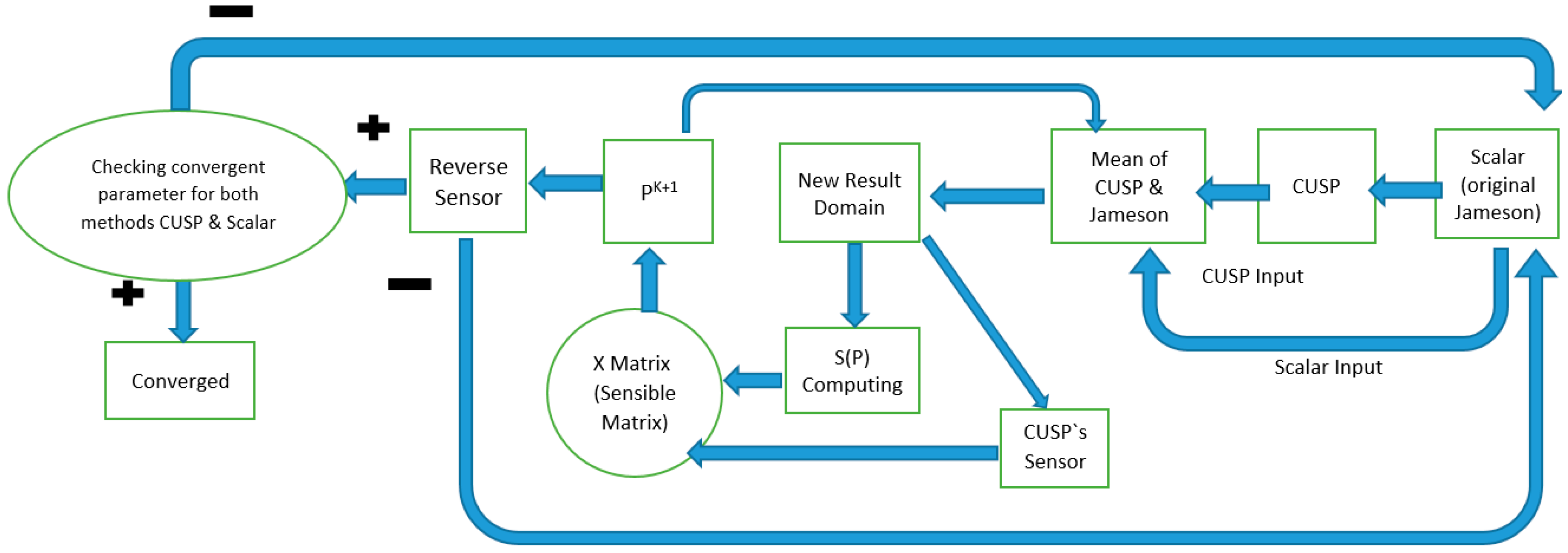
Figure 3.
Stage algorithm of hybrid finite volume method (scalar (original Jameson) + CUSP) for modeling the two-phase nucleating flow in Laval nozzle, mid and tip-section blades of a steam turbine with using the optimized convergence parameter ().
Figure 3.
Stage algorithm of hybrid finite volume method (scalar (original Jameson) + CUSP) for modeling the two-phase nucleating flow in Laval nozzle, mid and tip-section blades of a steam turbine with using the optimized convergence parameter ().
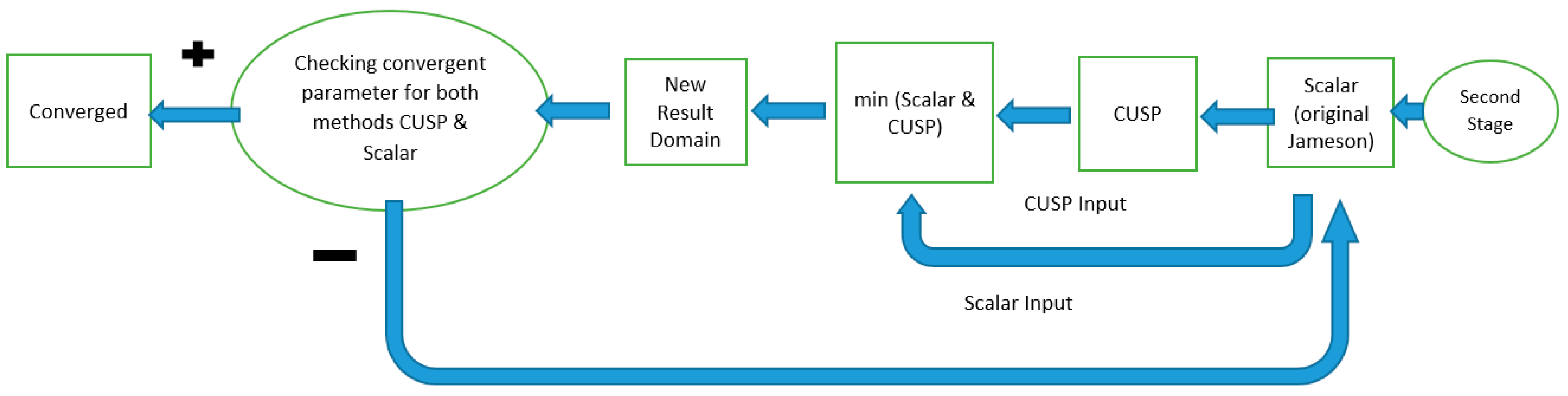
Figure 4.
Grid computing standard for Moore nozzle type A [40].
Figure 4.
Grid computing standard for Moore nozzle type A [40].

Figure 5.
Comparing the distribution of static pressure with inlet stagnation pressure on the center line stream (MP) along the nozzle results of the scalar and hybrid (scalar + CUSP + inverse) numerical methods and comparing with experimental data in supersonic outlet flow for Moore nozzle type A [40].

Figure 6.
Distribution variation of logarithmic radius along the nozzle in central line stream (MP) results of scalar and hybrid (scalar + CUSP + inverse) numerical methods and comparing with the experimental droplet radius in supersonic outlet flow for Moore nozzle type A [40].
Figure 6.
Distribution variation of logarithmic radius along the nozzle in central line stream (MP) results of scalar and hybrid (scalar + CUSP + inverse) numerical methods and comparing with the experimental droplet radius in supersonic outlet flow for Moore nozzle type A [40].
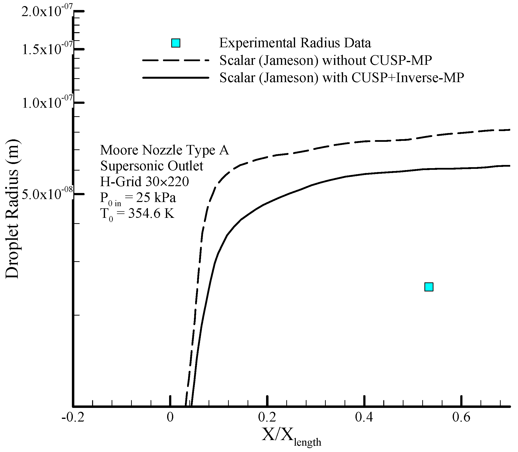
Figure 7.
Grid computing standard for Moore nozzle type B [40].
Figure 7.
Grid computing standard for Moore nozzle type B [40].
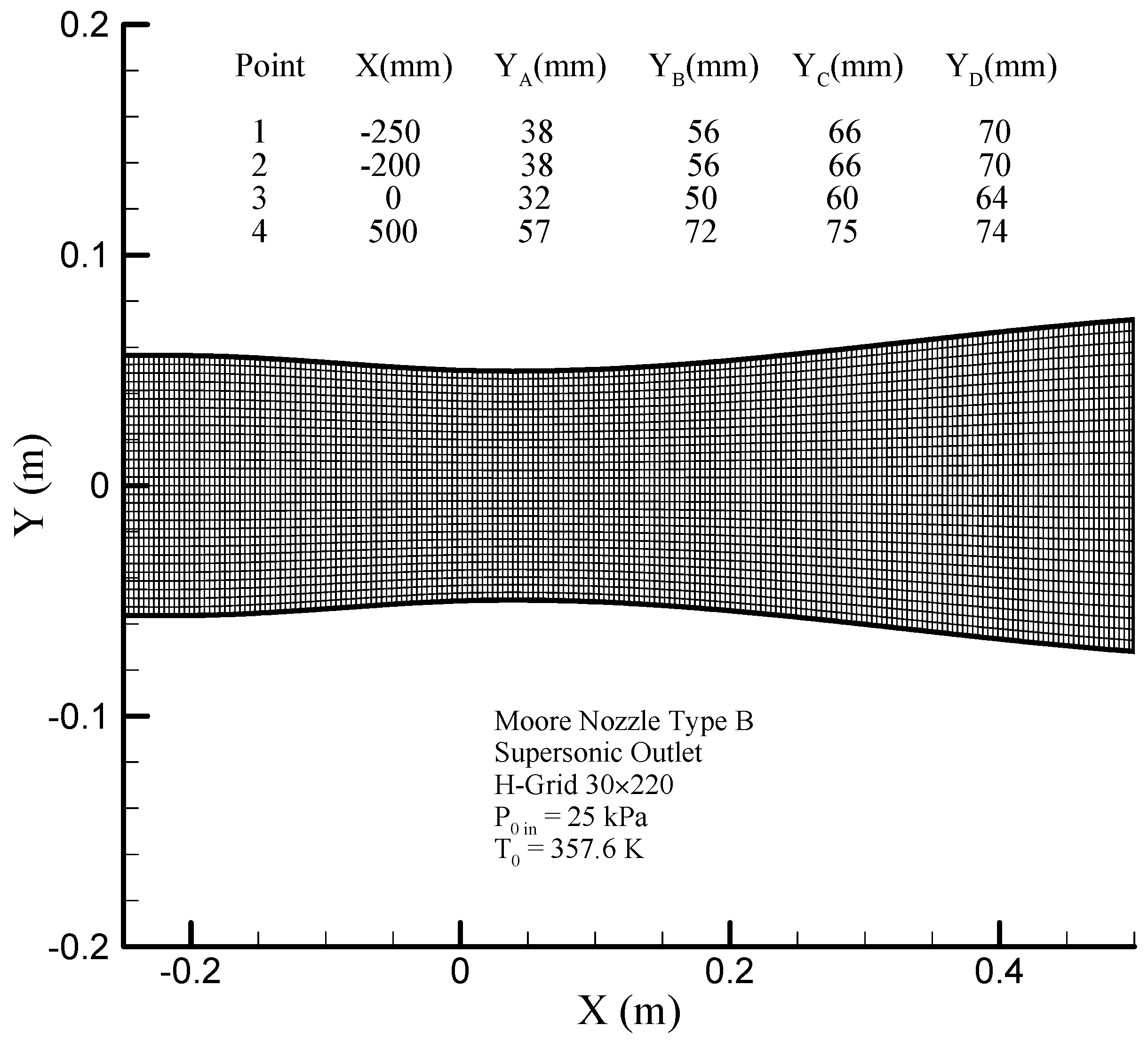
Figure 8.
Comparing the distribution of static pressure with inlet stagnation pressure on the center line stream (MP) along the nozzles results of the scalar and hybrid (scalar + CUSP + inverse) numerical methods and comparing with experimental data in supersonic outlet flow for Moore nozzle type B [40].

Figure 9.
Comparing distribution variation of logarithmic radius along the nozzle in central line stream (MP) results of scalar and hybrid (scalar + CUSP+ inverse) numerical methods and comparing with the experimental radius in supersonic outlet flow for Moore nozzle type B [40].
Figure 9.
Comparing distribution variation of logarithmic radius along the nozzle in central line stream (MP) results of scalar and hybrid (scalar + CUSP+ inverse) numerical methods and comparing with the experimental radius in supersonic outlet flow for Moore nozzle type B [40].

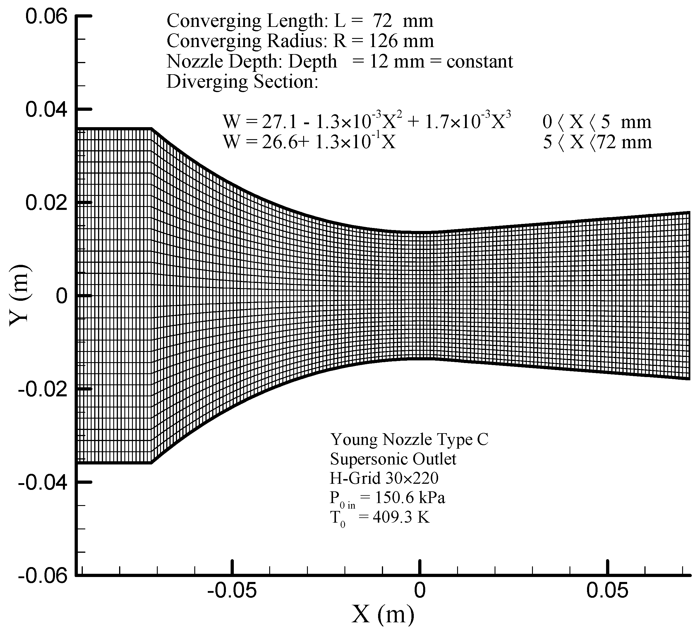
Figure 11.
Comparing the distribution of static pressure with inlet stagnation pressure on the center line stream (MP) along the nozzles results of the scalar and hybrid (scalar + CUSP + inverse) numerical methods and comparing with experimental data in supersonic outlet flow for Young nozzle type C [43].


Figure 13.
Comparing the distribution of static pressure with inlet stagnation pressure on the center line stream along the nozzles results of the scalar and hybrid (scalar + CUSP + inverse) numerical methods and comparing with experimental data in supersonic outlet flow for Barschdorff nozzle [44].
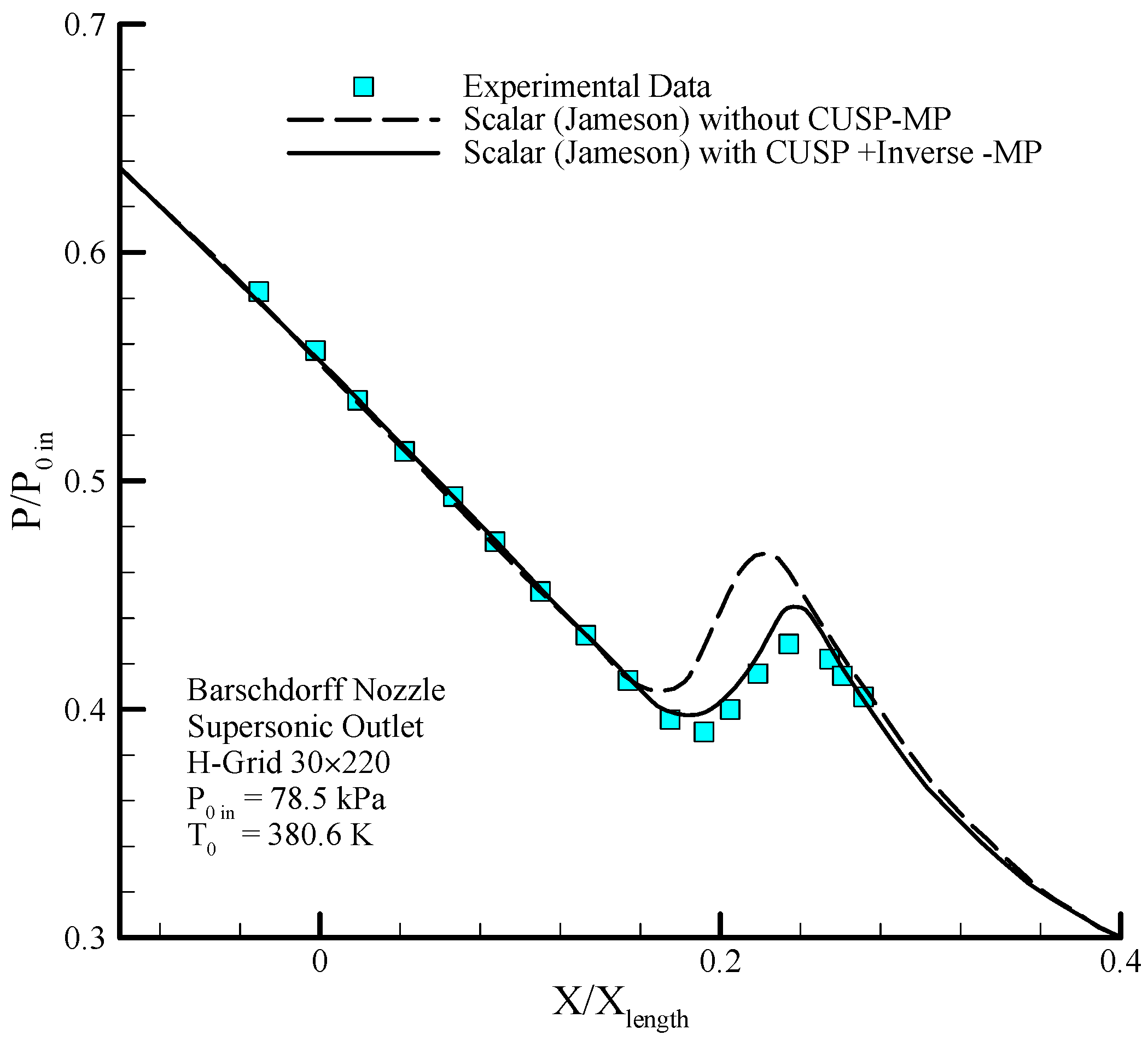
Figure 14.
Distribution variation of logarithmic radius along the nozzle in central line stream (MP) results of scalar and hybrid (scalar + CUSP + inverse) numerical methods and comparing with the experimental radius in supersonic outlet flow for Barschdorff nozzle [44].
Figure 14.
Distribution variation of logarithmic radius along the nozzle in central line stream (MP) results of scalar and hybrid (scalar + CUSP + inverse) numerical methods and comparing with the experimental radius in supersonic outlet flow for Barschdorff nozzle [44].
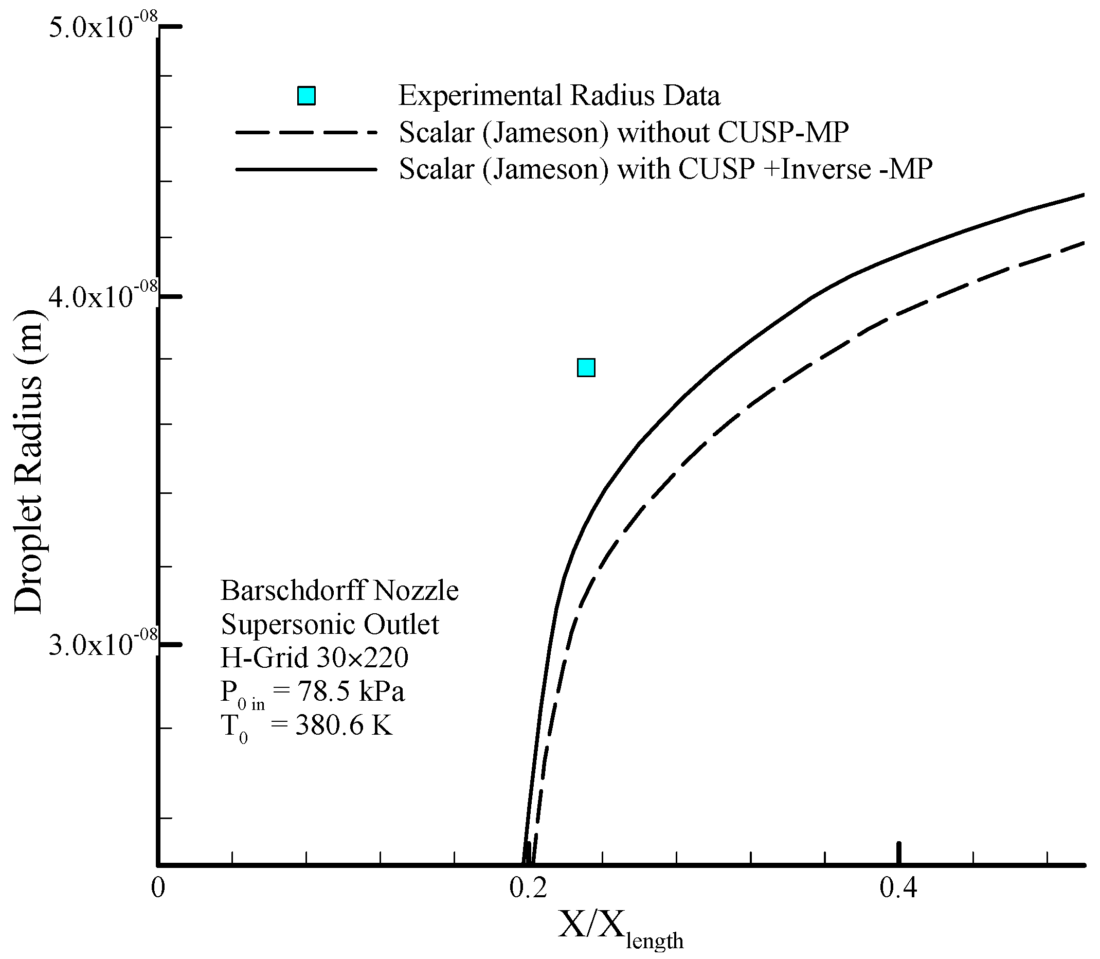

Figure 16.
Comparing the distribution of static pressure with inlet stagnation pressure along the blades on suction side (SS) results of the scalar and hybrid (scalar + CUSP + inverse) numerical methods and comparing with experimental data in supersonic outlet flow for dry steam in mid-section turbine blade [1,12].
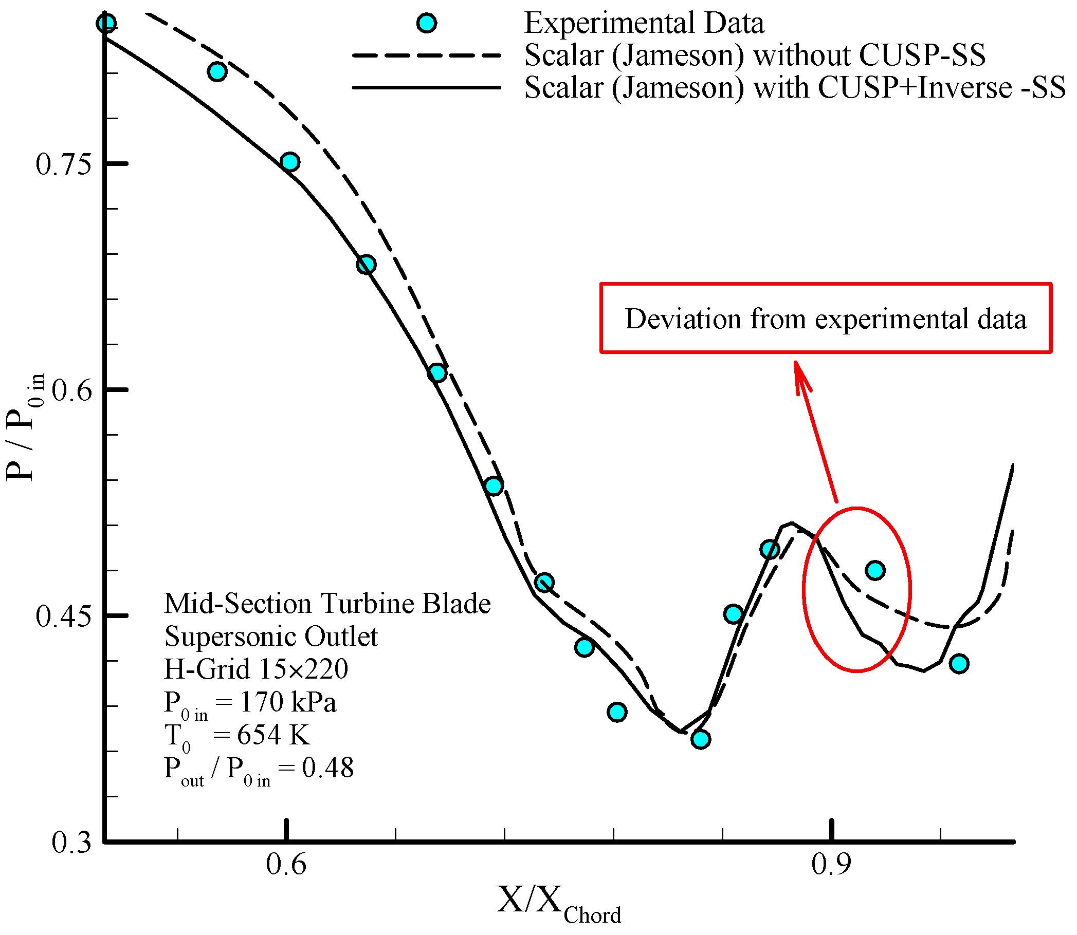
Figure 17.
The impact value of convergence parameter values improvement on the change of mass flow percent with inverse method.
Figure 17.
The impact value of convergence parameter values improvement on the change of mass flow percent with inverse method.
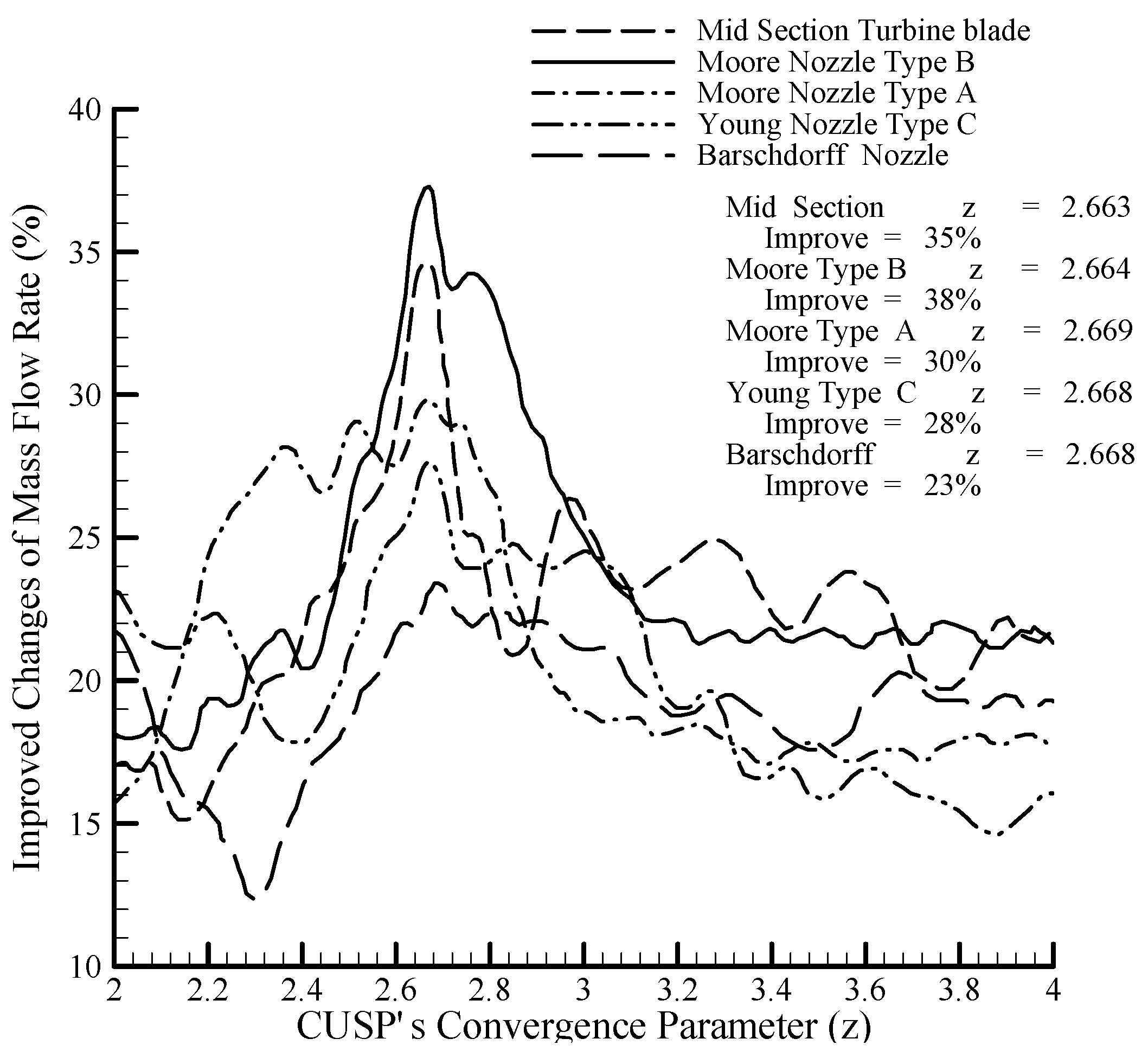
Figure 18.
The percent of CUSP method in hybrid method (scalar + CUSP) for flow modeling between mid-section turbine blade use of inverse method.
Figure 18.
The percent of CUSP method in hybrid method (scalar + CUSP) for flow modeling between mid-section turbine blade use of inverse method.


Figure 20.
Comparing the distribution of static pressure with inlet stagnation pressure on the center line stream (MP) along the nozzle results of the scalar and hybrid (scalar + CUSP, ) numerical methods and comparing with experimental data for supersonic outlet flow in Young nozzle type L [10,43]. Note: The Laval nozzle is adiabatic, only the convergent duct is reversible.
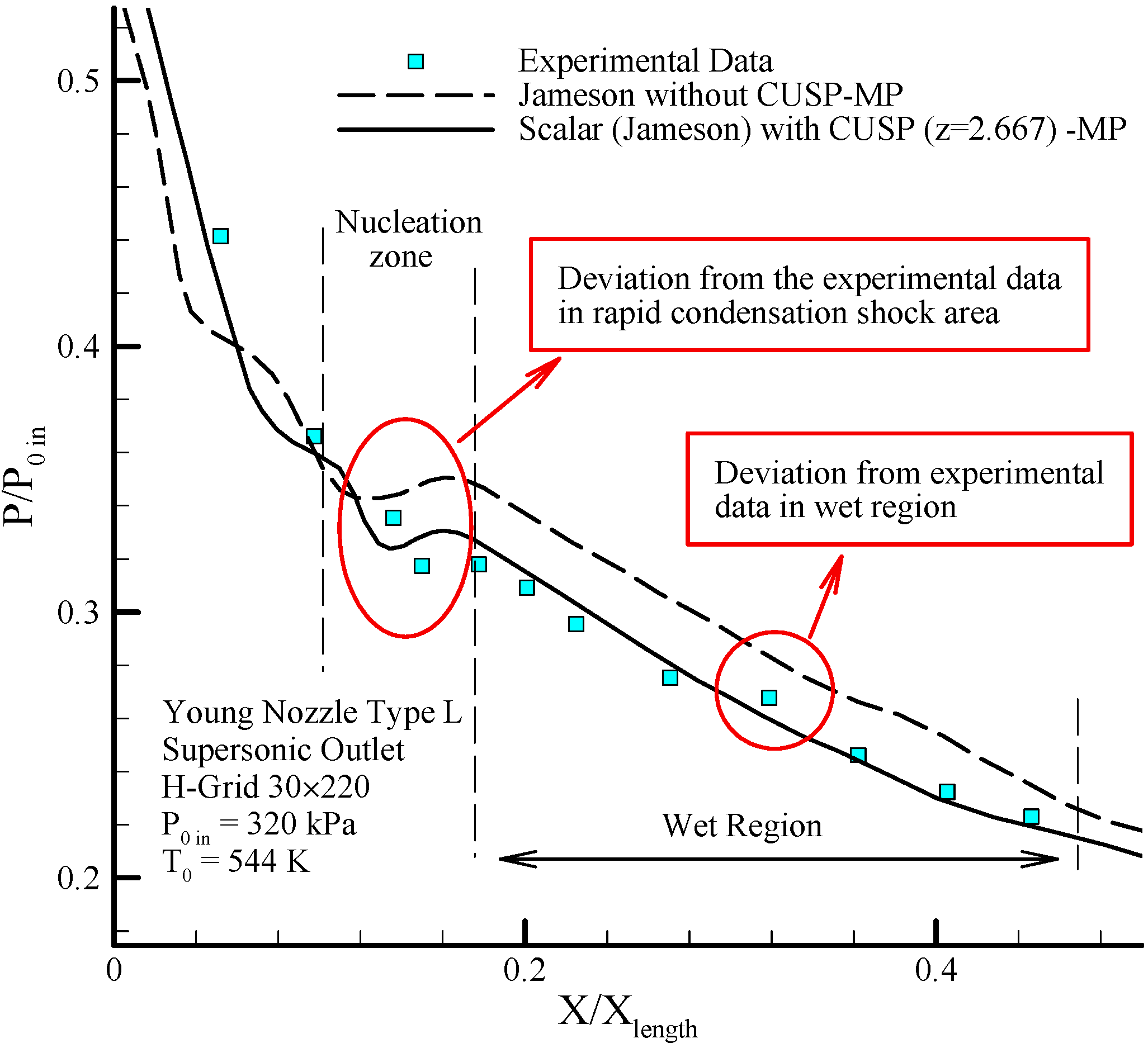
Figure 21.
Comparing the distribution percent variation of stagnation pressure with inlet stagnation pressure on the center line stream (MP) along the nozzles results of the Scalar and hybrid (Scalar + CUSP, ) numerical methods for supersonic outlet flow in Young nozzle type L.
Figure 21.
Comparing the distribution percent variation of stagnation pressure with inlet stagnation pressure on the center line stream (MP) along the nozzles results of the Scalar and hybrid (Scalar + CUSP, ) numerical methods for supersonic outlet flow in Young nozzle type L.
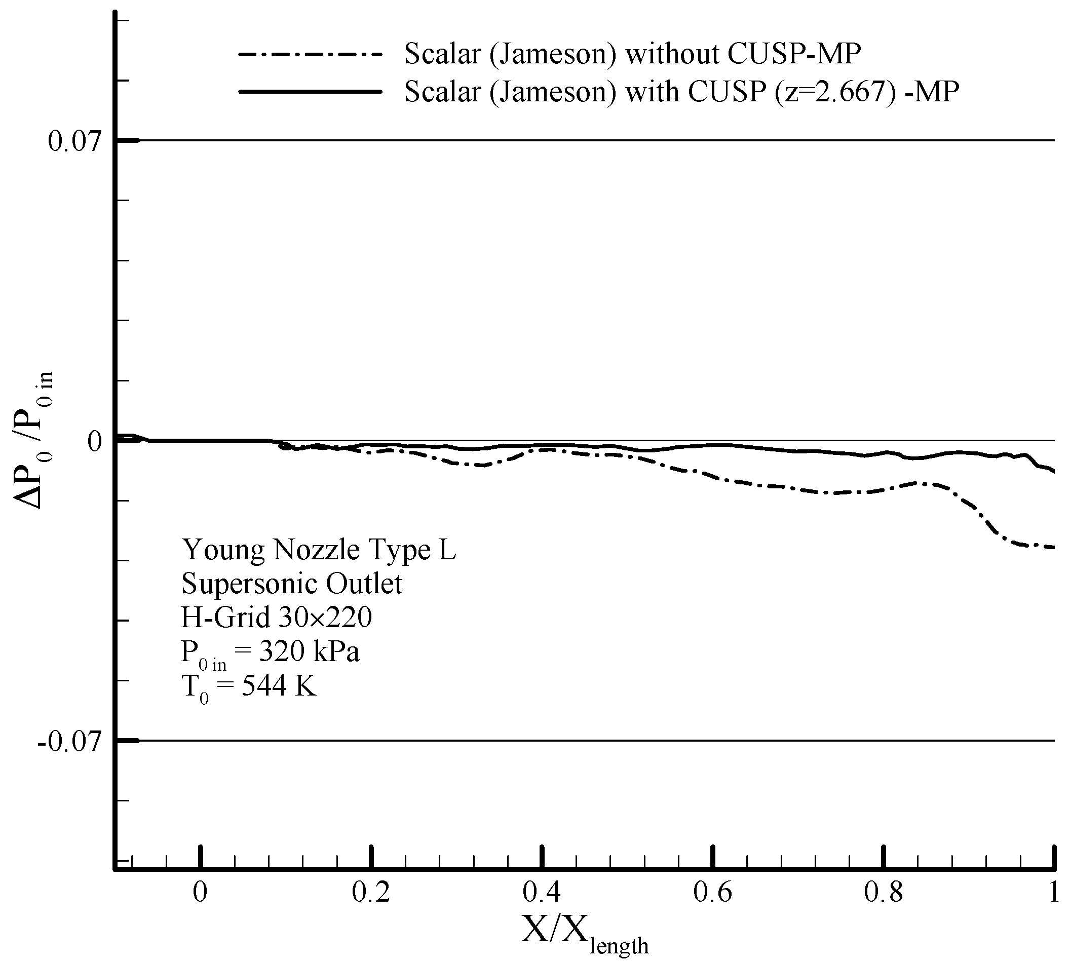
Figure 22.
Distribution variation of wetness fraction on the center line stream (MP) along the nozzles results of the scalar and hybrid (scalar + CUSP, ) numerical methods for supersonic outlet flow in Young nozzle type L.
Figure 22.
Distribution variation of wetness fraction on the center line stream (MP) along the nozzles results of the scalar and hybrid (scalar + CUSP, ) numerical methods for supersonic outlet flow in Young nozzle type L.
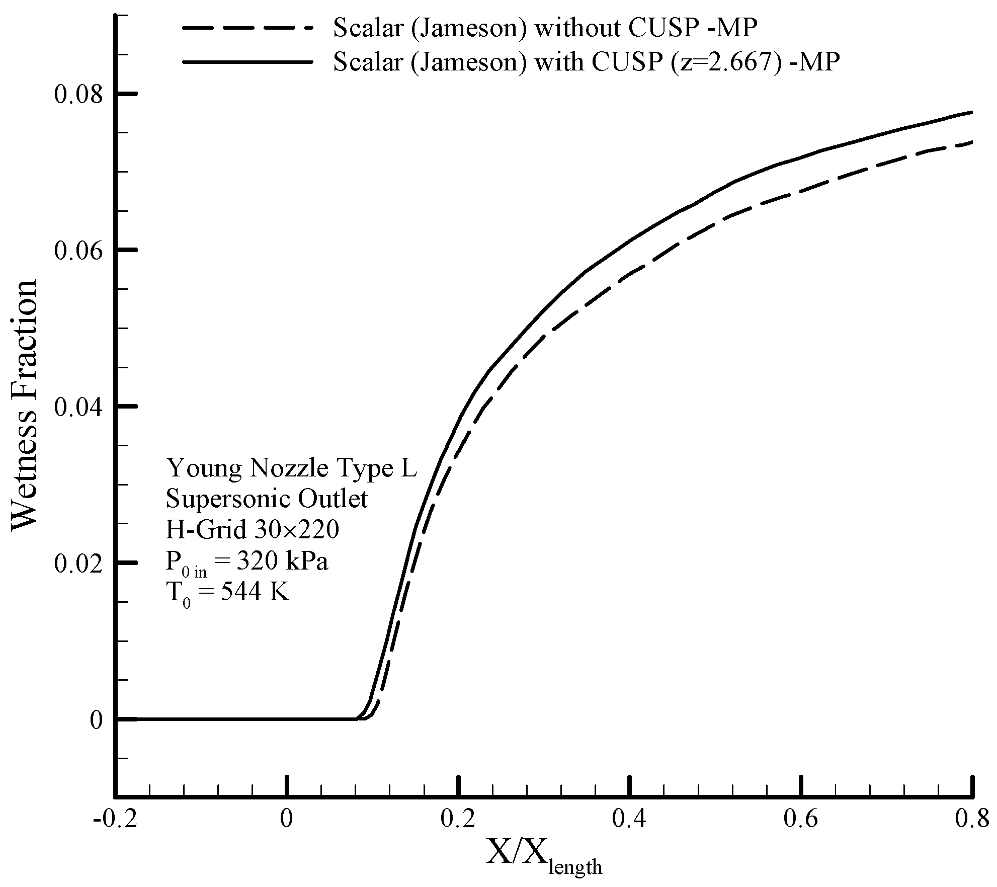
Figure 23.
Distribution variation of nucleation rate on the center line stream (MP) along the nozzles results of the scalar and hybrid (scalar + CUSP, ) numerical methods for supersonic outlet flow in Young nozzle type L.
Figure 23.
Distribution variation of nucleation rate on the center line stream (MP) along the nozzles results of the scalar and hybrid (scalar + CUSP, ) numerical methods for supersonic outlet flow in Young nozzle type L.

Figure 24.
Distribution variation of logarithmic radius drops along the nozzle in central line stream (MP) results of scalar and hybrid (scalar + CUSP, ) numerical methods and comparing with experimental data for supersonic outlet flow in Young nozzle type L [10,43].
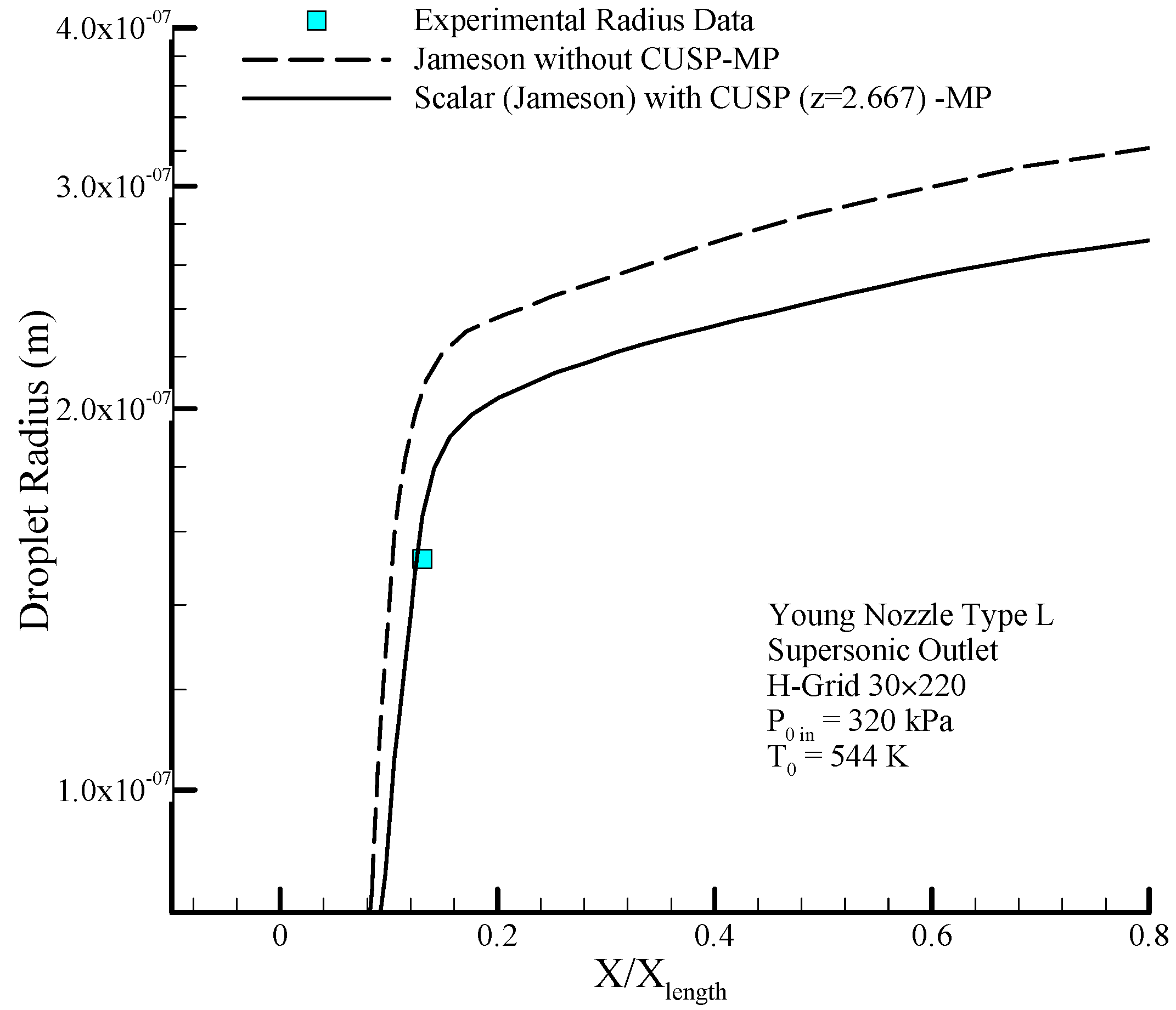
Figure 25.
Distribution variation percent of mass flow on the center line stream (MP) along the nozzles results of the Scalar and hybrid (Scalar + CUSP, ) numerical methods for supersonic outlet flow in Young nozzle type L.
Figure 25.
Distribution variation percent of mass flow on the center line stream (MP) along the nozzles results of the Scalar and hybrid (Scalar + CUSP, ) numerical methods for supersonic outlet flow in Young nozzle type L.
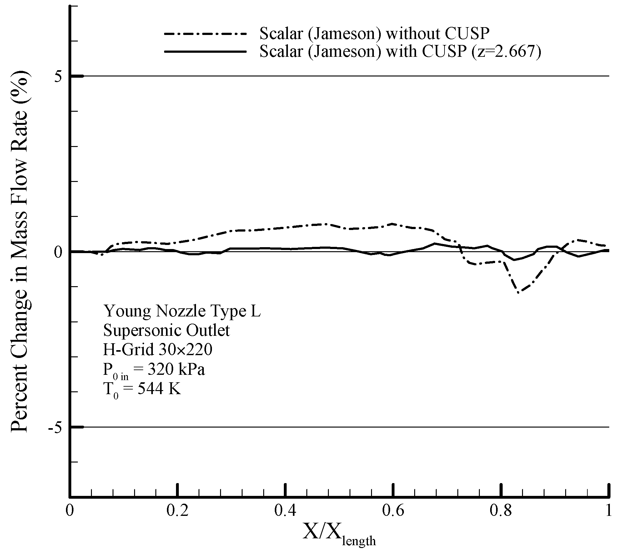
Figure 26.
Distribution of static pressure with inlet stagnation pressure along the blades on the suction side and the pressure results of numerical hybrid (scalar + CUSP, ) method and comparing with experimental data for supersonic outlet flow in mid-section blade [12].
Figure 26.
Distribution of static pressure with inlet stagnation pressure along the blades on the suction side and the pressure results of numerical hybrid (scalar + CUSP, ) method and comparing with experimental data for supersonic outlet flow in mid-section blade [12].
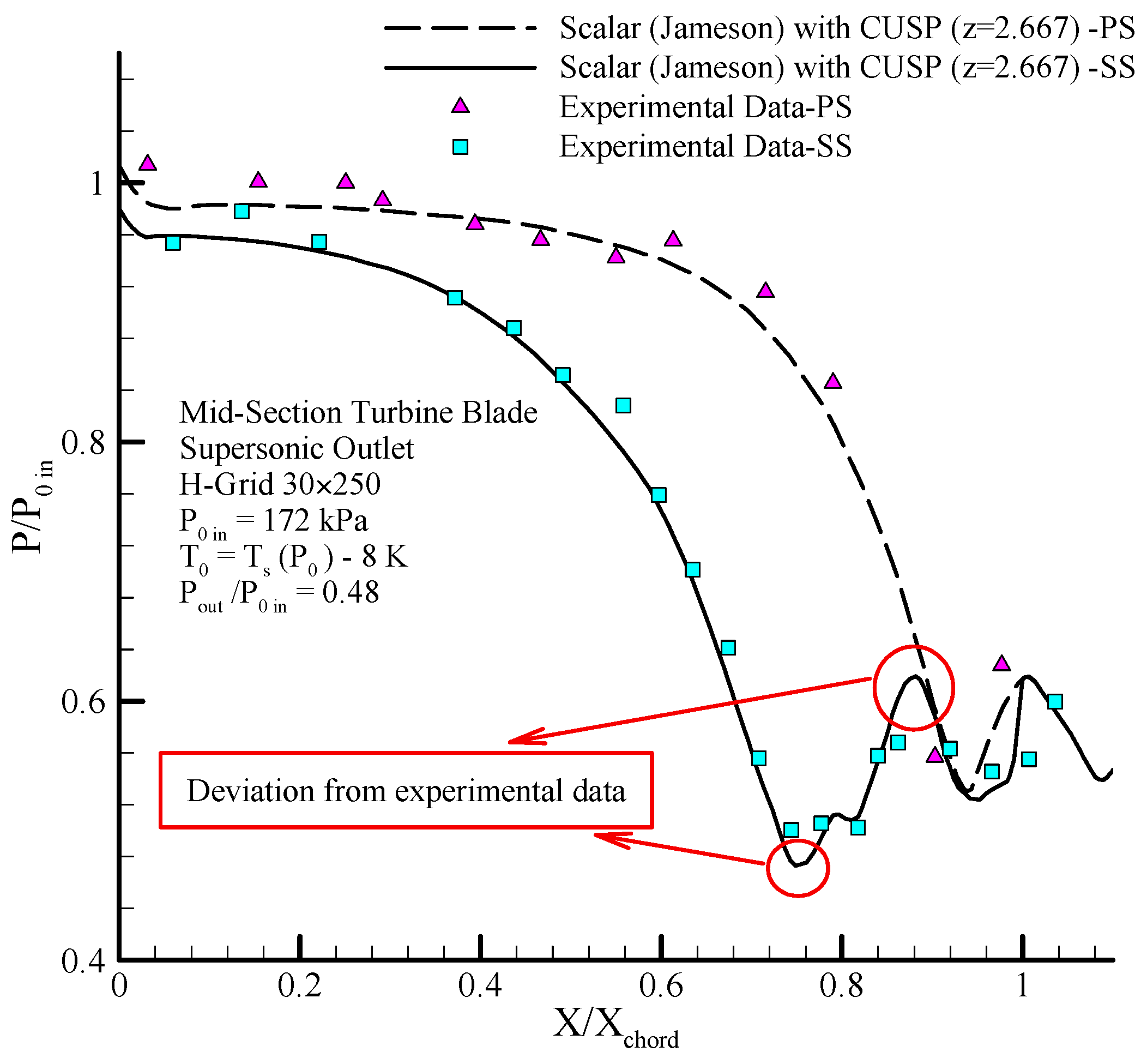
Figure 27.
Distribution of static pressure with inlet stagnation pressure along the blades on suction side results of the scalar and hybrid (scalar + CUSP + ) numerical methods and comparing with experimental data for supersonic outlet flow in mid-section blade [12].
Figure 27.
Distribution of static pressure with inlet stagnation pressure along the blades on suction side results of the scalar and hybrid (scalar + CUSP + ) numerical methods and comparing with experimental data for supersonic outlet flow in mid-section blade [12].

Figure 28.
Comparing the distribution percent variation of stagnation pressure with inlet stagnation pressure along blade in central line stream (MP) results of the scalar and hybrid (scalar + CUSP, ) numerical methods for supersonic outlet flow in mid-section blade.
Figure 28.
Comparing the distribution percent variation of stagnation pressure with inlet stagnation pressure along blade in central line stream (MP) results of the scalar and hybrid (scalar + CUSP, ) numerical methods for supersonic outlet flow in mid-section blade.

Figure 29.
Distribution variation of wetness fraction along the suction side results of the scalar and hybrid (scalar + CUSP, ) numerical methods for supersonic outlet flow in mid-section blade.
Figure 29.
Distribution variation of wetness fraction along the suction side results of the scalar and hybrid (scalar + CUSP, ) numerical methods for supersonic outlet flow in mid-section blade.
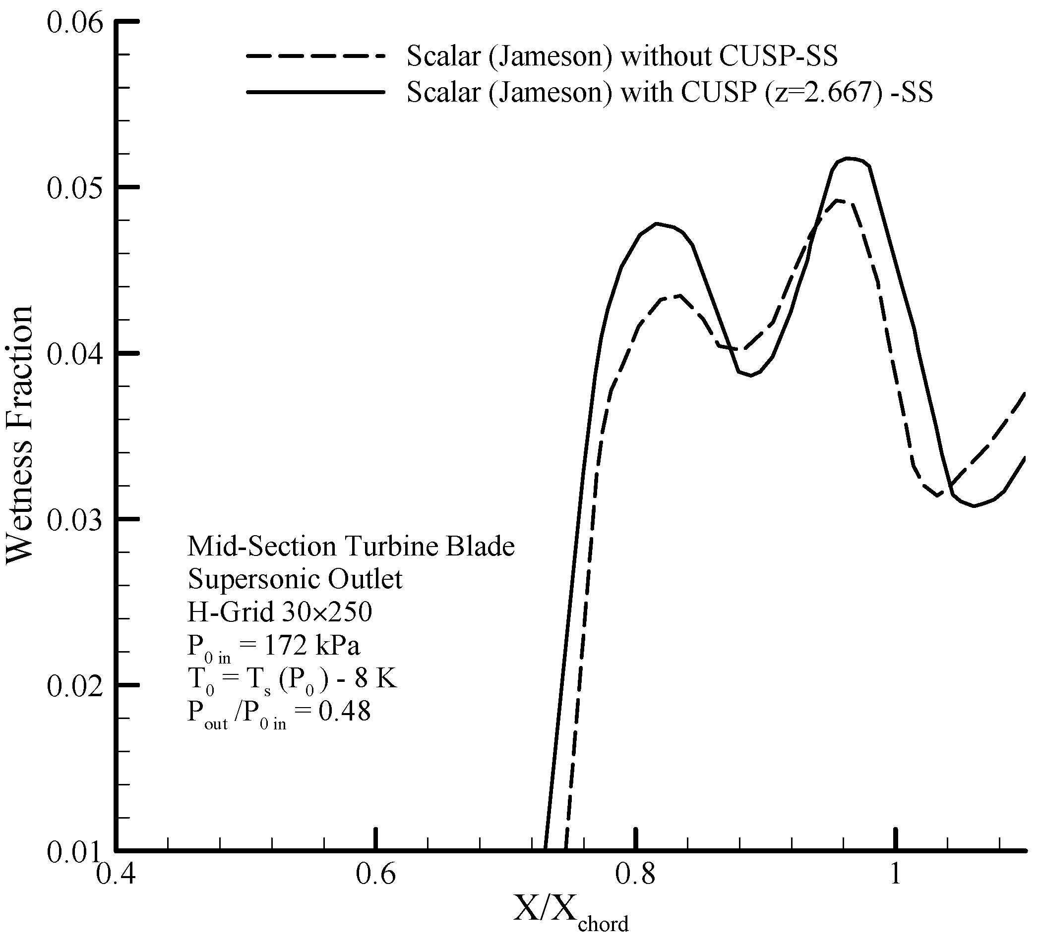
Figure 30.
Distribution variation of nucleation rate on suction side results of the scalar and hybrid (scalar + CUSP, ) numerical methods for supersonic outlet flow in mid-section blade.
Figure 30.
Distribution variation of nucleation rate on suction side results of the scalar and hybrid (scalar + CUSP, ) numerical methods for supersonic outlet flow in mid-section blade.
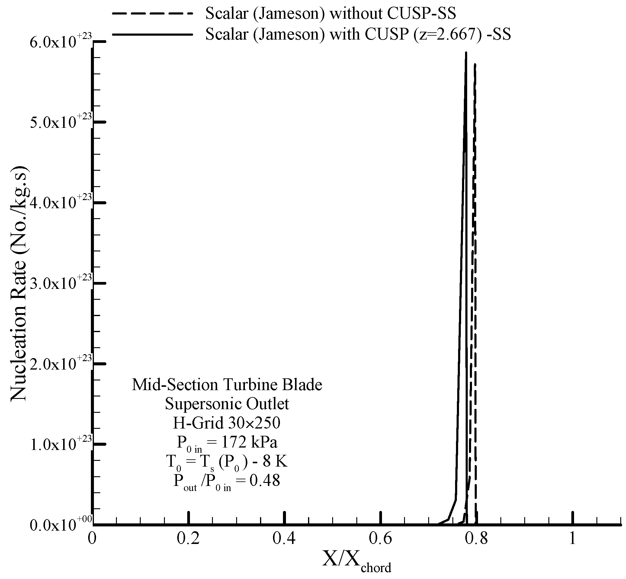
Figure 31.
Distribution variation of logarithmic radius droplets along the suction sides and pressure stream results of the scalar and hybrid (scalar + CUSP, ) numerical methods and comparing with experimental data for supersonic outlet flow in mid-section blade [12].
Figure 31.
Distribution variation of logarithmic radius droplets along the suction sides and pressure stream results of the scalar and hybrid (scalar + CUSP, ) numerical methods and comparing with experimental data for supersonic outlet flow in mid-section blade [12].

Figure 32.
Distribution variation percent of mass flow results of the scalar and hybrid (scalar + CUSP, ) numerical methods for supersonic outlet flow in mid-section blade.
Figure 32.
Distribution variation percent of mass flow results of the scalar and hybrid (scalar + CUSP, ) numerical methods for supersonic outlet flow in mid-section blade.
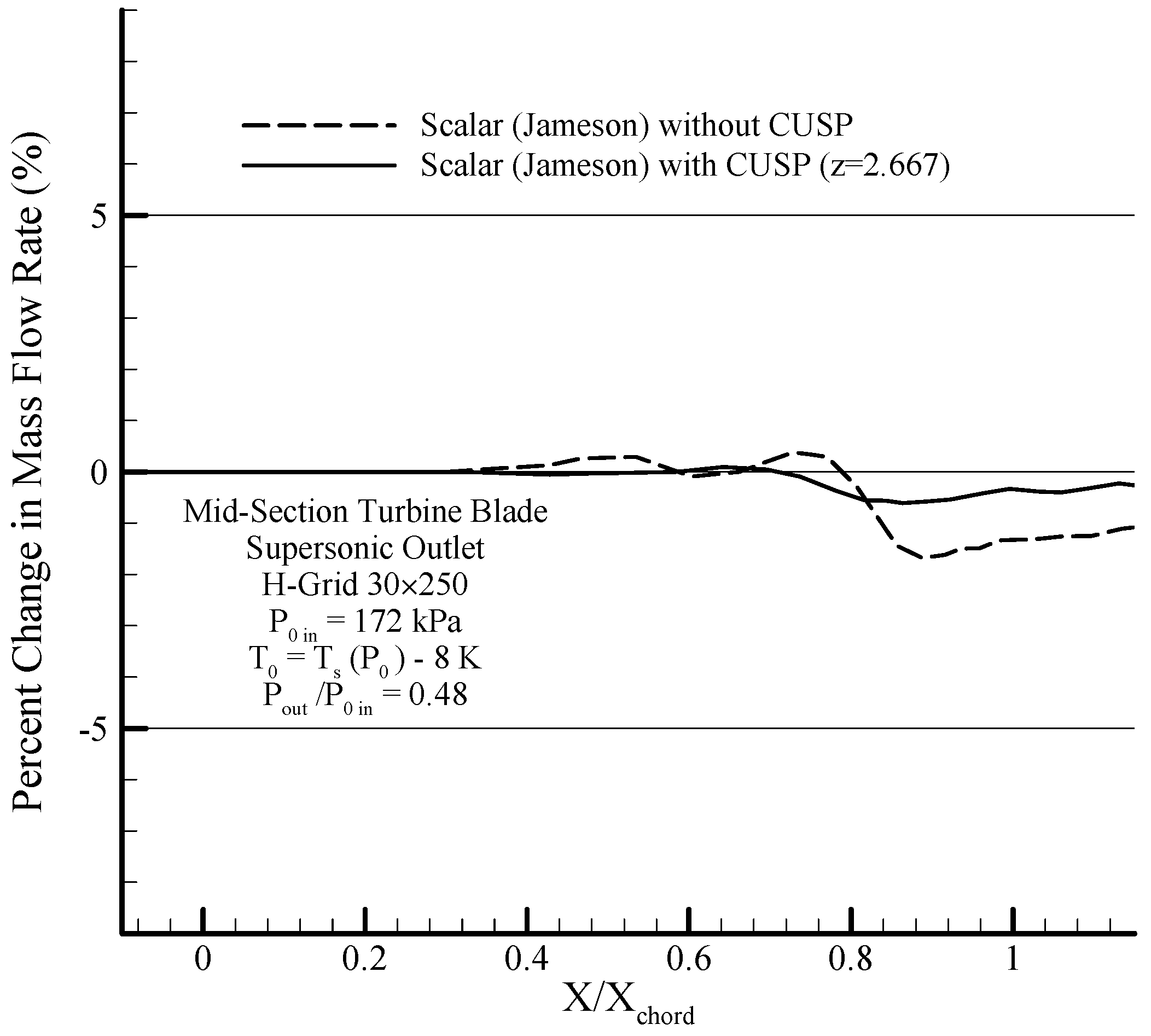
Figure 33.
Distribution variation of logarithmic residual of density results for the hybrid (Scalar + CUSP, ) method (a) for supersonic outlet flow in mid-section blade; (b) with 100 additional iterations after convergence for supersonic outlet flow in mid-section blade.
Figure 33.
Distribution variation of logarithmic residual of density results for the hybrid (Scalar + CUSP, ) method (a) for supersonic outlet flow in mid-section blade; (b) with 100 additional iterations after convergence for supersonic outlet flow in mid-section blade.


Figure 35.
Distribution of static pressure with inlet stagnation pressure along the blades on the suction pressure side and central line stream results of the hybrid (Scalar + CUSP, ) numerical method and comparing with experimental data for supersonic outlet flow in tip-section blade [45].
Figure 35.
Distribution of static pressure with inlet stagnation pressure along the blades on the suction pressure side and central line stream results of the hybrid (Scalar + CUSP, ) numerical method and comparing with experimental data for supersonic outlet flow in tip-section blade [45].
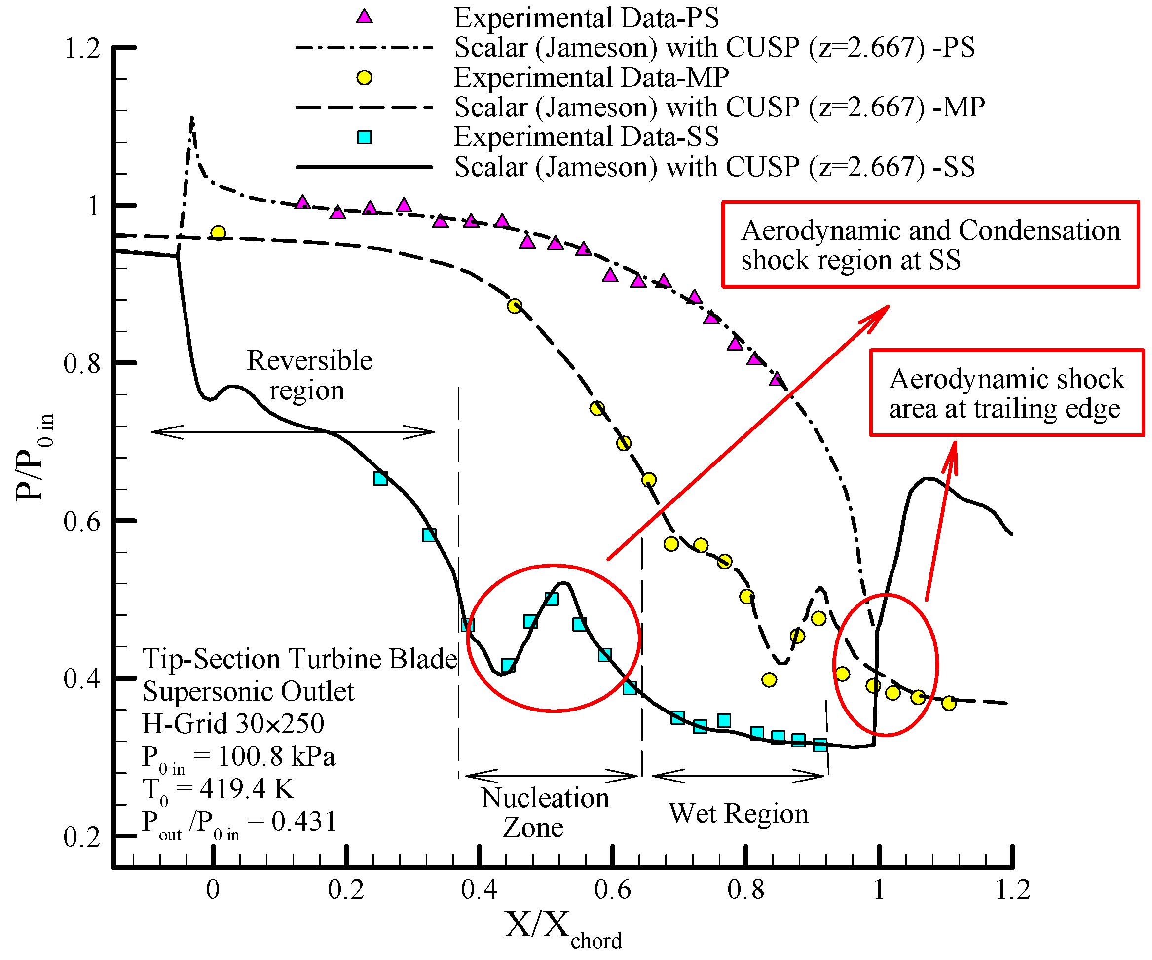
Figure 36.
Comparing distribution of static pressure with inlet stagnation pressure along the blades in central line (MP) results of the scalar and hybrid (scalar + CUSP, ) numerical methods and comparing with experimental data for supersonic outlet flow in tip-section blade [45].
Figure 36.
Comparing distribution of static pressure with inlet stagnation pressure along the blades in central line (MP) results of the scalar and hybrid (scalar + CUSP, ) numerical methods and comparing with experimental data for supersonic outlet flow in tip-section blade [45].
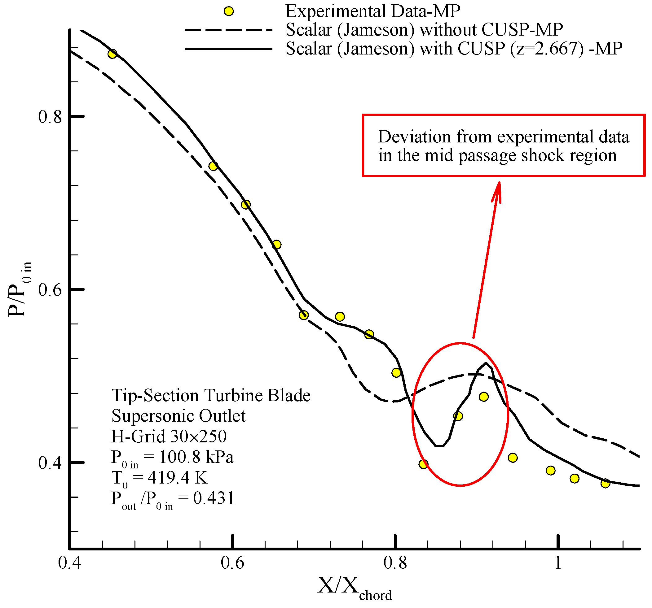
Figure 37.
Comparing the distribution percent variation of stagnation pressure with inlet stagnation pressure along blade in central line stream (MP) results of the scalar and hybrid (scalar + CUSP, ) numerical methods for supersonic outlet flow in tip-section blade.
Figure 37.
Comparing the distribution percent variation of stagnation pressure with inlet stagnation pressure along blade in central line stream (MP) results of the scalar and hybrid (scalar + CUSP, ) numerical methods for supersonic outlet flow in tip-section blade.

Figure 38.
Results of the numerical hybrid (scalar + CUSP, ) method between blades for supersonic outlet flow in tip-section blade (a) Contours of Mach; (b) Contours of wetness fraction.
Figure 38.
Results of the numerical hybrid (scalar + CUSP, ) method between blades for supersonic outlet flow in tip-section blade (a) Contours of Mach; (b) Contours of wetness fraction.
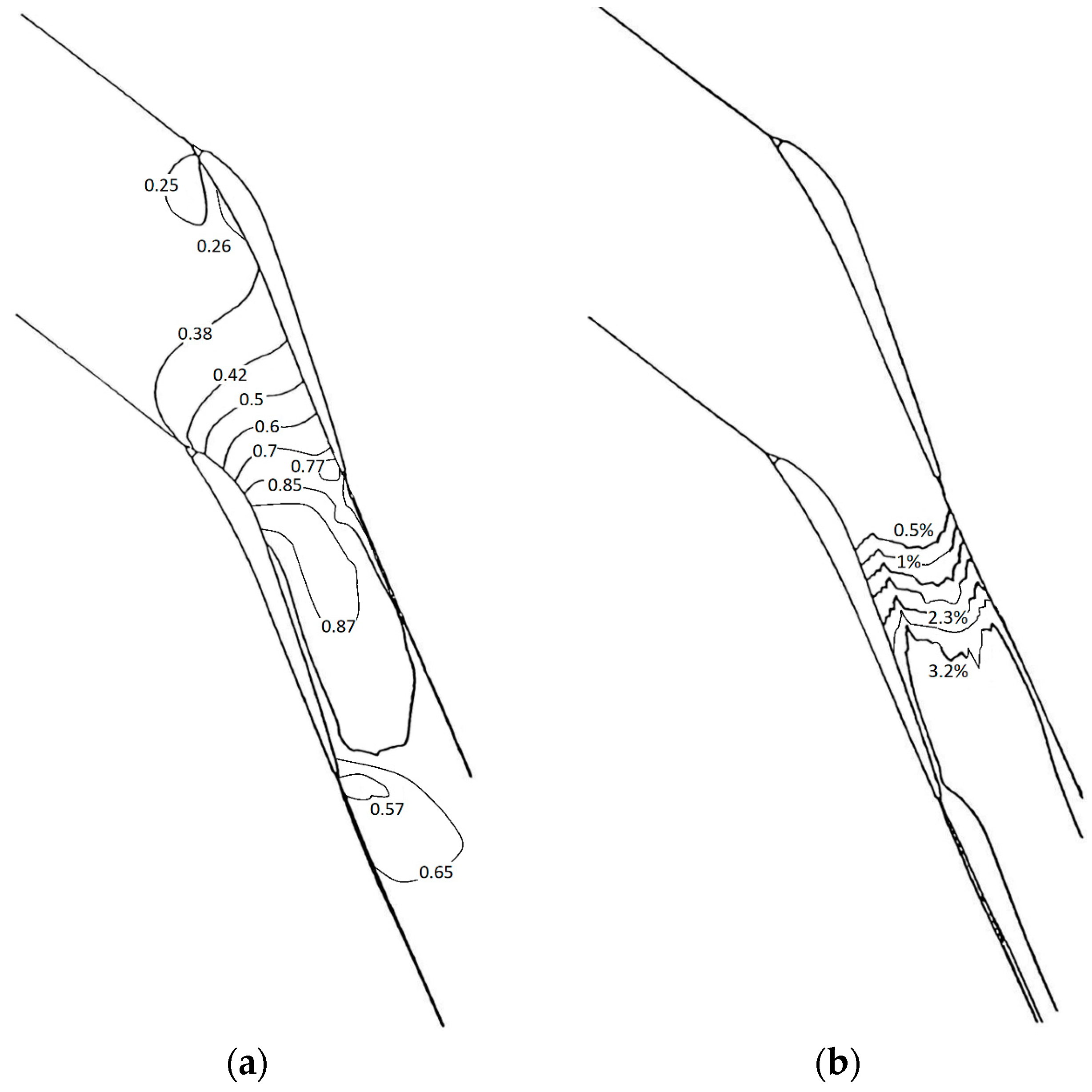
Figure 39.
Distribution variation of wetness fraction along the suction side (SS) and central stream (MP) results of the scalar and hybrid (scalar + CUSP, ) numerical methods for supersonic outlet flow in tip-section blade.
Figure 39.
Distribution variation of wetness fraction along the suction side (SS) and central stream (MP) results of the scalar and hybrid (scalar + CUSP, ) numerical methods for supersonic outlet flow in tip-section blade.
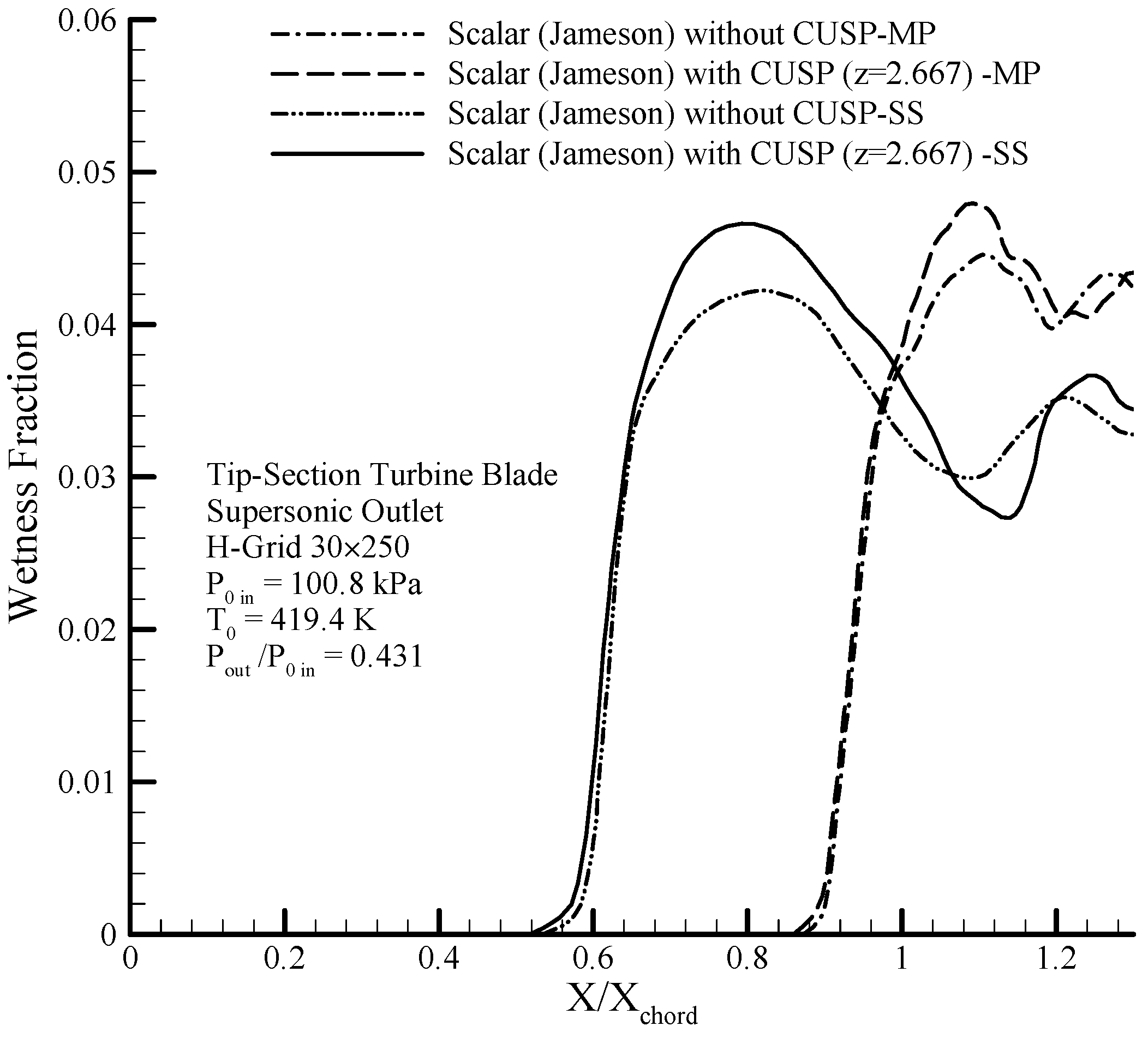
Figure 40.
Distribution variation of nucleation rate on suction side results of the scalar and hybrid (scalar + CUSP, ) numerical methods for supersonic outlet flow in tip-section blade.
Figure 40.
Distribution variation of nucleation rate on suction side results of the scalar and hybrid (scalar + CUSP, ) numerical methods for supersonic outlet flow in tip-section blade.
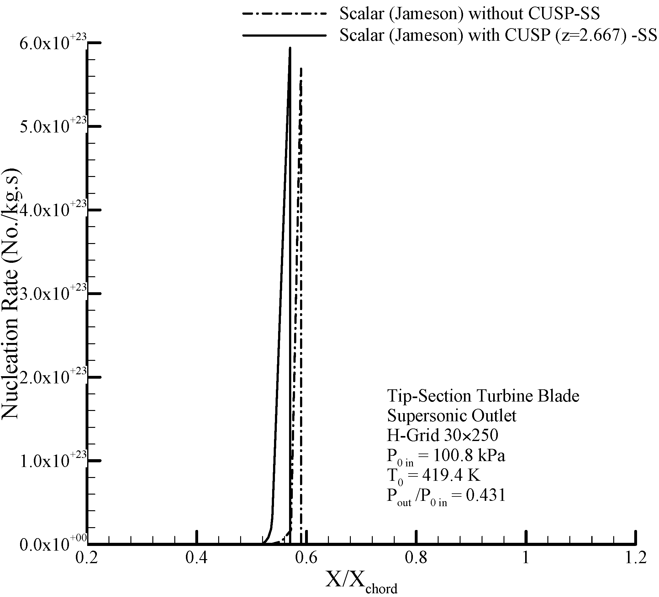
Figure 41.
Distribution variation of logarithmic radius drops along the suction sides and central stream results of the scalar and hybrid (scalar + CUSP, ) numerical methods and comparing with experimental data in supersonic outlet flow on tip-section blade [45].
Figure 41.
Distribution variation of logarithmic radius drops along the suction sides and central stream results of the scalar and hybrid (scalar + CUSP, ) numerical methods and comparing with experimental data in supersonic outlet flow on tip-section blade [45].
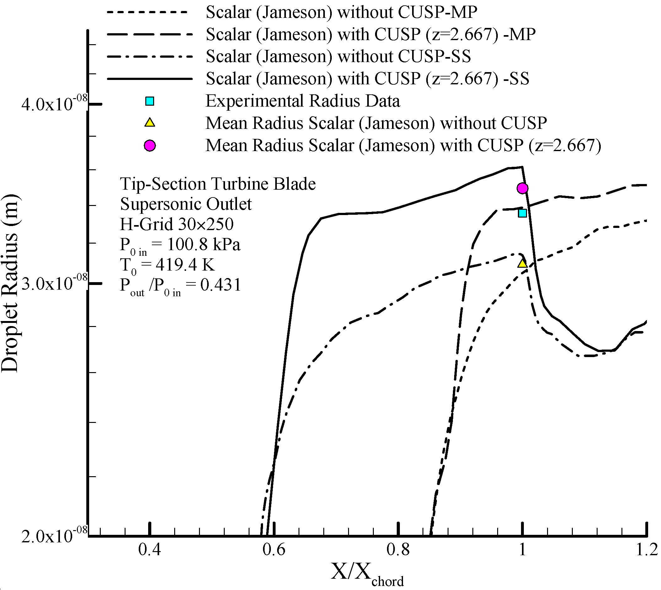
Figure 42.
Distribution variation percent of mass flow results of the scalar and hybrid (scalar + CUSP, ) numerical methods for supersonic outlet flow in tip-section blade.
Figure 42.
Distribution variation percent of mass flow results of the scalar and hybrid (scalar + CUSP, ) numerical methods for supersonic outlet flow in tip-section blade.
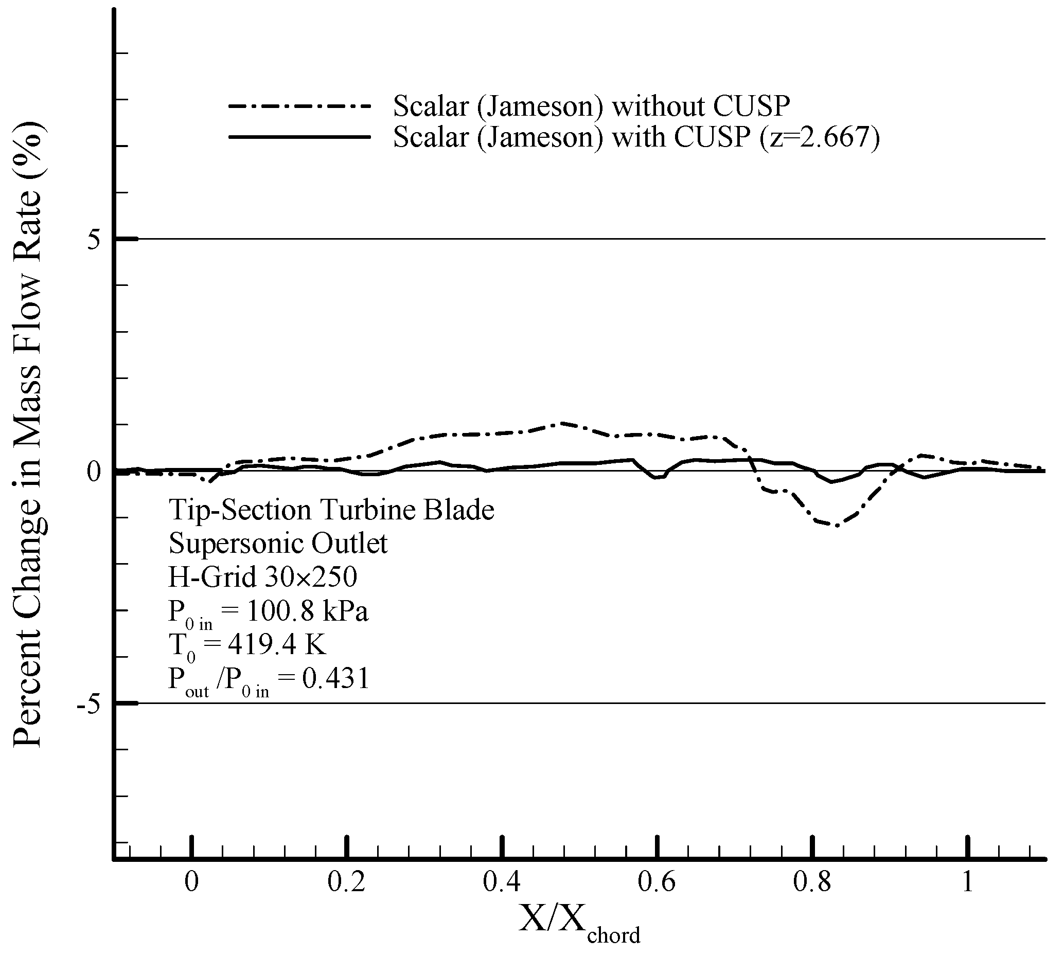

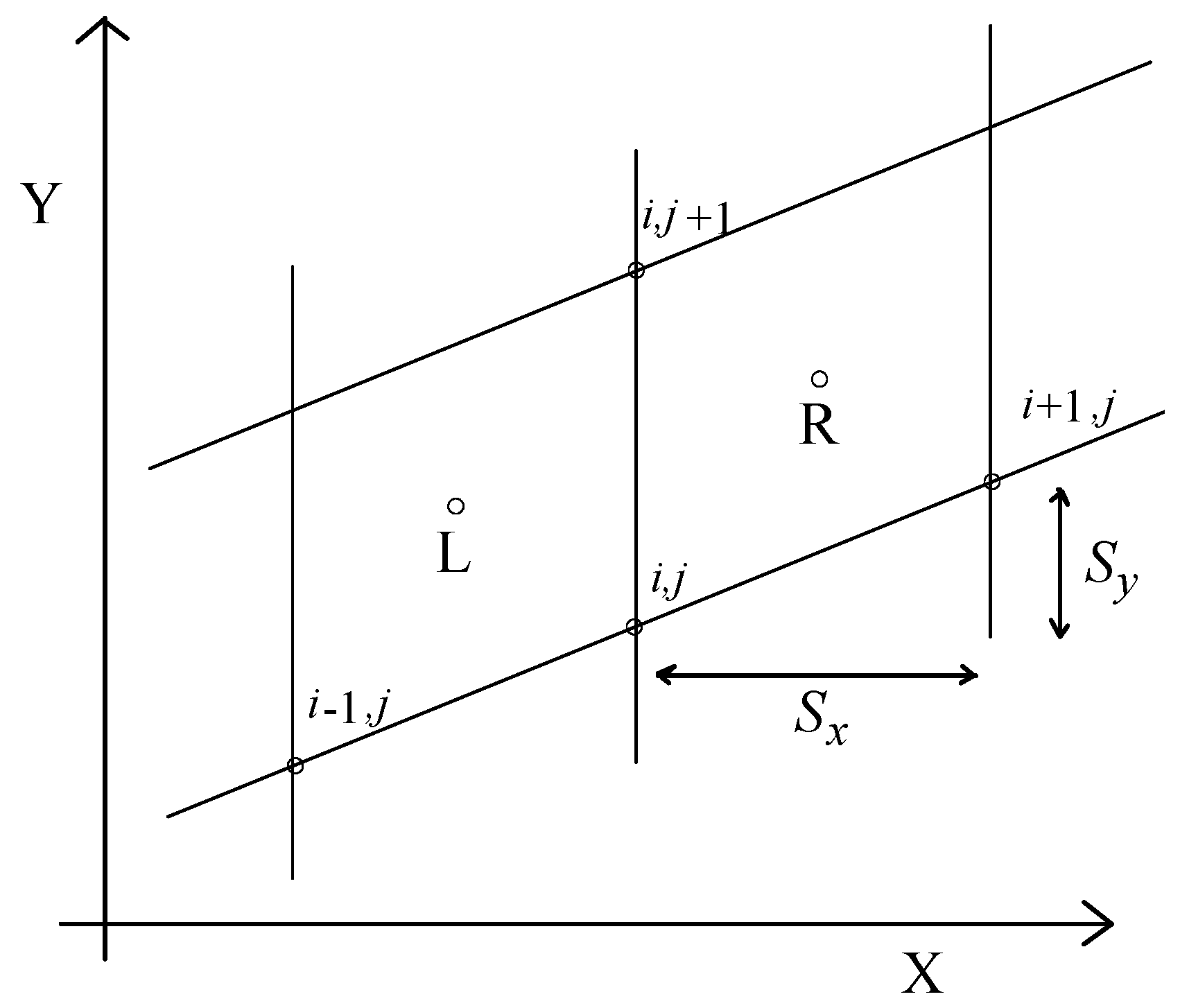
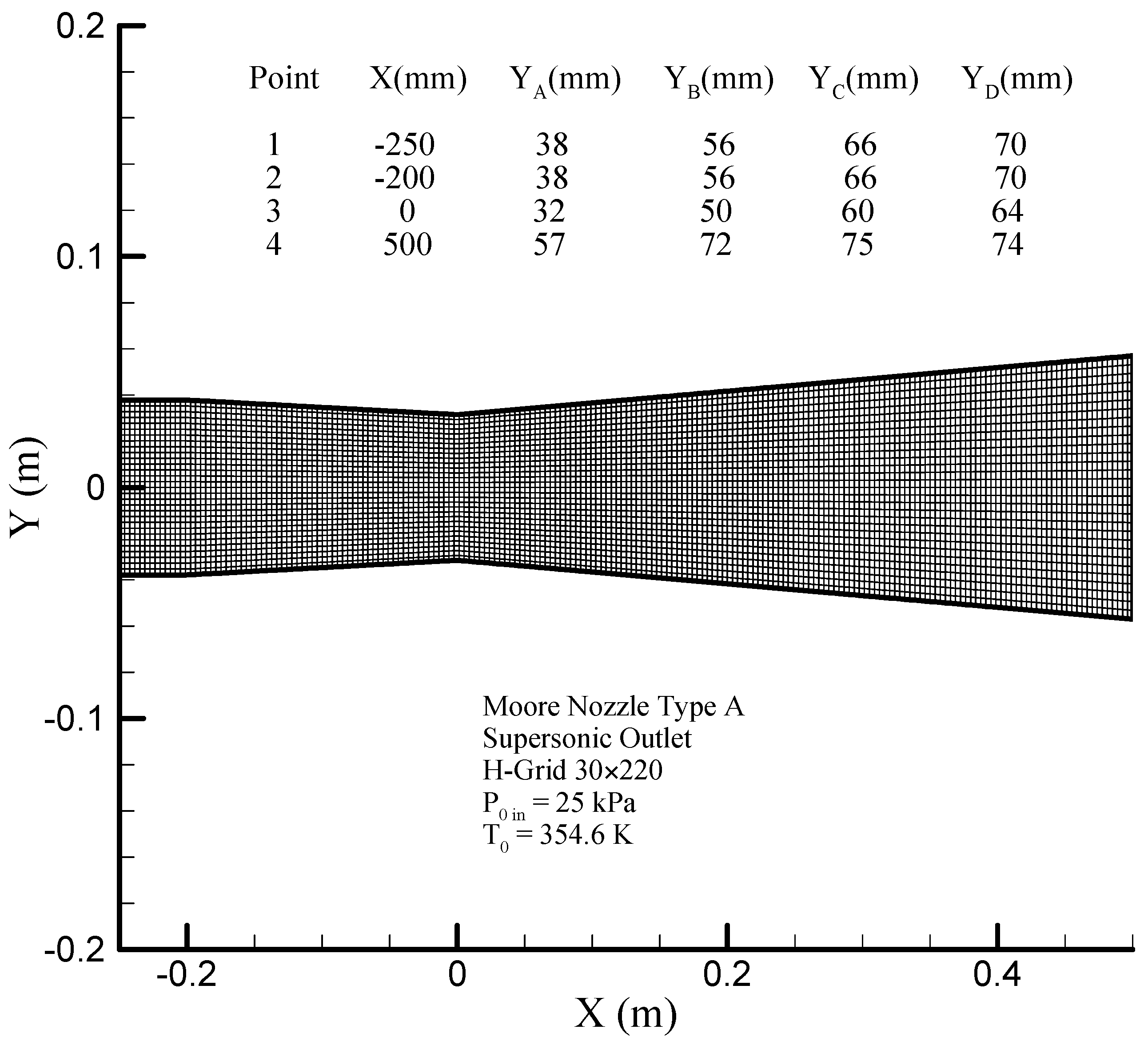
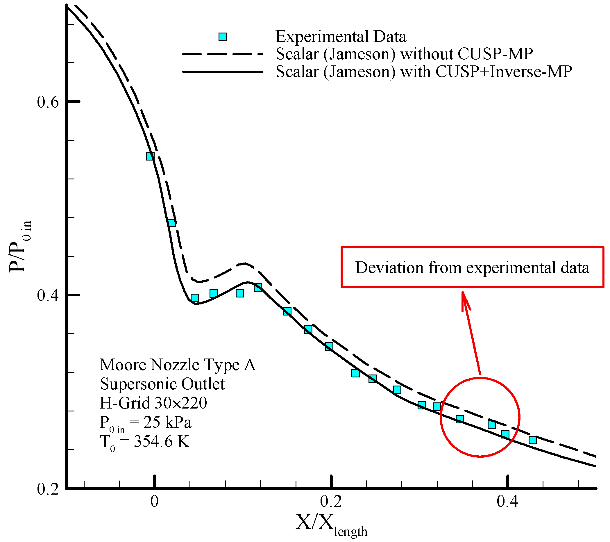
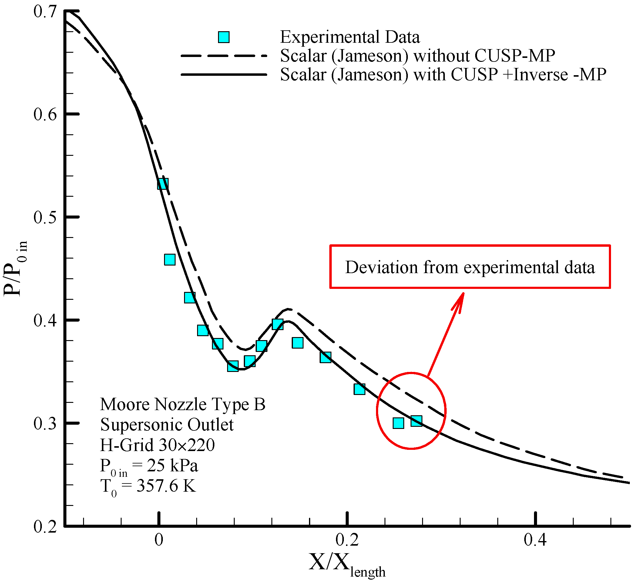
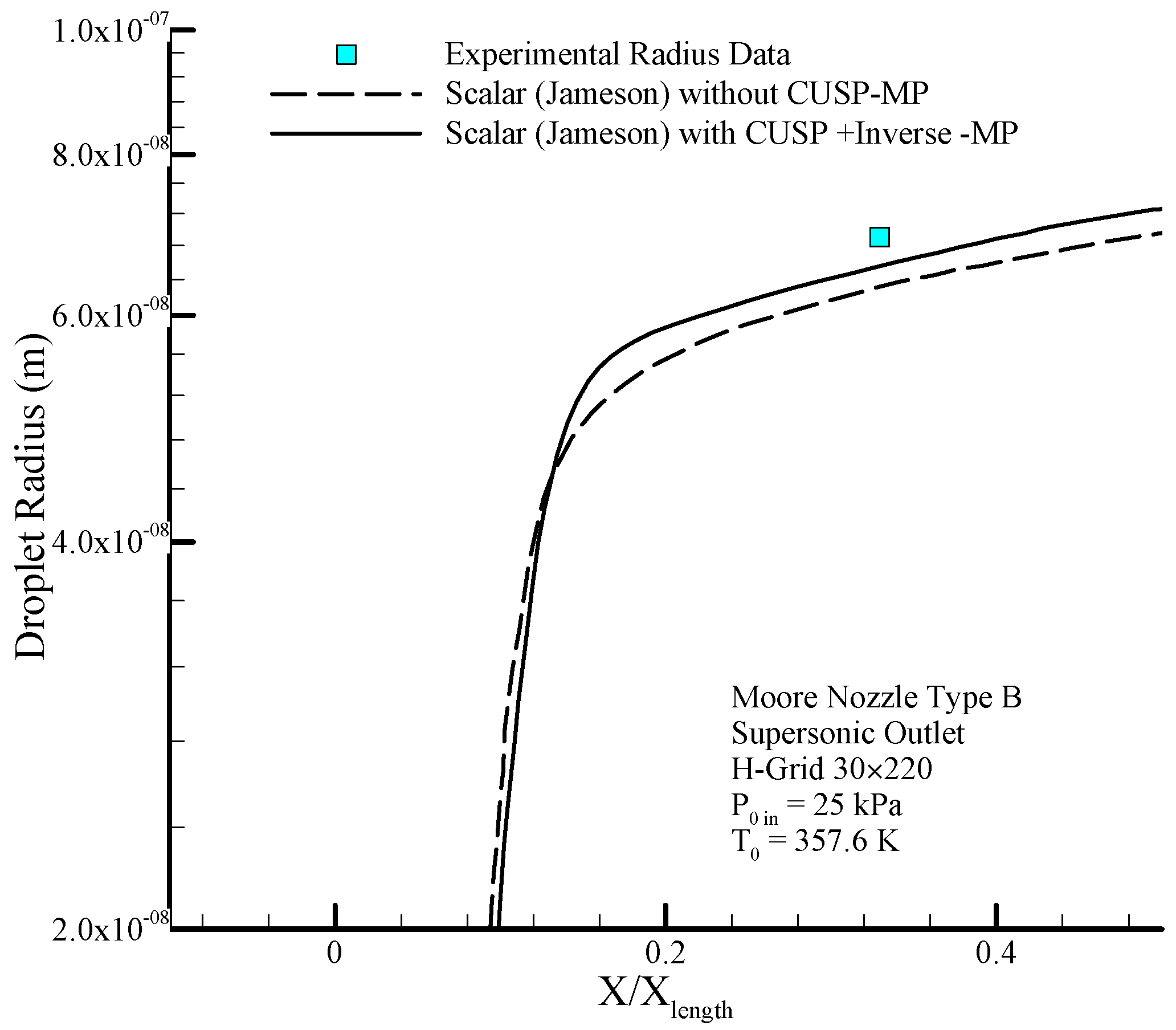
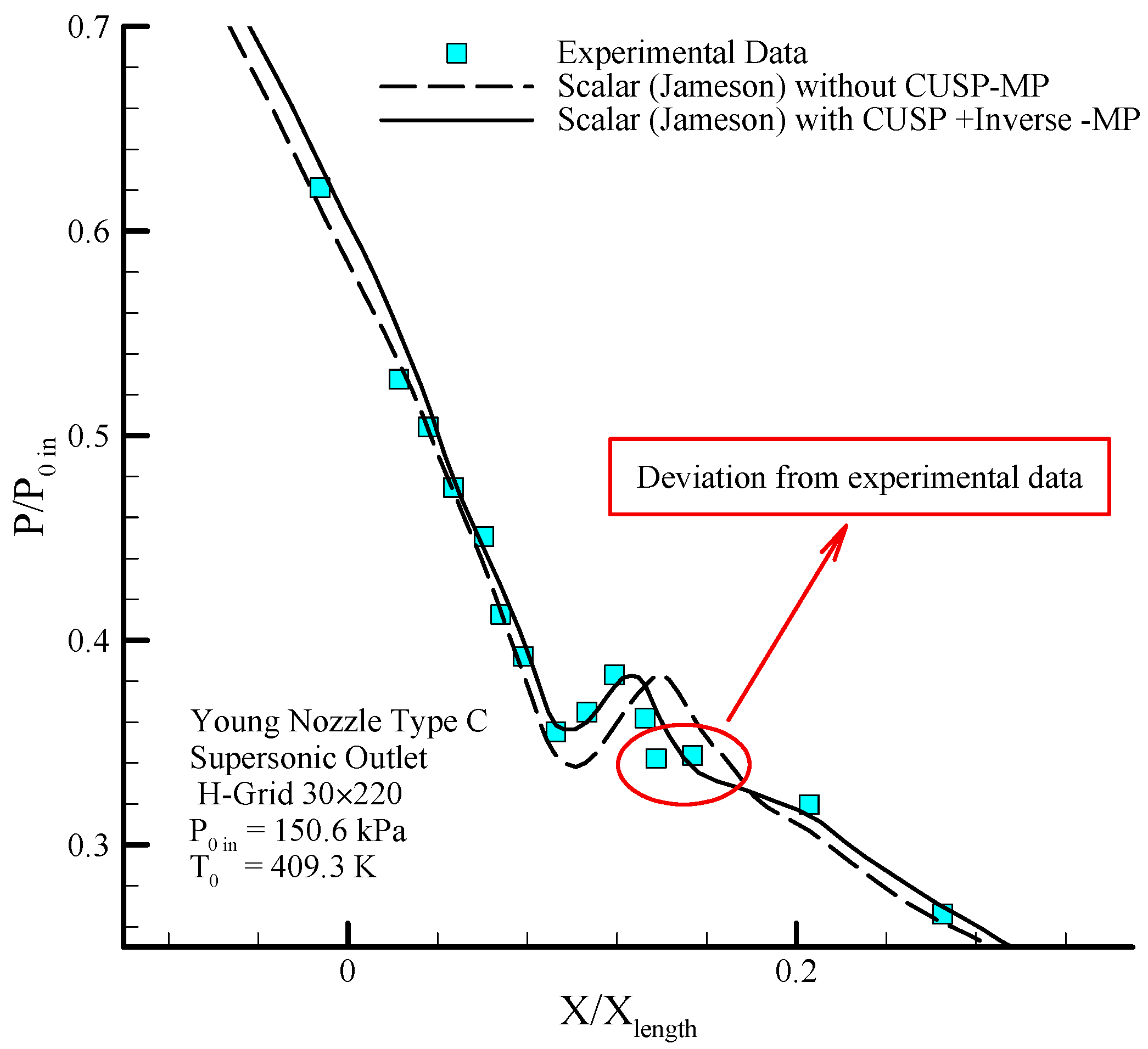
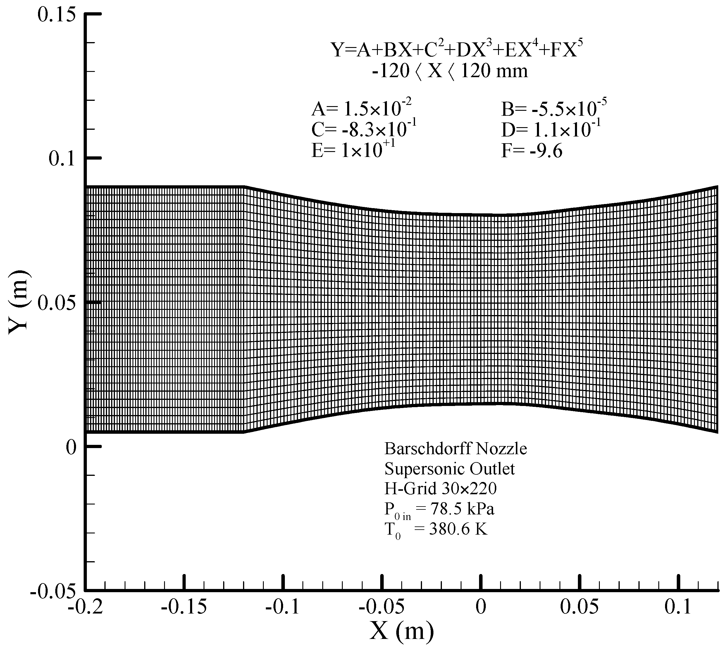
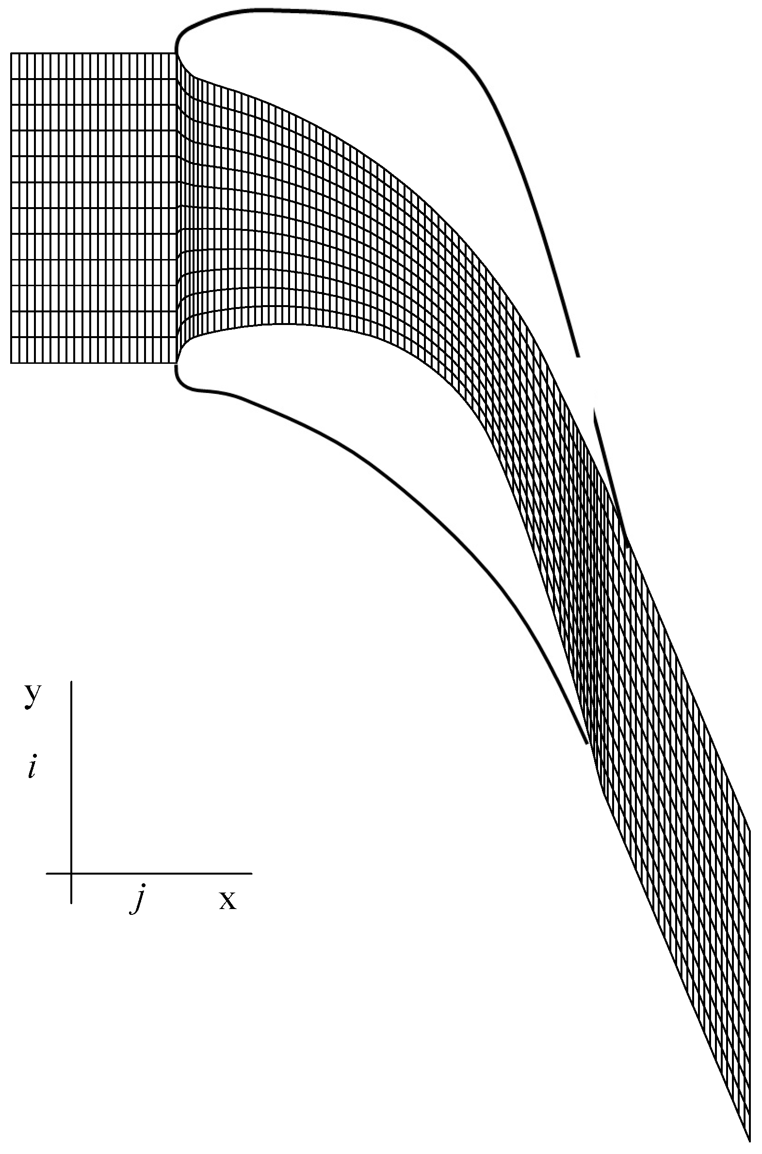
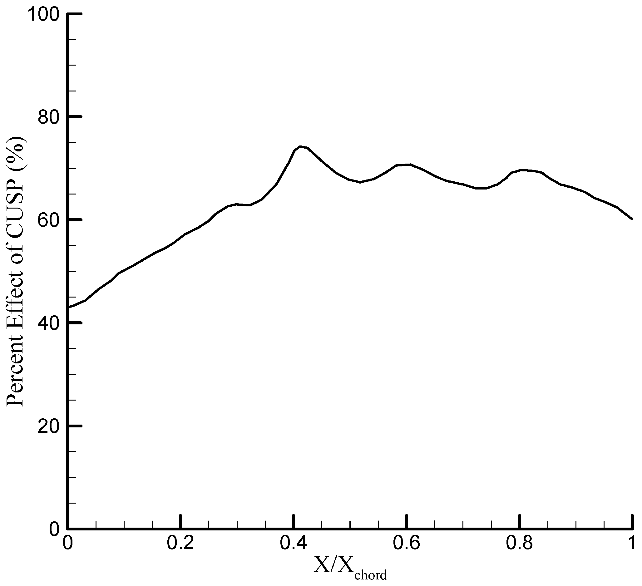
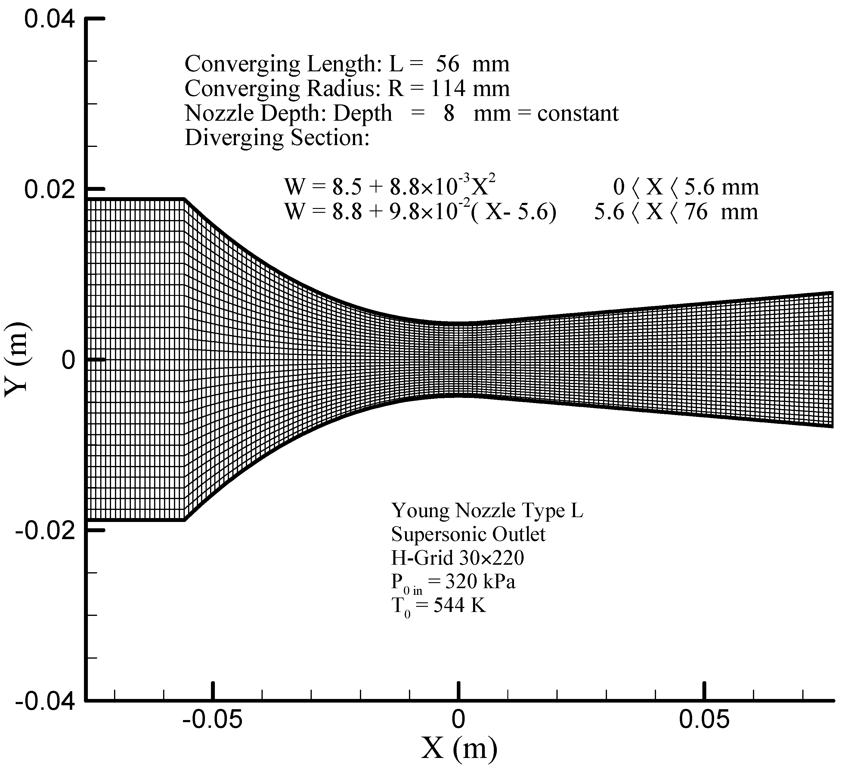
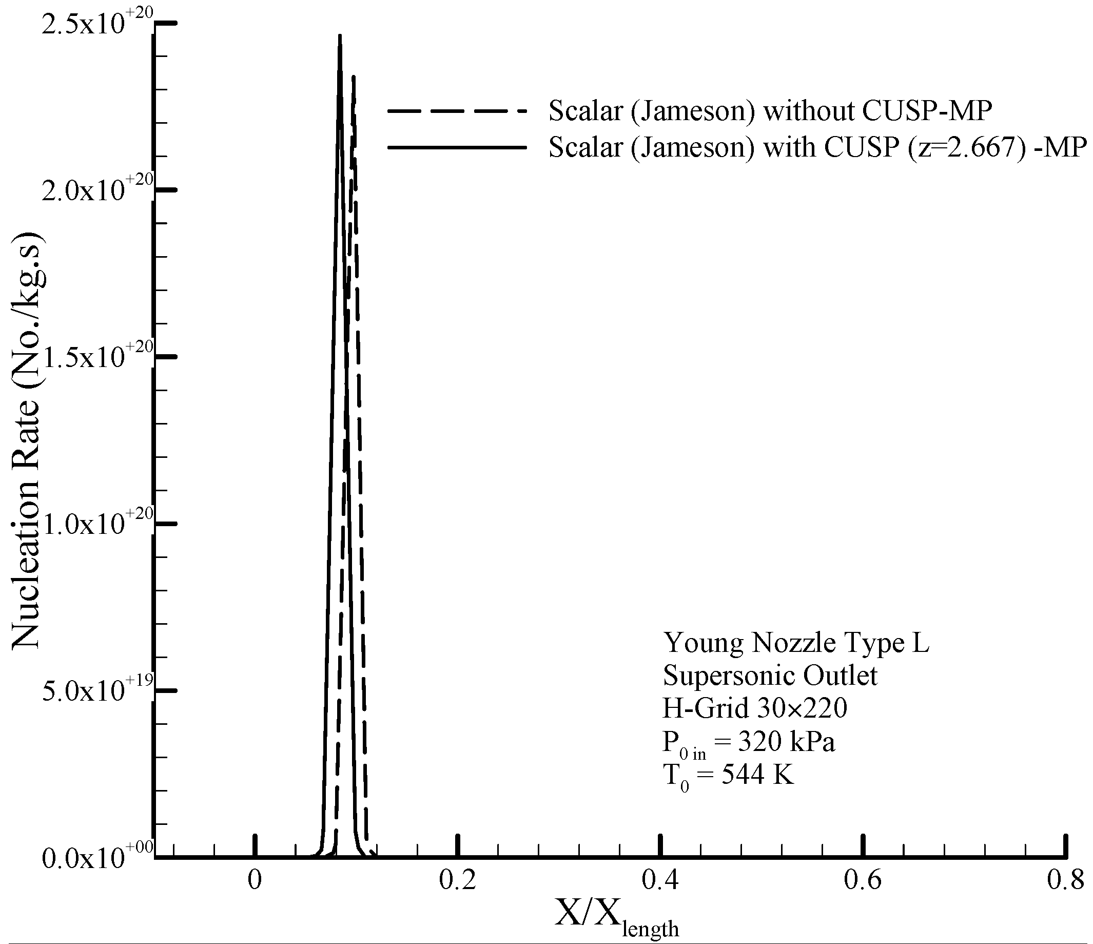
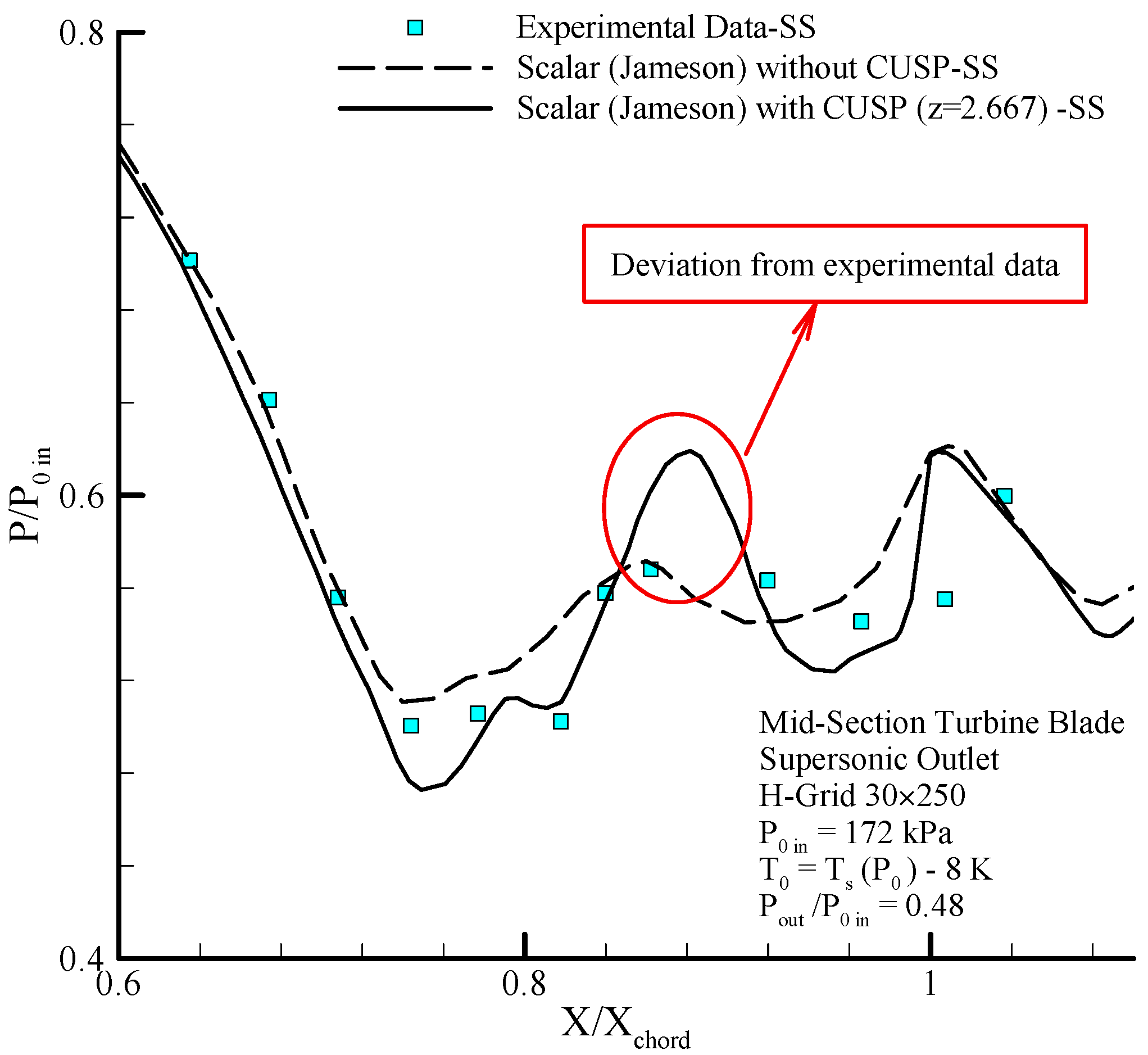
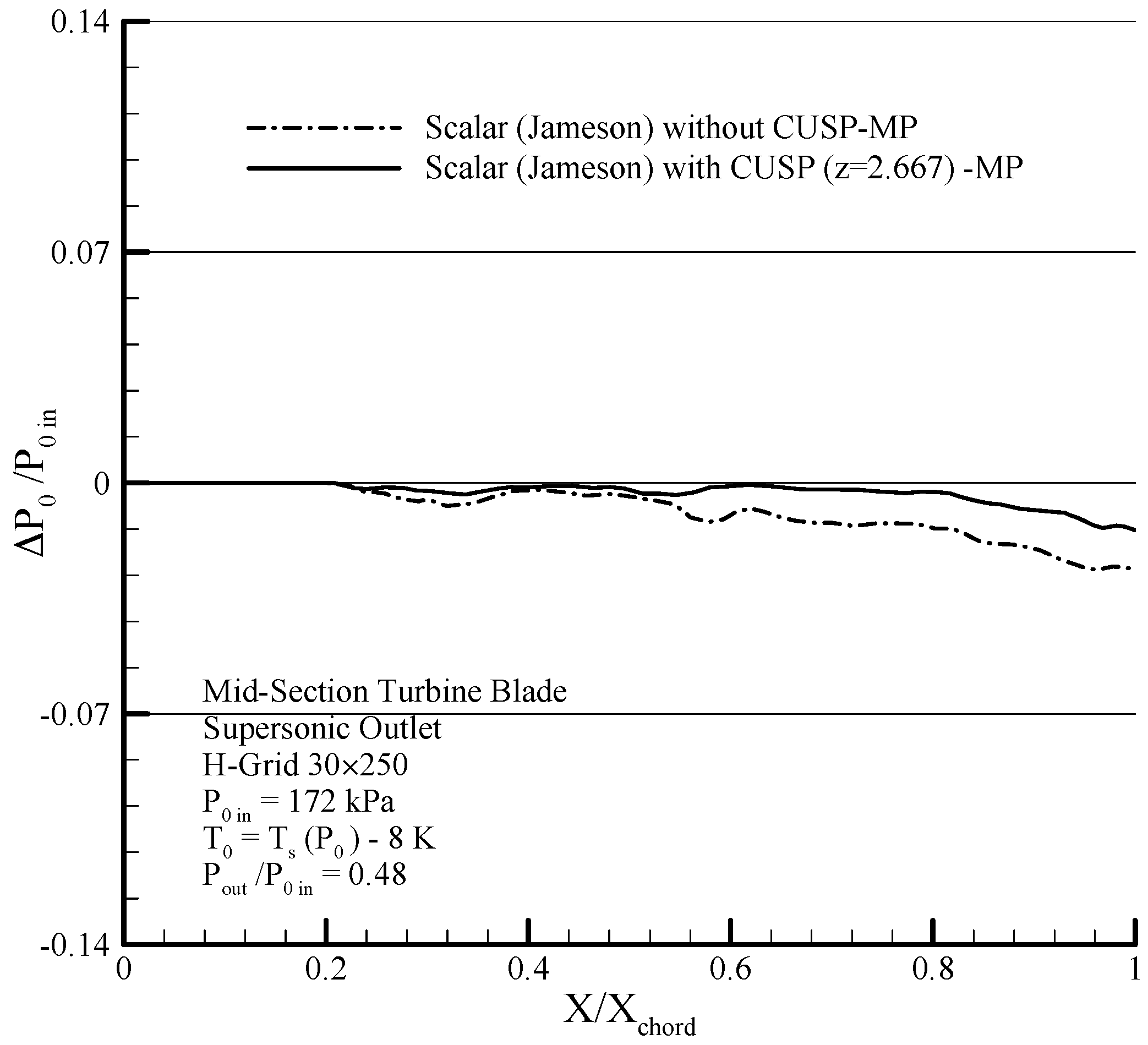
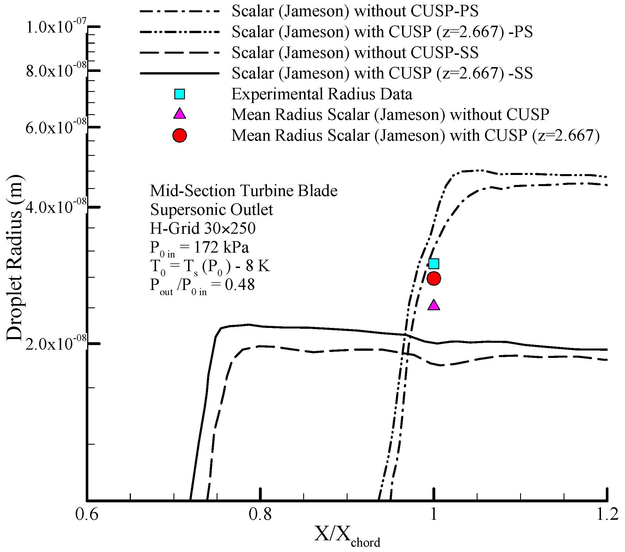
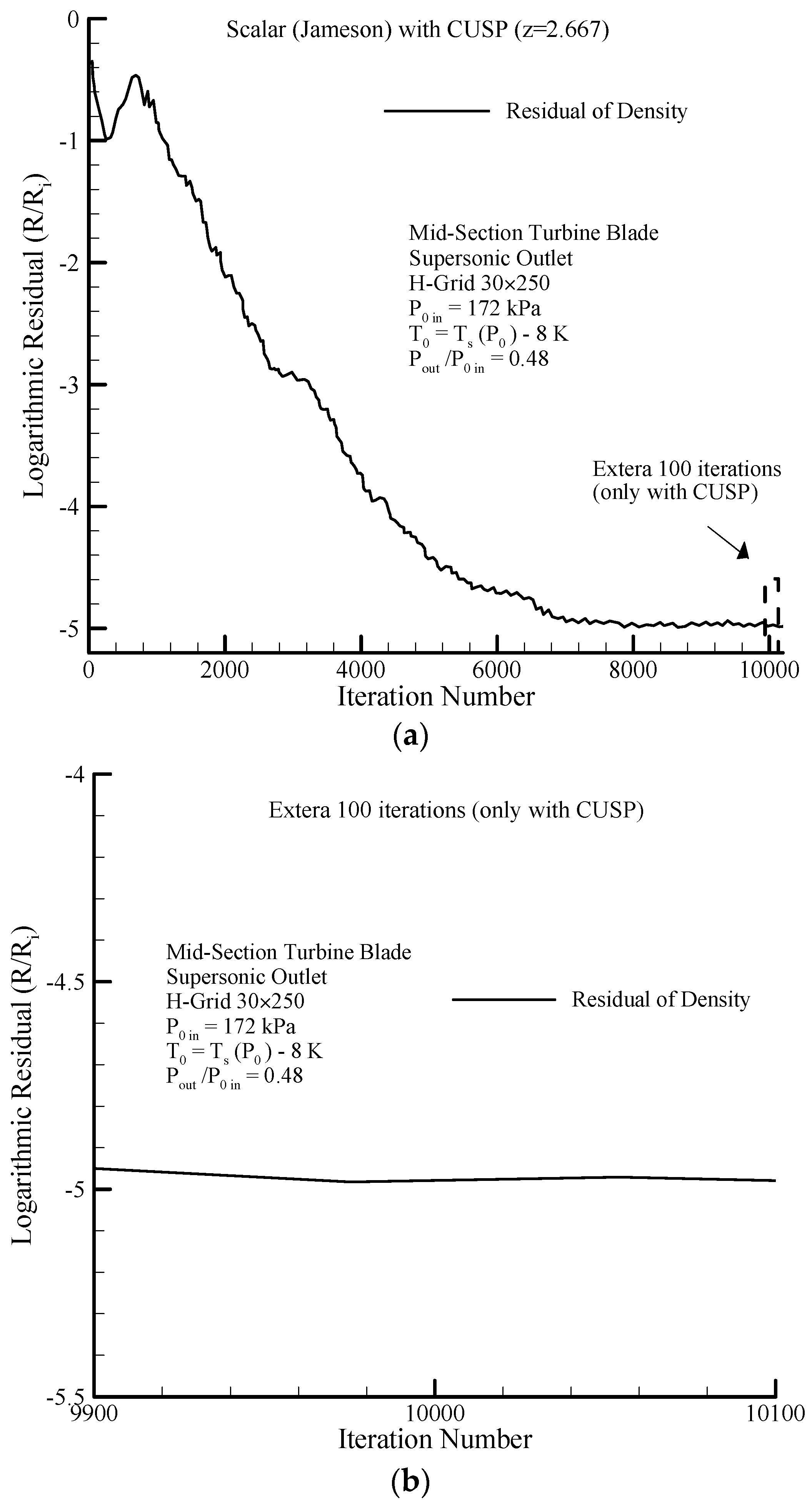
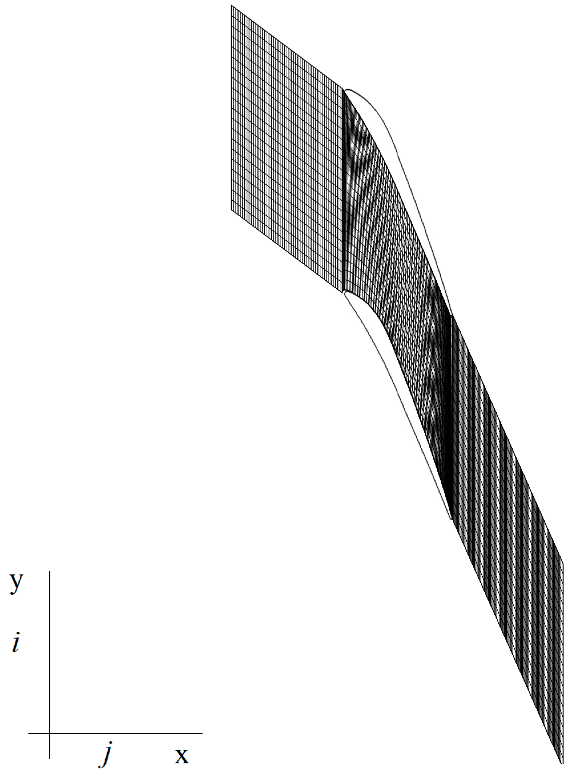
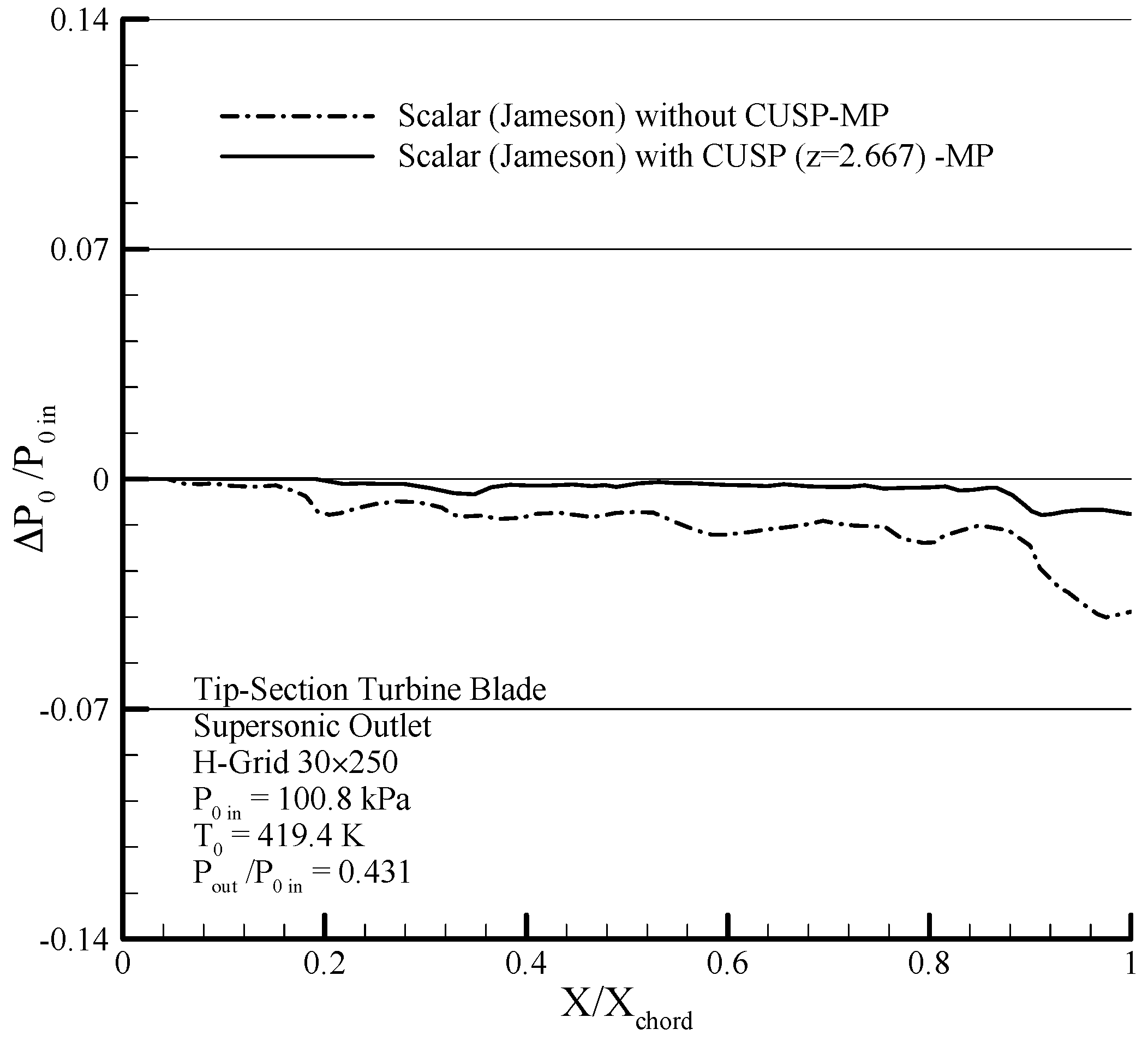
Table 1.
Boundary conditions for the three main cases.
| Geometry | Conditions | Mesh Size | Inlet Condition | Pressure Ratio | ||
|---|---|---|---|---|---|---|
| Young Nozzle Type (L) | 2D, Steady state, Supersonic outlet, Inviscid, Adiabatic Two-phase Flow | 30 × 220 | 320 | 544 | 6.7 | 0.43 |
| Mid-Section Turbine Blade | 30 × 250 | 172 | 654 | 8 | 0.48 | |
| Tip-Section Turbine Blade | 30 × 250 | 100.8 | 642 | 5.7 | 0.431 | |
© 2017 by the authors. Licensee MDPI, Basel, Switzerland. This article is an open access article distributed under the terms and conditions of the Creative Commons Attribution (CC BY) license (http://creativecommons.org/licenses/by/4.0/).
Share and Cite
MDPI and ACS Style
Yousefi Rad, E.; Mahpeykar, M.R. A Novel Hybrid Approach for Numerical Modeling of the Nucleating Flow in Laval Nozzle and Transonic Steam Turbine Blades. Energies 2017, 10, 1285. https://doi.org/10.3390/en10091285
AMA Style
Yousefi Rad E, Mahpeykar MR. A Novel Hybrid Approach for Numerical Modeling of the Nucleating Flow in Laval Nozzle and Transonic Steam Turbine Blades. Energies. 2017; 10(9):1285. https://doi.org/10.3390/en10091285
Chicago/Turabian StyleYousefi Rad, Edris, and Mohammad Reza Mahpeykar. 2017. "A Novel Hybrid Approach for Numerical Modeling of the Nucleating Flow in Laval Nozzle and Transonic Steam Turbine Blades" Energies 10, no. 9: 1285. https://doi.org/10.3390/en10091285
Note that from the first issue of 2016, this journal uses article numbers instead of page numbers. See further details here.