A Real-Time SOSM Super-Twisting Technique for a Compound DC Motor Velocity Controller

Abstract

In this paper, a real-time robust closed-loop control scheme for controlling the velocity of a Direct Current (DC) motor in a compound connection is proposed. This scheme is based on the state-feedback linearization technique combined with a second-order sliding mode algorithm, named super-twisting, for stabilizing the system and achieving control goals. The control law is designed to track a periodic square reference signal, being one of the most severe tests applied to closed-loop systems. The DC motor drives a squirrel-cage induction generator which represents the load; this generator must work above the synchronous velocity to deliver the generated power towards the grid. A classical proportional-integral (PI) controller is designed for comparison purposes of the time-domain responses with the proposed second-order sliding mode (SOSM) super-twisting controller. This robust controller uses only a velocity sensor, as is the case of the PI controller, as the time derivative of the velocity tracking variable is estimated via a robust differentiator. Therefore, the measurements of field current and stator current, the signal from a load torque observer, and machine parameters are not necessary for the controller design. The validation and robustness test of the proposed controller is carried out experimentally in a laboratory, where the closed-loop system is subject to an external disturbance and a time-varying tracking signal. This test is performed in real time using a workbench consisting of a DC motor—Alternating Current (AC) generator group, a DC/AC electronic drive, and a dSPACE 1103 controller board.

1. Introduction

To emulate a wind system in a lab application, a motor–generator couplet for reproducing the turbine operation can be used. The motors able to perform this task are the squirrel-cage induction motor, the permanent magnet synchronous motor, and the DC motor. It is important to point out that the DC motor can be set at a wide range of velocities operating in a maximum torque condition, which makes it the first option for the wind system emulator. A squirrel-cage induction generator is mechanically coupled to the DC motor working above synchonous velocity for delivering power to the grid. The power generated by the induction generator is fed directly into the grid without using any controller for it [1]. Controlling the DC motor speed in a sharp way can produce the effect of having a wind system connected in the lab, and the turbine power profile can be effectively obtained. In this regard, a robust, fast, reliable and cheap controller is needed for the DC motor. A closed-loop hysteresis regulator for emulating a wind turbine is illustrated in [2], where the armature current is controlled to regulate the DC motor electromagnetic torque. Here, if the error between the reference and the output exceeds the hysteresis upper limit, a negative voltage is applied to the DC motor armature. However, if the current error reaches the lower limit, a positive voltage is applied. A discontinuous control using sliding modes techniques with a non-linear sliding surface for robust disturbance rejection is exemplified in [3]. Linearization techniques by discrete-time block control combined with sliding modes and high-order neural networks are applied to track a velocity trajectory of a DC motor in [4]. The employment of an intelligent control method by fuzzy logic strategy is used to demonstrate how much the DC motor relies on the armature circuit or on the field circuit to produce the require velocity and is validated in [5]. An artificial controller based on a neural network model in order to keep the DC motor in the constant torque region is presented in [6]. Different applications using a super-twisting algorithm as a second-order sliding mode (SOSM) technique are reported in the literature. For example, an emulator of a scaled wind system, where a sliding surface is defined applying the block control linearization technique, combined with a super-twisting algorithm for controlling both the DC motor and a doubly-fed induction generator is exemplified in [7]. In [8], the super-twisting algorithm is employed to control a doubly-fed induction generator-based wind turbine, where the control objective is the maximization of power extraction, according to a bounded signal given by maximum power point tracking. Additionally, the upper bound of admissible unknown disturbances and the lower bound of the convergence time of the super-twisting algorithm are shown in [8]. Also, an adaptive super-twisting control algorithm for a two-degrees-of-freedom helicopter is presented in [9], where a nonlinear extended state observer is proposed for estimating the required non-measurable states, as well as parametric uncertainties and external disturbances. Another control strategy using the super-twisting algorithm is shown in [10,11]. In [11], the Lyapunov approach is applied to control a variable-speed wind system connected to the utility grid.

This paper proposes a robust SOSM super-twisting velocity controller applied to a compound DC motor. The main contributions are as follows. Firstly, the design of the sliding surface does not depend on the machine parameters, only depending on velocity measurement due to the application of a SOSM super-twisting differentiator for estimating the time derivative of the velocity error variable. Therefore, the SOSM super-twisting controller proposed in this work does not depend on the plant parameters as a classical proportional-integral (PI) controller does. Secondly, regarding a stability procedure obtained from the literature, the convergence ranges of controller gains in order to guarantee the robustness of the complete closed-loop system are obtained. Thirdly, real-time experiments are performed in a laboratory to validate the SOSM super-twisting velocity controller proposed using a machine group composed of a DC motor coupled to a squirrel-cage induction generator. Two-step severe simultaneous external disturbances are set up: a pulse train signal above synchronous velocity as reference signal and a pulse train of variations on the load torque, developed by the induction generator. Finally, the standard parameters (overshoot, rise time, falling time and settling time) of the time-domain responses to the PI controller and the SOSM super-twisting controller, with and without differentiators, are quantified and compared for assessment of the proposed controller.

This paper is organized in the following form: Section 2 introduces the compound DC motor mathematical model; the state-feedback linearization technique is described in Section 3; the design of the classical PI controller is explained in Section 4; the second-order sliding modes super-twisting algorithm is presented in Section 5; a robust differentiator to estimate de derivative of velocity tracking error is designed in Section 6; experimental results are provided in Section 7; and finally, conclusions are given in Section 8.

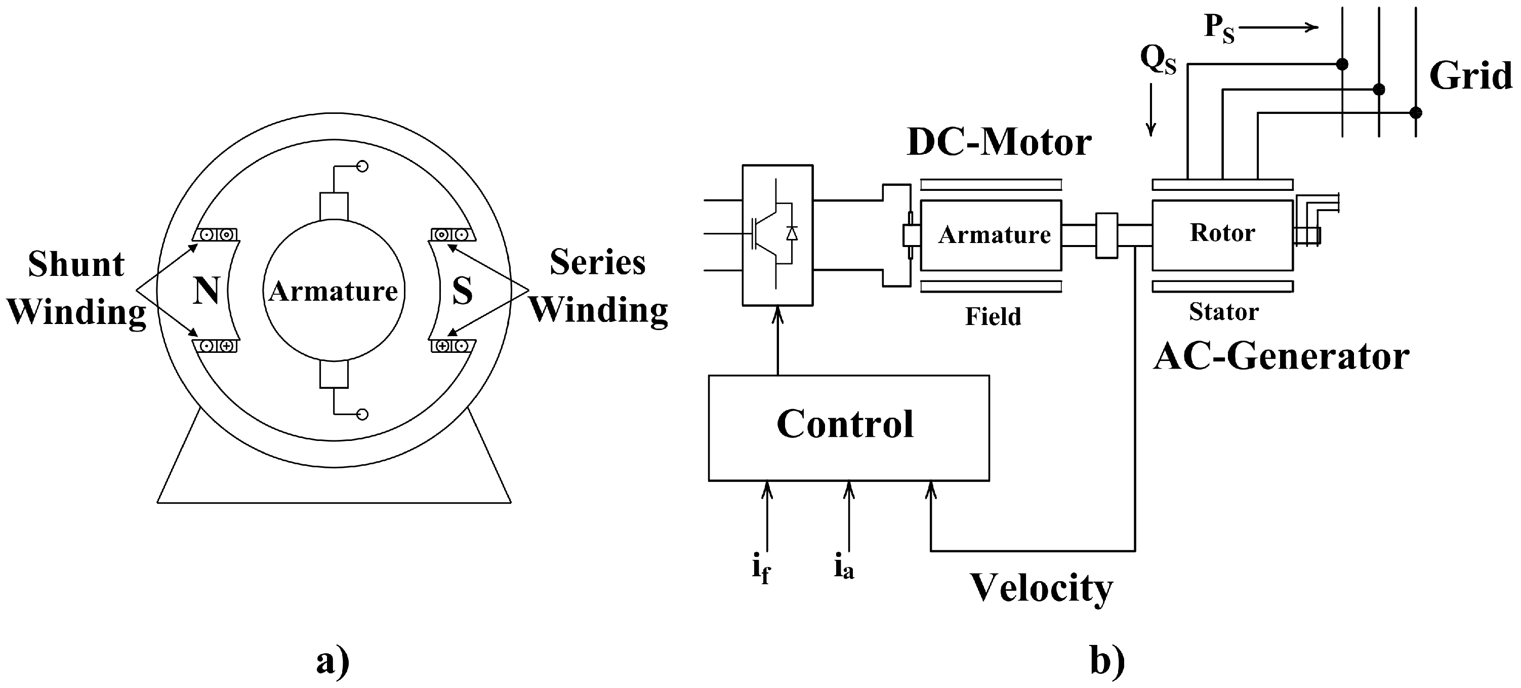
2. Direct Current Motor Mathematical Model

The DC motor is an energy conversion device from electrical input to mechanical output with many years of evolution in its manufacturing history. This machine is very versatile, and it is possible to perform several connection configurations of the field windings and then establish different operating characteristics. Using the DC motor as the prime motor, a wide range of velocities can be set. By modulating the voltage applied to armature winding, the DC motor works from rest to nominal velocity, and by weakening the machine’s field, winding velocities over those rated could be achieved. The DC motor with compound connection is composed of an armature winding which is mounted in slots of iron core laminations on the shaft, a shunt (principal), a series of (auxiliary) field windings mounted in the slots’ stators, a set of brushes for external electrical connection, and an enclosure to protect and align the machine with the mechanical system to impell and direct the mechanical stress towards the base. The main parts of the DC motor are shown in Figure 1a.

The mathematical model for the compound DC motor is established from the rotatory movement equation involving the shaft masses and its support points, and applying the voltage equilibrium equation to the armature circuit, considering the two magnetomotive forces of the shunt and series field windings. It is a common practice to consider linearity between the effective field current $i_{eff}$ and its magnetizing flux produced ${\varphi }_m$ due to the airgap. Then, the compound DC motor model can be expressed in the following form:

$$\begin{array}{c}\begin{array}{c}\frac{d{\omega }_m}{dt}=-\frac{1}{{\tau }_m}{\omega }_m+\frac{K_m}{J_m}{i}_{eff}{i}_a-\frac{1}{J_m}{T}_L,\hfill \\ \frac{d{i}_a}{dt}=-\frac{K_f}{L_T}{i}_{eff}{\omega }_m-\frac{1}{{\tau }_T}{i}_a+\frac{1}{L_T}{u}_a,\hfill \end{array}\hfill \end{array}$$

(1)

with

$$i_{eff}=i_f\pm \frac{N_s}{N_f}{i}_a,$$

(2)

and

$${\tau }_m=\frac{J_m}{B_m};{\tau }_T=\frac{L_T}{R_T}=\frac{L_s+L_a}{R_s+R_a},$$

where ${\omega }_m$ and $i_a$ are the angular velocity and armature current as the state variables, respectively. $i_{eff}$ is an input to the system (1) which varies slightly according to the increase of armature current $i_a$. It is defined by the total effect of the magnetomotive forces established by the field current $i_f$ in the shunt winding (main field), and the armature current flowing in the series winding (auxiliary field) that can connect in an accumulative (plus sign) or differential (negative sign) form. $\frac{N_s}{N_f}$ is the turn ratio between the series and shunt windings; and $R_s$ and $L_s$ are the resistance and inductance of the series winding, respectively. $R_a$ and $L_a$ are the resistance and inductance of the armature winding, respectively. ${\tau }_T$ and ${\tau }_m$ are the electrical and mechanical time constants, respectively. $K_m$ and $K_f$ are the DC motor constants with the same value and different units, and both are established considering a linear ratio between the effective field current $i_{eff}$ and the resulting magnetic flux ($K_m$ defines the electromagnetic torque, while $K_f$ defines the induced voltage in the armature winding). $B_m$ represents the viscous friction coefficient at the support points, and $J_m$ denotes the moment of inertia to the masses involved at the shaft train. Model (1) is a second-order linear system with two electrical inputs: armature voltage $u_a$ and effective current $i_{eff}$, which is modeled as an external disturbance; and there is one mechanical input $T_L$ named the load torque which is also considered as an external disturbance. It is important to remark that the load torque is not measured by a sensor but estimated by an asymptotic observer, which is modeled as follows:

$$\begin{array}{c}\frac{d{\widehat{\omega }}_m}{dt}=-\frac{1}{{\tau }_m}{\widehat{\omega }}_m+\frac{K_m}{J_m}{i}_{eff}{i}_a-\frac{1}{J_m}{\widehat{T}}_L+l_1\left({\omega }_m-{\widehat{\omega }}_m\right),\hfill \\ \frac{d{\widehat{T}}_L}{dt}=l_2\left({\omega }_m-{\widehat{\omega }}_m\right),\hfill \end{array}$$

(3)

where $l_1$ and $l_2$ are constants defined to stabilize the observation error.

On the other hand, the DC motor velocity is controlled above the synchronous velocity in order to connect the induction generator directly to the grid. In this case, the induction generator represents the mechanical load for the DC motor. The developed power of the generator increases with the slip velocity which is the difference between the synchronous velocity and rotor velocity; therefore, when the speed goes up, the power delivered to the grid grows in a similar way. The block scheme for the DC motor velocity controller is shown in Figure 1b. The measured variables are the field and armature currents $i_f$ and $i_a$, and angular velocity ${\omega }_m$. Meanwhile, the effective current is calculated as indicated in (1) and the load torque is estimated by an asymptotic observer. The control signal $u_a$ is conditioned to feeding the armature circuit through the pulse width modulation (PWM) technique to activate the gates of the insulated gate bipolar transistors (IGBTs) which are arranged in “H" bridge converter. To quantify the delivered power by AC generator toward the grid, the currents in each phase and two line-to-line voltages at the bus are measured.

3. State Feedback Linearization

The state-feedback linearization technique can be applied both linear and non-linear systems. It consists of applying a similitude transformation to a dynamic system for obtaining an equivalent linear system with new state variables. A control law is then designed to relocate the eigenvalues in the new linear system. This new system representation is named control canonical form as to each state variable has a connection directly with the control input through the feedback branch.

Consider a single-input single-output (SISO) linear system in a control canonical form defined by [12]:

$$\begin{array}{c}\hfill \begin{array}{c}{\dot{x}}_1=x_2\hfill \\ {\dot{x}}_2=x_3\hfill \\ ⋮\hfill \\ {\dot{x}}_{n-1}=x_n\hfill \\ {\dot{x}}_n=-b_0{x}_1-b_1{x}_2-\cdots -b_{n-2}{x}_{n-1}-b_{n-1}{x}_n+g(x,t)+u\hfill \\ y=a_0{x}_1+a_1{x}_2+\cdots +a_{n-2}{x}_{n-1}+a_{n-1}{x}_n\hfill \end{array}\end{array}$$

(4)

where u and y represent the input and output of the system, respectively; $x_n$ denotes the n-$th$ plant state variables; n is the state dimension; the coefficients $a_k$ and $b_k$, $k=1,2,\dots ,n-1$ represent parameters of the plant; and $g(x,t)$ is a smooth and bounded function and it models the external disturbances and parameter variation.

Let us start the feedback linearization technique to represent the DC motor model (1) into the control canonical form (4), by defining a new variable error ${\epsilon }_1$ as:

$${\epsilon }_1={\omega }_{ref}-{\omega }_m,$$

(5)

where ${\omega }_{ref}$ represents the reference signal to be tracked and ${\omega }_m$ is the DC motor velocity. Upon differentiating Equation (5), and based on system (1), the velocity error dynamics takes the form:

$${\dot{\epsilon }}_1={\dot{\omega }}_{ref}+\frac{1}{{\tau }_m}{\omega }_m-\frac{K_m{i}_{eff}}{J_m}{i}_a+\frac{1}{J_m}{T}_L.$$

(6)

Define a new state variable error ${\epsilon }_2$ as the first time derivative of ${\epsilon }_1$:

$${\epsilon }_2={\dot{\epsilon }}_1.$$

(7)

Taking its first derivative, involving system (1), results in:

$${\dot{\epsilon }}_2=\frac{d^2{\omega }_{ref}}{d{t}^2}+\frac{1}{{\tau }_m}\frac{d{\omega }_m}{dt}-\frac{K_m{i}_{eff}}{J_m}\frac{d{i}_a}{dt}+\frac{1}{J_m}\frac{d{T}_L}{dt},$$

(8)

and solving for the armature current $i_a$ from (6) and involving (5), results in:

$$i_a=\frac{B_m}{K_m{i}_{eff}}\left({\omega }_{ref}-{\epsilon }_1\right)-\frac{J_m}{K_m{i}_{eff}}{\epsilon }_2+\frac{J_m}{K_m{i}_{eff}}{\dot{\omega }}_{ref}+\frac{1}{K_m{i}_{eff}}{T}_L.$$

(9)

Using (1), (5) and (9) into (8), replacing $K_m$ with $K_f$ for simplicity of operation as they have the same values, the control canonical form of the DC motor model results are as follows:

$$\begin{array}{cc}{\dot{\epsilon }}_1=\hfill & {\epsilon }_2\hfill \\ {\dot{\epsilon }}_2=\hfill & -\left(\frac{K_f^2{i}_{eff}^2}{J_m{L}_T}+\frac{1}{{\tau }_T{\tau }_m}\right){\epsilon }_1-\left(\frac{1}{{\tau }_T}+\frac{1}{{\tau }_m}\right){\epsilon }_2\hfill \\ & +{\ddot{\omega }}_{ref}+\left(\frac{1}{{\tau }_T}+\frac{1}{{\tau }_m}\right){\dot{\omega }}_{ref}+\left(\frac{K_f^2{i}_{eff}^2}{J_m{L}_T}+\frac{1}{{\tau }_T{\tau }_m}\right){\omega }_{ref}\hfill \\ & +\frac{1}{J_m}{\dot{T}}_L+\frac{1}{J_m{\tau }_T}{T}_L-\frac{K_f{i}_{eff}}{J_m{L}_T}{u}_a.\hfill \end{array}$$

(10)

System (10) has the following characteristics: (a) it is equivalent to a compound DC motor model (1) with the same modes of operation (eigenvalues); (b) the ratio between the effective field current $i_{eff}$ (2) and the produced magnetizing flux ${\varphi }_m$ is nonlinear in real-time applications; (c) the effective current $i_{eff}$, being a system input, has small variations around the constant shunt field current (main field) due to the armature current variations that flow in the series winding (auxiliary field); (d) the DC motor is subject to parameter variations, for example: changes of armature resistance by temperature variations; (e) the procedure of machine parameter identification is uncertain; (f) the reference signal, as an external disturbance, is a periodic square signal (pulse train) above synchronous velocity, being one of the most severe disturbances applied to closed-loop systems; and (g) the load torque, as an external disturbance, varies in a pulse train form according to the slip velocity of the induction generator that delivers power to the utility grid. Taking into account the aforementioned characteristics, we can consider the DC motor as a complex system. From the control canonical form (10), the control law $u_a$ rejects the external perturbations ($T_L$ and ${\dot{T}}_L$), and cancels the reference velocity ${\omega }_{ref}$ and its first and second time derivatives; furthermore, the control law stabilizes the system with faster eigenvalues and steers the two error variables ${\epsilon }_1$ and ${\epsilon }_2$ asymptotically to zero in finite time; therefore, the system (10) becomes:

$$\left[\begin{array}{c}{\dot{\epsilon }}_1\\ {\dot{\epsilon }}_2\end{array}\right]=\left[\begin{array}{cc}0& 1\\ -K_1& -K_2\end{array}\right]\left[\begin{array}{c}{\epsilon }_1\\ {\epsilon }_2\end{array}\right],$$

(11)

and choosing constants $K_1>0$ and $K_2>0$, the closed loop system (11) is asymptotically stable.

Once system (11) is achieved through the control law $u_a$, the new eigenvalues are calculated by the following determinant:

$$\det \left(s\left[\begin{array}{cc}1& 0\\ 0& 1\end{array}\right]-\left[\begin{array}{cc}0& 1\\ -K_1& -K_2\end{array}\right]\right)=s^2+K_{2}s+K_1=0,$$

(12)

and these eigenvalues are related with the stable dynamics $K_1$ and $K_2$ through quantifying the roots of (12) with the following equations:

$$\begin{array}{c}\hfill \begin{array}{cc}\hfill p_1=& \frac{K_1}{p_2},\hfill \\ \hfill p_2=& \frac{K_2}{2}+\sqrt{{\left(\frac{K_2}{2}\right)}^2-K_1},\hfill \end{array}\end{array}$$

(13)

where $p_1$ and $p_2$ meet $\mathrm{Re}\left[p_i\right]>0$ and denote the specified eigenvalues of the closed-loop system (11) being faster than the eigenvalues of open-loop system (1); so the dynamic system’s response (11) is faster than the response of system (1).

4. Classical PI Controller

This section introduces the classical proportional-integral ($PI$) controller. The $PI$ algorithm as a standard control law is obtained directly from the velocity tracking error variable. It consists of proportional and integral terms, and is represented as follows:

$$u_a=K_p{\epsilon }_1+K_i\int {\epsilon }_{1}dt,$$

(14)

where $K_p$ is a constant gain at the proportional term to the velocity error variable ${\epsilon }_1$, and $K_i$ is a constant gain at the integral term of the error variable ${\epsilon }_1$. The proportional term, $K_p{\epsilon }_1$ acts with enough energy to stabilize the velocity error ${\epsilon }_1$ and steers it to zero in finite time even in the presence of external disturbances or changes in the reference signal. The system with only proportional control usually presents a steady-state offset which gets smaller as the gain is increased. To overcome this difficulty, the integral term $K_i\int {\epsilon }_{1}dt$ makes sure the steady state offset is eliminated, and consequently the velocity error variable ${\epsilon }_1$ remains closed to zero. The feedback system (10) with disturbances involving the PI controller takes the following form:

$$\begin{array}{cc}\left[\begin{array}{c}{\dot{\epsilon }}_0\\ {\dot{\epsilon }}_1\\ {\dot{\epsilon }}_2\end{array}\right]=\hfill & \left[\begin{array}{ccc}0& 1& 0\\ 0& 0& 1\\ -\frac{K_f{i}_{eff}}{J_m{L}_T}{K}_i& -\left(\frac{K_f^2{i}_{eff}^2}{J_m{L}_T}+\frac{1}{{\tau }_T{\tau }_m}+\frac{K_f{i}_{eff}}{J_m{L}_T}{K}_p\right)& -\left(\frac{1}{{\tau }_T}+\frac{1}{{\tau }_m}\right)\end{array}\right]\left[\begin{array}{c}{\epsilon }_0\\ {\epsilon }_1\\ {\epsilon }_2\end{array}\right]\hfill \\ & +\left[\begin{array}{ccc}0& 0& 0\\ 0& 0& 0\\ 1& \left(\frac{1}{{\tau }_T}+\frac{1}{{\tau }_m}\right)& \frac{1}{J_m}\end{array}\right]\left[\begin{array}{c}{\ddot{\omega }}_{ref}\\ {\dot{\omega }}_{ref}\\ {\dot{T}}_L\end{array}\right]+\left[\begin{array}{cc}0& 0\\ 0& 0\\ \left(\frac{K_f^2{i}_{eff}^2}{J_m{L}_T}+\frac{1}{{\tau }_T{\tau }_m}\right)& \frac{1}{J_m{\tau }_T}\end{array}\right]\left[\begin{array}{c}{\omega }_{ref}\\ T_L\end{array}\right]\hfill \end{array}$$

(15)

where its characteristic polynomial by applying Equation (12) into (15) results in:

$${\lambda }^3+\left(\frac{1}{{\tau }_T}+\frac{1}{{\tau }_m}\right){\lambda }^2-\left(\frac{K_f^2{i}_{eff}^2}{J_m{L}_T}+\frac{1}{{\tau }_T{\tau }_m}+\frac{K_f{i}_{eff}}{J_m{L}_T}{K}_p\right)\lambda +\frac{K_f{i}_{eff}}{J_m{L}_T}{K}_i=0.$$

(16)

Using Routh’s stability criterion [12], the control gains $K_i$ and $K_p$ must meet the following constraints:

$$K_i>0,$$

(17)

and,

$$K_p>\frac{{\tau }_m{\tau }_T}{{\tau }_m+{\tau }_T}{K}_i-\frac{B_m{R}_T}{K_f{i}_{eff}}-K_f{i}_{eff}.$$

(18)

Once inequalities (17) and (18) meet, the closed system (15) is asymptotically stable.

5. Second-Order Sliding Mode Super-Twisting Controller

The sliding mode is a robust control technique based on variable structure systems for controlling non-linear closed-loop systems operating under uncertain conditions. The sliding mode technique has the property of reducing the order system through the sliding surface design involving the system variables; this surface is the argument of a discontinuous control law. This control input commutes at high frequency, ensuring a motion of the state variables towards the sliding surface. This motion is called the sliding mode [13]. These characteristics are related with the first-order sliding mode (FOSM).

The high frequency commutation of FOSM produces a chattering effect which is characterized by dangerous high-frequency vibrations of the controlled system. In order to reduce the chattering effect, second-order sliding modes (SOSMs) are an alternative technique, which use the basic FOSM idea but act in both the sliding surface and its first derivative.

A very effective SOSM technique applied in closed-loop systems is the super-twisting algorithm which is applicable to a system where control appears in the first derivative of the sliding variable [14,15]. The super-twisting algorithm has the following advantages: (1) it compensates uncertainties that are Lipschitz; (2) it requires only information of the sliding variable; (3) it provides finite-time convergence to the origin for the sliding variable and its time derivative simultaneously; and (4) it generates continuous control signals and reduces the chattering [15].

In this proposal, the state feedback linearization technique is combined with the SOSM super-twisting algorithm to achieve robustness in the velocity tracking controller design. By applying the linearization technique, a sliding variable s is designed which is the argument of the super-twisting algorithm as the control law. The control canonical form (10) has a relative degree of two; then, in order to reduce the relative degree of system (10) and to set a robust closed-loop system, the following transformation is proposed:

$$s=C_1{\epsilon }_1+{\epsilon }_2,$$

(19)

where its first-order dynamics, involving system (10), result in:

$$\dot{s}=\rho -K_v{u}_a,$$

(20)

where:

$$\begin{array}{cc}\rho =\hfill & -\left(\frac{K_f^2{i}_{eff}^2}{J_m{L}_T}+\frac{1}{{\tau }_T{\tau }_m}\right){\epsilon }_1-\left(\frac{1}{{\tau }_T}+\frac{1}{{\tau }_m}-C_1\right){\epsilon }_2\hfill \\ & +{\ddot{\omega }}_{ref}+\left(\frac{1}{{\tau }_T}+\frac{1}{{\tau }_m}\right){\dot{\omega }}_{ref}+\left(\frac{K_f^2{i}_{eff}^2}{J_m{L}_T}+\frac{1}{{\tau }_T{\tau }_m}\right){\omega }_{ref}\hfill \\ & +\frac{1}{J_m}{\dot{T}}_L+\frac{1}{J_m{\tau }_T}{T}_L,\hfill \end{array}$$

and

$$K_v=\frac{K_f{i}_{eff}}{J_m{L}_T}.$$

To stabilize system (20) and steer the sliding variable s to the origin, the super-twisting control algorithm is applied [14]:

$$u_a=\lambda {\left|s\right|}^{1/2}\mathrm{sign}s+{\int }_0^t\alpha \mathrm{sign}s\left(\tau \right)d\tau .$$

(21)

By applying the control law $u_a$ (21) in new system (20), the sliding variable s steers toward zero in finite time with an asymptotically stable movement of ${\dot{\epsilon }}_1=-C_1{\epsilon }_1$, where $C_1$ is a new eigenvalue, and its value can be greater than the two eigenvalues in the open-loop operation of the compound DC motor. $C_1$ is restricted by the amount of energy of the actuator and the rated voltage of the DC motor. To define the range of the control gains, $\lambda$ and $\alpha$ for which the closed-loop system (20) is stable, we have reviewed reference [16,17], where a Lyapunov function is proposed to study more deeply the convergence of the super-twisting algorithm when strong disturbances are present. System (20) with control law (21) can be represented as follows:

$$\begin{array}{c}\hfill \begin{array}{c}\dot{s}=-K_v\lambda {\left|s\right|}^{1/2}\mathrm{sign}\left(s\right)+s_1+\rho ,\hfill \\ {\dot{s}}_1=-K_v\alpha \mathrm{sign}\left(s\right),\hfill \end{array}\end{array}$$

(22)

By simplifying (22), this closed-loop system can be presented as:

$$\begin{array}{c}\hfill \begin{array}{c}\dot{s}=-k_1{\left|s\right|}^{1/2}\mathrm{sign}\left(s\right)+s_1+\rho ,\hfill \\ {\dot{s}}_1=-k_2\mathrm{sign}\left(s\right),\hfill \end{array}\end{array}$$

(23)

where:

$$\begin{array}{c}\hfill \begin{array}{c}{k}_1=K_v\lambda ,\hfill \\ k_2=K_v\alpha .\hfill \end{array}\end{array}$$

(24)

Applying the following transformation proposed by [16,17,18]:

$$\varsigma ={\left[\begin{array}{cc}{\left|s\right|}^{1/2}\mathrm{sign}\left(s\right)& s_1\end{array}\right]}^{\top },$$

(25)

and its time derivative:

$$\dot{\varsigma }=\frac{1}{|{\varsigma }_1|}{\left[\begin{array}{cc}\frac{1}{2}\left(-k_1{\varsigma }_1+{\varsigma }_2+\rho \right)& -k_2{\varsigma }_1\end{array}\right]}^{\top },$$

(26)

where:

$$|{\varsigma }_1{|=|s|}^{1/2}.$$

System (23) can be represented in linear form as follows:

$$\dot{\varsigma }=\frac{1}{|{\varsigma }_1|}\left(\mathbf{A}\varsigma +\rho \right)$$

(27)

where:

$$\mathbf{A}=\left[\begin{array}{cc}-{\displaystyle \frac{1}{2}}{k}_1& {\displaystyle \frac{1}{2}}\\ -k_2& 0\end{array}\right]\mathrm{and}\rho =\left[\begin{array}{c}{\displaystyle \frac{1}{2}}\rho \\ 0\end{array}\right],$$

and the external disturbance $\rho$ is bounded by:

$$\left|\rho \right|={\delta \left|s\right|}^{1/2},\delta >0.$$

(28)

To analyse stability condition for system (27), we apply the following candidate Lyapunov function [16,17,18]:

$$V\left(\varsigma \right)={\varsigma }^{\top }\mathbf{P}\varsigma ,$$

(29)

where:

$$\mathbf{P}=\frac{1}{2}\left[\begin{array}{cc}4k_2+k_1^2& -k_1\\ -k_1& 2\end{array}\right].$$

Taking the derivative of the candidate Lyapunov function results in:

$$\dot{V}\left(\varsigma \right)=\frac{1}{|{\varsigma }_1|}{\varsigma }^{\top }\left({\mathbf{A}}^{\top }\mathbf{P}+\mathbf{P}\mathbf{A}\right)\varsigma +\frac{2}{|{\varsigma }_1|}{\varsigma }^{\top }\mathbf{P}\rho .$$

(30)

Assume that the external disturbance $\rho$ satisfies the following bound:

$$\rho =\delta |s_0{|}^{1/2}\mathrm{sign}\left(s_0\right)=\delta {\varsigma }_1.$$

(31)

Substituting (31) into the second term of (30) and grouping terms yields:

$$\dot{V}\left(\varsigma \right)=-\frac{1}{|{\varsigma }_1|}{\dot{\varsigma }}^{\top }\mathbf{Q}\varsigma$$

(32)

where:

$$\mathbf{Q}={\displaystyle \frac{k_1}{2}}\left[\begin{array}{cc}{k}_1^2+2k_2-\delta \left(k_1+4{\displaystyle \frac{k_2}{k_1}}\right)& -k_1\\ -\left(k_1-\delta \right)& 1\end{array}\right].$$

For matrix $\mathbf{Q}$ to be a definite positive, the values of $k_1$ and $k_2$ should fulfill the following relations:

$$k_1<\delta ,$$

(33)

$$k_2>\frac{1}{4}\frac{k_1^2\left(\delta -k_1\right)}{k_1-2\delta }.$$

(34)

Consequently, the range of the gains controller $\lambda$ and $\alpha$, involving (22), are defined as:

$$\lambda <\frac{1}{K_v}\delta ,$$

(35)

$$\alpha >\frac{1}{4}\frac{K_v{\lambda }^2\left(\delta -K_v\lambda \right)}{K_v\lambda -2\delta }.$$

(36)

Therefore, the time derivative (32) is negative definite and the asymptotic stability is ensured. As a result, the control bounds $\lambda$ and $\alpha$ provide finite time attractively of the sliding mode on the set $s=0$ and $\dot{s}=0$ and asymptotic movement of the velocity tracking error ${\epsilon }_1$ is achieved. On the other hand, in order to avoid quantifying ${\epsilon }_2$ in (7) using (6) it is necessary to have access to the data reported by the field current sensor, armature current sensor, and the load torque observer as well as some machine parameters; in this work, a robust differentiator to estimate the variable ${\epsilon }_2$ is designed and presented in next section.

6. Robust Differentiator

A first-order robust differentiator is used to calculate the change rate with respect to time (the derivative) of any smooth function $f\left(t\right)$ defined in the interval $[0,\infty )$. This function can have a bounded Lebesgue-measurable noise with an unknown base function $f_0\left(t\right)$ with the first time derivative having a known Lipschitz constant $L>0$ [19]. The designed differentiator consists in finding real-time robust estimations of $f_0\left(t\right)$ and ${\dot{f}}_0\left(t\right)$, with the function derivative being exact in the absence of noise and robust in the presence of noise. The robust differentiator includes the auxiliary system:

$$\dot{z}=v,$$

(37)

where v is the input control. The control argument is defined as $x={\epsilon }_1-z$ and the control action forces $x=0$ into 2-sliding mode. Once $\dot{x}=x=0$, the variable $z={\epsilon }_1$ and ${\dot{\epsilon }}_1=v$ and ${\ddot{\epsilon }}_1<L$.

Let us now employ the first-order differentiator (37) to calculate the derivative of the tracking velocity error ${\epsilon }_1$, and using the super-twisting algorithm, the following system is obtained:

$$\begin{array}{c}\hfill \begin{array}{cc}\hfill {\dot{\epsilon }}_1& ={\epsilon }_2={\lambda }_1|{\epsilon }_1-z{|}^{1/2}\mathrm{sign}\left({\epsilon }_1-z\right)+w\hfill \\ \hfill \dot{w}& ={\lambda }_2\mathrm{sign}\left({\epsilon }_1-z\right)\hfill \end{array},\end{array}$$

(38)

$${\epsilon }_2={\lambda }_1{|{\epsilon }_1-z|}^{1/2}\mathrm{sign}\left({\epsilon }_1-z\right)+{\int }_0^t{\lambda }_2\mathrm{sign}\left({\epsilon }_1\left(\tau \right)-z\left(\tau \right)\right)d\tau ,$$

where both ${\epsilon }_2$ and v can be taken as the differentiator outputs.

For any ${\lambda }_2>L$, with ${\lambda }_1$ sufficiently large, ${\epsilon }_2$ converges in finite time to ${\dot{f}}_0\left(t\right)$. Additionally, sufficient convergence conditions are given by [19]:

$${\lambda }_2>L,\frac{2{\left({\lambda }_2+L\right)}^2}{{\lambda }_1^2\left({\lambda }_2-L\right)}<1,$$

(39)

nevertheless, the differentiator parameters ${\lambda }_1$ and ${\lambda }_2$ can be obtained via a process of trial and error.

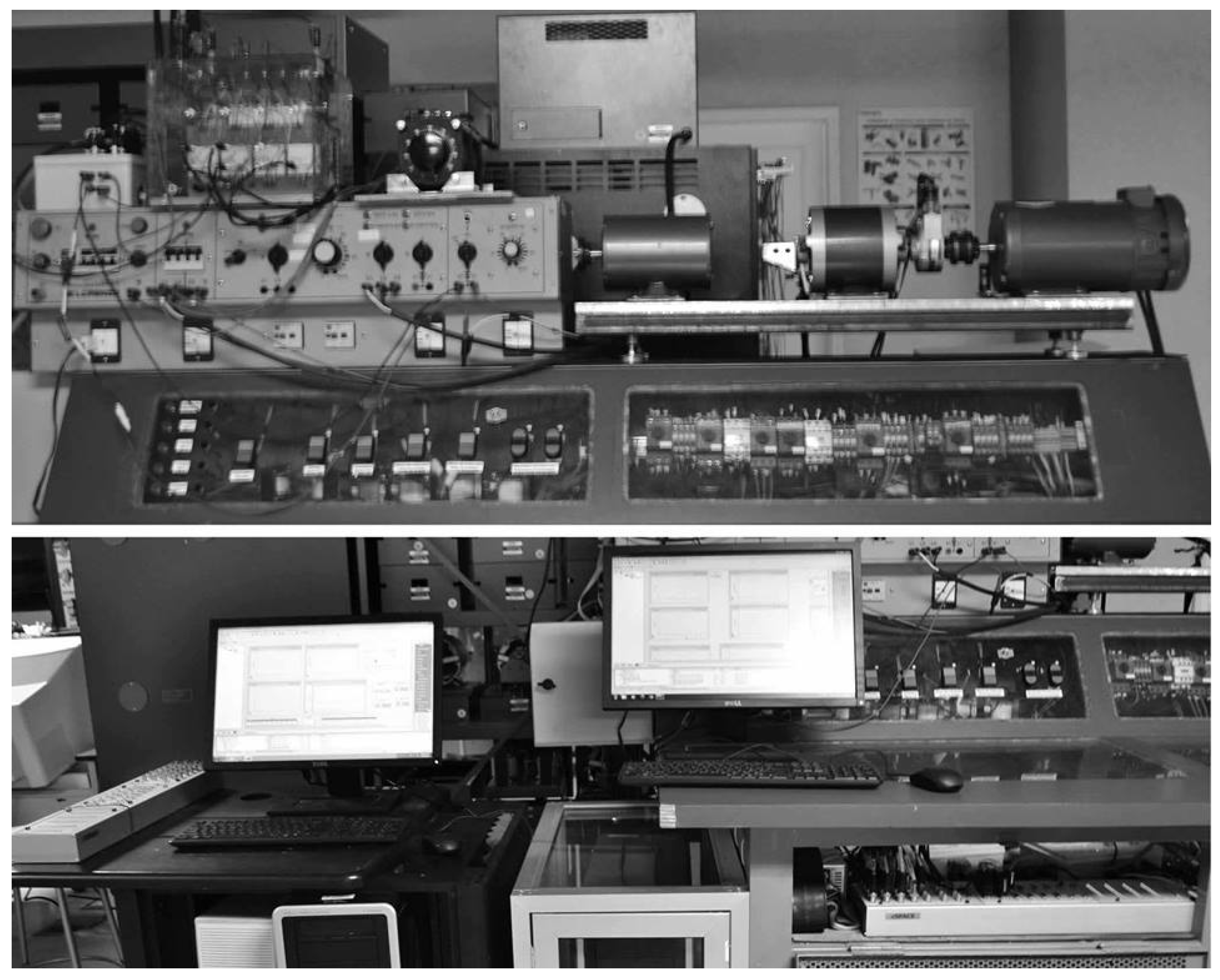
7. Experimental Results

The hardware for the DC motor velocity controller is illustrated in Figure 2, and described as follows:

• A D1154 Baldor compound DC motor mechanically coupled to an 8231-02 Lab-Volt squirrel-cage induction generator.
• A BEI HS35 incremental optical encoder with 2048 pulses mounted on the shaft train.
• A measurement interface with HX 05-NP current sensors to measure the field and armature currents.
• A dSPACE DS1103 data acquisition board which is linked with the real-time interface (RTI) as the display device.
• A SEMITEACH IGBT module converter by Semikron.

The nameplate data and model parameters for the DC motor are presented in

Table 1. DC motor nameplate data and model parameters.

DC Motor Nameplate Data		DC Motor Model Parameters
Power	746 W	Armature resistance $R_a$	2.18 $\mathrm{\Omega }$
Field Voltage $V_f$	115 V	Armature inductance $L_a$	13.5 mH
Armature current $I_a$	8.0 A	Series resistance $R_s$	0.28 $\mathrm{\Omega }$
Field current $I_f$	0.5 A	Series inductance $L_s$	2.7 mH
Rotor velocity ${\omega }_m$	1750 r.p.m.	Shunt field resistance $R_f$	240 $\mathrm{\Omega }$
		Shunt field inductance, $L_f$	0.642 H
		Constant motor $K_f,K_m$	1.227
		Inertia moment $J_m$	0.0026 N·m·$s^2$
		Friction coefficient $B_m$	0.0016 N·m·s
		Generator inertia moment $J_g$	0.0022 N·m·$s^2$
		Generator friction coefficient $B_g$	0.0012 N·m·s
		Turn-ratio $N_s/N_f$	0.0163

.

This paper presents results of two experiments, with a PI velocity controller and an SOSM super-twisting velocity controller, both subject to the same disturbances in the system. The first disturbance consists of applying a pulse train of the reference velocity from 1820 rpm. to 1900 rpm. with a period t = 4 s, see Figure 3a. The second disturbance is referred to the load torque applied to the DC motor when it drives a squirrel-cage induction generator above the synchronous velocity. The induction generator is characterized by delivering the generated power directly to the utility grid when it operates above the synchronous velocity and its generated power is in function of the machine slip. The tuning parameters of each controller were set experimentally to get the best dynamical velocity tracking with the square wave reference. A robust differentiator is proposed for estimating the time derivative of the velocity tracking variable; therefore, a unique speed sensor is used for both controllers. However, in order to validate the SOSM super-twisting velocity controller using the differentiator, the time derivative of the velocity tracking variable ${\epsilon }_2$ is calculated using measurements of the armature current and field current, and estimation of the load torque obtained via an asymptotic torque observer. The parameters of the asymptotic observer $l_1=1120$ and $l_2=-1285$ are defined to stabilize the observation error. For comparison purposes, the reported results of the SOSM super-twisting velocity controller using ${\epsilon }_2$ calculated are only the time-domain specifications and are included in the fourth column of

Table 2. Time-domain $PI$ and second-order sliding mode (SOSM) responses.

Time-Domain Specification	PI Controller	SOSM Controller ${\mathit{\epsilon }}_2$ Estimated	SOSM Controller ${\mathit{\epsilon }}_2$ Calculated
Rise time $t_r$ (s)	0.11	0.085	0.094
Rise settling time $t_s$ (s)	0.49	0.26	0.214
Rise overshoot $M_p$ (%)	10	6.2	3.7
Peak time $t_p$ (s)	0.22	0.17	0.17
Falling time $t_f$ (s)	0.17	0.12	0.14
Falling settling time $t_{sf}$ (s)	0.35	0.29	0.29
Falling overshoot $M_{pf}$ (%)	6.3	0	0

.

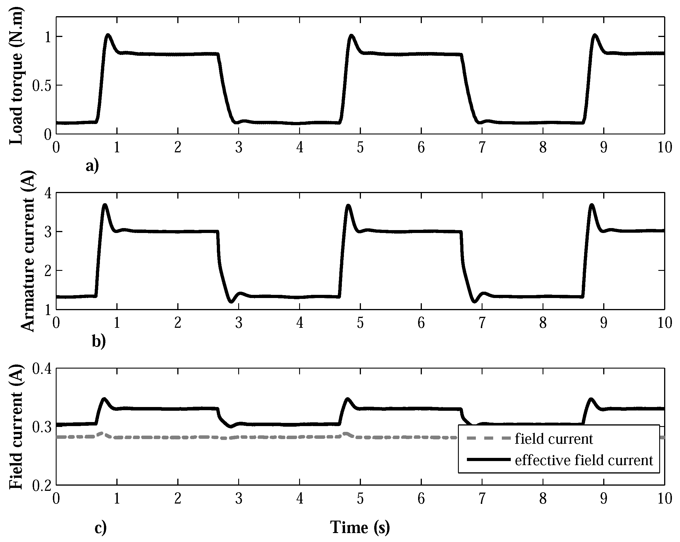
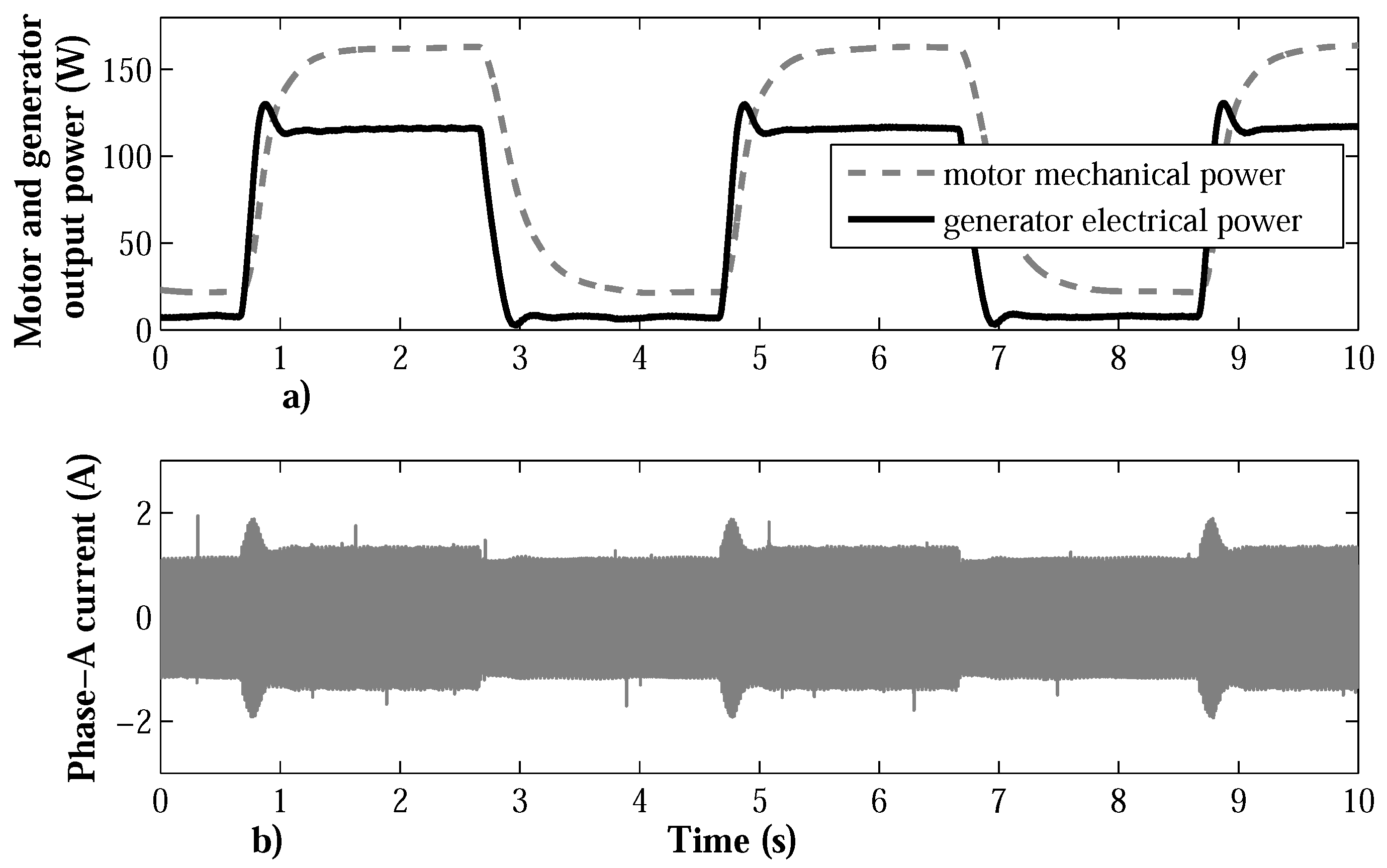
7.1. Proportional Integral Velocity Controller

The classical PI controller was tuned with the following gains: the proportional gain $K_p=5$ and integral gain $K_i=10$. These gains accomplish the inequalities (17) and (18), where $K_p>-0.34$. The velocity response ${\omega }_m$, is the controlled output variable, and achieves an acceptable velocity tracking performance, as shown in Figure 3a. The time-domain specifications for the velocity tracking, i.e., rise time, overshoot, and settling time, among others, are shown in the second column of Table 2, where the settling time is quantified into a 2% tolerance band. The control input signal $u_a$ is portrayed in Figure 3b, where it changes from 90.4 to 99.2 V, with positive peak values of 130 V. This control input corresponds to the voltage applied to armature winding and it represents the electrical input to system (1). Figure 4a shows the load torque $T_L$ which constitutes a mechanical input to a DC motor model (1) and it is modeled as external disturbance. The load torque is developed by the induction generator and it is estimated via the asymptotic observer (3), and changes from 0.12 to 0.81 N · m approximately, with an overshoot of 29%, with motor nominal torque of 1.0 N · m. The load torque response has a similar shape of the armature current $i_a$, and this current sets the electromagnetic torque, which follows the load torque according to the first state equation of DC motor model (1). The armature current $i_a$ is shown in Figure 4b, where it changes from 1.34 to 3 A, with peak values of 3.68 A, and an overshoot of 41%. When both external disturbances (changes in the velocity reference ${\omega }_{ref}$ and load torque $T_L$) are presented simultaneously in step form, the control input acts to steer the velocity error variable towards the origin and the armature current $i_a$ changes suddenly to achieve the steady state, as can be analyzed in the second equation of the DC motor model (1). Figure 4c displays the constant shunt field current $i_f$ and the effective field current $i_{eff}$, which is defined by the total effect of the magnetomotive forces of both shunt and series windings, that are connected in accumulative form (2). $i_{eff}$ varies from 0.30 to 0.33 A following armature current $i_a$ changes, and the shunt field current $i_f$ holds a constant value of 0.28 A. The mechanical power developed by the DC motor varies smoothly from 21.6 to 162 W. Simultaneously, the induction generator, as the DC motor’s load, delivers electrical power to the utility grid from 8.4 to 116.6 W, with peak values of 129.4 W when sudden changes of velocity are presented, as seen in Figure 5a. Finally, Figure 5b shows the changes of generator’s current in phase-A, which varies from a 0.78 to 0.93 A RMS, and with sudden peak values up to 1.87 A.

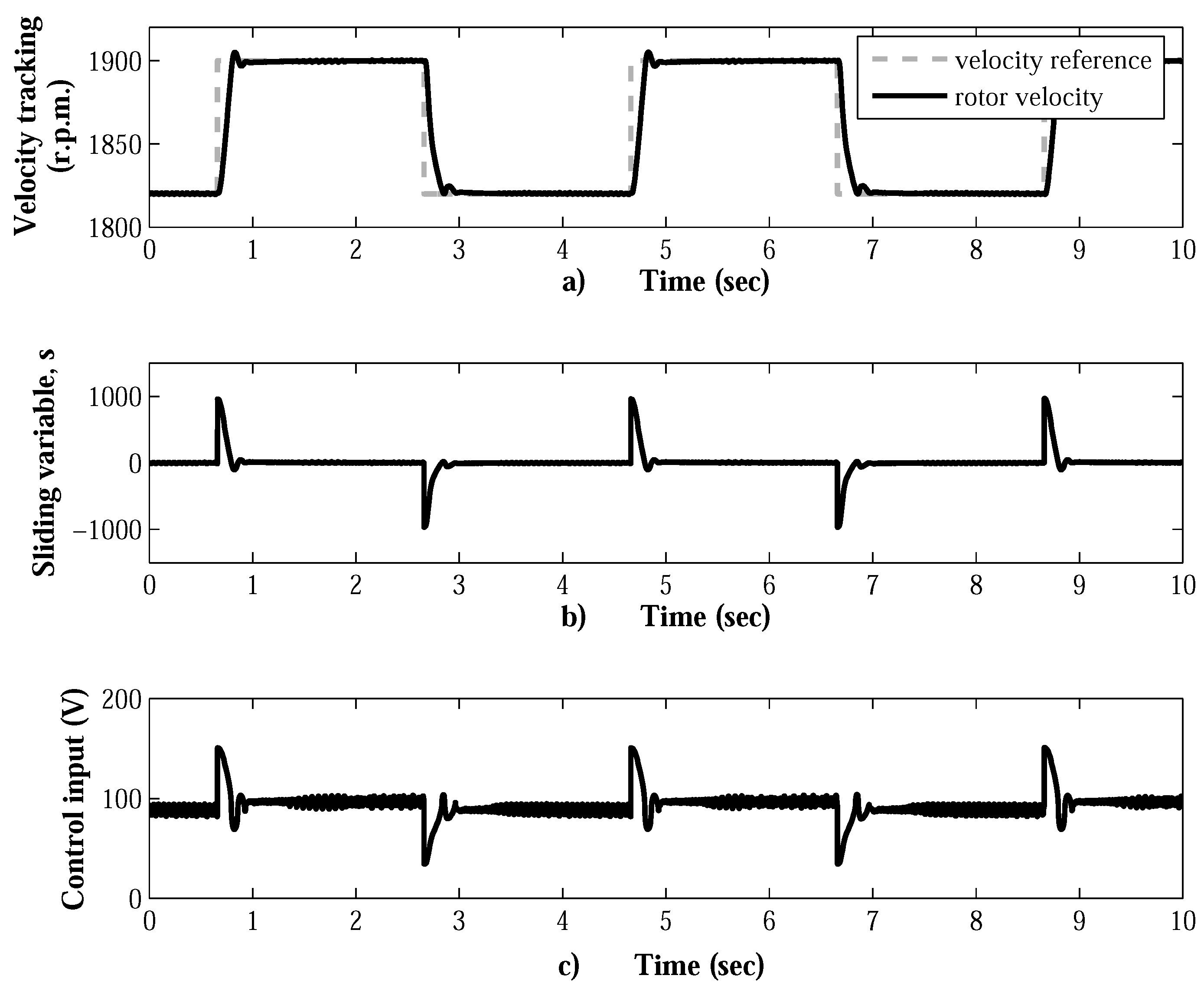
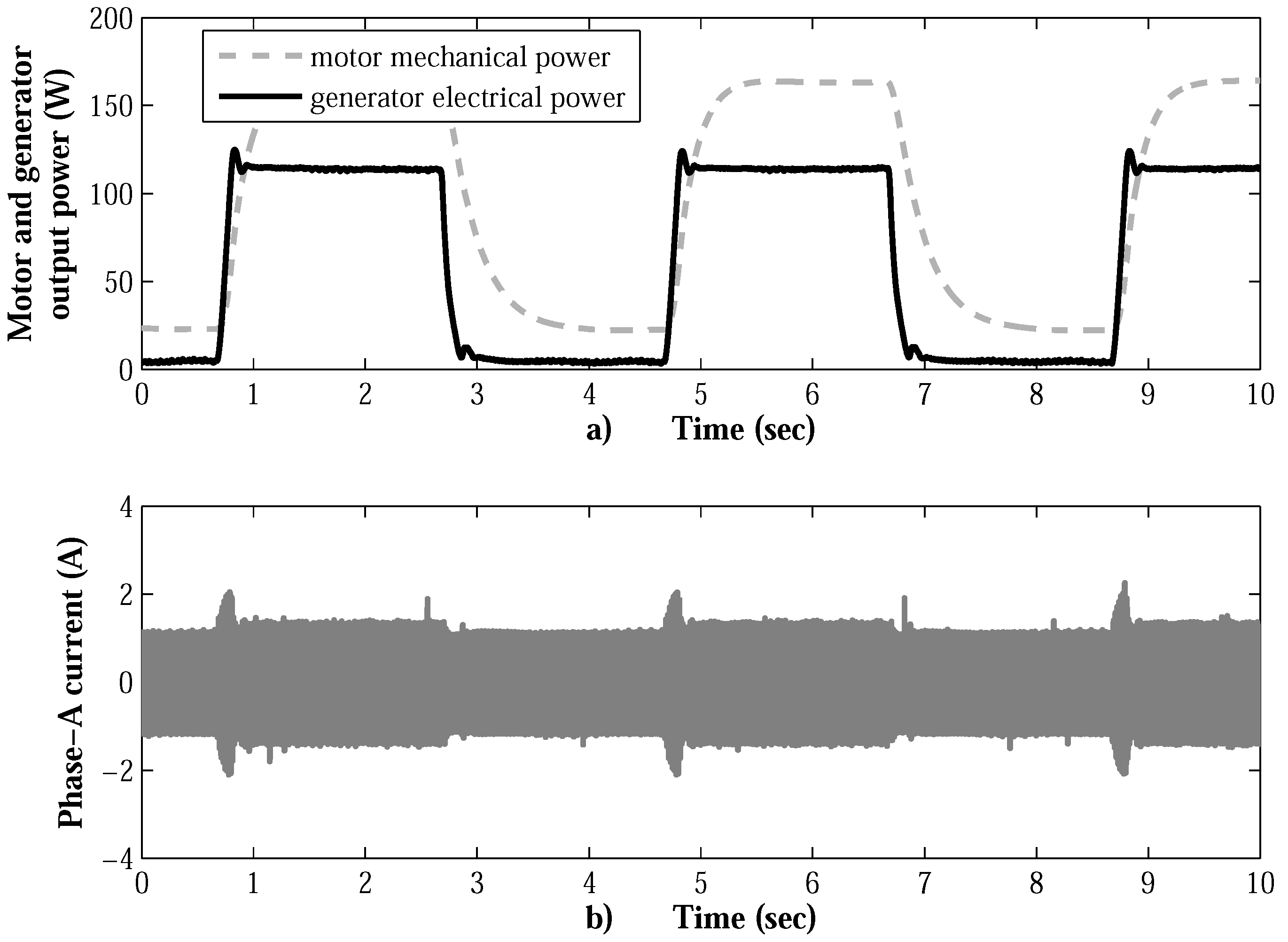
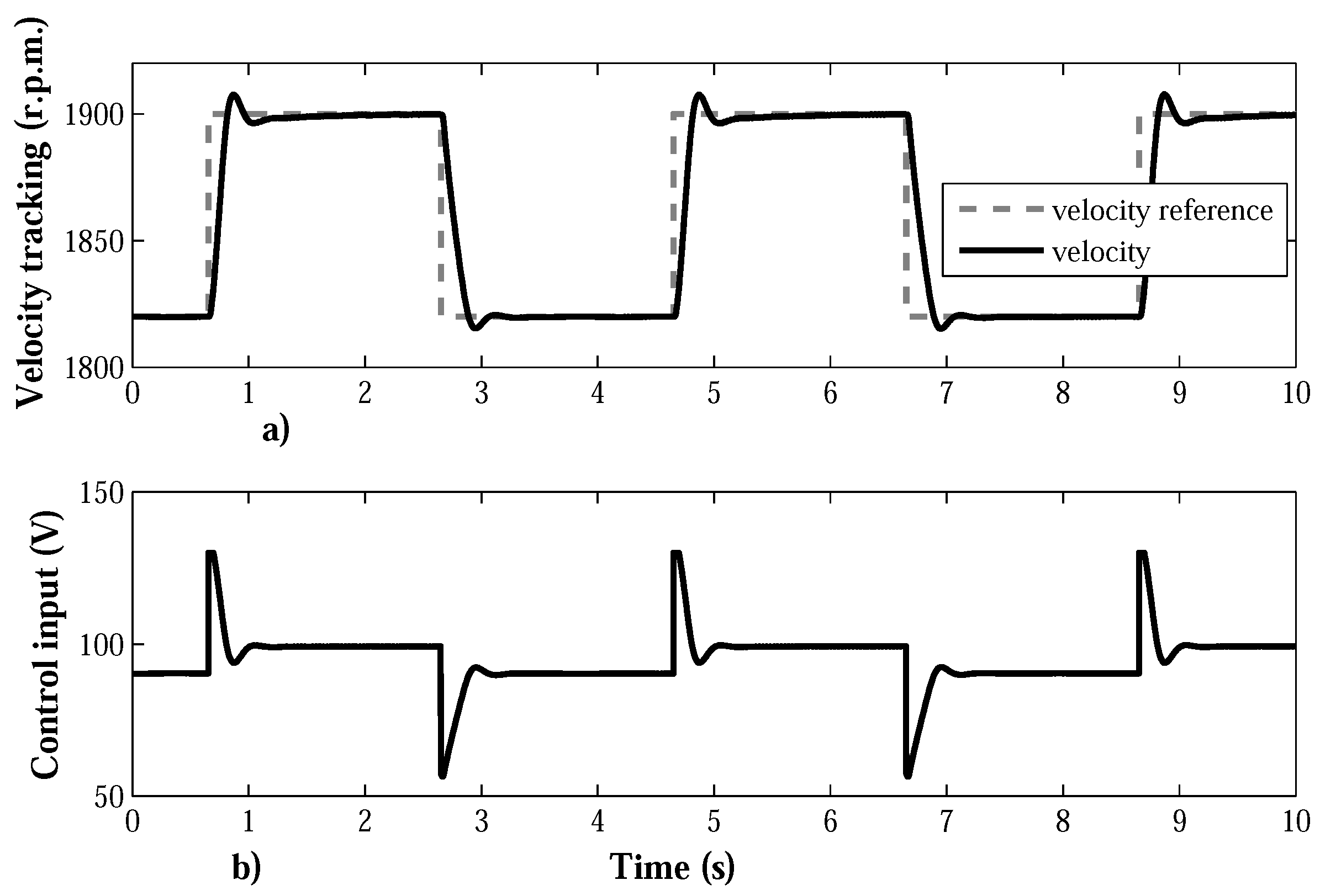
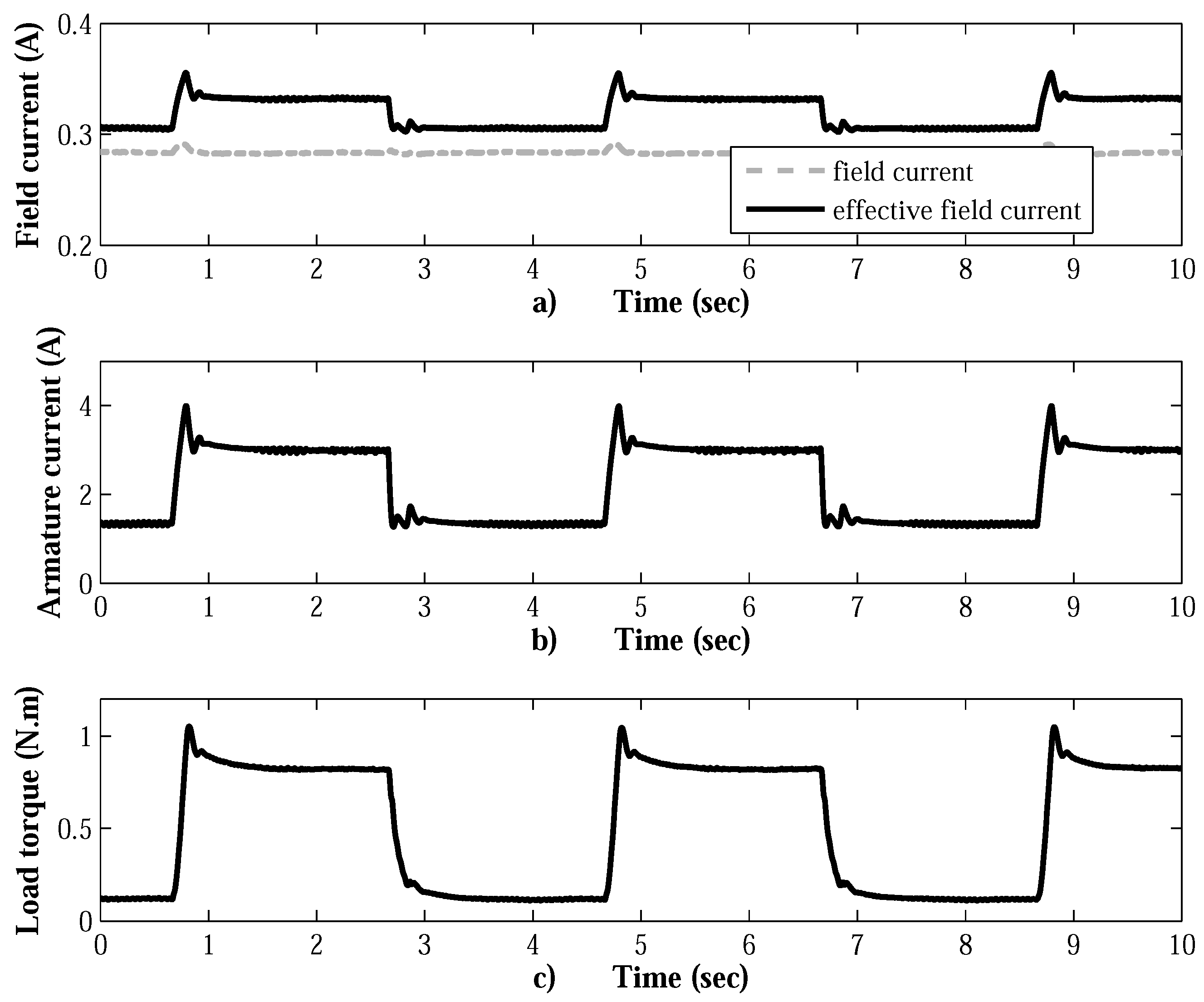
7.2. SOSM Super-Twisting Velocity Controller

The modern SOSM super-twisting velocity controller has been tuned experimentally observing the dynamic response of the tracking velocity. The used control gains are $\lambda =2$ and $\alpha =8$. In Equation (28) the disturbance modulus is defined, where the constant $\delta$ with $\delta >k_1$ (33) and $k_1=K_v\lambda =11,823$ (24). By using $\delta =1.1k_1=\mathrm{13,005}$, Equations (35) and (36) are accomplished with the assigned control gains of $\lambda$ and $\alpha$. The sliding surface, as an argument of the control law $s=C_1{\epsilon }_1+{\epsilon }_2$, is defined with the eigenvalue $C_1=100$ for the velocity tracking response with the eigenvalues of the DC motor model (1) as a reference, that are: $p_1=-30$ and $p_2=-90$. It is important to remark that the time derivative of the velocity tracking variable ${\epsilon }_2$ was estimated via a robust differentiator applying the super-twisting algorithm, which was tuned experimentally with gains of ${\lambda }_1=100$ and ${\lambda }_2=0.5$. Differentiator parameters ${\lambda }_1$ and ${\lambda }_2$ accomplish each inequality in (39) with $L=0.3$. The DC motor velocity tracking performance is shown in Figure 6a, and its time-domain specifications are shown in the third column of Table 2. From Figure 6a, it is seen that the chattering effect of the DC motor velocity is reduced and becomes imperceptible. Figure 6b shows the sliding surface s (19), where the time derivative ${\epsilon }_2$ (7) is estimated through the differentiator (39). In this Figure, the sliding surface has peak values of 950 rad/s${}^2$ when the disturbance is presented. The control input signal $u_a$ is the input of system (1) that feeds the armature winding. This input signal is illustrated in Figure 6c and has average values from 90 to 98 V and peak values of 150 V. Figure 7a shows the field current $i_f$ of the main field which is fed with constant voltage. This field current has steady values of 0.28 A, meanwhile the effective field current $i_{eff}$ varies from 0.31 to 0.33 A, due to the addition of series field magnetomotive force where the armature current flows (2). The armature current $i_a$ is displayed in Figure 7b and has average values from 1.3 to 3 A, with peak values of 4.0 A, and an overshot of 59%. When the step velocity reference changes (both in terms of rising and falling), the control input acts to steer the velocity error toward zero and the armature current rises also to achieve the steady state, as can be analyzed in the second state equation of system (1). Figure 7c depicts the load torque $T_L$ which is estimated via the asymptotic observer (3); this load torque changes from 0.1 to 0.82 Nm with peak values of 1.05 being the generator’s nominal torque of 1.0 Nm; this load torque has an overshoot of 32% on the rising edge. The load torque response has a similar shape of the armature current, as this current sets the electromagnetic torque which follows the load torque according to the first state equation of the DC motor model (1). Figure 8a shows the DCmechanical power developed by the DC motor varies continuously from 22 to 163 W. Simultaneously, the induction generator delivers electrical power to utility grid from 5 to 114 W, with peak values of 124 W; the difference in power consists of internal losses of the induction generator. Figure 8b displays the changes of the generator’s current in phase-A, which varies from 0.76 to 0.88 A RMS, with sudden peak values up to 2.0 A.

In Table 2 the results of the time-domain specifications of the closed-loop controllers presented in this work are shown. The PI controller results are in the second column, and the SOSM super-twisting controller results using differentiator are in the third column. Meanwhile, for comparison purposes in fourth column the SOSM super-twisting controller results with ${\epsilon }_2$ are calculated and shown. The results presented in this table show that both SOSM super-twisting velocity controllers have better performance than the PI velocity controller. However, the SOSM super-twisting velocity controller with a differentiator uses only a rotor velocity sensor. This characteristic represents a cheap and attractive alternative for controlling the velocity of the compound DC motor achieving better tracking performance and with the ability to reject external disturbances and parameter variations.

Figure 9 shows the performance of the robust differentiation that estimates the time derivative of the velocity tracking error. The tracking velocity error ${\epsilon }_1$ is displayed in Figure 9a with peak values of 8.3 rad/s when the reference velocity changes. By taking as visual reference the velocity error ${\epsilon }_1$, Figure 9b shows the differentiation assessment that estimates the time derivative of velocity error ${\epsilon }_2$. As can be seen, the variable ${\epsilon }_2$ estimated is around the zero value when the velocity error ${\epsilon }_1$ achieves steady state; meanwhile ${\epsilon }_2$ calculated is near of zero due to its dependency on the parameters machine, according to Equations (6) and (7).

8. Conclusions

In this work, two closed-loop schemes for controlling the velocity of a compound DC motor were developed, including practical laboratory results for their validation. The DC motor drove a wound-rotor induction generator, operated as squirrel cage which freely delivered the generated energy to the grid, when the DC motor velocity was controlled above the synchronous speed. For comparison purposes, a classical PI controller was designed as the starting point for velocity tracking of a periodic square reference signal (pulse train); then, the state-feedback linearization technique combined with the nonlinear SOSM super-twisting algorithm was applied to achieve better velocity tracking performance and to reject external disturbances. This strategy improves the performance of the closed-loop system, where the sliding variable s, as the argument of control law, was chosen using a linear combination of the velocity tracking error ${\epsilon }_1$ and its time derivative ${\epsilon }_2$. The variable ${\epsilon }_2$ was estimated by a robust differentiator using the super-twisting algorithm; in this way, the load torque estimation by an observer, the machine parameters, and the armature and field current measurements are not needed for the sliding surface definition. The experimental validation of the SOSM super-twisting velocity controller was performed through the velocity tracking of a periodic square reference signal (pulse train) above synchronous velocity, where the load torque varies according to the velocity slip of the induction generator. The time-domain specifications of the closed-loop dynamic response (overshoot, rise time and settling time) of the SOSM super-twisting velocity controller outperforms the classical PI controller. We have demonstrated that SOSM super-twisting velocity controller can be applied to the compound DC motor for emulating the wind turbine operation in a future work. Thus, the controller design process applied to wind systems can be focused on the electric generator and the converter connected to the utility grid only, even if no wind turbine is available.

References

1. Vieira, F.E.; Sales, L.; Bezerra, F. Wind Turbine Torque-Speed Feature Emulator Using a dc Motor. In Proceedings of the IEEE Power Electronics Conference, Gramado, Brazil, 27–31 October 2013. [Google Scholar]
2. Kouadria, S.; Belfedhal, S.; Meslem, Y.; Berkouk, M. Development of Real Time Wind Turbine Emulator Based on DC Motor Controlled by Hysteresis Regulator. In Proceedings of the International Renewable and Sustainable Energy Conference, Ouarzazate, Morocco, 7–9 March 2013. [Google Scholar]
3. Rhif, A. Stabilizing sliding mode control design and application for a DC motor speed control. Int. J. Inf. Technol. Control Autom. 2012, 2, 39–48. [Google Scholar] [CrossRef]
4. Castañeda, C.E.; Loukianov, A.G.; Sanchez, E.N.; Castillo-Toledo, B. Discrete-time neural sliding-mode block control for a dc motor with controlled flux. IEEE Trans. Ind. Electron. 2012, 59, 1194–1207. [Google Scholar] [CrossRef]
5. Ahmed, M.; Mazin, Z. Combined armature and field fuzzy speed control of a DC motor for efficiency enhancement. Al-Rafidain Eng. 2012, 20, 117–129. [Google Scholar]
6. Moleykutty, G.; Kartik, B.; Alan, C. Model reference controlled separately excited DC motor. Neural Comput. Appl. 2010, 19, 343–351. [Google Scholar]
7. Morfin, O.A.; Ruiz-Cruz, R.; Loukianov, A.G.; Sanchez, E.N.; Castellanos, M.I. Torque controller of a doubly-fed induction generator impelled by a DC motor for wind system applications. IET Renew. Power Gener. 2013, 8, 484–497. [Google Scholar] [CrossRef]
8. Utkin, V. On convergence time and disturbance rejection of supert-twisting control. IEEE Trans. Autom. Control 2013, 58, 2013–2017. [Google Scholar] [CrossRef]
9. Salas, O.; Castañeda, H.; DeLeon-Morales, J. Observed-based adaptive supertwisting control strategy for a 2-DOF helicopter. In Proceedings of the International Conference on Unmanned Aircraft Systems (ICUAS), Atlanta, GA, USA, 28–31 May 2013. [Google Scholar]
10. Gonzalez, T.; Moreno, J.A.; Fridman, L. Variable gain super-twisting sliding mode control. IEEE Trans. Autom. Control 2012, 57, 2100–2105. [Google Scholar] [CrossRef]
11. Evangelista, C.l.; Puleston, P.; Valenciaga, F.; Fridman, L. Lyapunov-designed super-twisting sliding mode control for wind energy conversion optimization. IEEE Trans. Ind. Electron. 2013, 60, 538–545. [Google Scholar] [CrossRef]
12. Franklin, G.; Powell, D.; Emami-Naeini, A. Feedback Control of Dynamic Systems; Prentice-Hall: Upper Saddle River, NJ, USA, 2002. [Google Scholar]
13. Utkin, V.I.; Guldner, J.; Shi, J. Sliding Mode Control in Electromechanical Systems; Taylor & Francis: London, UK, 1999. [Google Scholar]
14. Fridman, L.; Levant, A. Higher Order Sliding Modes as a Natural Phenomenon in Control Theory; Lecture Notes in Control and Information Sciences; Springer: Berlin/Heidelberg, Germany, 1995; Volume 217, pp. 107–133. [Google Scholar]
15. Chalanga, A.; Kamal, S.; Fridman, L.; Bandyopadhyay, B.; Moreno, J.A. Implementation of super-twisting control: Super-twisting and higher order sliding-mode observer-based approaches. IEEE Trans. Ind. Electron. 2016, 63, 3677–3685. [Google Scholar] [CrossRef]
16. Moreno, J.A.; Osorio, M. A Lyapunov approach to second-order sliding mode controllers and observers. In Proceedings of the 47th IEEE Conference on Decision and Control, Cancún, Mexico, 9–11 December 2008. [Google Scholar]
17. Moreno, J.A.; Osorio, M. Strict Lyapunov functions for the super-twisting algorithm. IEEE Trans. Autom. Control 2012, 57, 1035–1040. [Google Scholar] [CrossRef]
18. Derafa, L.; Benallegue, A.; Fridman, L. Super twisting control algorithm for the attitude tracking of a four rotors UAV. J. Frankl. Inst. 2012, 349, 685–699. [Google Scholar] [CrossRef]
19. Levant, A. Robust exact differentiation via sliding mode technique. Automatica 1998, 34, 379–384. [Google Scholar] [CrossRef]
Figure 1. (a) DC motor scheme, and (b) DC motor velocity controller scheme.
Energies 10 01286 g001
Figure 2. DC motor–AC induction generator group test prototype.
Energies 10 01286 g002
Figure 3. Proportional-integral ( P I ) controller. (a) Velocity tracking, and (b) control input u a .
Energies 10 01286 g003
Figure 4. P I controller monitoring signals: (a) Load torque T L , (b) armature current i a , and (c) field current i f and effective field current i e f f .
Energies 10 01286 g004
Figure 5. P I controller. (a) Motor and generator output power, and (b) phase-A current.
Energies 10 01286 g005
Figure 6. SOSM controller: (a) Velocity tracking, (b) sliding variable s, and (c) control input u a .
Energies 10 01286 g006
Figure 7. SOSM controller monitoring signals: (a) field current i f and effective field current i e f f , (b) armature current i a , and (c) load torque T L .
Energies 10 01286 g007
Figure 8. SOSM controller: (a) Motor and generator output powers, and (b) phase-A current.
Energies 10 01286 g008
Figure 9. SOSM controller: (a) velocity tracking error ε 1 , and (b) time derivative of the velocity tracking error ε 2 .
Energies 10 01286 g009