
Optimal Energy Management for Microgrids with Combined Heat and Power (CHP) Generation, Energy Storages, and Renewable Energy Sources


1
College of Information Science and Technology, Engineering Research Center of Digitized Textile and Fashion Technology, Ministry of Education, Donghua University, Shanghai 201620, China
2
Department of Automation, Shanghai Jiaotong University, Shanghai 200240, China
*
Authors to whom correspondence should be addressed.
Energies 2017, 10(9), 1288; https://doi.org/10.3390/en10091288
Submission received: 26 July 2017
/
Revised: 20 August 2017
/
Accepted: 25 August 2017
/
Published: 29 August 2017
(This article belongs to the Special Issue Distributed Energy Resources Management)
Abstract
:This paper studies an energy management problem for a typical grid-connected microgrid system that consists of renewable energy sources, Combined Heat and Power (CHP) co-generation, and energy storages to satisfy electricity and heat demand simultaneously. We formulate this problem into a stochastic non-convex optimization programming to achieve the minimum microgrid’s operating cost, which is difficult to solve due to its non-convexity and coupling feature of constraints. Existing approaches such as dynamic programming (DP) assume that all the system dynamics are known, which results in a high computational complexity and thus are not feasible in practice. The focus of this paper is on the design of a real-time energy management strategy for the optimal operation of microgrids with low computational complexity. Specifically, derived from a modified Lyapunov optimization technique, an online algorithm with random inputs (e.g., the charging/discharging of energy storage devices, power from the CHP system, the electricity from external power grid, and the renewables generation, etc.), which requires no statistic system information, is proposed. We provide an implementation of the proposed energy management algorithm and prove its optimality theoretically. Based on real-world data traces, extensive empirical evaluations are presented to verify the performance of our algorithm.
1. Introduction
Microgrids stand a good chance of becoming a future power grid paradigm that uses centralized power grids as well as local generated energy [1]. They can be operated with or without a grid connection. Microgrids usually consist of distributed renewable energy, decentralized energy storage devices (e.g., PHEVs), a local CHP System (e.g., gas-fired generators), and flexible loads.
With environmental concerns growing, a future power grid is expected to integrate more renewable energy (e.g., solar or wind) to reduce the discharge of greenhouse gas. For instance, the European Commission intends to include 20% renewables into the EU energy profile by 2020 [2], and California aims to get 33% of retail sales from renewables by 2020 [3]. As we know, the generation of renewable energy is intermittent and non-dispatchable. If we simply integrate large amounts of renewable energy, the system will encounter some reliability problems. Besides, renewable energy supply is a stochastic process, which brings a new dimension of uncertainty to energy management. Therefore, how to integrate the generation of renewables efficiently and ensure the reliability of our system simultaneously is of great importance for microgrids.
Energy storage devices are utilized to smooth energy fluctuations and reduce the system cost in a more environmentally friendly way by intelligent charging/discharging, which plays an important role in microgrids [4,5,6,7]. Apart from its power management capability, energy storage devices can act as a backup in microgrids when the external grid breaks down, which will reduce the negative effects with a quick response [8,9]. The distributed storage plays a significant role in the design and evolution of a power grid, and particularly increases additional design choices for reducing the operating cost of microgrids [10,11,12]. The hybird energy storage system is considered for primary frequency control using a dynamic droop method in an isolated microgrid power system [13]. Online energy management algorithms are developed to investigate the operating cost reduction for microgrids with an energy storage system [14].
Apart from renewables generation and energy storage devices, CHP systems are becoming very popular in the microgrids industry [15,16]. CHP systems can generate both electricity and thermal energy simultaneously, which can achieve a much higher energy efficiency than generating electricity and heat separately [17]. The characteristics of local generations and local consumptions of micrigrid make it more flexible in the utilization of renewable energy and CHP generation, which extends the adaptability of a traditional centralized grid. The power management strategy between different elements should be considered in order to design feasible control algorithms for microgrid systems [18]. Furthermore, with the augmentation of CHP generation technology, microgrids can often be much more economical than the traditional grid by using centralized grid supply and separate heat supply [19,20]. The integration analysis of hybrid energy storage system and novel CHP systems in residential scenarios are also investigated [21].
In this paper, we consider the grid connected microgrid. We aim to propose an intelligent scheduling action (e.g., charging/discharging of energy storage device, power drawn from centralized grid, power obtained from local generator, etc.) to achieve the operating minimum cost of microgrids while considering all the random inputs of the system. We first formulate the problem of achieving the minimum operating cost in microgrids as a stochastic non-convex programming. Considering that the dependence between power level of the battery pack and heat level of the water tank leads to this problem’s non-convexity, we study the relationship between them and convert it into stochastic convex optimization programming. Then we adopt the Lyapunov optimization [22] approach to design an online algorithm of some random system inputs (e.g., the charging/discharging of the energy storage devices, power from the local generator, the electricity from the power grid, and the renewable energy generation from different sources, etc.), which requires no statistic information of our system.
The contributions of this paper are summarized as follows:
- We formulate a stochastic non-convex programming for the online scheduling problem to minimize the microgrid’s cost, which captures the randomness in stochastic renewables, power and heat demands, charge level of energy storage, co-generation and physical constraints as well.
- To solve this stochastic non-convex optimization problem, we convert it into the subproblem with convex property. Then we design an online algorithm to reduce the operating cost of microgrids by using the Lyapunov optimization approach which relies on no future knowledge about the system inputs with stochastic distribution. In this way, we can get the optimal average cost.
- Through our evaluations by using practical data traces, we can see that by the proposed algorithm, we can achieve an approving empirical optimality ratio.
2. System Model and Problem Statement
The following components are typically included in our designed system: centralized power grid (supply power to the electricity load and charge the battery in an on-site way), large capacity battery (power energy storage), local co-generator (generate both heat and power energy simultaneously), external gas station (supply heat demand), thermal storage device (heat energy storage), and renewables generation (e.g., wind or solar). The system model is shown in Figure 1. For convenience of analysis, we assume that the system operates in discrete time with time slot . We then divide the time slots into frames of size T. Figure 2 gives the time structure of slots and frames. Let denote the set of time slots in time frame m, i.e., . This structure of time slot and time frame is defined to illustrate the time scales of the system operation for easy theoretical analysis. Therefore, we have two time scales in the system.
2.1. System Model
(1) Local co-generation (CHP): We assume that electricity and heat energy can be generated simultaneously by our local generator. Here we use an idealized model, we will investigate a more practical CHP model in our future work. and are the conversion efficiencies from fuel to the electricity and thermal energy, respectively. At each time slot t, the co-generator generates electricity and thermal energy, whose amounts are denoted as and , respectively. The generated electricity can be used for power supply to directly satisfy the net power demand or be charged into the battery . Similarly, the generated thermal energy can be used for direct heat supply for users’ heat demand or be charged into the thermal tank , respectively. represents the on/off decision of the generator: represents switching on and denotes switching off in frame , which is defined as the number of slots in a frame.
(2) Centralized power grid: We assume that the power grid and microgrid are connected. The power can be acquired from the centralized power grid in an on-demand manner to meet electricity demands. The system obtains power in the amount of for satisfying demands directly and the power in the amount of for charging the battery, respectively. are defined as the upper bound of direct power supply from external power grid and denotes the upper bound of charging power for the battery from the external power grid, respectively. Then we have and , . Supposing that the power demand can be satisfied by power grid alone, we assume that holds at any time slot, where is the upper bound of .
(3) External gas station: The heat energy from the external gas station, , can be used for direct heat supply and energy charging of the thermal tank. Using to denote the fraction for charging, we denote the amount for heat supply and heat charging as and , respectively. Under the online control algorithm that we will propose later, the heat demand can be satisfied with the energy from the co-generation and gas station while the total cost can be minimized in an intelligent way which schedules the energy properly.
(4) Renewable energy: Let denote the renewable energy harvested at time t. In our model, the renewable energy is used as electricity supply for users first because it is free. If we have excess renewable energy when the power demand has been satisfied, we use this part of energy, which is called to charge into the battery. In addition, the amount of renewable energy harvested in a time slot is bounded, and thus we have . The excess renewable power that is charged to the battery cannot exceed the total amount of harvested renewable energy. Therefore, we have , where . Note that, although the system model we consider in this paper only involves the electricity renewable energy, heat renewable energy is applicable as well.
(5) Power and heat demands: In our microgrid system, the total demand includes the demand for power and heat. represents power demand at time slot t, which must be satisfied once requested. The net power demand , which is the excess of power demand over renewable energy at time slot t, equals the subtraction of power demand and renewable energy, and can be expressed as . Let denote the maximum net power demand in a time slot, then we have . The power can be acquired from power grid, local co-generator as well as the battery, denoted as , and respectively, to balance . It can be presented as follows:
Similarly, the heat can be acquired from external natural gas station, co-generation as well as the thermal tank, denoted as , and (more details about can be found in the thermal tank model) respectively, to balance the heat demand. Thus, at every time slot, we have:
Let denote the maximum heat demand in a time slot. An additional constraint has to be added to assure the balance of heat demand and supply at any time slot, where is the maximum heat output of the external gas station. Here are defined as the conversion efficiencies from gas to the thermal energy. Let parameter denote the fraction of co-generated power that is used for charging. Then denotes the fraction of co-generated power that is used for direct power supply. is defined as the dispatch ratio from CHP to thermal tank, denotes the dispatch ratio from thermal source to thermal tank. It should be noted that any stochastic information of the net power demands and heat demands is not required in our proposed algorithm. Here we use “≤” instead of “=” to insure mathematical rigorous. Actually, it could be “=” for both Equations (1) and (2) in our optimization problem. However, in the operation of the optimization problem, it should be consider the feasibility of the mathematical solution. In the algorithm design point of view, there is no difference for “=” and “≤” for Equation (2). We pointed out that if we change “≤” to “=” in Equation (2), the solution is the same. In fact, we can also change Equation (1) into “≤” and Equation (2) into “=” in the problem formulation. It has equivalent solutions for the two optimization problem.
2.2. Battery Model and Thermal Tank Model
(1) Battery model: The dynamics of battery’s state of charge (SOC) level is given as follows:
where stands for discharging efficiency of battery and denotes the charging efficiency of it. We can find that the battery must satisfy constraints of capacity and charge/discharge in any slot t.
where is the capacity of the battery and is the maximum discharging power of the battery in each time slot and is the maximum charging power of the battery in each frame.
(2) Thermal tank model: We utilize a thermal tank to store the excess heat for later use. With the charging and discharging of tank at each time slot, the heat state evolves over time:
where is the thermal tank’s heat energy state at time slot t. Because heat energy stored in the thermal tank can not exceed the capacity of thermal tank, we have:
Similarly, is the upper bound of the thermal tank and represents the discharging rate constraint of the thermal tank.
2.3. Problem Statement
System State and Constraint: According to the components described in our system, we define the system state as a state vector :
We assume that is an i.i.d. process over time. Although some of the elements in can be arbitrarily correlated, the control decisions at each time slot only depends on current system state without any future system information.
Through jointly scheduling the power and heat energy storage, centralized power grid, the renewables, and co-generation, our system can realize the goal of minimizing the long-term time-averaged operating cost. In particular, the control vector at time slot t isdefined by:
The total cost of our system includes the cost of power acquired from external power grid, the fuel consumption of the co-generation, and natural gas for generating heat, switching and sunk cost:
We denote the real-time electricity price of power grid as , which is bounded by and . and is the minimum and maximum electricity price. So we have . It should be noticed that although can also be a stochastic process, the statistics will not be depended in our algorithm. In this paper, we set the fuel price and the price of natural gas to be constants at each time slot. Actually, our algorithm is also available in the case that the fuel price and natural gas price are not fixed since our algorithm is based on the current system state which can be known at each time slot.
So far we can formulate our first optimization problem as follows:
At the beginning of each frame, the local generator make a decision on choosing the on/off statement by solving a mixed-integer stochastic optimization program with constraints. We then jointly decide other components (, , , , , , , ) in each time slot.
Solving is challenging. In this paper, we aim to develop an online algorithm which requires no system statistics and is easy to implement.
3. The Co-Generation System Scheduling Algorithm
From the above, we know that is a challenge to solve by the current algorithm due to the non-convex optimization. However, we have found a feasible method to work out a convex optimization problem already. Therefore, in this section, we will change into a convex optimization problem. It is a real-time algorithm derived from the two-timescale Lyapunov optimization techniques [23].
3.1. Problem Relaxation
Stochastic optimization framework guarantees the balance of average energy consumption and average energy generation in the long term; however, it can not provide their hard bounds in any time slot. Thus, the problem above cannot be settled directly through stochastic optimization framework under those circumstances (17). To solve the problem, we try to take expectation on both sides of (15) and (16), which leads to P2 as follows:
After those operations, we finally obtain , which fits the stochastic optimization framework. extends the limitation of Battery and Thermal tank storage. It no longer restricts the value of and in each time slot instead of restricting them in the whole process. Under the condition that the solutions must satisfy constraint (17) at each time slot, the framework is feasible to . As long as we define these two constants suitably, solutions to can also be feasible solutions to .
3.2. Online Algorithm
To simplify the following discussion, the virtual queues and are respectively defined for the battery and thermal tank as follows:
where and are two perturbation parameters, which are time-independent constants and will be specified later.
Then the queueing dynamics (15) and (16) can be transformed into:
In addition, the Lyapunov function is defined to be: . Then the T-slot conditional Lyapunov drift can be defined as follows:
Consider any , squaring both sides of (28) and (29). Considering the result in one time slot after carrying out sub calculations, we can obtain:
In each time slot, the CHP consume the fuel while the thermal source consumes the gas. The maximum amount of them are and separately. Similarly, and denote the maximum charging power from the renewable energy resource and the external power grid, respectively. We define B as: .
Summing (31) over and taking the expectation conditional on and yields:
For the purpose of keeping and stable under the stochastic optimization framework, we should minimize the right-hand side of (32). Beyond that, the goal of our control algorithm is to minimize the system energy cost. Accordingly, we set parameter V to denote the tradeoff between energy storage and consumption and the drift-plus-penalty function is defined as follows:
Replacing in (33) use . In order to facilitate the algorithm, we conduct some manipulation and get the formula:
The main concept of our control algorithm is minimizing the right-hand side of (34). In other words, by observing the system inputs, i.e., , , , and at each time slot in a frame, then the values of , , , , , , can be determined.
Derived from the analysis above, an online algorithm can be developed by solving P3:
Observing P3, we can find the problem function includes the term and with and in and in . It follows that the Hessian matrix of the function is not positive semi-definite, which makes a non-convex optimization problem and challenging to solve. However, with a further investigation of , and can be decoupled from and .
At first, we take the terms and into account. If , it is clear that ; otherwise, it can be easily obtained that . Similarly, if , we have ; otherwise, . Consequently, we can only concentrate on the key part of (36) which is listed as follows:
We discuss the solutions to minimize P3 when the local generator is on or off, respectively. We discuss the question under the circumstance that first.
First, we assume that both (37) and (40) are inactive. Analyzing those equations we can easily see the linear relationship between and . Therefore, we can set to be 0 or 1 to minimize . Similarly, and can also be decided to be 0 or 1 in order to minimize .
Secondly, supposing (37) to be active while (40) to be inactive, we have:
Replacing using (49) in (48), now the problem change into:
Then the minimum of the above equation can be achieved by setting to be 0 or 1.
Thirdly, supposing (37) to be inactive while (40) to be active, we have:
and we replace using (51) in (48), then we have:
Since , we can set both and to 1 to minimize (52).
Finally, supposing (37) and (40) to be active, we can transform the problem into:
Since , to minimize (53) we can set .
Then we discuss the circumstance that .
Because is related to , so when , . The problem is reduced to the equation as follows:
Replacing use (37). Setting or 1 can get the minimum value of . So the equation is more concise:
From this, what we need to discuss is the value of . If , to minimize (55), should be set to 0; If , we have .
The above analysis display the minimization is four different circumstances.
4. Performance Analysis
Theorem 1.
Define θ and ε to be:
Then concluding from the process of minimizing P3 we can obtain the result:
Proof.
Using induction method, the upper and lower bounds of and can be proved under (56) and (57).
- (1)
- Firstly, we show the upper bounds. The main idea is to prove that the battery and thermal tank will not charging when there level exceed and , respectively.
- Suppose . Since the electricity charged in a time slot will not be more than . Then holds, obviously.
- Suppose , i.e., . From (42), (44) and (47), it can be obtained that , , and . According to , we must set , , , to minimize the problem function, i.e., the battery will not charge when its level rises over . Accordingly, holds when . With the conclusion when , we can know that .
- Suppose . Similar to the battery, the heat charged in a time slot will not exceed . Hence, holds then.
- Suppose , i.e., . From (45) to (47), it can be obtained that , , and . According to , we must set , and to minimize the problem function, i.e., the thermal tank will not charge when its level rises over . Accordingly, holds when . With the conclusion when , we know that .
The above proof presents the upper bounds of and , i.e., the capacities of battery and thermal tank, respectively. To simplify the future investigation, we denote the capacities as and , respectively. Since the capacities are functions of V, the value of V can be changed to make a tradeoff between energy storage and cost. In contrast, the value of V can be obtained with a given battery pack or thermal tank capacity. - (2)
- Secondly, we show the lower bounds using (56) and (57). To keep and from being negative, we only need to prevent the battery and thermal tank from discharging when they can not afford, i.e., when and
- Suppose . Certainly, it follows that .
- Suppose . From (42), (47) and (56) , it can be obtained that , . According to , we have to set , i.e., the battery will not discharge. Accordingly, holds then. Consequently, we can conclude that .
- Suppose . Then follows apparently.
- Suppose . From (46) and (57), it can be obtained that .According to , we have to set , i.e., the thermal tank will not discharge. Accordingly, holds then. Finally, we can conclude that .
Theorem 1 shows that the battery and thermal tank both have finite capacities under the proposed algorithm, which means solutions of are feasible solutions to as well. ☐
Theorem 2.
The gap between the optimal cost of P1 and the expected cost obtained by solving P3 is no more than , i.e.,
where is the energy cost at time slot t under the proposed algorithm, and is the optimal solution to the original problem P1.
5. Numerical Simulations
In this section, we use Matlab to evaluate the performance of the proposed algorithms by numerical simulations. We consider a hotel with battery and thermal tank as well as the CHP system. In our simulation, each time slot represents 15 min and each frame consists of 4 time slots (i.e., one hour). The parameter settings are partly listed in Table 1 and detailed in Section 5.1.
5.1. Simulation Setup
Centralized Power Grid: We obtain the electricity price data of power grid from [24]. The data trace is shown in Figure 3. The maximal supply power and charging power obtained from power grid are both set to be 32 kWh/h.
External Gas Station: We assume that the natural gas price varies across time and has a uniform distribution between (0.004, 0.010)$/kBtu. The maximal thermal output is set as kBtu/h. The efficiency is set as .
CHP System: The maximal thermal output of CHP system is set as kBtu/h. The overall CHP efficiency is assumed to be 80%, and the electricity conversion efficiency is in the range of 30–40%. The fuel cost of CHP is set as $/kBtu. We set the minimal on/off period of CHP to be 1 h, i.e., 4 time slots. The sunk cost for maintaining the system in its active state is set as .
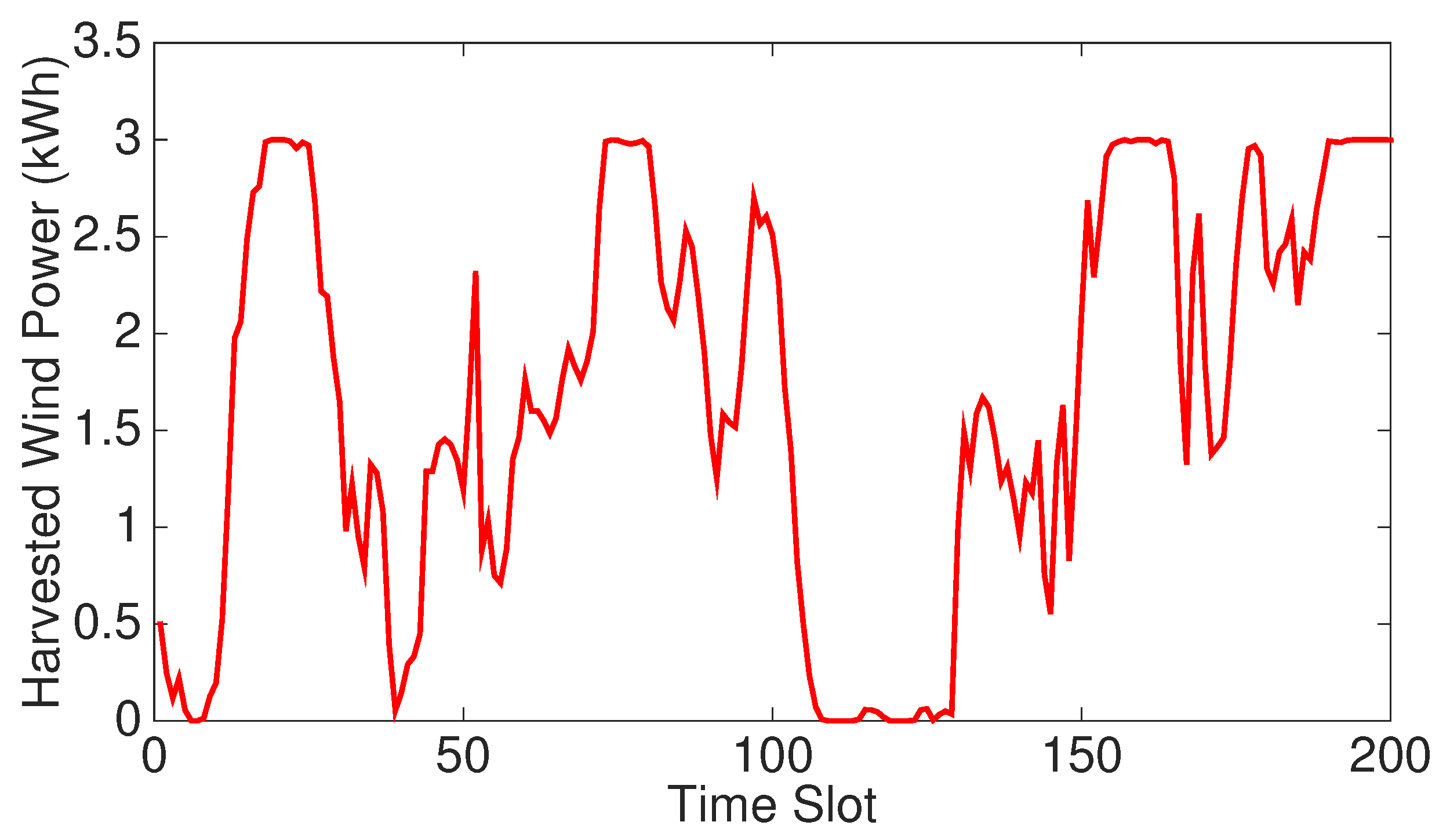
Harvested Wind Power: The harvested wind power data is obtained from [25]. The data path is shown in Figure 4.
Battery and Thermal Tank Model: We set the maximal charging and discharging rates of the battery as kWh/h and kWh/h, while the charging and discharging efficiency is set as and , respectively. Similarly, the heat storing and releasing efficiency of the thermal tank is also set as and . The maximal heat output is set as 30 kBtu/h.
5.2. Results of the Simulation
With the parameters above, we simulate for 200 time slots and each time slot stands for 15 min. We let .
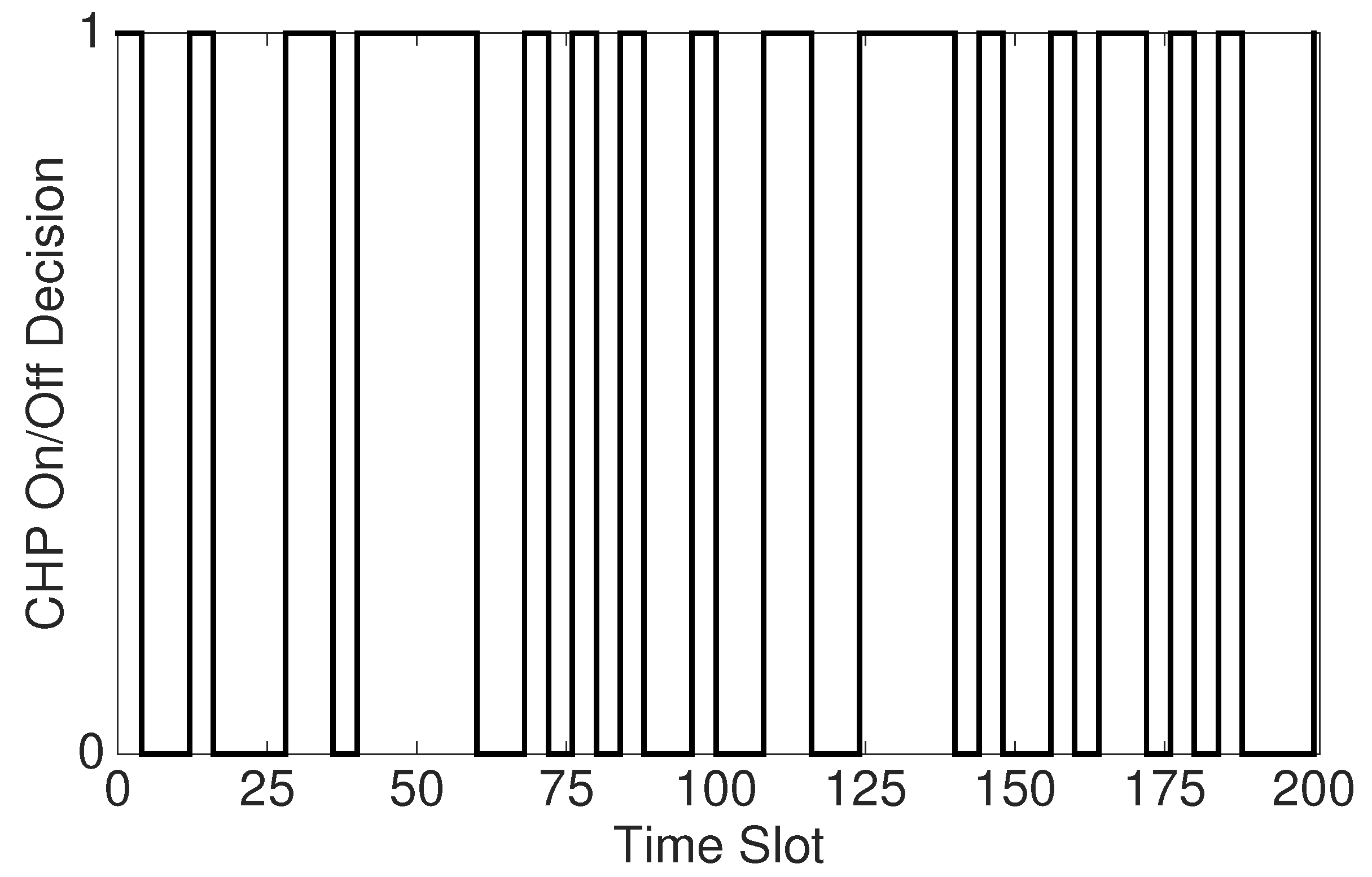
Figure 6 shows the process where the CHP system adaptively makes on/off decisions in 200 time slots. We can see that the decisions are made every 4 time slots.
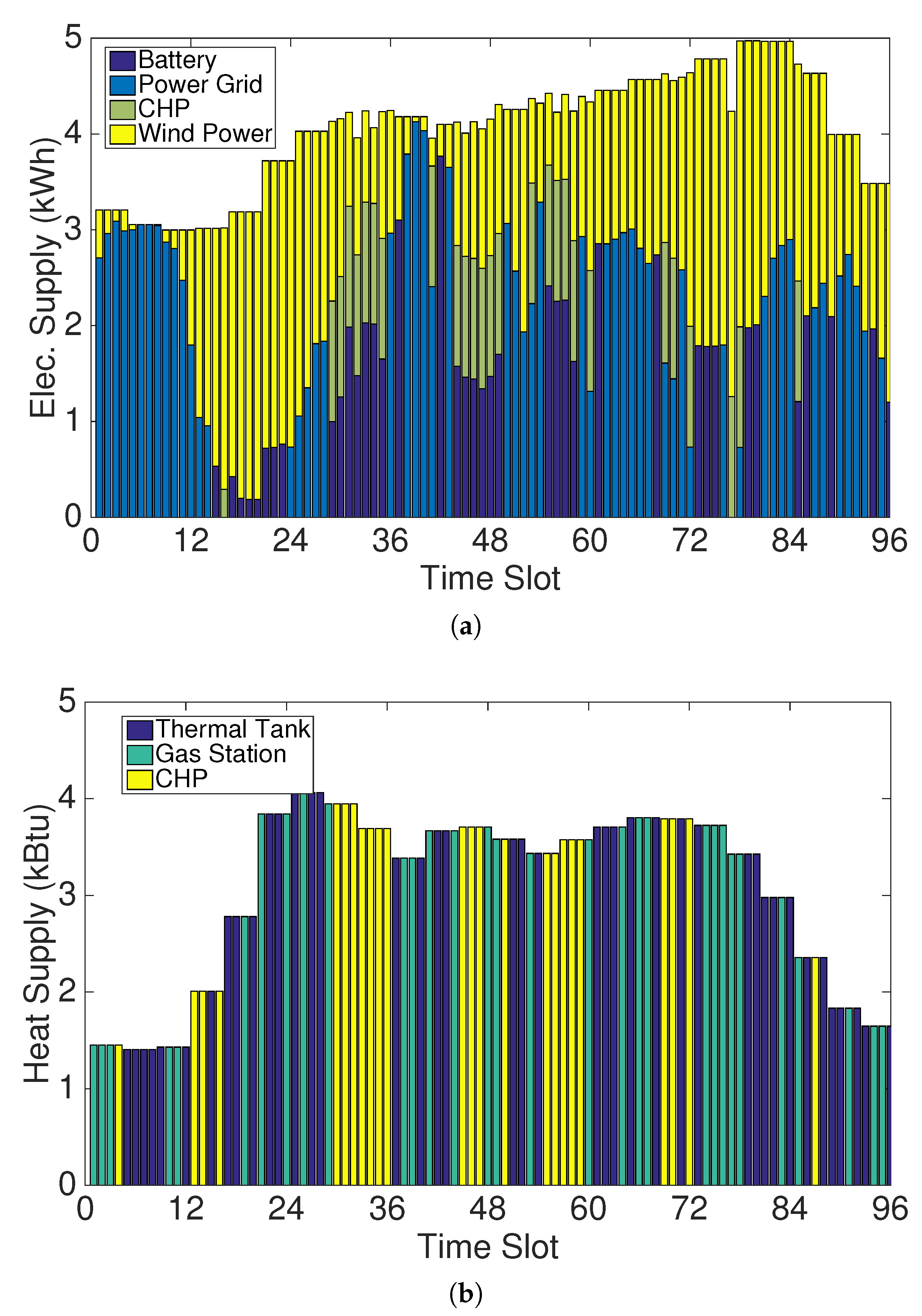
The sample paths in Figure 7 depict electricity and heat supplies in the first 24 h (i.e., 96 time slots). Both the electricity and heat demands can be satisfied with hybrid sources.
Figure 8 specifies the charging/discharging behavior of the battery and thermal tank. As shown in Figure 4 and Figure 5a, the electricity demand is larger than the harvested wind power at every time slot, there is no excessive renewable energy (wind power) left to charge into the battery. As a result, there is no wind power illustrated in Figure 7a. Actually, in our optimization problem and simulations, if there exists excessive wind power, it can be charged into the battery for future use under our designed algorithm.
Figure 9 shows the corresponding changes of battery level and thermal tank level in all the 200 time slots under . We can see that the tank level remains almost stationary due to the uniform distribution of the gas price, while the battery level fluctuates in reaction to the electricity price. However, the capacities of both battery and thermal tank are bounded.
5.3. Performance vs. V and Charging/Discharging Efficiency
With further simulations under different values of , , , and V, we observe the impacts of the weight V and efficiency of charging/discharging.
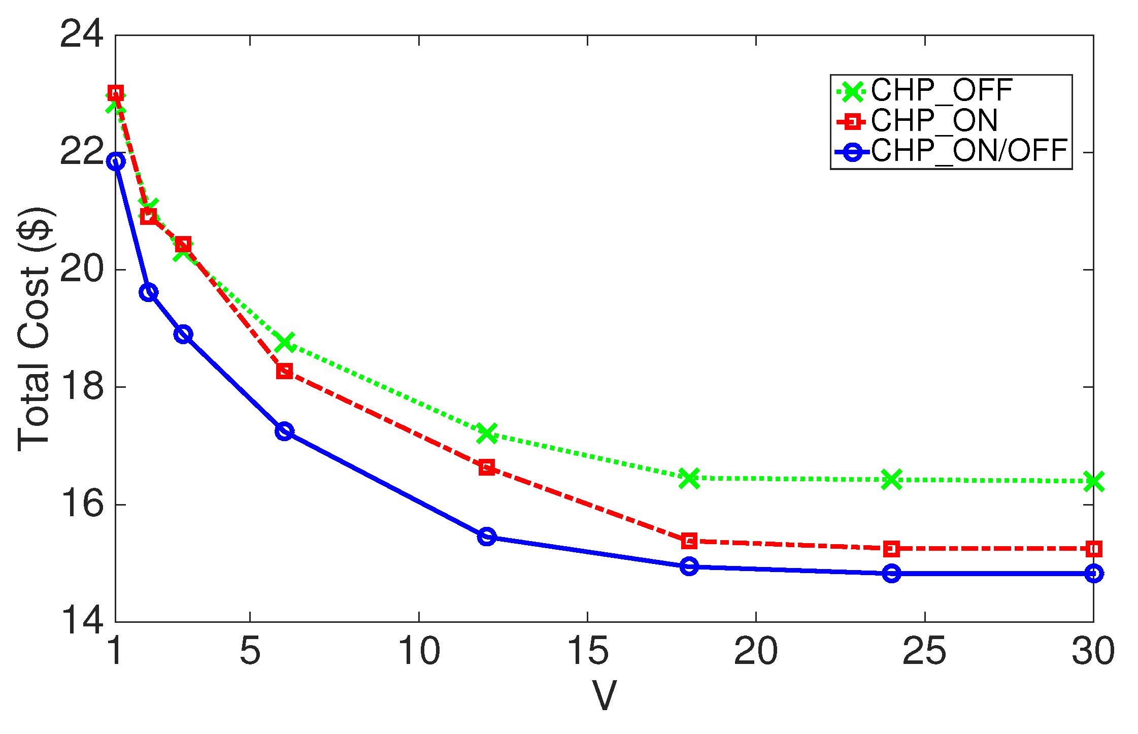
As shown in Figure 10, the cost drops when charging and discharging get more efficient. Figure 11 shows that the capacity of battery and thermal tank is linear with V, which is also indicated in Theorem 1. The total cost curve shown in Figure 12, on the other hand, converges to the minimum with increasing V. Furthermore, by comparing with the situations where CHP is permanently on and off, the effectiveness of our adaptive on/off decision policy can be verified.
6. Conclusions
In this paper, we studied the operating cost minimization problem for microgrids with CHP generation, energy storages, and renewable energy resources by using the Lyapunov approach. We designed an algorithm LYP that can achieve near-optimal performance by adjusting the value of V. According to a large amount of empirical evaluations, the microgrid operating cost can be reduced significantly through such an integration of centralized grid, renewable energy, power storage device, and co-generation.
Acknowledgments
This work is supported by the National Natural Science Foundation of China (Grant No. 61772130, 61301118); the International Science and Technology Cooperation Program of the Shanghai Science and Technology Commission (Grant No. 15220710600); the Innovation Program of the Shanghai Municipal Education Commission (Grant No. 14YZ130); and the Fundamental Research Funds for the Central Universities. This paper is an extended version of our conference paper: Optimal energy storage management for microgrids with ON/OFF co-generator: A two-time-scale approach [27].
Author Contributions
The work presented in this paper is a collaborative development by all of the authors. Guanglin Zhang and Yu Cao contributed to the idea of the incentive mechanisms and designed the algorithms. Yongheng Cao, Demin Li and Lin Wang developed and analyzed the experimental results. All authors contributed to the organization of the paper including writing and proofreading.
Conflicts of Interest
The authors declare no conflict of interest.
References
- Marnay, C.; Firestone, R. Microgrids: An emerging paradigm for meeting building electricity and heat requirements efficiently and with appropriate energy quality. In European Council for an Energy Efficient Economy Summer Study; Lawrence Berkeley National Laboratory: Berkeley, CA, USA, 2007. [Google Scholar]
- European Commission. 2020 Climate and Energy Package. 2017. Available online: https://ec.europa.eu/clima/policies/strategies/2020_en (accessed on 21 May 2017).
- Senator Energy, Utilities and Communications Committee. Senate Bill X 1-2. 2011. Available online: http://www.leginfo.ca.gov/pub/11-12/bill/sen/sb_0001-0050/sbx1_2_cfa_20110214_141136_sen_comm.html (accessed on 21 May 2017).
- Bitar, E.; Rajagopal, R.; Khargonekar, P.; Poolla, K. The role of co-located storage for wind power producers in conventional electricity markets. In Proceedings of the American Control Conference, San Francisco, CA, USA, 29 June–1 July 2011. [Google Scholar]
- Varaiya, P.P.; Wu, F.F.; Bialek, J.W. Smart operation of smart grid: Risk-limiting dispatch. IEEE Proc. 2011, 99, 40–57. [Google Scholar] [CrossRef]
- Stadler, M.; Aki, H.; Lai, R.; Marnay, C.; Siddiqui, A. Distributed Energy Resources On-Site Optimization for Commercial Buildings with Electric and Thermal Storage Technologies; LBNL-293E; Lawrence Berkeley National Laboratory: Pacific Grove, CA, USA, 2008. [Google Scholar]
- Guo, Y.; Gong, Y.; Fang, Y.; Khargonekar, P.P.; Geng, X. Energy and Network Aware Workload Management for Sustainable Data Centers with Thermal Storage. IEEE Trans. Parallel Distrib. Syst. 2014, 25, 2030–2042. [Google Scholar] [CrossRef]
- Koutsopoulos, I.; Hatzi, V.; Tassiulas, L. Optimal Energy Storage Control Policies for the Smart Power Grid. In Proceedings of the 2011 IEEE Third International Conference on Smart Grid Communications (SmartGridComm), Brussels, Belgium, 17–20 October 2011. [Google Scholar]
- Van de ven, P.; Hegde, N.; Massoulie, L.; Salonidis, T. Optimal Control of Residential Energy Storage Under Price Fluctuations. In Proceedings of the 1st International Conference on Smart Grids, Green Communications and IT Energy-Aware Technologies 2011 (ENERGY 2011), Venice, Italy, 22–27 May 2011. [Google Scholar]
- Urgaonkar, R.; Urgaonkar, B.; Neely, M.J.; Sivasubramaniam, A. Optimal Power Cost Management Using Stored Energy in Data Centers. In Proceedings of the ACM SIGMETRICS International Conference on Measurement and Modeling of Computer Systems, San Jose, CA, USA, 7–11 June 2011. [Google Scholar]
- Guo, Y.; Ding, Z.; Fang, Y.; Wu, D. Cutting Down Electricity Cost in Internet Data Centers by Using Energy Storage. In Proceedings of the 2011 IEEE Global Communications Conference (GLOBECOM 2011), Houston, TX, USA, 5–9 December 2011. [Google Scholar]
- Mishra, A.; Irwin, D.; Shenoy, P.; Kurose, J.; Zhu, T. SmartCharge: Cutting the Electricity Bill in Smart Homes with Energy Storage. In Proceedings of the 3rd International Conference on Energy-Efficient Computing and Networking (e-Energy), Madrid, Spain, 9–11 May 2012. [Google Scholar]
- Li, J.; Xiong, R.; Yang, Q.; Liang, F.; Zhang, M.; Yuan, W. Design/test of a hybrid energy storage system for primary frequency control using a dynamic droop method in an isolated microgrid power system. Appl. Energy 2017, 201, 257–269. [Google Scholar] [CrossRef]
- Chau, C.; Zhang, G.; Chen, M. Cost Minimizing Online Algorithms for Energy Storage Management with Worst-Case Guarantee. IEEE Trans. Smart Grid 2016, 7, 2691–2702. [Google Scholar] [CrossRef]
- Lu, L.; Tu, J.; Chau, C.; Chen, M.; Lin, X. Online Energy Generation Scheduling for Microgrids with Intermittent Energy Sources and Co-Generation. In Proceedings of the International Conference on Measurement and Modeling of Computer Systems (SIGMETRICS ’13), Pittsburgh, PA, USA, 17–21 June 2013. [Google Scholar]
- Zhou, K.; Cai, L.; Pan, J. Optimal Combined Heat and Power System Scheduling in Smart Grid. In Proceedings of the IEEE Conference on Computer Communications Workshops, Toronto, ON, Canada, 27 April–2 May 2014. [Google Scholar]
- ICF International Inc. CHP Policy Analysis and 2011–2030 Market Assessment; February 2012. Available online: http://www.energy.ca.gov/2012publications/CEC-200-2012-002/CEC-200-2012-002.pdf (accessed on 21 May 2017).
- Li, J.; Yang, Q.; Robinson, F.; Liang, F.; Zhang, M.; Yuan, W. Design and test of a new droop control algorithm for a SMES/battery hybrid energy storage system. Energy 2017, 118, 1110–1122. [Google Scholar] [CrossRef]
- Rooijers, F.; Amerongen, R. Static economic dispatch for cogeneration systems. IEEE Trans. Power Syst. 1994, 9, 1392–1398. [Google Scholar] [CrossRef]
- Tao, G.; Henwood, M.; van Ooijen, M. An algorithm for combined heat and power economic dispatch. IEEE Trans. Power Syst. 1996, 11, 5453360. [Google Scholar] [CrossRef]
- Li, J.; Wang, X.; Zhang, Z.; le Blond, S.; Yang, Q.; Zhang, M.; Yuan, W. Analysis of a new design of the hybrid energy storage system used in the residential m-CHP systems. Appl. Energy 2017, 187, 169–179. [Google Scholar] [CrossRef]
- Georgiadis, L.; Neely, M.J.; Tassiulas, L. Resource Allocation and Cross-Layer Control in Wireless Networks; Foundations and Trends in Networking: Hanover, MA, USA, 2006; Volume 1, pp. 1–144. [Google Scholar]
- Huang, L.; Walrand, J.; Ramchandran, K. Optimal Demand Response with Energy Storage Management. In Proceedings of the 2012 IEEE Third International Conference on Smart Grid Communications (SmartGridComm), Tainan, Taiwan, 5–8 November 2012. [Google Scholar]
- ISO New England. Available online: https://www.iso-ne.com/isoexpress/ (accessed on 21 May 2017).
- National Renewable Energy Laboratory. Available online: http://wind.nrel.gov (accessed on 21 May 2017).
- California Commercial End-Use Survey. Available online: http://capabilities.itron.com/CeusWeb (accessed on 21 May 2017).
- Shen, Y.; Ou, X.; Xu, J.; Zhang, G.; Wang, L.; Li, D. Optimal energy storage management for microgrids with on/off co-generator: A two-time-scale approach. In Proceedings of the 2015 IEEE Global Conference on Signal and Information Processing (GlobalSIP), Orlando, FL, USA, 14–16 December 2015; pp. 997–1001. [Google Scholar]
Figure 1.
Illustration of the System Model.
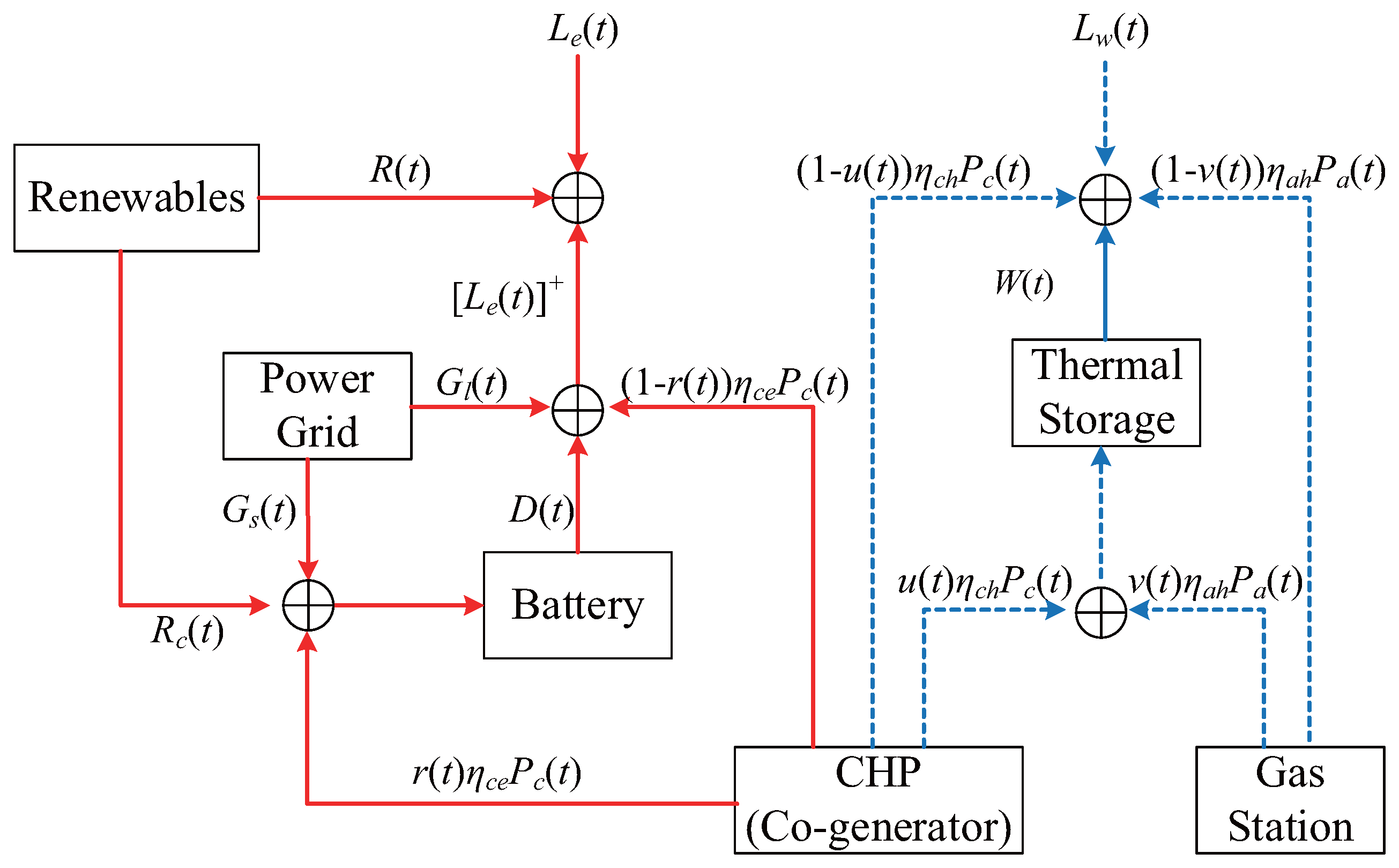
Figure 2.
Illustration of time slot and time frame.
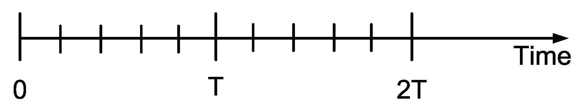
Figure 3.
Data trace of electricity market prices.
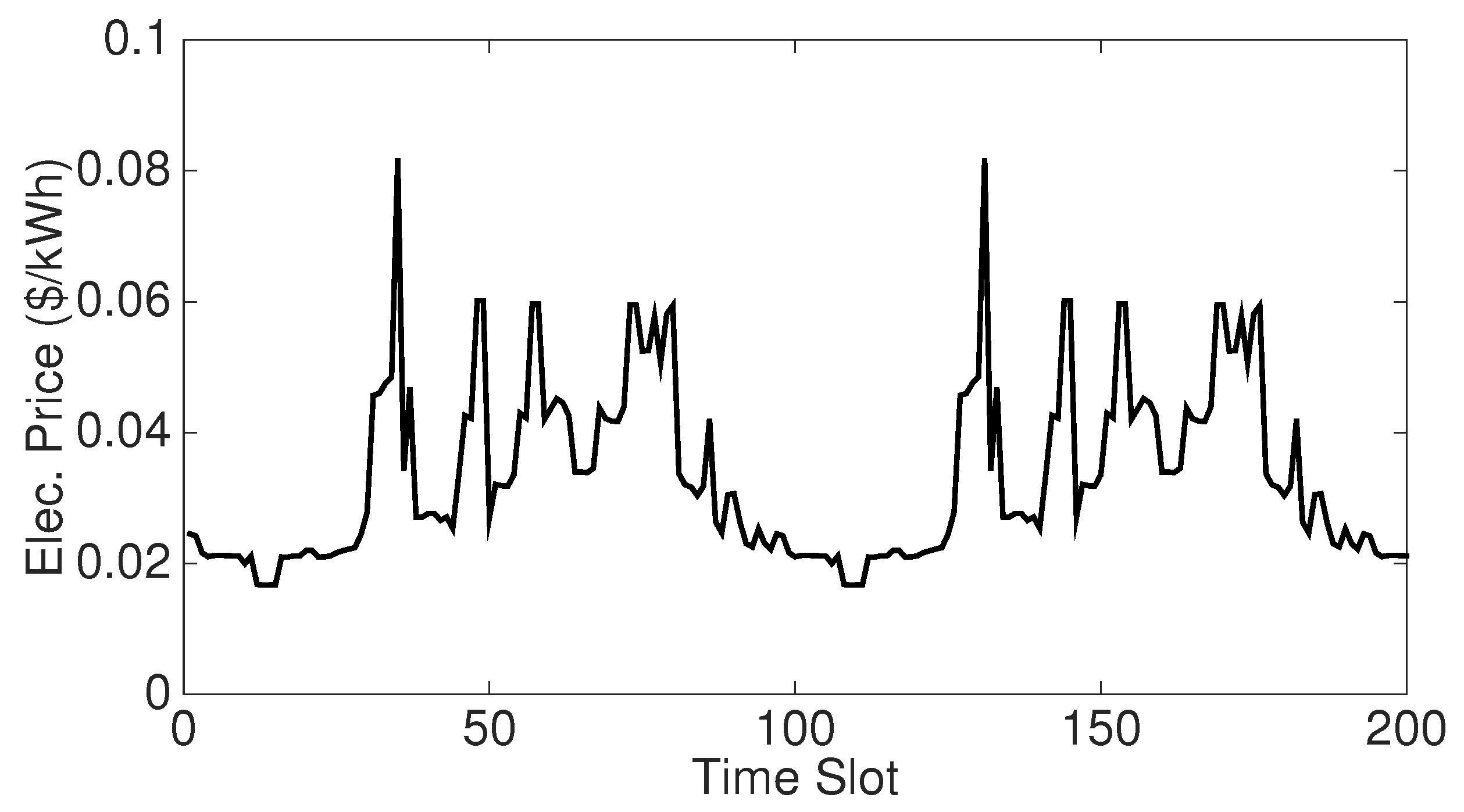
Figure 4.
Data traces of harvested wind power.

Figure 5.
Demand data traces in 50 h (i.e., 200 time slots). (a) Electricity demand; (b) Heat demand.
Figure 5.
Demand data traces in 50 h (i.e., 200 time slots). (a) Electricity demand; (b) Heat demand.

Figure 6.
A sample path of on/off decisions in 200 time slots under .

Figure 7.
Sample paths of power supplies in the first 24 h (i.e., 96 time slots) under V = 5. (a) Electricity supply; (b) Heat supply.
Figure 7.
Sample paths of power supplies in the first 24 h (i.e., 96 time slots) under V = 5. (a) Electricity supply; (b) Heat supply.

Figure 8.
Behavior of charging and discharging in the first 24 h (i.e., 96 time slots) under V = 5. (a) Amount of electricity charged(discharged) into(from) battery; (b) Amount of heat stored (released) into (from) thermal tank.
Figure 8.
Behavior of charging and discharging in the first 24 h (i.e., 96 time slots) under V = 5. (a) Amount of electricity charged(discharged) into(from) battery; (b) Amount of heat stored (released) into (from) thermal tank.
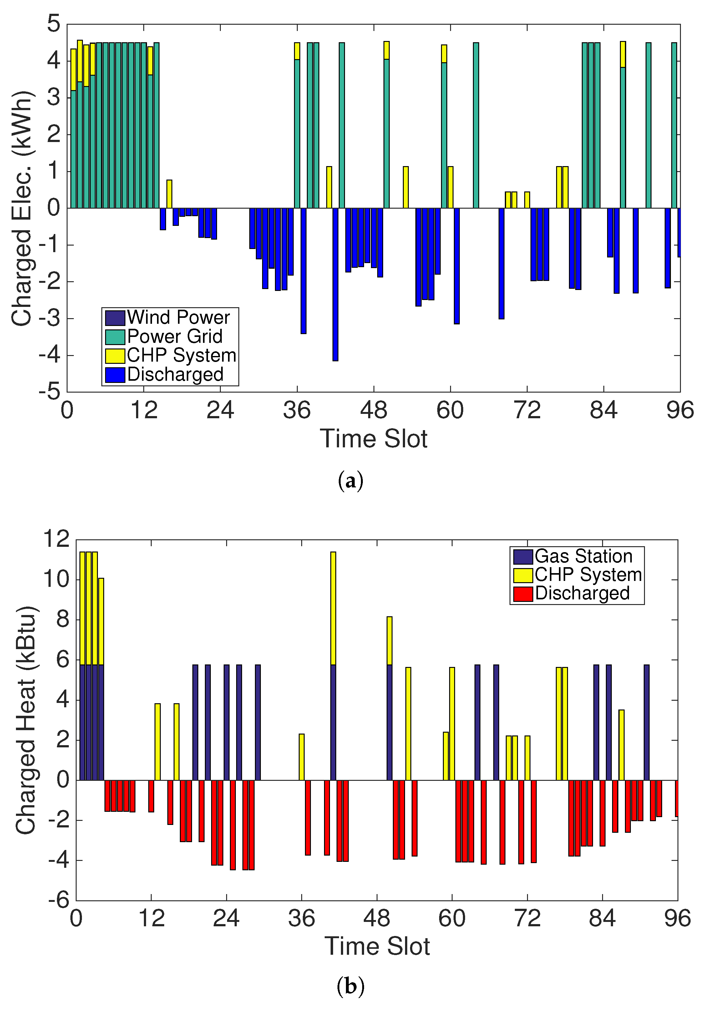
Figure 9.
Sample paths of battery level and thermal tank power level under V = 5.
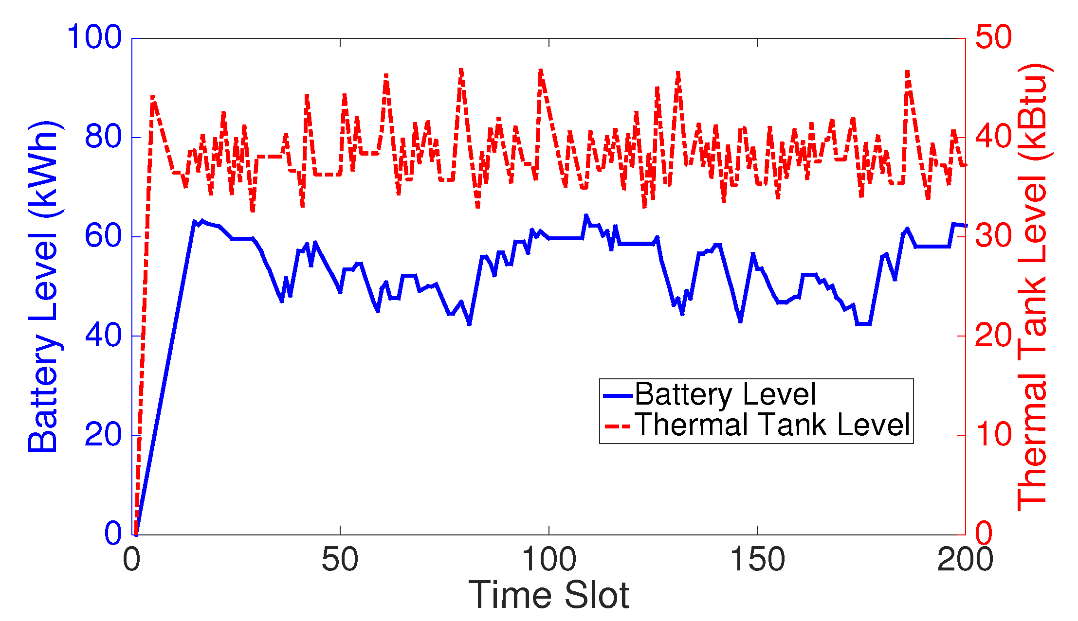
Figure 10.
Impacts of the efficiency of charging and discharging. (a) Total cost vs. and ; (b) Total cost vs. and .
Figure 10.
Impacts of the efficiency of charging and discharging. (a) Total cost vs. and ; (b) Total cost vs. and .
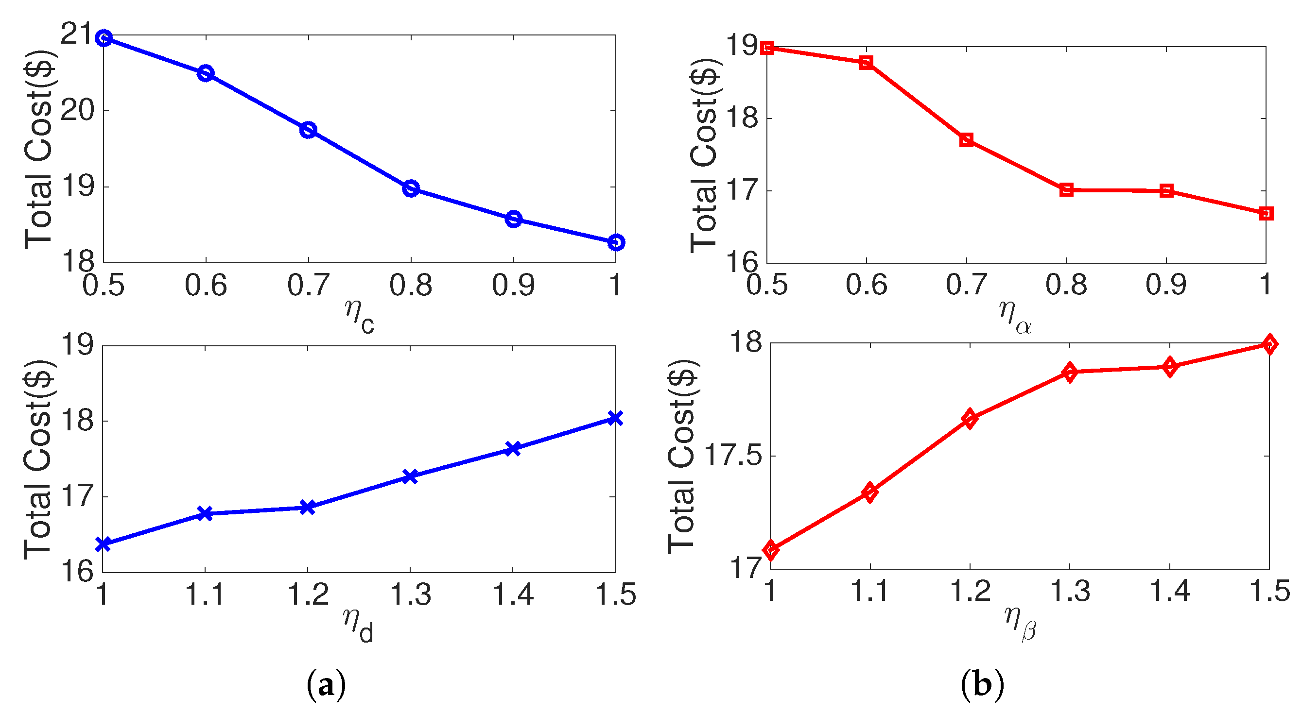
Figure 11.
Capacities of battery and thermal tank vs. V.
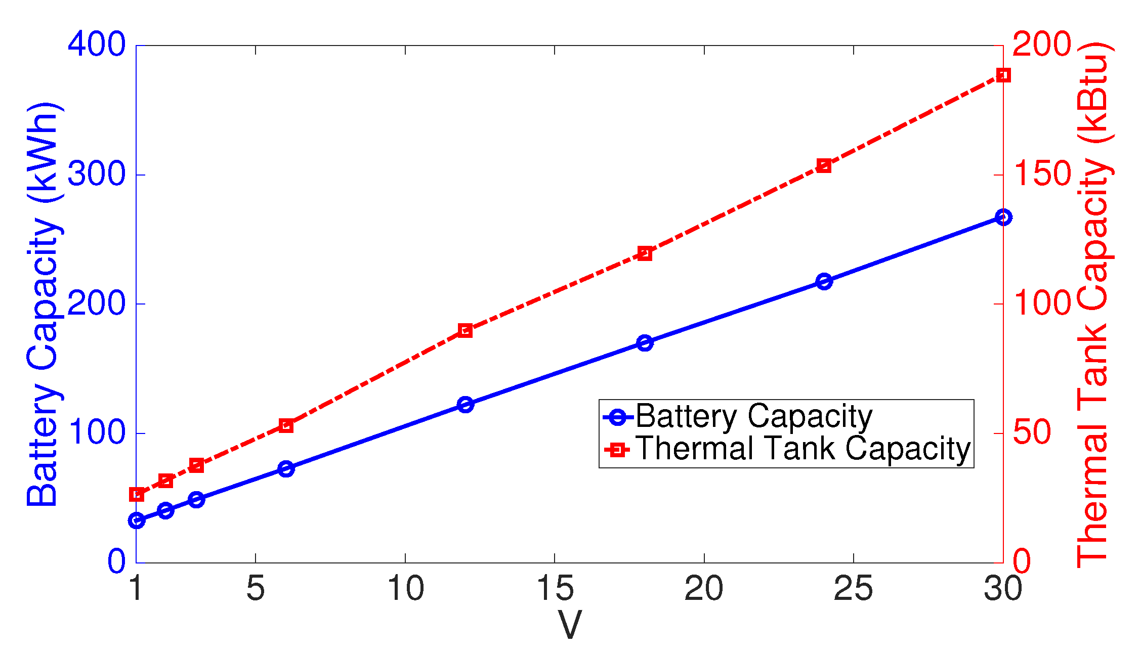
Figure 12.
Total cost vs. V under different on/off policies of CHP.


Table 1.
Parameter settings in numerical simulations.
| Parameter | Value | Unit |
|---|---|---|
| 0.8 | ||
| 0.9 | ||
| 1.1 | ||
| 0.9 | ||
| 1.1 | ||
| 0.0035 | $/kBtu | |
| 0.1 | $/h | |
| 30 | kWh/h | |
| 20 | kWh/h | |
| 32 | kWh/h | |
| 32 | kWh/h | |
| 30 | kBtu/h | |
| 50 | kBtu/h | |
| 32 | kBtu/h |
© 2017 by the authors. Licensee MDPI, Basel, Switzerland. This article is an open access article distributed under the terms and conditions of the Creative Commons Attribution (CC BY) license (http://creativecommons.org/licenses/by/4.0/).
Share and Cite
MDPI and ACS Style
Zhang, G.; Cao, Y.; Cao, Y.; Li, D.; Wang, L. Optimal Energy Management for Microgrids with Combined Heat and Power (CHP) Generation, Energy Storages, and Renewable Energy Sources. Energies 2017, 10, 1288. https://doi.org/10.3390/en10091288
AMA Style
Zhang G, Cao Y, Cao Y, Li D, Wang L. Optimal Energy Management for Microgrids with Combined Heat and Power (CHP) Generation, Energy Storages, and Renewable Energy Sources. Energies. 2017; 10(9):1288. https://doi.org/10.3390/en10091288
Chicago/Turabian StyleZhang, Guanglin, Yu Cao, Yongsheng Cao, Demin Li, and Lin Wang. 2017. "Optimal Energy Management for Microgrids with Combined Heat and Power (CHP) Generation, Energy Storages, and Renewable Energy Sources" Energies 10, no. 9: 1288. https://doi.org/10.3390/en10091288
Note that from the first issue of 2016, this journal uses article numbers instead of page numbers. See further details here.