Day-Ahead Active Power Scheduling in Active Distribution Network Considering Renewable Energy Generation Forecast Errors

College of Information and Electrical Engineering, China Agricultural University, Beijing 100083, China
*
Author to whom correspondence should be addressed.
Energies 2017, 10(9), 1291; https://doi.org/10.3390/en10091291
Submission received: 25 July 2017
/
Revised: 21 August 2017
/
Accepted: 25 August 2017
/
Published: 29 August 2017
(This article belongs to the Section F: Electrical Engineering)
Abstract
:With large-scale integration of distributed energy resources (DERs), distribution networks have turned into active distribution networks (ADNs). However, management risks and obstacles are caused by this in due to renewable energy generation (REG) forecasting errors. In this paper, a day-ahead active power scheduling method considering REG forecast errors is proposed to eliminate the risks, minimize the costs of distribution companies and achieve optimal power flow. A hierarchical coordination optimization model based on chance constrained programming is established to realize day-ahead optimal scheduling of active power in ADNs coordinated with network reconfiguration, achieving an optimal solution of network topologies and DER outputs. The hierarchical method includes three levels: the first level provides initial values, and multiple iterations between the second and third level are used to solve the multi-period mixed integer nonlinear optimization problem. The randomness due to REG forecast errors is tackled with chance constrained programming in the scheduling procedure. The hybrid particle swarm optimization algorithm is employed to solve the proposed model. Simulation results verify the validity of the proposed method with an improved 33 nodes distribution network.
1. Introduction
Recently, a large number of distributed energy resources (DERs), such as distributed generation (DG), electrical energy storage (EES), and controllable loads (CLs), are being placed in medium-voltage distribution networks for energy conservation, emissions reduction and environmental protection [1]. With these DERs, information and communication technologies (ICT) and power electronics-integrated devices have rapidly developed in the distribution networks, which thus have evolved into active distribution networks (ADNs). However, the changes bring new risks for ADNs in some respects, such as communication network security [2], operation of integrated devices [3], predictive maintenance [4] and systematic optimal operation [5]. Among these respects, for a distribution system operator (DSO), the risk of systematic optimal operation is a priority and a main task needed to be resolved.
Regarding systematic optimal operation, the main risk is the variability and limited predictability of renewable energy generations (REGs), including wind turbines (WTs) and photovoltaics (PVs), which bring uncertainties to distribution networks [6]. The difficulty of scheduling for DSO is increased due to the randomicity of REGs. On the other hand, controllable DERs, such as micro-turbines (MTs) and interruptible loads (ILs), can be used to optimize power flow. In order to eliminate the risk and take full advantage of DERs, the concept of ADN management (ADNM) has emerged to achieve a cost-effective and safe operation in ADNs [7].
ADNM includes several respects, such as active power scheduling, network reconfiguration, reactive power control and control of voltage regulation devices. In most literatures about reactive power control and control of voltage regulation devices [8,9], reactive power of DERs is controlled under a given optimal active power. Therefore, regarding day-ahead optimal scheduling problem, active power scheduling is a priority to meet the active power needs of loads and provide the optimal active power results for reactive power optimization. In an ADN, active power scheduling adjusts the outputs of controllable DERs, based on which the risks of overvoltage are eliminated and network losses are reduced [10]. Network reconfiguration is an important means to achieve an optimal operation by adjusting network topologies for ADNM, based on which loads can be balanced between lines [11]. Both network topologies and DER outputs can be optimized to improve the power flow and achieve system support in a day-ahead energy market [12]. In addition, remotely controlled switches (RCSs), which can realize network reconfiguration, should be considered in ADNM because the utilization efficiency of distribution network assets can be improved and the upgrade of distribution networks can be delayed based on the coordination between RCSs and DERs. Therefore, it is necessary to integrate distribution network reconfiguration with active management of DERs.
Network reconfiguration and DER scheduling were considered separately in the majority of literatures, and few of them realized the coordination optimization of RCSs and DERs. In [13,14], network reconfiguration was implemented in a distribution network with uncontrollable DGs. Reference [13] presented a method to solve the network reconfiguration problem in the presence of DG with an objective of minimizing real power loss and improving voltage profile in distribution system. Reference [14] considered uncontrolled DGs’ influence on distribution network reconfiguration, and a probabilistic power flow based on the point estimate method was employed to include uncertainty in WTs output. In terms of DERs operation control, taking microgrid as research object, reference [15] proposed a microgrid optimal scheduling model to minimize the microgrid total operation cost which comprises the generation cost of DERs and cost of energy purchase from the main grid. From the perspective of ADN, reference [16] set up an optimization model scheduling DERs’ outputs on day-ahead and intra-day time scales.
References [17,18,19] combined network reconfiguration and DERs scheduling to optimize day-ahead power flows, however, all of them optimized DER outputs and network topologies based on deterministic outputs of REGs, without considering high REG forecast errors [20], which may result in overvoltage risks in actual operation. Reference [17] presented a two-stage energy coordination scheduling algorithm, which showed that the coordination of flexible network topology with the continuous active management of energy resources allowed improving the efficiency of power delivery in ADN. On the basis of references [17,18] distributed energy storage was added into the energy scheduling model. An operational scheduling framework was proposed to optimally control active elements of the network and effectively utilize the hourly network reconfiguration capabilities, seeking to minimize the day-ahead total operation costs in reference [19], and the proposed model was formulated as a mixed-integer nonlinear problem and tackled with the genetic algorithm.
The day-ahead coordinated optimization of RCSs and DERs is very difficult to solve through the mentioned methods, such as optimal power flow (OPF) algorithm [17,18] and genetic algorithm [19], considering REG forecast errors. That is because the proposed problem is a complex multi-period mixed integer nonlinear optimization (MP-MINLO), in which both continuous (DERs) and discrete (RSCs) variables in 24 h are included, and solution space will increase geometrically [21]. The MP-MINLO problem is expressed in one OPF model and solved in one step including all the variables for 24 h in [17,18,19] and it is hard to find the optimal solution without effective methods to reduce the solution space. Moreover, REG forecast errors makes the proposed problem into a stochastic active power scheduling problem and the methods mentioned in [17,18,19] are hard to resolve a stochastic optimization problem.
Regarding the above questions, the original contributions of this work are as follows:
- (i)
- Day-ahead active power scheduling in ADNs coordinated with network reconfiguration considering REGs forecast errors is realized in this paper. REG outputs are described through multi-state models according to REGs’ forecast errors, and the difficulty of the modeling and solving can be reduced. The randomicity of REG outputs is solved by chance constrained programming (CCP), and optimal results satisfying a certain confidence level can be achieved, which can reduce operation risks effectively.
- (ii)
- A hierarchical coordination optimization method is proposed to solve the MP-MINLO problem with randomness, in order to achieve an optimal solution of network topologies and DER outputs. A three-level hierarchical optimal model based on CCP is established for 24 h. The first level is initial optimization, in which controllable DG outputs, shedding powers from ILs and network topologies are optimized statically in each hour. Optimization results are served as the initial values of other two levels. In the second level, the RCS states are optimized by dynamic network reconfiguration considering the limited number of RCS switching actions in 24 h, so as to avoid frequent RCS switching actions. The third level is DER optimization, in which the controllable DGs outputs and the shedding powers from ILs are adjusted according to the network topologies obtained from the second level. Then multiple iterations are needed between the second and the third level to acquire the optimal results of DER outputs and RCS states. Finally, the hybrid particle swarm optimization algorithm is employed to solve the proposed model.
The proposed multi-level method for a large number of periods divided the problem according to different physical characteristics of RCSs and DERs: RCSs are discrete variables and the maximum number of its switching actions is limited in one day on account of the wear and tear on RCSs and loop current when switching, while DERs are continuous variables and their outputs can be adjusted frequently in each hour. Initial optimization can improve searching efficiency and narrow the solution space effectively. RCSs and DERs optimizations optimize discrete and continuous variables respectively, so dimension of variables is decreased. Continuous and discrete variables are optimized separately in an efficient way.
The rest of this paper is organized as follows: Section 2 presents a calculation method for dynamic active power of REGs considering forecast errors. Section 3 addresses the proposed hierarchical coordination optimization model. The optimization algorithm for solving the model is provided in Section 4. Case studies and numerical results are given in Section 5. Finally, the paper is concluded in Section 6.
2. The Multi-State Models of REG Active Power Considering Forecast Errors
The forecast errors of REGs lead to uncertain active power outputs. Continuous probabilistic distributions are used to express the randomness of REG forecast errors. Commonly, discrete distribution is needed to replace the continuous probabilistic distribution in order to make the proposed model easier to be solved. In this section, continuous probabilistic distribution model of REG forecast errors for 24 h are established and then continuous probabilistic distribution model of REG active power outputs can be achieved through the sum of forecast outputs and forecast errors at Section 2.1. At Section 2.2, the multi-state models are adopted to simulate the continuous probabilistic distribution model in each hour and acquire the discrete distribution of REG active power for 24 h.
2.1. Continuous Probabilistic Distribution Model of REG Active Power
The forecast errors of REG active power can be expressed with various models, such as Gaussian distribution [22], beta distribution [23] and Weibull distribution [24]. The performance of any model is characterized by the probability density function (PDF) of the associated REG forecast errors, and the proposed multi-state models method does not depend on any particular model of REG forecast errors. In this paper, Gaussian distribution, one of the most commonly used distribution for REG forecast errors, is adopted as the continuous probabilistic distribution model of REG forecast errors.
Assuming that the forecast errors of WT and PV obey Gaussian distribution and , respectively, the PDF of forecast errors of WT and PV are shown as Equations (1) and (2):
where and are the forecast errors of WT and PV in t period.
The actual active power outputs of WT and PV equal the sum of the forecast outputs and the forecast errors, shown as Equations (3) and (4):
where and are the actual active power outputs of WT and PV in t period; and are the forecast outputs of WT and PV in t period. As a result, the actual active power outputs of WT and PV obey Gaussian distribution and , respectively.
2.2. The Multi-State Models of REG Active Power
Multi-state models [25] are adopted in order to simulate the randomicity of WT and PV. For a WT, in t period, the maximum active power output of WT is . The outputs of WT are divided into states on a scale of 0~. Then the discretization step size of WT outputs is . Thus, the outputs of WT can be divided into multiple intervals, as (0, ), (, 2*), …, (*, *). State i is used to express the ith interval ((i − 1)*, i*). , the midpoint of the interval, is used to represent the outputs of WT under state i. Similarly, is the output of PV under state j. The expressions of and are shown as Equations (5) and (6). and are the corresponding probabilities shown as Equations (7) and (8):
when PV and WT are integrated in distribution network concurrently, the total number of REG states is . When the outputs of WT and PV are and respectively, is the state space of the system, whose probability is :
Thus, the multi-state space of WT-PV can be expressed as Equation (10):
Through the above procedure, the randomicity of WT and PV can be simulated, the difficulty of the modeling and solving can be reduced, and chance constrained programming in the next section will be used to deal with the multi-state models and the stochastic scheduling problem.
3. Hierarchical Coordination Optimization Model Based on CCP
DER outputs and RCS states in 24 h are optimized considering the forecast errors of REGs. However, the proposed problem is a complex MP-MINLO problem, which is hard to solve with a huge solution space. Moreover, the multiple states of REG active power outputs make the problem more complex. For one feasible solution, the state number of REG active power outputs will increase exponentially due to the multiple periods considering random fluctuations. For example, there are M states for REG outputs in each hour, then there are M^24 states in one day if we solve the problem in one step as in [17,18,19]. Therefore, RCSs and DERs cannot be optimized in one step and a hierarchical coordination optimization model based on CCP is established by three steps.
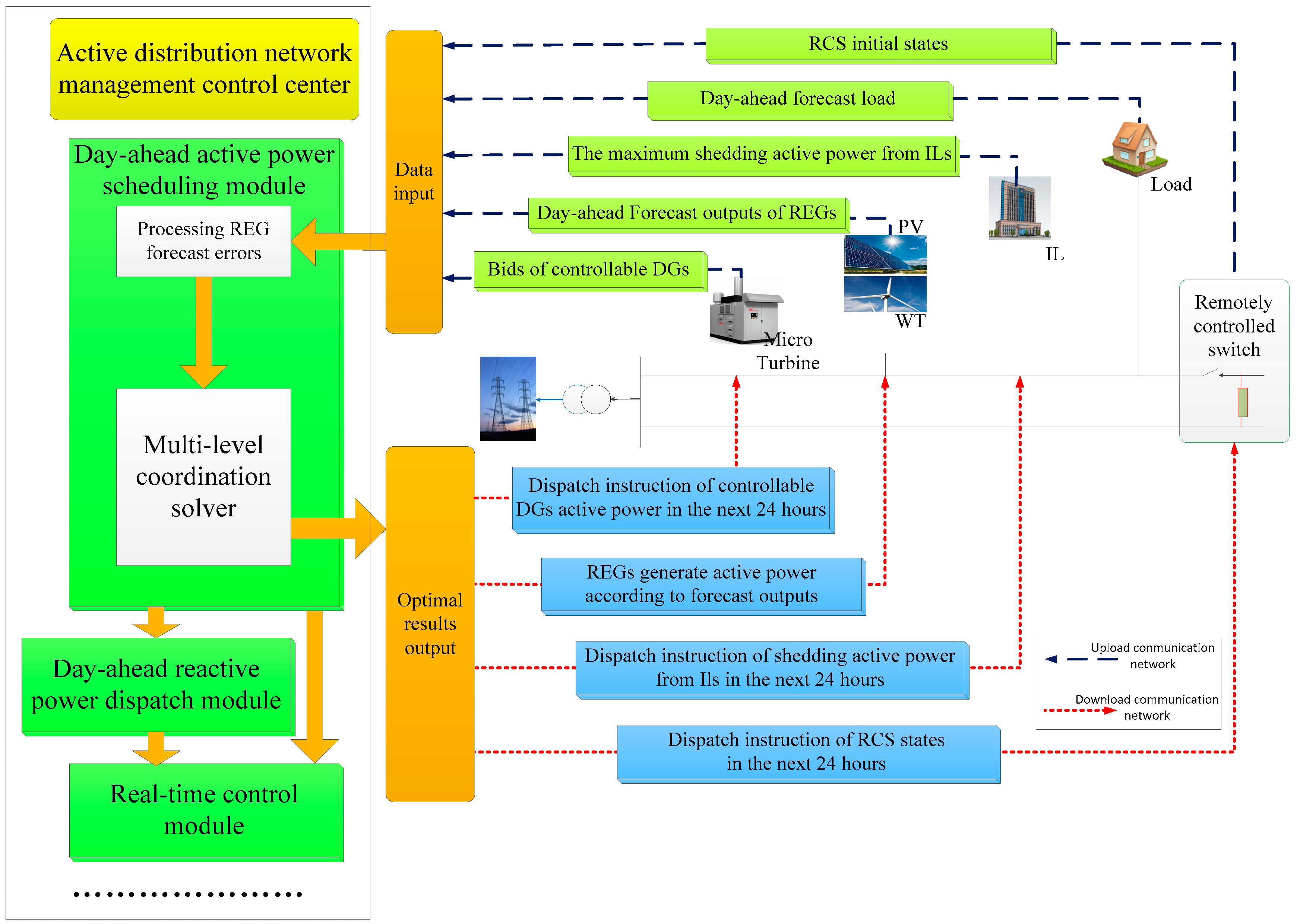
Firstly, an initial optimization model is established to preliminarily optimize DER outputs and RCS states statically in each hour. However, the hourly optimal results of RCS states may cause frequent switching. Therefore, RCS states need to be optimized secondly considering a limited switching number in one day. Thirdly, DER outputs are optimized based on the optimal result in RCS optimization, in order to mitigate the extra cost caused by the updated RCS states. Finally, the RCS optimization and DER optimization iterate mutually until convergence criterion is achieved, when the optimal results of RCS and DER optimization won’t change with iterations. CCP is adopted to deal with the multi-state models of REG outputs, and address the randomness due to REG forecast errors. The flowchart of the proposed hierarchical coordination optimization is shown as Figure 1.
In real implementation, the day-ahead active power scheduling method proposed in this paper is located at the ADNM control center and is implemented by DSOs. DSOs acquire RCS initial states, day-ahead forecast load, the maximum shedding active power from ILs, day-ahead forecast outputs of REGs, day-ahead bids of controllable DGs through upload communication networks. According REG forecast errors, day-ahead forecast outputs of REGs are processed by the multi-state model. Then the optimal results can be achieved in multi-level coordination solver by the hierarchical coordination optimization method based on CCP. Taking the optimal results as the dispatch instructions, DSOs delivery the dispatch instructions to the controllable devices, including DER outputs and RCS states in the next 24 h, by the download communication networks. REGs generate active power according to their day-ahead forecast outputs in order to take full advantages of renewable energies and reduce carbon emissions. Day-ahead reactive power dispatch and real-time control, which also are important modules in the ADNM control centre, are implemented after day-ahead active power scheduling. Providing the day-ahead dispatch instructions for real-time control, day-ahead scheduling is the basis of real-time control. Real-time control updates the day-ahead dispatch instructions and determines the actual operations of controllable resources. The practical implementation of day-ahead active power scheduling is shown as Figure 2.
3.1. Initial Optimization
Based on the multi-state models of WT-PV outputs in each hour, the controllable DGs outputs, the shedding powers from ILs and the RCS states of each hour are optimized, respectively, taking the operation costs of distribution companies (DISCOs) as optimization objective. The operation costs contain the cost of power purchases from the grid (), cost of power purchases from DGs (), cost of compensation DGs () and cost of compensation ILs (). Chance constrained programming [26] is adopted to deal with the multi-state models of WT-PV outputs. CCP can be used to solve the optimization problem with uncertain factors under the given confidence level, which is suitable for solving the scheduling problem in this paper that takes the uncertain outputs of REGs into consideration.
In t period, the objective is formulated as follows:
The constraints are as follows:
- (1)
- Probability constraint of the objectivewhere x is the decision variable, including the controllable DGs outputs, the shedding powers of ILs and the RCS states (open or closed); is the state variable in the multi-state system; is the maximum number of state variables; is the operation cost in state ; is the probability when the condition in is satisfied; α is the confidence level; is the minimum value when the probability level of is more than α; is one hour in this paper; is the active power purchases from the grid in t period; is the unit cost of the active power purchases; G is the set of DGs including controllable DGs and uncontrollable ones; is the active power of the mth DG in t period that DMS allows producing on the basis of the optimization result; is the unit cost of the active power purchases from the mth DG; is the bid of active power; is the compensation cost for cutting 1 kWh of the mth DG; C is the set of ILs; is the shedding power from the vth IL in t period; is the compensation cost for cutting 1 kWh of the vth IL; is the selling cost of DISCOs in t period.
- (2)
- Probability constraint of branch power:where is the active power of branch in state ; is the maximum power of branch ; is the confidence level of branch power.
- (3)
- Probability constraint of node voltage:where is the voltage of node i in state ; and are the maximum and minimum voltage of node i respectively; is the confidence level of node voltage.
- (4)
- Constraint of energy balance:where is the set of controllable DGs, and is the set of uncontrollable ones; is the active power output of the th controllable DG in t period, and is the output of the th uncontrollable one; is the total load in t period; is the network loss in t period.
- (5)
- Constraint of active and reactive power balance:where , are active and reactive power injection of bus i; and are voltages of i and j; and are real part and imaginary part of admittance matrix; is phase angle difference between i and j.
- (6)
- Constraint of the controllable DG outputs:where and are the minimum and maximum output of the th controllable DG in t period, respectively. In real implementation, the 24-h maximum active power outputs of controllable DGs are set as their day-ahead bids of active power provided by the DG owners.
- (7)
- Constraint of the exploitation of ILs:where t’ is the period when load is heavy; where and are the minimum and maximum shedding active power from the vth IL in t’ period, respectively.
- (8)
- Constraint of power purchases from the grid:where and are the minimum and maximum active power purchases from the grid in t period.
- (9)
- Constraint of network topology:After reconfiguration, the network is still connected radially without the presence of islanding.
3.2. RCS Optimization
The initial optimization results are the ideal ones without considering the limited number of RCS switching actions, however frequent switching actions will increase the wear and tear on RCSs, and the loop closing operation during the course of reconfiguration may lead to larger loop current [27]. Hence, RCSs cannot be operated frequently in one day, and the RCS states need to be re-optimized with the constraint of the maximum number of RCS switching actions in 24 h [28].
First of all, the periods with the same RCS states are merged according to the initial optimization results, as a consequence, T periods are combined into L new ones (). Then considering the limited number and cost of RCS switching actions, the network topologies are adjusted according to the initial optimization results in the merged periods. A dynamic reconfiguration network model is established taking the costs of network loss and switching action as optimization objective:
where is the total number of RCSs; T is the period number, set as 24 in this paper; is the number of the merged periods; is the cost of one switching action; is the state of the kth RCS in period, and means open, means closed.
The constraints are as follows:
- (1)
- Constraint of the maximum number of RCS switching actions:where is the maximum number of single RCS switching actions; is the maximum number of total RCS switching actions.
- (2)
- Constraint of node voltage:
- (3)
- Constraint of branch power:
Besides, the constraints of active and reactive power balance and network topology in RCS optimization are the same with the ones in initial optimization.
3.3. DER Optimization
The adjustment of network topologies will change the distribution and direction of power flow, which affects the optimal outputs of DERs, thus DER optimization is needed to acquire the new optimization results of DERs with the solution of RCS optimization. The outputs of controllable DGs and the exploitation of ILs in each period are optimized with an optimization objective of the operation costs of DISCOs, and CCP is employed to solve the multi-state models of WT-PV outputs.
The constraints are as follows:
Probability constraint of the objective:
where the decision variable includes the controllable DGs outputs and the exploitation of ILs without the RCS states, which is different from initial optimization.
Besides, the other constraints of DER optimization are same with constraints (2)–(8) of initial optimization.
From the above Section 3.1, Section 3.2 and Section 3.3, the hierarchical coordination optimization method can ensure an optimal solution of RCS states and DER outputs for 24 h. In initial optimization (Section 3.1), hourly optimal solution of RCS states and DER outputs can be achieved by optimizing DER outputs and RCS states statically in each hour. However, the result of initial optimization is not the global optimal solution without considering the daily limited number of RCS switching actions. The global optimal solution can be acquired with mutual iterations of RCS optimization (Section 3.2) and DER optimization (Section 3.3), which takes the constraint of daily maximum number of RCS switching actions into the optimization model (Section 3.2).
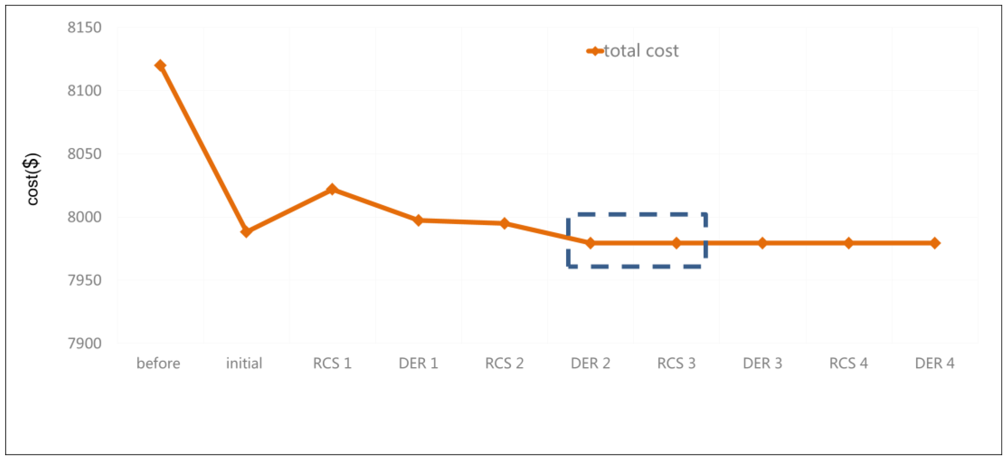
Furthermore, a fast convergence speed can be guaranteed with the proposed method. There are two main reasons for the rapid convergence. One reason is that the huge solution space of the MP-MINLO problem is narrowed effectively in initial optimization, which optimizes DER outputs and RCS states statically in each hour and serves its optimization results as the initial values of other two levels. Initial optimization improves searching efficiency of RCS optimization and DER optimization. The other reason is that the model of each level takes network losses as a part of the optimization goal, and all three levels pursue the optimal economic efficiency. As a result, the search direction of three levels is consistent, which ensures that the results can converge to the global optimal solution rapidly in process of solving. The convergence speed result is shown in Section 5.4 with Figure 10.
4. Optimization Algorithm
As a complex MP-MINLO problem, the hierarchical coordination optimization model proposed in this paper can be solved by a hybrid particle swarm optimization (PSO) algorithm. The hybrid PSO algorithm [28] has good robustness and fast convergence speed, and it can optimize discrete variables (RCS states) and continuous variables (DER outputs) concurrently in one period. Reference [28] is consulted in the respects of network topology simplification, keeping the radial network topology, single particle encoding and the update of particle velocity and position, and the details will not be mentioned in this paper. Compared with reference [28], the hierarchical optimization coordination model is adopted in this paper, therefore the single particle encoding objects in each level are different, and the details will be given in Section 4.1. In addition, considering CCP in the model, hybrid PSO algorithm needs to be improved and Section 4.2 will give details.
4.1. Single Particle Encoding Method in Hybrid PSO
In initial optimization, it is necessary to optimize RCS states and DER outputs at the same time. Set the number of RCSs as , the number of controllable DGs as , the number of ILs as , and each particle encoded representation in t period can be shown as Equation (29):
In RCS optimization, only RCS states are optimized. Set the number of merged periods as , and each particle encoded representation can be shown as Equation (30):
In DER optimization, only the controllable DGs outputs and ILs reduction are coded due to the fixed RCSs, and each particle encoded representation can be shown as Equation (31):
4.2. Chance-Constrained Programming
CCP is used to deal with REG forecast errors in the model, so the hybrid PSO algorithm is improved to acquire the optimization results satisfying the confidence level. In initial optimization and DER optimization, aiming at M states of WT-PV outputs, the model is solved M times circularly in each period, and we sort the M calculated objective values from the best to the worst. The probability is accumulated in order until the probability accumulation reaches the confidence level, and the corresponding result is the optimal solution. Taking the optimization process in t period in initial optimization as an example, the solver with CCP is shown as Figure 3.
5. Case Studies
In this section, four cases will be introduced to demonstrate the benefits for coordination optimization of network reconfiguration and DER outputs, consideration of REG forecast errors and the hierarchical coordination optimization method, respectively.
5.1. Test System Specifications
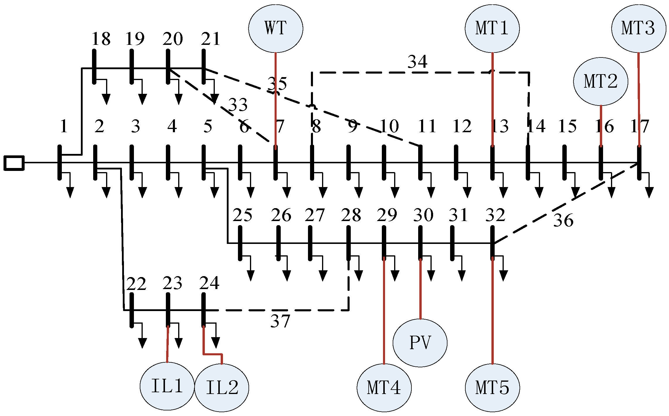
The improved IEEE 33 nodes distribution network [29] is adopted as the test system, shown as Figure 4. Each branch is equipped with a RCS. The maximum daily number of each RCS switching actions () is 6, and the total number () is 30 [19]. Node 13, 16, 17, 29 and 32 are provided with a MT respectively, with 390 kW rated power; Node 23 and 24 are two industrial loads which participate as ILs, and the maximum shedding active power is 350 kW, which is lower than the actual active power needs of Node 23 and 24. Node 7 and node 30 are provided a WT and a PV respectively, and the power rating of the WT is 300 kW, while the power rating of the PV is 400 kW. The period of heavy load is from 6 p.m. to 10 p.m., and ILs can only be shed in this period. The outputs of the WT, the PV and loads can be forecasted by the historical data in Shandong Province, China. The REG forecast errors obey a Gaussian distribution, and the practical operating data is shown as Figure 5. Values of some price parameters are shown as Table 1.
The population size of PSO is 50, and the number of iterations is 100. The confidence level of objective function, branch power and node voltage in CCP is 0.9. Four cases will be solved by Matlab 2012a version on an i5-3230M CPU, 8 G RAM computer. There are four cases designed to verify the validity of the method proposed in this paper:
- Case 1:
- Scheduling of DER outputs only considering REG forecast errors. In this case, DER outputs in each period are optimized with the fixed network topologies, and PSO is used to solve this case.
- Case 2:
- Coordination scheduling of RCS states and DER outputs considering REG forecast errors. In this case, day-ahead coordination optimization of network reconfiguration and DER outputs is implemented by the method mentioned in this paper.
- Case 3:
- Coordination scheduling of RCS states and DER outputs without considering REG forecast errors. In this case, the outputs of WT and PV are determinate and the hierarchical coordination optimization without CCP is employed.
- Case 4:
In Section 5.2, the optimization results of Case 1 and Case 2 are analyzed to verify the benefits for coordination optimization of network reconfiguration and DER outputs. In Section 5.3, the optimization results of Case 2 and Case 3 are analyzed to verify the benefits considering REG forecast errors. In Section 5.4, the optimization results of Case 2 and Case 4 are analyzed to verify the benefits for the hierarchical coordination optimization method.
5.2. Benefits for Coordination Optimization of Network Reconfiguration and DER Outputs
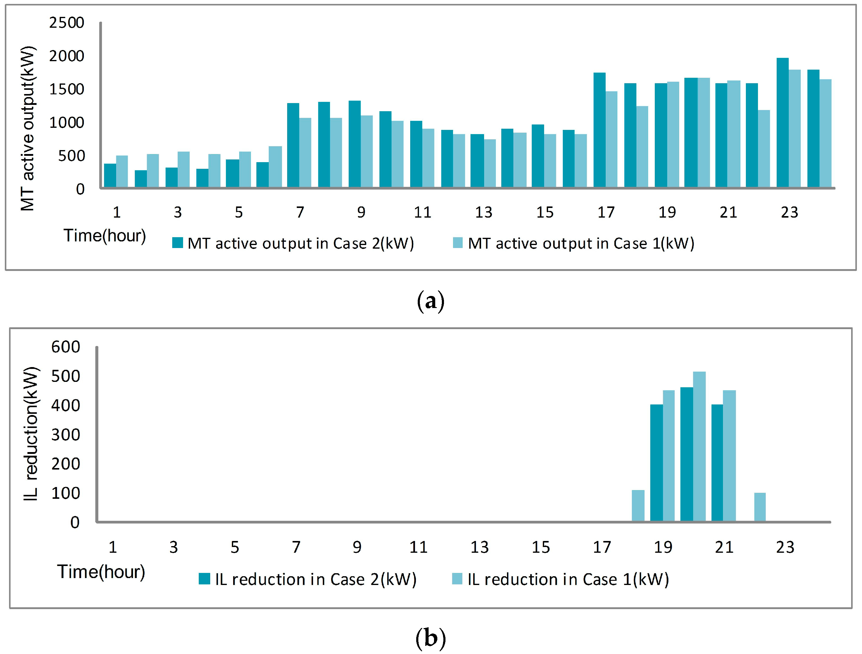
The analysis of the optimization results of Case 1 and Case 2 in Figure 6, Table 2 and Table 3 is indicated below:
- (1)
- Comparative discussions of Case 1 and Case 2. In Figure 6a, the total active power outputs of MTs of Case 2 are 25,990 kWh in a day, while the ones of Case 1 are 24,540 kWh. Compared with Case 1, the MTs outputs of Case 2 increase by 5.9%. In Figure 6b, the total exploitation of ILs of Case 2 is 1260 kWh, while the one of Case 1 is 1620 kWh within one day. Compared with Case 1, the ILs reduction of Case 2 decreases by 22.2%. The above analysis shows that the scheduling of RCS states can increase DGs penetration, reduce the load exploitation of consumer side, enhance the absorption ability of distribution network to DGs and improve the reliability of power supply.
- (2)
- Analysis of the optimization results of Case 2. When the load level is low (1 a.m. to 4 p.m.), the main optimizing way is the adjustment of MTs outputs, and ILs are not involved in the scheduling, with fewer RCS switching operations (four times from Table 2); when the load level is high (5 p.m. to 12 p.m.), the outputs of WT and PV decrease, as a consequence, MTs output and ILs reduction increase significantly, and frequent RCS switching operations occur (eight times from Table 2), which illustrates that the coordination scheduling of network topologies and DER outputs is needed at this moment. From Table 3, the total operation cost of Case 2 is lower compared with Case 1, which shows that the coordinated scheduling of RCS states and DER outputs can improve the economic benefit of DISCOs.
5.3. Benefits for Considering REG Forecast Errors
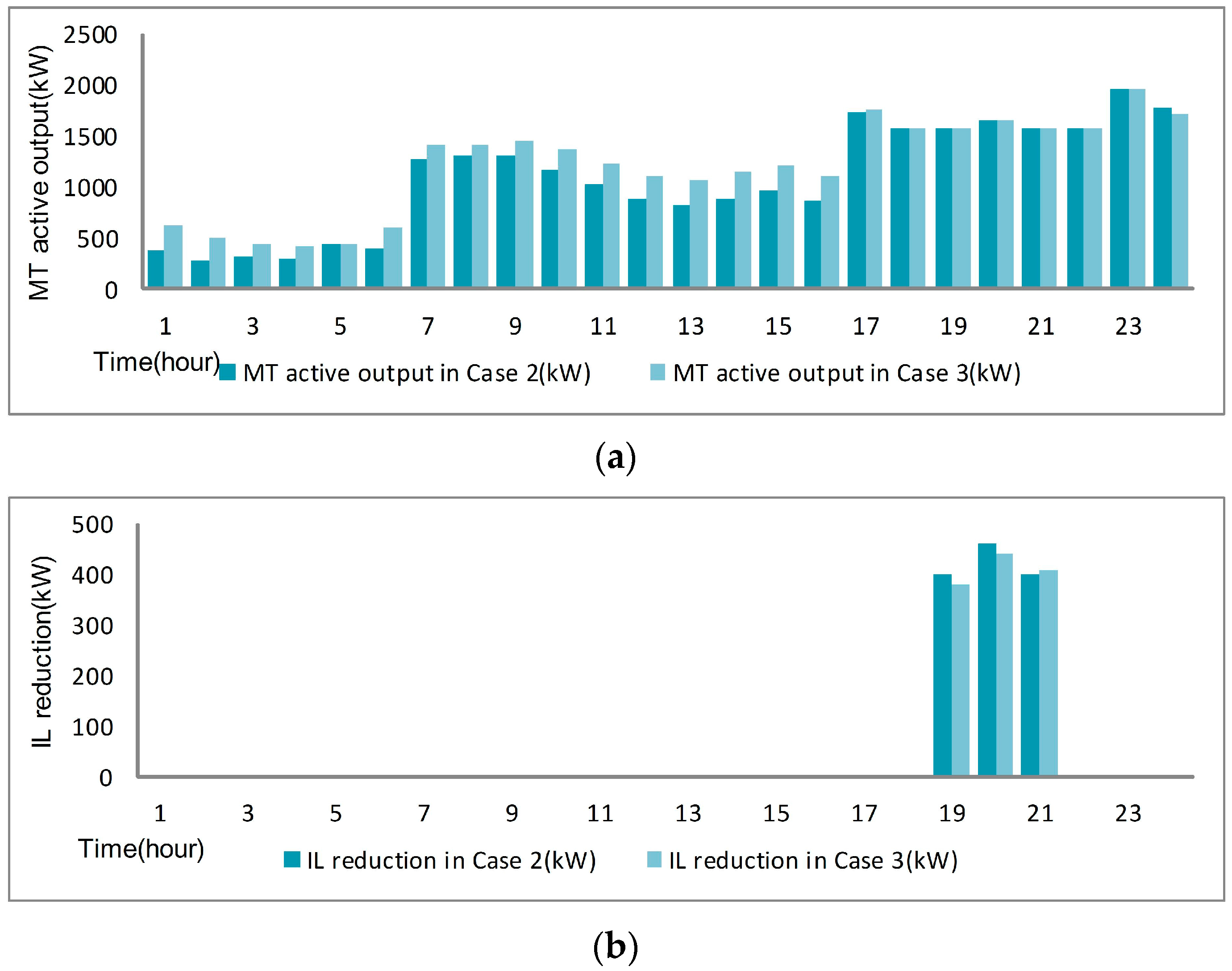
In Case 2, CCP is used to deal with the impact of REG forecast errors on optimization results. Case 3 doesn’t consider REG forecast errors and the outputs of WT and PV are determinate. We optimize Case 2 and Case 3 to achieve the optimal solutions, and the optimization results of Case 2 and Case 3 are shown as Figure 7 and Table 4.
To test the benefits for considering REG forecast errors, risk index of undervoltage and overvoltage is defined in this section. It is assumed that there are N stochastic scenarios. The optimal schemes of Case 2 and Case 3 are used for power flow calculation in these stochastic scenarios respectively. The number of undervoltage (lower than 0.93) and overvoltage (higher than 1.07) episodes in one scheme in t period can be obtained, which is set as . Then is defined as the risk index of undervoltage and overvoltage. In this process, Monte Carlo Simulation (MCS) [31] is used as a sampling method to generate the stochastic according to the hourly probability density function of REG forecast errors. Figure 8 demonstrates the hourly results of the risk index of undervoltage and overvoltage in Case 2 and Case 3, and the simulation number of stochastic scenarios is 10,000 times.
The analysis of the above optimization results is as follows:
- (1)
- In Table 2, the RCS switching action number of Case 2 is similar to that of Case 3, which illustrates that considering REGs forecast errors has little influence on reconfiguration. In Figure 7, when REG outputs are high (1 a.m. to 4 p.m.), the difference of MTs generation between Case 2 and Case 3 is relatively larger; When REG outputs are low (5 p.m. to 12 p.m.), the difference of MTs generation between Case 2 and Case 3 is smaller, which indicates that REG forecast errors surely have effect on the prioritization scheme. In Table 4, the total operation cost of Case 3 decreases by $3 compared with Case 2, which shows that in order to ensure the power supply quality and resist the influence of REG forecast errors, the operation cost is increased by CCP, but the cost only increases by 0.039% and it is acceptable.
- (2)
- In Figure 8, the risk index of undervoltage and overvoltage in Case 3 is much higher than that in Case 2 in each hour. The highest risk index within one day in Case 3 is 0.37, higher than that in Case 2 by 413.9%. The 24-h average value of the risk index in Case 3 is 0.173, higher than that in Case 2 by 380.6%. It illustrates that the proposed method in this paper can significantly reduce the risk of undervoltage and overvoltage due to REG forecast errors, and improve the power supply quality and security of distribution network.
5.4. Benefits for the Hierarchical Coordination Optimization Method
The hierarchical coordination optimization method is used to dispatch DER outputs and RCS states in Case 2. In Case 4, hybrid integer genetic algorithm from reference [19] is employed to realize a comprehensive optimization scheduling of network topologies and DER outputs. The comparisons of optimization results of Case 4 and Case 2 are shown in Figure 9 and Table 5.
In Case 4, the total generation of MTs is 22,060 kWh in one day, reducing by 15.12% compared with that in Case 2; the total ILs reduction in Case 4 is 2270 kWh, increasing by 80.16% compared with that in Case 2. In Table 2, the number of RCS switching action is 28 in one day in Case 4, increasing 16 times compared with that in Case 2, which shows that the method of Case 2 can decrease the number of RCS switching action effectively compared with that of Case 4. In Table 5, the loss cost and the total cost in Case 2 are less than that in Case 4. The main reason for this situation is that the proposed hierarchical coordination optimization procedure used in Case 2 is a more effective method to reduce solution space than hybrid integer GA used in Case 4. The optimization variables of this problem contain RCS states of 24 h, DGs outputs of 24 h and ILs reduction of 24 h, making the solution space really huge. Hybrid integer GA optimizes all the variables simultaneously so the search efficiency of is decreased rapidly and it is easy to run into local optimum. However, in the hierarchical coordination optimization procedure, initial optimization dispatches DER outputs and RCS states statically in each hour, which decomposes one huge solution space into 24 smaller solution spaces. Initial optimization can easily obtain 24 better solutions. RCS optimization and DER optimization optimize discrete and continuous variables respectively, so dimension of variables is decreased. Continuous and discrete variables are optimized separately in an efficient way. All the three levels can narrow the solution space and improve searching efficiency. Therefore, a better optimization result can be acquired with the proposed method in this paper.
Each level in the hierarchical coordination optimization model is optimized to achieve the minimum operation cost, so the convergence rate is fast. Figure 10 shows the optimal objective values during the iterative process in Case 2 and convergence can be realized in the third iteration.
Finally, CPU times for each case are shown as Table 6. We can see that the execution speeds of Case 1 and Case 3 are faster than that of Case 2 and Case 4. This is because that Case 1 ignores the optimization of RCSs and Case 3 does not consider REG forecast errors, which reduce the computational burden of Case 1 and Case 3. The execution speed of Case 2 is a little slower than that of Case 4. This is because the iterative process between three levels needs more time. Even so, CPU time of Case 2 can be acceptable, because the requirement for execution speed is not very high and the accuracy of optimization has a higher priority regarding a day-ahead optimization problem.
6. Conclusions
This paper presents a day-ahead coordination optimization scheduling method for ADNs, in which REG forecast errors are considered, and a hierarchical coordination optimization model is addressed to coordinate DER outputs and network topologies. The conclusions of this paper are as follows:
- (1)
- The coordination scheduling of network topologies and DER outputs can effectively cope with the load variation in 24 h, improve the economic efficiency of DISCOs, and achieve the comprehensive utilization of the assets in ADNs. Network reconfiguration can increase DG penetrations, and reduce the load exploitation of consumer side.
- (2)
- Multi-state models and CCP are adopted in the stochastic scheduling model, which can decrease the serious influence of REG forecast errors on optimal scheduling results. Although the operation cost is increased slightly with the method mentioned in this paper, the risk of undervoltage and overvoltage caused by REG forecast errors can be reduced significantly, and the reliability and safety of power supply can be improved.
- (3)
- The hierarchical coordination optimization method can consider the constraint of the daily number of RCS switching actions, realize the coordination scheduling of RCS states and DER outputs, reduce the solution space greatly and solve the MP-MINLO problem effectively. In this method, initial optimization provides preliminary values for RCS optimization, based on which optimal RCS states can be searched efficiently. RCS optimization can avoid frequent switching actions. Based on optimal RCS states, the DER outputs are adjusted by DER optimization. An optimal solution can be achieved finally through iterations between RCS and DER optimization.
Acknowledgments
This work was supported by National Natural Science Foundation of China under Grant 51377162.
Author Contributions
The paper was a collaborative effort between the authors. Pengwei Cong designed the hierarchical coordination optimization model, Wei Tang contributed to the optimization algorithm, Lu Zhang contributed to the modeling of REG forecast errors, Bo Zhang and Yongxiang Cai did the case studies.
Conflicts of Interest
The authors declare no conflict of interest.
Nomenclature
| DER | Distributed Energy Resource |
| ADN | Active Distribution Network |
| REG | Renewable Energy Generation |
| DG | Distributed Generation |
| EES | Electrical energy storage |
| CL | Controllable Load |
| ICT | Information and Communication Technologies |
| DSO | Distribution system operator |
| WT | Wind Turbine |
| PV | Photovoltaic |
| MT | Micro Turbine |
| ADNM | Active Distribution Network Management |
| RCS | Remotely Controlled Switch |
| OPF | Optimal Power Flow |
| MP-MINLO | Multi-period Mixed Integer Nonlinear Optimization |
| CCP | Chance Constrained Programming |
| Probability Density Function | |
| DISCO | Distribution Company |
| PSO | Particle Swarm Optimization |
| MCS | Monte Carlo Simulation |
References
- Chen, F.; Liu, D.; Xiong, X. Research on Stochastic Optimal Operation Strategy of Active Distribution Network Considering Intermittent Energy. Energies 2017, 10, 522. [Google Scholar] [CrossRef]
- Saponara, S.; Bacchillone, T. Network Architecture, Security Issues, and Hardware Implementation of a Home Area Network for Smart Grid. J. Comput. Netw. Commun. 2012, 2012, 534512. [Google Scholar] [CrossRef]
- Costantino, N.; Serventi, R.; Tinfena, F.; D’Abramo, P.; Chassard, P.; Tisserand, P.; Saponara, S.; Fanucci, L. Design and Test of an HV-CMOS Intelligent Power Switch With Integrated Protections and Self-Diagnostic for Harsh Automotive Applications. IEEE Trans. Ind. Electron. 2011, 58, 2715–2727. [Google Scholar] [CrossRef]
- Saponara, S.; Fanucci, L.; Bernardo, F.; Falciani, A. Predictive Diagnosis of High-Power Transformer Faults by Networking Vibration Measuring Nodes with Integrated Signal Processing. IEEE Trans. Instrum. Meas. 2016, 65, 1749–1760. [Google Scholar] [CrossRef]
- Tan, Y.; Cao, Y.; Li, Y.; Lee, K.; Jiang, L.; Li, S. Optimal Day-Ahead Operation Considering Power Quality for Active Distribution Networks. IEEE Trans. Autom. Sci. Eng. 2017, 14, 425–436. [Google Scholar] [CrossRef]
- Hu, Z.; Li, F. Cost-Benefit analyses of active distribution network management, part I: Annual benefit analysis. IEEE Trans. Smart Grid 2012, 3, 1067–1074. [Google Scholar] [CrossRef]
- Zhang, J.; Fan, H.; Tang, W.; Wang, M.; Cheng, H.; Yao, L. Planning for distributed wind generation under active management mode. Int. J. Electric Power Energy Syst. 2013, 47, 140–146. [Google Scholar] [CrossRef]
- Deshmukh, S.; Natarajan, B.; Pahwa, A. Voltage/VAR control in distribution networks via reactive power injection through distributed generators. IEEE Trans. Smart Grid 2012, 3, 1226–1234. [Google Scholar] [CrossRef]
- Niknam, T.; Narimani, M.R.; Azizipanah-Abarghooee, R. Multiobjective Optimal Reactive Power Dispatch and Voltage Control: A New Opposition-Based Self-Adaptive Modified Gravitational Search Algorithm. IEEE Syst. J. 2013, 7, 742–753. [Google Scholar] [CrossRef]
- Gill, S.; Kockar, I.; Ault, G.W. Dynamic optimal power flow for active distribution networks. IEEE Trans. Power Syst. 2014, 29, 121–131. [Google Scholar] [CrossRef] [Green Version]
- Flaih, F.M.F.; Lin, X.; Abd, M.K.; Dawoud, S.M.; Li, Z.; Adio, O.S. A New Method for Distribution Network Reconfiguration Analysis under Different Load Demands. Energies 2017, 10, 455. [Google Scholar] [CrossRef]
- D’Adamo, C.; Jupe, S.; Abbey, C. Global survey on planning and operation of active distribution networks—Update of CIGRE C6.11 working group activities. In Proceedings of the 20th International Conference on Electricity Distribution (CIRED 2009), Prague, Czech, 8–11 June 2009; pp. 1–4. [Google Scholar]
- Rao, R.S.; Ravindra, K.; Satish, K.; Narasimham, S. Power loss minimization in distribution system using network reconfiguration in the presence of distributed generation. IEEE Trans. Power Syst. 2013, 28, 317–325. [Google Scholar] [CrossRef]
- Malekpour, A.R.; Niknam, T.; Pahwa, A.; Fard, A. Multi-objective stochastic distribution feeder reconfiguration in systems with wind power generators and fuel cells using the point estimate method. IEEE Trans. Power Syst. 2013, 28, 1483–1492. [Google Scholar] [CrossRef]
- Khodaei, A. Microgrid optimal scheduling with multi-period islanding constraints. IEEE Trans. Power Syst. 2014, 29, 1383–1392. [Google Scholar] [CrossRef]
- Borghetti, A.; Bosetti, M.; Grillo, S.; Massucco, S.; Nucci, C.; Paolone, M.; Silvestro, F. Short-Term scheduling and control of active distribution systems with high penetration of renewable resources. IEEE Syst. J. 2010, 4, 313–322. [Google Scholar] [CrossRef]
- Pilo, F.; Pisano, G.; Soma, G.G. Optimal coordination of energy resources with a two-stage online active management. IEEE Trans. Ind. Electron. 2011, 58, 4526–4537. [Google Scholar] [CrossRef]
- Celli, G.; Pilo, F.; Pisano, G.; Soma, G.G. Optimal operation of active distribution networks with Distributed Energy Storage. In Proceedings of the IEEE International Energy Conference and Exhibition (ENERGYCON), Florence, Italy, 9–12 September 2012; pp. 557–562. [Google Scholar]
- Golshannavaz, S.; Afsharnia, S.; Aminifar, F. Smart distribution grid: Optimal day-ahead scheduling with reconfigurable topology. IEEE Trans. Smart Grid 2014, 5, 2402–2411. [Google Scholar] [CrossRef]
- Zhang, Z.; Sun, Y.; Gao, D.; Lin, J.; Cheng, L. A versatile probability distribution model for wind power forecast errors and its application in economic dispatch. IEEE Trans. Power Syst. 2013, 28, 3114–3125. [Google Scholar] [CrossRef]
- Chen, N.; Qian, Z.; Nabney, I.T.; Meng, X. Wind power forecasts using Gaussian processes and numerical weather prediction. IEEE Trans. Power Syst. 2014, 29, 656–665. [Google Scholar] [CrossRef]
- Capitanescu, F.; Ochoa, L.F.; Margossian, H.; Hatziargyriou, N. Assessing the potential of network reconfiguration to improve distributed generation hosting capacity in active distribution systems. IEEE Trans. Power Syst. 2015, 30, 346–356. [Google Scholar] [CrossRef]
- Fan, M.; Vittal, V.; Heydt, G.T.; Ayyanar, R. Probabilistic power flow analysis with generation dispatch including photovoltaic resources. IEEE Trans. Power Syst. 2013, 28, 1797–1805. [Google Scholar] [CrossRef]
- Wang, R.; Li, W.; Bagen, B. Development of wind speed forecasting model based on the Weibull probability distribution. In Proceedings of the International Conference on Computer Distributed Control and Intelligent Environmental Monitoring (CDCIEM), Changsha, China, 19–20 February 2011; pp. 2062–2065. [Google Scholar]
- Karaki, S.H.; Chedid, R.B.; Ramadan, R. Probabilistic performance assessment of autonomous solar-wind energy conversion systems. IEEE Trans. Energy Convers. 1999, 14, 766–772. [Google Scholar] [CrossRef]
- Yu, H.; Chung, C.; Wong, K.; Zhang, J. A chance constrained transmission network expansion planning method with consideration of load and wind farm uncertainties. IEEE Trans. Power Syst. 2009, 24, 1568–1576. [Google Scholar] [CrossRef]
- Loos, M.; Werben, S.; Maun, J.C. Circulating currents in closed loop structure, a new problematic in distribution networks. In Proceedings of the IEEE Power and Energy Society General Meeting, San Diego, CA, USA, 22–26 July 2012; pp. 1–7. [Google Scholar]
- Chen, S.; Hu, W.; Chen, Z. Comprehensive cost minimization in distribution networks using segmented-time feeder reconfiguration and reactive power control of distributed generators. IEEE Trans. Power Syst. 2016, 31, 1–11. [Google Scholar] [CrossRef]
- Baran, M.E.; Wu, F. Network reconfiguration in distribution system for loss reduction and load balancing. IEEE Trans. Power Del. 1989, 4, 1401–1407. [Google Scholar] [CrossRef]
- Outdoor Medium Voltage Automatic Circuit Reclosers. Available online: http://www.alibaba.com/product-detail/33KV-automatic-circuit-recloserACR_1673941121.html (accessed on 12 June 2016).
- Mokryani, G.; Siano, P. Combined Monte Carlo simulation and OPF for wind turbines integration into distribution networks. Electric Power Syst. Res. 2013, 103, 37–48. [Google Scholar] [CrossRef]
Figure 1.
The flow chart of the hierarchical coordination optimization. WTs: wind turbines; PVs: photovoltaics; DERs: distributed energy resource; RCSs: remotely controlled switches.
Figure 1.
The flow chart of the hierarchical coordination optimization. WTs: wind turbines; PVs: photovoltaics; DERs: distributed energy resource; RCSs: remotely controlled switches.
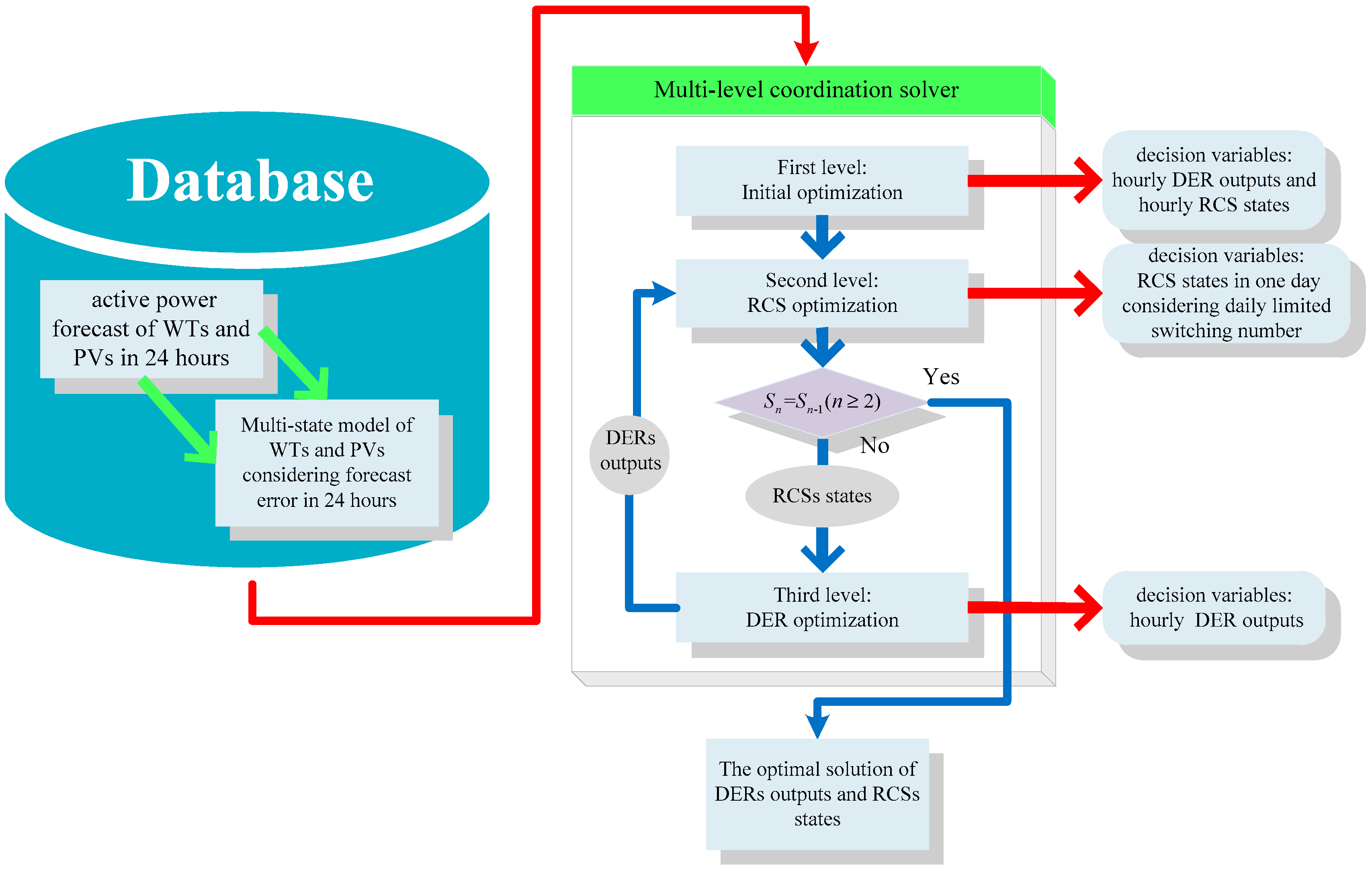
Figure 2.
The practical implementation of day-ahead active power scheduling. DG: distributed generation; REG: renewable energy generation.
Figure 2.
The practical implementation of day-ahead active power scheduling. DG: distributed generation; REG: renewable energy generation.

Figure 3.
The flow chart of chance constrained programming (CCP).
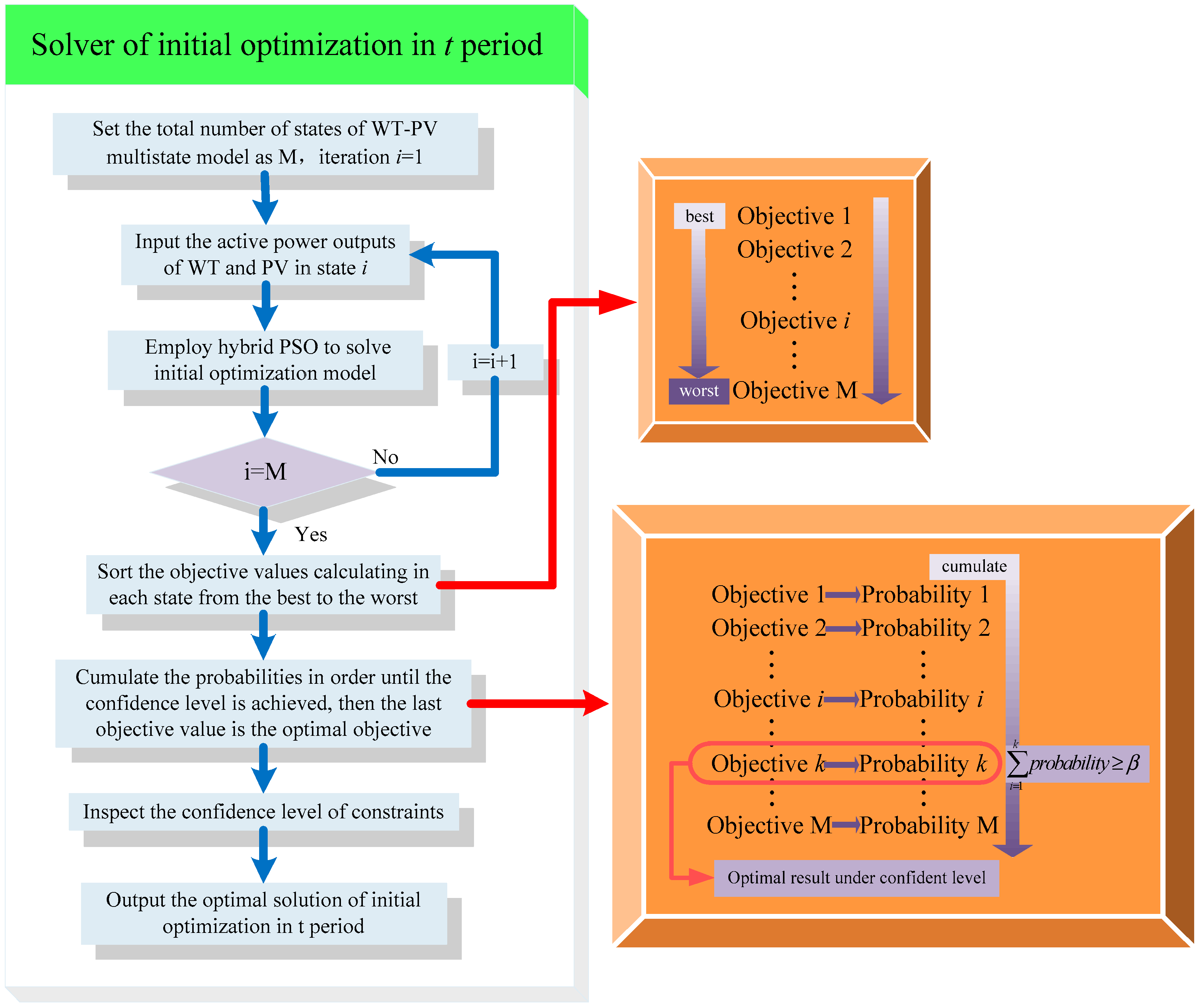
Figure 4.
IEEE 33 nodes distribution system integrated DERs.

Figure 5.
The practical operating data.
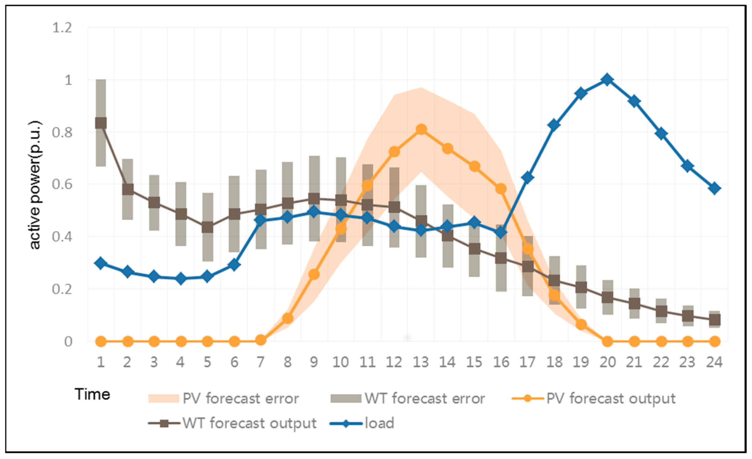
Figure 6.
Comparisons of DER outputs in each hour between case 1 and case 2. (a) Comparison of MTs active power outputs in each hour between case 1 and case 2; (b) Comparison of ILs reduction in each hour between case 1 and case 2.
Figure 6.
Comparisons of DER outputs in each hour between case 1 and case 2. (a) Comparison of MTs active power outputs in each hour between case 1 and case 2; (b) Comparison of ILs reduction in each hour between case 1 and case 2.

Figure 7.
Comparisons of DER outputs in each hour between Case 2 and Case 3. (a) Comparison of MTs active power outputs in each hour between Case 2 and Case 3; (b) Comparison of ILs reduction in each hour between Case 2 and Case 3.
Figure 7.
Comparisons of DER outputs in each hour between Case 2 and Case 3. (a) Comparison of MTs active power outputs in each hour between Case 2 and Case 3; (b) Comparison of ILs reduction in each hour between Case 2 and Case 3.

Figure 8.
Risk of undervoltage and overvoltage in Case 2 and Case 3.
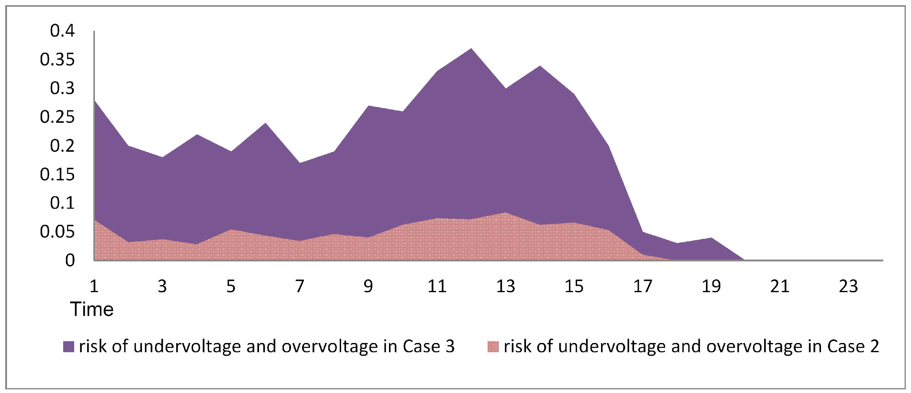
Figure 9.
Comparisons of DER outputs in each hour between case 2 and case 4. (a) Comparison of MTs active power outputs in each hour between case 2 and case 4; (b) Comparison of ILs reduction in each hour between case 2 and case 4.
Figure 9.
Comparisons of DER outputs in each hour between case 2 and case 4. (a) Comparison of MTs active power outputs in each hour between case 2 and case 4; (b) Comparison of ILs reduction in each hour between case 2 and case 4.
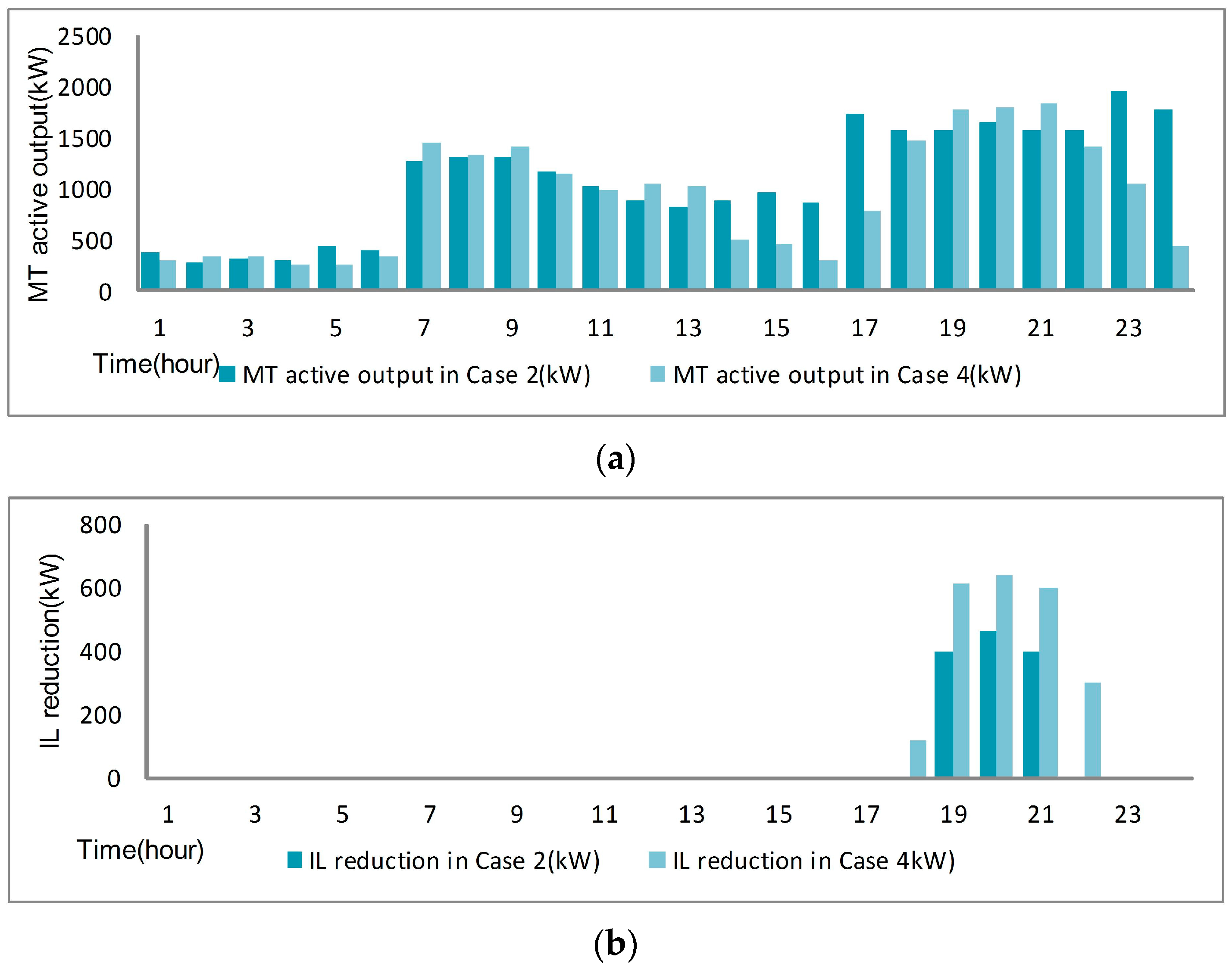
Figure 10.
Results during iterations in Case 2.

Table 1.
Values of some price parameters.
| Price Parameters | Values 1 |
|---|---|
| Electricity selling price () | $0.08/kWh |
| Purchase price from DGs () | $0.11/kWh |
| Compensation price for DGs () | $0.05/kWh |
| Purchase price from the grid () | $0.05/kWh |
| Compensation price for ILs () | $0.03/kWh |
| RCS switching action price [30] | $1/time |
1 The values are based on data from China.
Table 2.
Results of network reconfiguration.
| Time | Open RCSs in Case 2 | Open RCSs in Case 3 | Open RCSs in Case 4 |
|---|---|---|---|
| 1 | 9-15-33-34-37 | 9-15-33-34-37 | 9-36-33-34-26 |
| 2 | 9-15-33-34-37 | 9-15-33-34-37 | 9-36-33-34-26 |
| 3 | 9-15-33-34-37 | 9-15-33-34-37 | 9-36-33-34-26 |
| 4 | 9-15-33-34-37 | 9-15-33-34-37 | 9-36-33-34-26 |
| 5 | 9-15-33-34-37 | 9-15-33-34-37 | 12-21-33-34-37 |
| 6 | 9-15-33-34-37 | 9-15-33-34-37 | 12-21-33-34-37 |
| 7 | 9-13-33-34-28 | 9-12-15-33-37 | 12-21-33-34-37 |
| 8 | 9-13-33-34-28 | 9-12-15-33-37 | 9-36-33-34-26 |
| 9 | 9-13-33-34-28 | 9-12-15-33-37 | 9-36-33-34-26 |
| 10 | 9-13-33-34-28 | 9-12-15-33-37 | 9-36-33-34-26 |
| 11 | 9-13-33-34-28 | 9-14-33-34-28 | 9-36-33-34-26 |
| 12 | 9-13-33-34-28 | 9-14-33-34-28 | 9-36-33-34-26 |
| 13 | 9-13-33-34-28 | 9-14-33-34-28 | 9-36-33-34-26 |
| 14 | 9-13-33-34-28 | 9-14-33-34-28 | 9-36-33-34-26 |
| 15 | 9-13-33-34-28 | 9-14-33-34-28 | 9-36-33-34-26 |
| 16 | 9-13-33-34-28 | 9-14-33-34-28 | 11-14-33-34-37 |
| 17 | 9-16-33-34-28 | 9-16-33-34-28 | 11-14-33-34-37 |
| 18 | 9-16-33-34-28 | 9-16-33-34-28 | 11-14-33-34-37 |
| 19 | 9-16-33-34-28 | 9-16-33-34-28 | 10-16-33-34-37 |
| 20 | 9-16-33-34-28 | 9-16-33-34-28 | 10-16-33-34-37 |
| 21 | 9-16-33-34-28 | 9-16-33-34-28 | 10-16-33-34-37 |
| 22 | 9-16-33-34-28 | 9-16-33-34-28 | 10-14-33-34-26 |
| 23 | 9-12-15-33-37 | 9-16-33-34-28 | 10-14-33-34-26 |
| 24 | 9-12-15-33-37 | 9-16-33-34-28 | 10-14-33-34-26 |
| action number | 12 times | 10 times | 28 times |
Table 3.
Cost comparisons between case 1 and case 2.
| Solution Methods/Cost Indexes ($) | Case 1 | Case 2 |
|---|---|---|
| Loss cost | 124.20 | 91.26 |
| Switching action cost | 0 | 12 |
| Cost of paying to DGs | 4294.47 | 4372.38 |
| Purchase cost | 3546.96 | 3457.09 |
| Cost of paying to ILs | 176.51 | 137.28 |
| Total cost | 8017.94 | 7978.75 |
Table 4.
Cost comparisons between case 2 and case 3.
| Solution Methods/Cost Indexes ($) | Case 2 | Case 3 |
|---|---|---|
| Loss cost | 91.26 | 87.56 |
| Switching action cost | 12 | 10 |
| Cost of paying to DGs | 4372.38 | 4529.28 |
| Purchase cost | 3457.09 | 3302.42 |
| Cost of paying to ILs | 137.28 | 134.01 |
| Total cost | 7978.75 | 7975.71 |
Table 5.
Cost comparisons between case 2 and case 4.
| Solution Methods/Cost Indexes ($) | Case 2 | Case 4 |
|---|---|---|
| Loss cost | 91.26 | 111.68 |
| Switching action cost | 12 | 28 |
| Cost of paying to DGs | 4372.38 | 4161.22 |
| Purchase cost | 3457.09 | 3630.04 |
| Cost of paying to ILs | 137.28 | 247.33 |
| Total cost | 7978.75 | 8066.59 |
Table 6.
CPU times for each case.
| Case | CPU Times |
|---|---|
| Case 1 | 272 s |
| Case 2 | 570 s |
| Case 3 | 254 s |
| Case 4 | 520 s |
© 2017 by the authors. Licensee MDPI, Basel, Switzerland. This article is an open access article distributed under the terms and conditions of the Creative Commons Attribution (CC BY) license (http://creativecommons.org/licenses/by/4.0/).
Share and Cite
MDPI and ACS Style
Cong, P.; Tang, W.; Zhang, L.; Zhang, B.; Cai, Y. Day-Ahead Active Power Scheduling in Active Distribution Network Considering Renewable Energy Generation Forecast Errors. Energies 2017, 10, 1291. https://doi.org/10.3390/en10091291
AMA Style
Cong P, Tang W, Zhang L, Zhang B, Cai Y. Day-Ahead Active Power Scheduling in Active Distribution Network Considering Renewable Energy Generation Forecast Errors. Energies. 2017; 10(9):1291. https://doi.org/10.3390/en10091291
Chicago/Turabian StyleCong, Pengwei, Wei Tang, Lu Zhang, Bo Zhang, and Yongxiang Cai. 2017. "Day-Ahead Active Power Scheduling in Active Distribution Network Considering Renewable Energy Generation Forecast Errors" Energies 10, no. 9: 1291. https://doi.org/10.3390/en10091291
Note that from the first issue of 2016, this journal uses article numbers instead of page numbers. See further details here.