Modeling and Simulating Long-Timescale Cascading Faults in Power Systems Caused by Line-Galloping Events


1
Key Laboratory of Power System Intelligent Dispatch and Control of the Ministry of Education, Shandong University, Jinan 250061, China
2
China Electric Power Research Institute, Haidian District, Beijing 100192, China
*
Author to whom correspondence should be addressed.
Energies 2017, 10(9), 1301; https://doi.org/10.3390/en10091301
Submission received: 3 July 2017
/
Revised: 8 August 2017
/
Accepted: 23 August 2017
/
Published: 30 August 2017
(This article belongs to the Section F: Electrical Engineering)
Abstract
:With the increasing occurrence of extreme weather events, the short circuit and line-breaking faults in transmission lines caused by line galloping have been threatening the security operation of power systems. These faults are also hard to be simulated with current simulation tools. A numerical simulation approach of power systems is presented to simulate the clustered, cascading faults of long-timescale caused by line-galloping events. A simulation framework is constructed in which large numbers of fault scenarios are simulated to reflect the randomness of line galloping. The interaction mechanism between power system operation states and line galloping processes is revealed and simulated by the solution of differences of timescales and parameters. Based on Power System Simulator/Engineering (PSS/E), an extended software package for line galloping simulation is developed with Python, which extends the functionalities of the PSS/E in power system simulation. An example is given to demonstrate the feasibility of the proposed simulation method.
1. Introduction
Strong wind and storms threaten the stable operation of power systems by damaging power grid equipment, especially transmission lines [1]. On 29 August 2015, a fierce windstorm swept through southern British Columbia, knocking down tens of power lines and leaving about 500,000 BC Hydro customers without power supply overnight [2]. On 28 February 2010, with the influence of strong wind, tens of transmission lines were tripped due to line galloping in Shandong Province, leading to network splitting of the regional power grid from the north China power grid [3]. Therefore, strong wind can not only bring mechanical damage to the power grid, it can also trigger line galloping of transmission lines [4]. In recent years, the increasing penetration rate of renewable energy resources, especially wind power, into the power grid also requires paying more attention to the defense of strong wind disasters [5].
American researchers first reported the line galloping events in the 1930s [6], which have since been studied by many researchers around the world. The Den Hartog and O. Nigol mechanism of line galloping is presented in [7,8]. In [9] Hu revealed the characteristics of line galloping based on a statistical approach. The mathematical model of line galloping of overhead high voltage transmission lines is constructed by Borna in [10], and a three-degree-of-freedom model is developed to describe and predict different galloping behaviors of a single iced electrical transmission line by Yu in [11]. Diana present a numerical approach to reproduce lines oscillation and compare with experimental data in [12].
Actually, despite the serious harm of line galloping on power systems, the research on line galloping and power systems have always been separated from each other. On one hand, previous works usually ignore wind effects on power system operations when studying the dynamic process of wind affecting a power grid, and only the statistical data of line tripping results can be obtained [13]. On the other hand, power system numerical simulation has been developing rapidly over the past few decades [14], from simulating the physical dynamics of power grids to integrating economical (market) events [15,16]. It is hard to uncover the affecting mechanism between line galloping and power systems in the respective research, although it does offer valuable guidance regarding the defensive measures against extreme weather events. In [17] Chen and Zhang construct a numerical simulation platform combining power system and ice accretion dynamic processes, which provides guide methods for future research on line galloping.
Compared with traditional power system simulation techniques [18], great challenges exist in the hybrid simulation of both line galloping and power system dynamic processes. Firstly, the mechanism of line galloping affecting power systems needs to be described with an appropriate model. Secondly, the slow and fast dynamics need to be combined into one simulation framework. Finally, the efficiency of the simulation platform ought to be ensured, as well as the expanding complexity of the traditional simulation platform.
To reveal the effects of line galloping on a power system dynamic process, a simulation framework considering the effects of line galloping is constructed in this paper. Through reasonable modeling, the relationship between line galloping amplitude and the probability of line faults is constructed, in which probabilistic sampling is deployed to reflect the randomness characteristics of line galloping. Considering the differences in time scales, hybrid simulation is carried out by a combination and transfer of a line galloping process, power flow calculation process, and power system transient stability simulation process. The simulation package of line galloping is developed based on Power System Simulator/Engineering (PSS/E), which has greatly extended current concepts and functions of power system numerical simulation.
The rest of this paper is organized as follows: line galloping modeling and effects on power systems are analyzed in Section 2. Section 3 presents the framework of simulating power system faults caused by line galloping. The key issues and implementations of the above framework are discussed in Section 4. In Section 5, the proposed approach is verified by case studies.
2. Line Galloping Modeling and Effects on Power Systems
2.1. Modeling of Line Galloping
Line galloping is a low frequency (0.1–3 Hz) and large amplitude (0.1–1 time the sag of span) vibration of overhead power transmission lines [19]. Many research studies have been conducted in the trajectory simulation of line galloping. Den Hartog put forward the theory of vertical line galloping [4]. Nigol presented the mechanism of torsional affect to describe line galloping [7,8]. The other galloping theories are all based on these two. One of the most common models of line galloping is the single-degree-of-freedom model, which is described with equivalent clustered (or equivalent moment of inertia) and stiffness. Based on the D’Alembert principle [20], line galloping can be expressed as shown in Equation (1):
where:
| z | amplitude of line galloping (m); |
| structural damping rate; | |
| natural frequency of structure vibration; | |
| u | wind speed (m/s); |
| density of air (kg/m3); | |
| D | diameter of transmission line (m); |
| m | weight of unit length transmission lines and ice (kg/m); |
| attack angle; | |
| , | lift and resistance coefficient, respectively. |
Through fitting and derivation, the amplitude of line galloping can be expressed as Equation (2):
where:
| a, b | constant coefficients; |
| m | equivalent weight (kg); |
| k | equivalent stiffness (N/m); |
| L | length of transmission lines (m); |
| m1 | weight of unit length transmission lines (kg/m); |
| m2 | weight of ice of unit length transmission lines (kg/m); |
| r | radius of transmission line (m); |
| thickness of ice (m); | |
| density of ice (kg/m3); | |
| A1 | cross section of lines; |
| F | maximum stress * 20% (N). |
When transmission lines gallop with wind, the radius of trajectory is assumed as the maximum value, which is the amplitude of the model as expressed in Equation (2). Line galloping is mainly affected by three factors. Firstly, when asymmetric ice accumulates on transmission lines in weather conditions such as icing rain or snow, the shape of ice and the direction between ice and wind will affect the occurrence probability of line galloping. Secondly, the angle differences between wind direction and transmission lines will also affect line galloping. Actually, the wind vertical to the direction of the transmission lines plays a key role. Thirdly, line galloping is also affected by the structure and parameters of transmission lines, such as the type of transmission lines, line tension, pitch, arc hammer, etc.
2.2. The Mechanism of Line Galloping Affecting Power Systems Operation
Equation (1) can be simplified as Equation (6), which describes the dynamic process of line galloping:
where z is the amplitude of line galloping; and α1, α2 and α3 are the coefficients that are determined by meteorological data, the parameters of transmission lines, and others.
A dynamic power system can be expressed as algebraic equations and differential Equation (7).
where:
| x | vector of state variables of the power system (rotor angle, speed and internal transient voltage, etc.); |
| y | vector of algebraic variables of the power system (transmission line impedance, bus voltage, etc.); |
| Fe | vector of differential equations that describe the electromechanical transient processes; |
| Ge | vector of algebraic equations that expresses the constraints of power flow. |
The probability of line faults is related with the amplitude of line galloping, as expressed in Equation (8).
where η is the probability of line faults, F is the relationship expression of line galloping amplitude and line faults.
The change of line galloping amplitude (z) will affect the probability of line faults (η) and result in interphase or single phase short circuit which will bring changes to the power system operation mode (Ge).
2.3. Characteristics of Faults Caused by Line Galloping
The faults caused by line galloping are different from typical faults greatly in the following three aspects.
• Random
Line galloping is affected by various factors, such as wind speed, wind direction, icing conditions and transmission lines parameters, which are all of high randomness. Therefore, even in the same meteorological situations, the results of line galloping are also different. The single simulation of a fault scenario of high randomness is valueless. Thus, massive simulations need to be deployed to offer the statistics results that can provide guiding significance to the power grid.
• Clustered
Transmission lines are separated by towers, which ensure the independence of each section of transmission lines. Therefore, the line faults caused by line galloping may happen in different lines simultaneously. Unlike chain faults, clustered faults are more of a threat and harder to predict.
• Long time scale
The process of wind threatening a power grid can last for tens of minute or even several hours. Thus, compared with a transient process of a few seconds’ duration after a fault, the simulation of fault scenarios over such a long timescale is a great challenge.
3. Simulation Framework of Faults Caused by Line Galloping
3.1. Simulation Framework of Faults Caused by Line Galloping
The clustered cascading faults caused by line galloping are hard to simulate with traditional simulation methods, as they are of high randomness and long timescale. Therefore, an improved numerical simulation framework is proposed, as shown in Figure 1. In the framework, multiple fault scenarios with the same meteorological information are simulated, and statistical results are analyzed. For every fault scenario, line galloping and power system dynamic processes are included. The simulation of line galloping lasts for the whole period, and power system simulation is triggered when line faults occur.
As mentioned above, power system faults caused by line galloping are of high randomness, clustered, and have a long timescale. In this simulation framework, corresponding solutions are put forward.
First, in each scenario, the simulation parameters are all random, such as fault location, type, and duration. Fault probability is calculated based on the comparison between line galloping amplitude and phase-to-phase distance. In our research, the single-degree-of-freedom model of transmission line is adopted. The transmission lines are represented with the midpoint of lines of equivalent clustered (or equivalent moment of inertia) and stiffness. As the line-galloping amplitude of the midpoint is largest, fault probability is also highest. The fault location is always chosen as the midpoint of the transmission line. Fault type (interphase or single-phase short circuit) will be determined before performing numerical simulations. The probability distribution for fault type adopted in this paper is based on the statistics data of a province power grid of China. The fault probabilities of interphase and single-phase short circuit are set as 0.278 and 0.722, respectively. Fault duration is related to the fault type.
Therefore, fault scenarios are simulated for n times with the same meteorological situation and power grid configuration and parameters. Then, the amplitudes of line galloping are calculated for every transmission line simultaneously. The fault in every transmission line is independent of each other, which can simulate clustered faults in multiple transmission lines. Finally, three processes that are greatly different from each other in time scales are simulated in one framework with different steps and periods, which will be discussed in detail in Section 2.
3.2. Simulation Process of Fault Scenarios
In the fault scenarios of the simulation framework, line galloping and electrical dynamic processes are combined, as shown in Figure 2.
The following steps are to be deployed in the simulation processes.
• Meteorological data
Meteorological data, including wind speed, wind direction, and ice loading, are the input of the line galloping amplitude calculation model. As the meteorological monitoring system in the actual field of transmission corridors is not sufficient, forecasted meteorological information is applied in the platform.
• Line galloping
Model of line galloping mainly refers to the detailed description of galloping trajectory or amplitude of line galloping. In this paper, only the amplitude of line galloping is necessary for the calculation of line fault probabilities.
• Interface of line galloping and line fault
The amplitude of line galloping is related to the probability of a line fault. Based on this relationship, and the output of the line-galloping model, the probability of line fault can be obtained.
• Fault sampling
Line galloping may cause interphase short circuit or single-phase short circuit faults, which is related to the amplitude of line galloping and of high randomness. Therefore, through fault sampling, fault type and other fault information can be obtained.
• Power system numerical simulation
In the calculation of line-galloping amplitude, when a line fault is triggered, the relevant fault will be set in power system simulation software. Then, a period of electromechanical dynamic simulation will be conducted. When no fault occurs, the power system will be treated as a power flow calculation.
4. Key Issues of Simulation Framework
4.1. Interaction of Line Galloping and Power Systems
Significant differences exist in parameter type and timescale between line galloping and power system dynamic processes. By combining both into one simulation framework, the above mentioned two aspects can be solved.
• Information interface
In the simulation of line galloping, with the input weather information, the amplitude of line galloping is calculated based on an adopted model. For power system dynamics simulation, the input is the parameter file of the power system and the electrical fault file. Through power flow calculation and transient simulation, the results of electrical variables can be obtained. How to connect the two modules in one framework is solved, as shown in Figure 3.
The effect of line galloping on power system operations is mainly reflected in the relationship between line galloping amplitude and power system fault probability. Based on the information interface, amplitude can be converted to fault probability through the converting relationship.
• Time scale
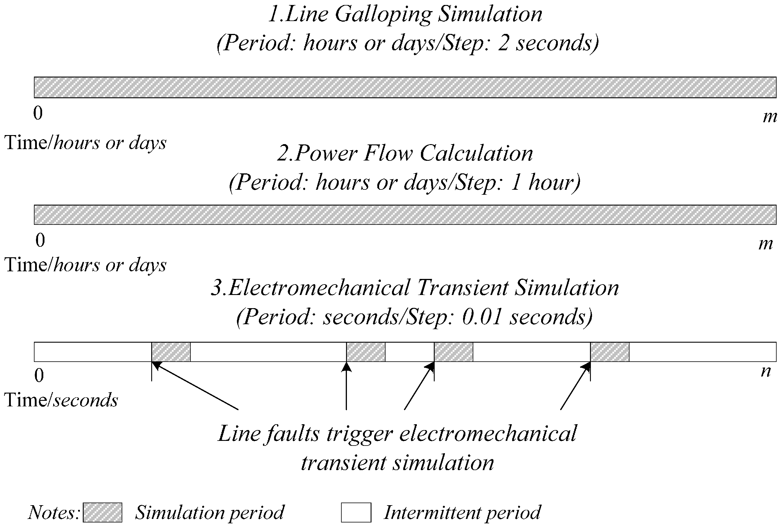
Actually, the simulation of line galloping and power systems should both be conducted throughout the entire simulation period and simultaneously. However, the wind disaster may last for several hours, which will affect the efficiency of the simulation of the power system. Therefore, the two simulation situations need to be coupled into one simulation framework as shown in Figure 4.
The process of line galloping is of long duration and low precision; however high efficiency and precision is necessary for power system simulation. Hence, line-galloping simulation is conducted throughout the entire period with the step of 2 s. When an electrical fault is triggered, power system dynamic simulation will be conducted for 10 s with the step of 0.01 s. When power system dynamic simulation ends, the result will be saved for power flow calculation. Furthermore, to consider the load fluctuation in the power grid, power flow calculation is conducted throughout the entire period with the step of 1 h. This way, the efficiency and precision of simulation can both be guaranteed. The load fluctuation data adopted in our research is extracted from a typical operation mode, as shown in Figure 5. Different load variation patterns can be adopted with different load data files. Though the results in the paper are based on the specific load variation pattern, it is easy to check the impact of load variation by changing its data file.
4.2. Relationship between Line-Galloping Amplitude and Line Fault Probability
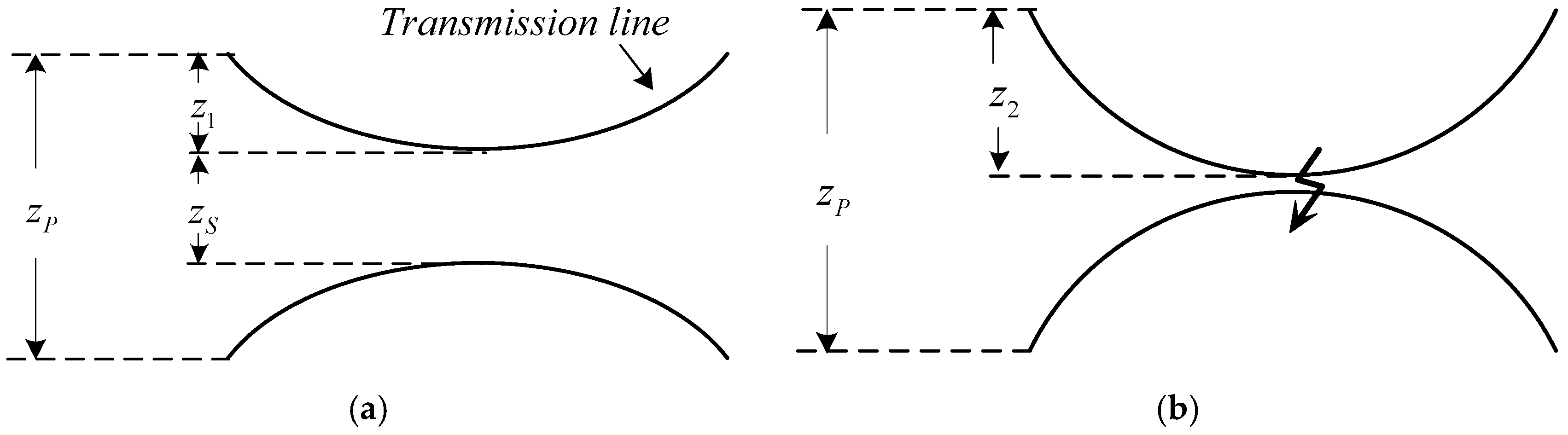
Line galloping amplitude will affect the probability of line faults. When the amplitude is small, no accidents will happen. Otherwise, when it is large enough, flashover, short circuit between phases, or other disturbances may be triggered. As shown in Figure 6, when amplitude is above z1, the failure of transmission lines begins to occur, and when it is above z2, short circuit is certain to happen.
The nature of single-phase or interphase short circuit is the breakdown of voltage. According to Pasehen’s law [20], the breakdown voltage of the medium is a function of the product of the gas pressure and the gap distance between the mediums. Firstly, gas pressure between lines is assumed as constant. Secondly, when the gap distance is large, the function curve approximates the straight line of a fixed slope. Therefore, the relationship between line-galloping amplitude and line fault probability can be assumed as linear. The relationship can be simplified and formulated as Equation (9):
where z is the amplitude of line galloping, η is the probability of line faults.
4.3. Line Fault Self-Defined Sampling
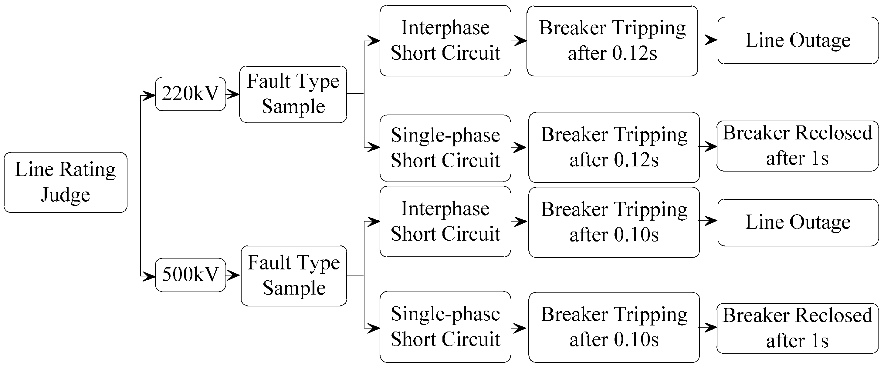
When line galloping results in line faults, interphase or single-phase short circuit may be triggered. The detailed settings are shown in Figure 7, which is based on the “Guide on Security and Stability for Power System”.
In the settings, the probability of single-phase and interphase short circuit can be defined according to the actual situation. The statistics data of a historical line-galloping event in a regional power grid is adopted in this paper.
5. Case Studies
The simulation framework is deployed based on PSS/E, and the following assumptions are made.
- The ice accretion thickness is constant during the simulation period. The shape of ice is also assumed fixed.
- Weather data are all assumed to be forecasted information, which are simulated based on actual field data.
- The accumulated mechanical harm of wind galloping on the structure of towers or other structures is neglected.
5.1. Case Descriptions
5.1.1. Grid Data
Case studies were conducted using the 23-bus model provided by PSS/E, as shown in Figure 8. In the test system, six machines and 23 nodes are all exposed to strong wind.
The parameters of transmission lines include voltage level, cross-sectional area, tensile force, line length, and so on. Taking eight of them as an example, the detailed parameters are shown in Table 1.
For transmission lines of 220 kV and 500 kV, the phase distance and safety distance are as shown in Table 2.
5.1.2. Weather Information
Many meteorological factors will affect the occurrence of line galloping, such as wind direction, wind speed, temperature, and precipitation. Under appropriate temperature and precipitation, ice accumulates on transmission lines and turns into oval ice accretion, which is easy to trigger line-galloping events. In the simulation period of this paper, it is assumed that the ice formation at a certain temperature and precipitation is constant. After the calculation of wind speed and wind direction, the wind speed perpendicular to the long axis of the icing ellipse is shown in Figure 9.
5.1.3. Simulation Settings
The simulation periods and steps of three processes are set as Table 3.
Line galloping is simulated throughout the whole period with the step of 2 s. Power flow is updated every 1 h to consider load fluctuation. Transient simulation is triggered for 10 s when line faults occur, with the step of 0.01 s. The result of current transient simulation will be the initial state of transient simulation the next time.
5.2. Simulation Results
Line galloping is an accident of high randomness, which is reflected through the probability sample module in the simulation. Thus, the results of every simulation will be different. Line galloping is a complicated process of high randomness. Even in the same meteorological environment, instances of line galloping differ from each other. Therefore, the probability statistics method based on the simulation of large numbers is adopted. With more simulations, the result will be more precise. On the other hand, the time cost will also grow. Considering both simulation accuracy and efficiency, 100 times are applied in our research. The statistic results of 100 cases are listed in Table 4.
5.2.1. Analysis of Unstable Scenarios
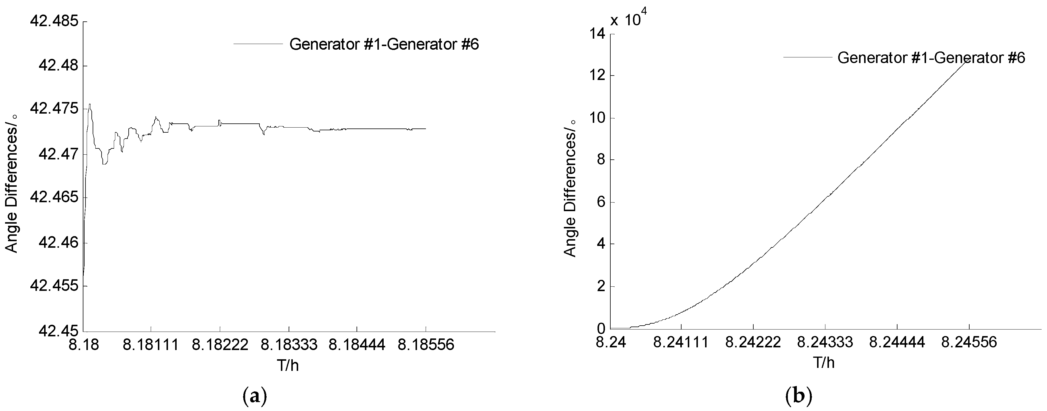
Take an unstable fault scenario as an example, as shown in Table 5.
Suffering above listed cascading faults, the biggest angle differences occurred between generator #1 and #6, as shown in Figure 10. In Fault No. 2, 5 and 9, line #9, #5 and #14 have been tripped due to interphase short circuit. Therefore, the interphase short circuit and line tripping of line #13 in Fault No. 12 result in a partial blackout of the power grid.
5.2.2. Analysis of Stable Scenarios
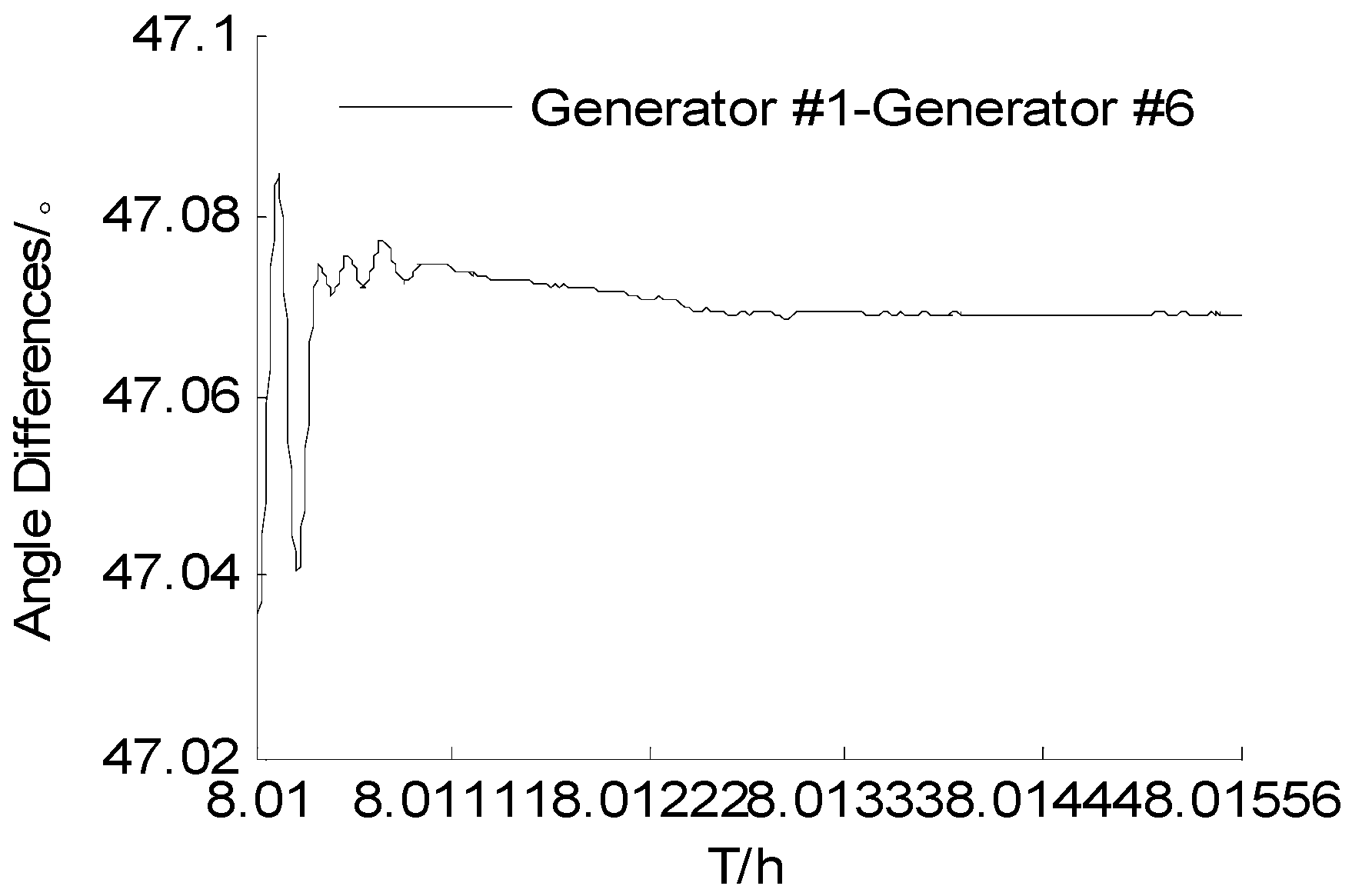
Take a stable fault scenario as an example, as listed in Table 6.
In the fault scenario, when fault No. 1 is triggered, the angle differences between generator #1 and #6 fluctuates out of the short circuit of line #1, as shown in Figure 11.
Electrical variables also change with the occurrence of line faults. Take the eight transmission lines listed in Table 1 as an example. When line #3 and #1 are broken at 8:08:24 and 8:21:00, respectively, the line current instantly falls to zero. The current of the other six transmission lines also fluctuate with the influence of single-phase short circuit and line breaking, as shown in Figure 12.
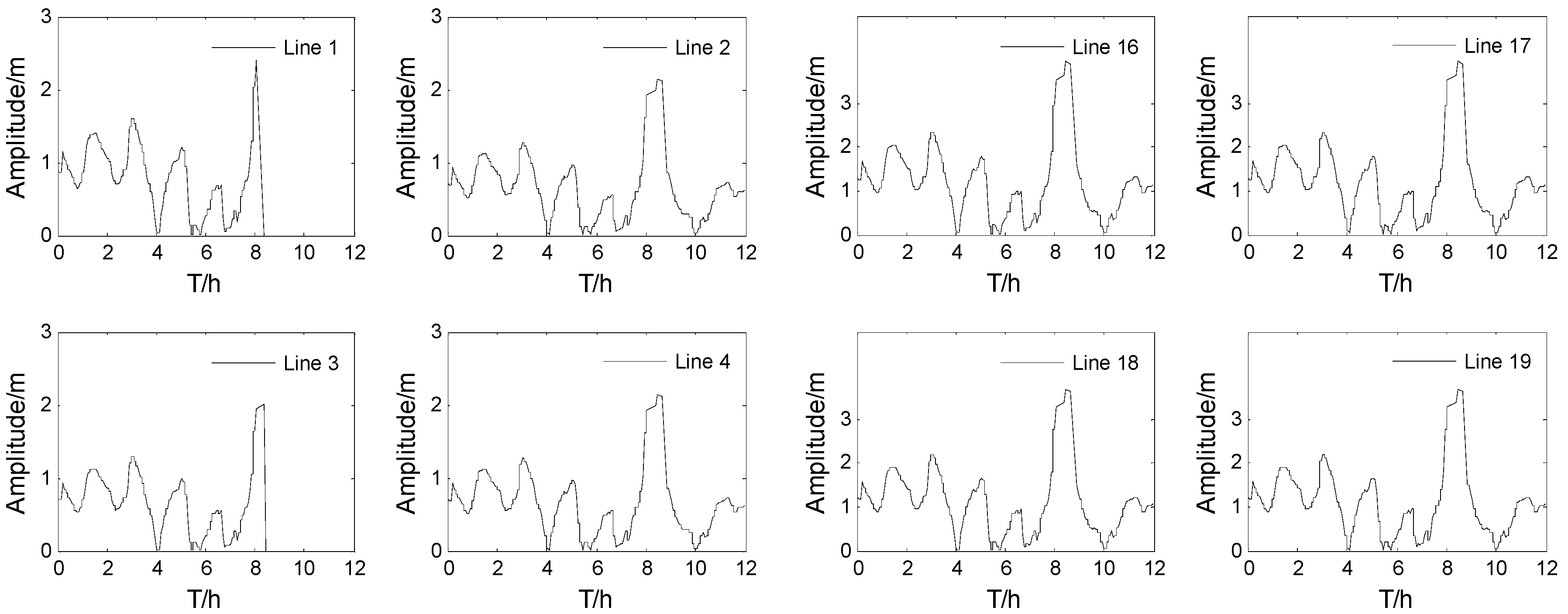
Besides electrical responses, the line-galloping dynamic process also can be acquired as shown in Figure 13. When interphase short circuit happens in some transmission lines, the corresponding line will be broken, and the amplitude turns to be zero.
5.3. Efficiency of Simulation Platform
In the simulation platform presented above, simulation efficiency is determined by the following parts:
• Calculation of line-galloping amplitude
The calculation of line-galloping amplitude is based on ambient environment, whose core problem is the solution of nonlinear algebraic equations. The calculation is carried out every two seconds, which is determined by the updating of input information.
• Sampling of line fault
Based on the relationship between the amplitude of the line and the fault type, the fault is sampled to determine whether the fault occurs or not. Fault type and detailed settings differ with the voltage level of transmission lines. The sampling is triggered when a short circuit fault occurs.
• Power flow calculation
Power flow is calculated to update the load data every hour.
• Electromechanical transient simulation
When line faults occur, electromechanical transient simulation is triggered and lasts for 20 s. The times of the execution of this part depend on the times of occurrence of faults.
Eight cases were tested in a desktop computer with a CPU of four cores (3.20 GHz) to illustrate the efficiency of our simulation platform. The results are shown as Table 7.
According to simulation results, a line galloping of 10 h can be simulated in several minutes. When the case is more complex, simulation time will be longer. However, the high efficiency of simulation can ensure the application of this simulation platform, which can provide appropriate advice and guides for operators.
6. Discussion
The hybrid simulation framework of a power system considering line galloping is constructed to simulate the random clustered, long-timescale cascading faults caused by strong wind weather conditions. The impact mechanism and dynamic processes between power systems and meteorological systems are revealed. An extended software package for PSS/E is developed to carry out the hybrid simulation. Based on this platform, two dynamic processes of power systems and meteorological systems with different time scales are combined into one simulation and can be solved efficiently. The power system simulation concept is extended by considering the meteorological system.
The distributed computation is a good approach to further improve simulation efficiency, which will be carried out in the future. The simulation processes last for the whole period in which every module interacts with each other. However, simulations are conducted for large numbers of times repeatedly with same input information and parameter settings in our framework. Therefore, the simulation can be carried out independently with different computers. The sum results of the simulations will be obtained with distributed computation. The simulation approach proposed in the paper is mainly used for early warning of non-secure situations during the coming of extreme weather. With forecasted extreme weather information, the risk of power grid blackout can be obtained based on the proposed simulation platform. Dispatchers can adjust the operation mode of power grid to reduce losses in the instances of such weather events.
Acknowledgments
This work is jointly supported by National Natural Science Foundation of China (No: 51477092), State Grid Corporation of China (No. XT71-16-043) and National Key Research and Development Program of China (2017YFB0902802).
Author Contributions
Hengxu Zhang conceived the main idea and provided guidance for the study. Lizheng Chen performed the simulations, analyzed the results and wrote the manuscript. Changgang Li and Huadong Sun performed some case studies and polished the manuscript.
Conflicts of Interest
The authors declare no conflict of interest.
References
- Kermani, M.; Farzaneh, M.; Kollar, L.E. The effects of wind induced conductor motion on accreted atmospheric ice. IEEE Trans. Power Deliv. 2013, 28, 540–548. [Google Scholar] [CrossRef]
- Hume, M. Environment Canada Warns More Bad Weather Coming to Metro Vancouver. Available online: http://www.theglobeandmail.com/news/british-columbia/windstorm-causes-hundreds-of-thousands-of-power-outages-in-southwest-bc/article26156947/ (accessed on 29 August 2015).
- Zhu, K.J.; Liu, B.; Niu, H.J.; Li, J.H. Statistical analysis and research on galloping characteristics and damage for iced conductors of transmission lines in China. In Proceedings of the 2010 International Conference on Power System Technology, Hangzhou, China, 24–28 October 2010. [Google Scholar]
- Den Hartog, J.P. Transmission line vibration due to sleet. IEEE Trans. Am. Inst. Electr. Eng. 1932, 51, 1074–1076. [Google Scholar] [CrossRef]
- Abdul, B.; Anca, D.H.; Mufit, A.; Poul, E.S.; Mette, G. Compensating active power imbalances in power system with large-scale wind power penetration. J. Mod. Power Syst. Clean Energy 2016, 4, 229–237. [Google Scholar]
- Guo, Y.L.; Li, G.X.; You, C.Y. Transmission Lines Galloping; China Electric Power Press: Beijing, China, 2003. [Google Scholar]
- Nigol, O.; Buchan, P.G. Conductor galloping: Part I—Den Hartog mechanism. IEEE Trans. Power Appar. Syst. 1981, 100, 699–707. [Google Scholar] [CrossRef]
- Nigol, O.; Buchan, P.G. Conductor galloping: Part II—Torsional mechanism. IEEE Trans. Power Appar. Syst. 1981, 100, 708–720. [Google Scholar] [CrossRef]
- Hu, J.; Yan, B.; Zhou, S.; Zhang, H. Numerical Investigation on Galloping of Iced Quad Bundle Conductors. IEEE Trans. Power Deliv. 2012, 27, 784–792. [Google Scholar] [CrossRef]
- Borna, A.; Habashi, W.G.; McClure, G.; Nadarajah, S.K. Numerical modeling of ice accretion effects on galloping of transmission line conductors. In Proceedings of the 9th International Symposium on Cable Dynamics, Shanghai, China, 18–20 October 2011. [Google Scholar]
- Yu, P.; Desai, Y.M.; Shah, A.H.; Popplewell, N. Three-degree-of freedom model for galloping. Part II: Solutions. J. Eng. Mech. 1993, 119, 2426–2448. [Google Scholar] [CrossRef]
- Diana, G.; Belloli, M.; Giappino, S.; Mazzola, L.; Manenti, A.; Muggiasca, S.; Zuin, A. A numerical approach to reproduce subspan oscillation and comparison with experimental data. IEEE Trans. Power Deliv. 2014, 29, 1311–1317. [Google Scholar] [CrossRef]
- Greenwood, D.M.; Ingram, G.L.; Taylor, P.C. Applying wind simulations for planning and operation of real-time thermal ratings. IEEE Trans. Smart Grid 2017, 8, 537–547. [Google Scholar] [CrossRef] [Green Version]
- Jain, H.; Parchure, A.; Broadwater, R.P. Three-Phase Dynamic Simulation of Power Systems Using Combined Transmission and Distribution System Models. IEEE Trans. Power Syst. 2016, 31, 4517–4524. [Google Scholar] [CrossRef]
- Dehghanian, P.; Kezunovic, M. Probabilistic Decision Making for the Bulk Power System Optimal Topology Control. IEEE Trans. Smart Grid 2016, 7, 2017–2081. [Google Scholar] [CrossRef]
- Hu, B.; Wang, H.; Yao, S. Optimal economic operation of isolated community micro-grid incorporating temperature controlling devices. Prot. Control Mod. Power Syst. 2017, 2, 6. [Google Scholar] [CrossRef]
- Chen, L.; Zhang, H.; Wu, Q.; Terzija, V. A numerical approach for hybrid simulation of power system dynamics considering extreme icing events. IEEE Trans. Smart Grid 2017, in press. [Google Scholar] [CrossRef]
- Sun, Q.; Shi, L.; Ni, Y.; Si, D.; Zhu, J. An enhanced cascading failure model integrating data mining technique. Prot. Control Mod. Power Syst. 2017, 2, 5. [Google Scholar] [CrossRef]
- Abdel-Rohman, M.; Spencer, B.F. Control of wind-induced nonlinear oscillations in suspended conductors. Nonlinear Dyn. 2004, 37, 341–355. [Google Scholar] [CrossRef]
- Mellinger, A.; Mellinger, O. Breakdown threshold of dielectric barrier discharges in ferroelectrets: Where paschen’s law fails. IEEE Trans. Dielectr. Electr. Insul. 2011, 18, 43–48. [Google Scholar] [CrossRef]
Figure 1.
Simulation framework of faults caused by line galloping.
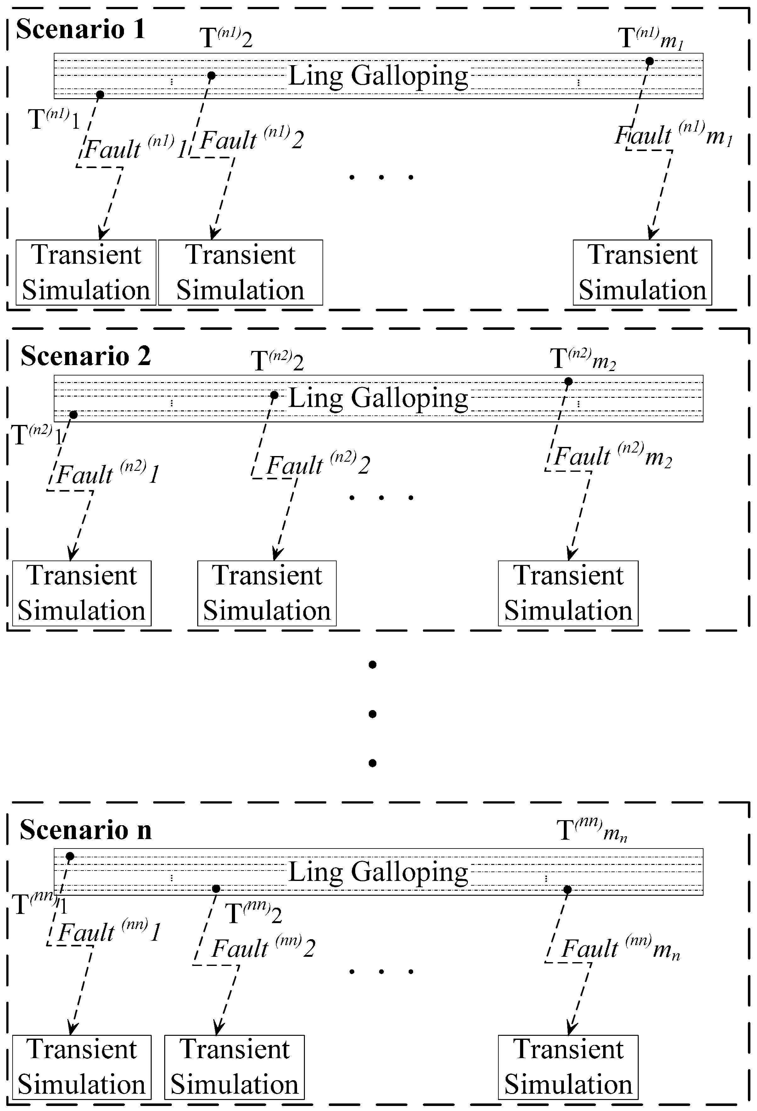
Figure 2.
Simulation Process of Fault Scenarios Caused by Line Galloping.
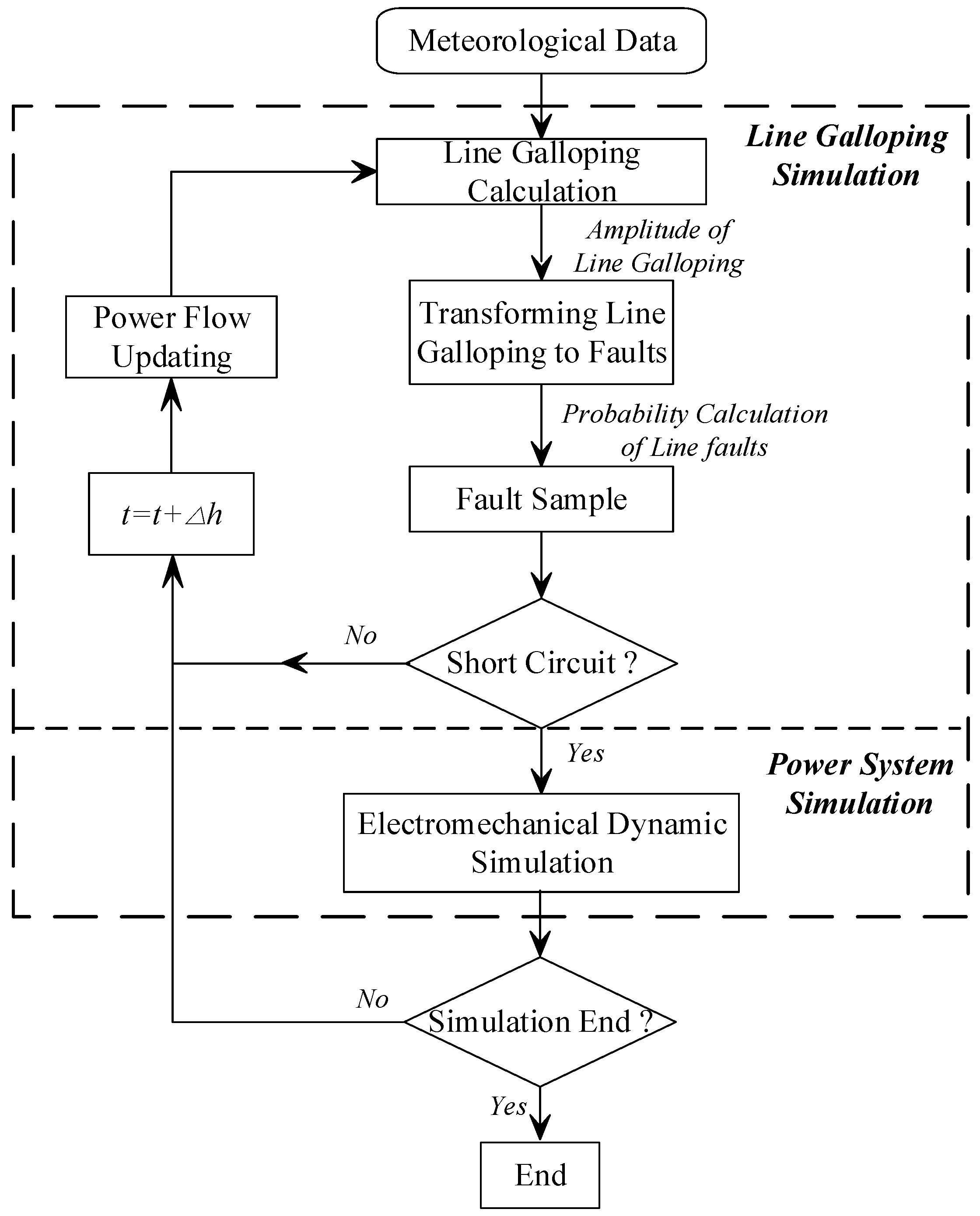
Figure 3.
Information interface of power system and line galloping.

Figure 4.
Timescales of the power system and meteorological systems.

Figure 5.
Load fluctuation of power grid.
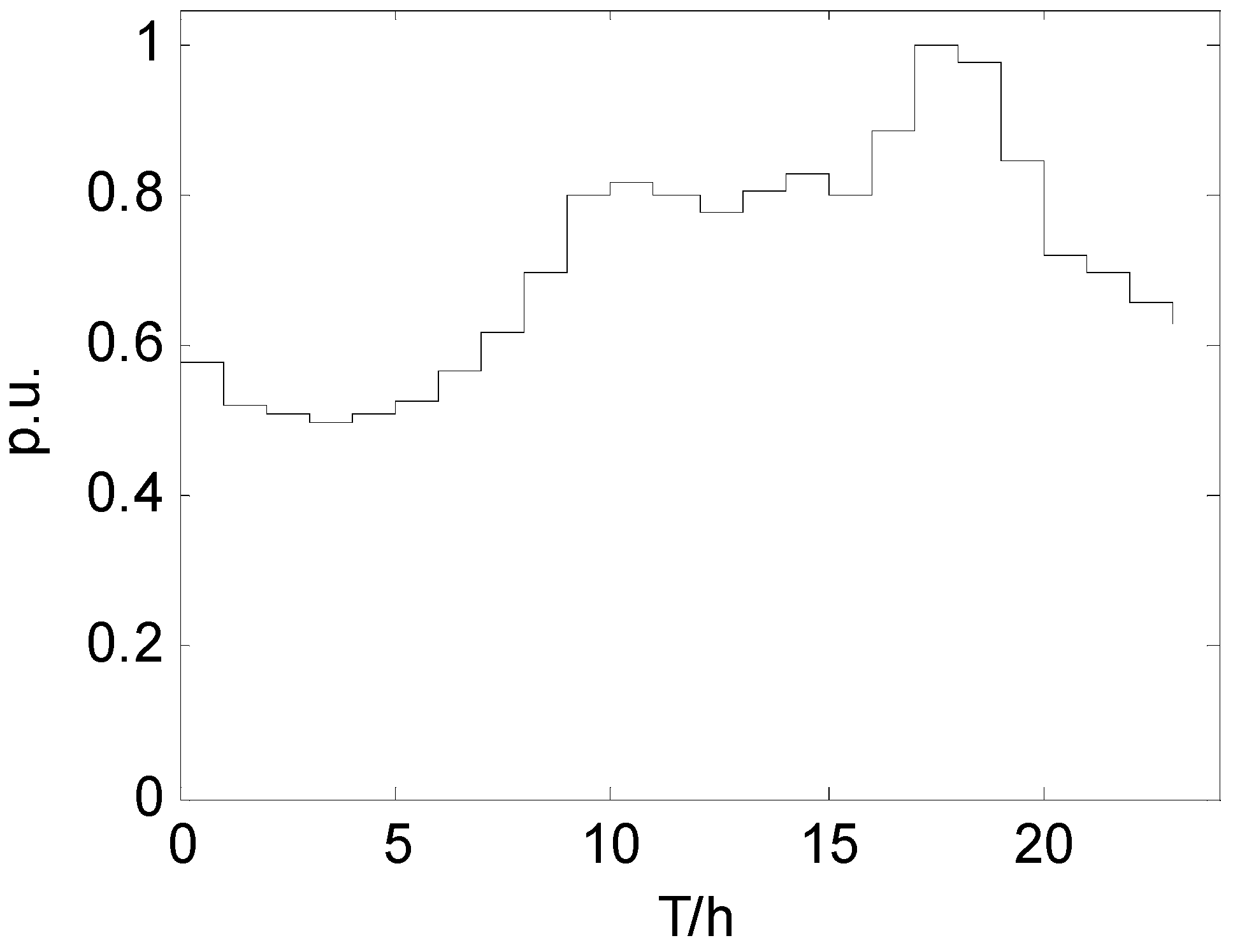
Figure 6.
Line-galloping amplitude relationship. (a) Small line-galloping amplitude; (b) Large line-galloping amplitude.
Figure 6.
Line-galloping amplitude relationship. (a) Small line-galloping amplitude; (b) Large line-galloping amplitude.

Figure 7.
Settings of electrical fault type.

Figure 8.
Case of 23 nodes of power system simulator/engineering (PSS/E).
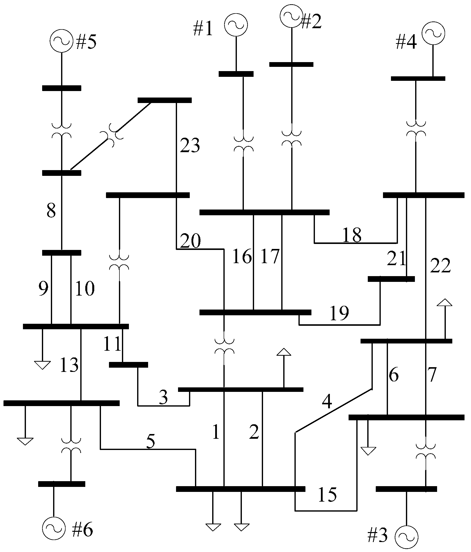
Figure 9.
Wind speed perpendicular to the long axis of the icing ellipse.
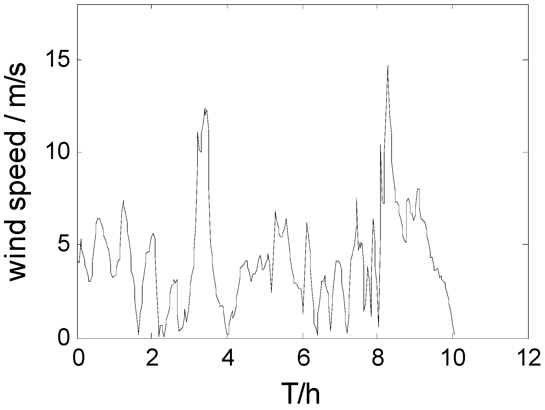
Figure 10.
Angle differences between generator #1 and #6. (a) Fault No. 11; (b) Fault No. 12.

Figure 11.
Angle differences between generator #1 and #6.

Figure 12.
Current of transmission lines.
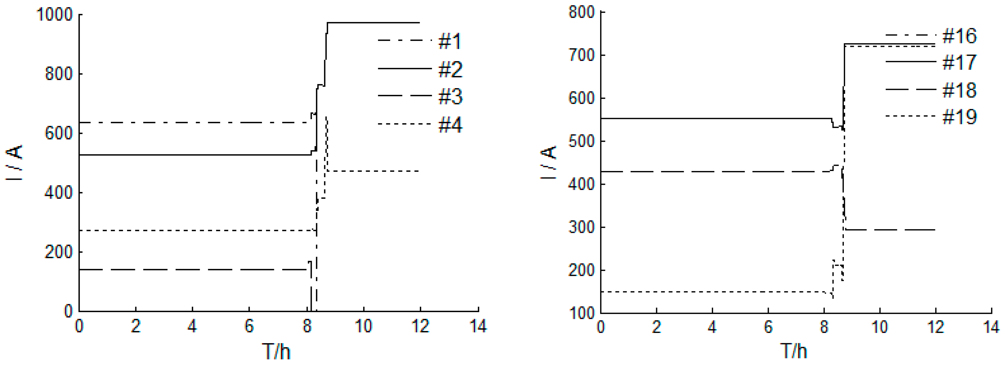
Figure 13.
Amplitudes of line galloping.

Table 1.
Parameters of eight transmission lines.
| No. | Voltage Level/kV | Cross Sectional Area/mm2 | Tensile Force/kN | Length/(m) |
|---|---|---|---|---|
| 1 | 220 | 121.21 | 19,420 | 250 |
| 2 | 220 | 121.21 | 19,420 | 250 |
| 3 | 220 | 121.21 | 19,420 | 200 |
| 4 | 220 | 121.21 | 19,420 | 200 |
| 16 | 500 | 397.83 | 61,150 | 800 |
| 17 | 500 | 397.83 | 61,150 | 800 |
| 18 | 500 | 397.83 | 61,150 | 750 |
| 19 | 500 | 397.83 | 61,150 | 750 |
Table 2.
Numerical distance of transmission lines.
| Voltage Level (kV) | Phase Distance (zp)/m | Safety Distance (zs)/m | z1/m | z2/m |
|---|---|---|---|---|
| 220 | 6 | 3 | 1.5 | 3 |
| 500 | 11 | 5 | 3 | 5.5 |
Table 3.
Settings of simulation period and step.
| Simulation Process | Period | Step |
|---|---|---|
| Line Galloping | 10 h | 2 s |
| Power Flow | 10 h | 1 h |
| Transient Simulation | 10 s | 0.01 s |
Table 4.
Statistics of simulation results.
| Scenario State | Times |
|---|---|
| Stable | 89 |
| Unstable | 11 |
Table 5.
Detailed process of unstable fault scene.
| Fault No. | Fault Time | Fault Lines | Fault Type | Description |
|---|---|---|---|---|
| 1 | 7:58:48 | Line #5 | single-phase short circuit | breaker reclosed after 0.12 s |
| 2 | 8:00:00 | Line #9 | interphase short circuit | line breaking after 0.12 s |
| 3 | 8:01:48 | Line #15 | single-phase short circuit | breaker reclosed after 0.12 s |
| 4 | 8:04:48 | Line #3 | single-phase short circuit | breaker reclosed after 0.12 s |
| 5 | 8:05:24 | Line #5 | interphase short circuit | line breaking after 0.12 s |
| 6 | 8:06:00 | Line #7 | single-phase short circuit | breaker reclosed after 0.12 s |
| 7 | 8:07:12 | Line #11 | single-phase short circuit | breaker reclosed after 0.12 s |
| 8 | 8:07:48 | Line #13 | single-phase short circuit | breaker reclosed after 0.12 s |
| 9 | 8:08:24 | Line #14 | interphase short circuit | line breaking after 0.12 s |
| 10 | 8:08:24 | Line #15 | single-phase short circuit | breaker reclosed after 0.12 s |
| 11 | 8:10:48 | Line #1 | single-phase short circuit | breaker reclosed after 0.12 s |
| 12 | 8:14:24 | Line #13 | interphase short circuit | line breaking after 0.12 s |
Table 6.
Detailed process of stable fault scene.
| Fault No. | Fault Time | Fault Lines | Fault Type | Description |
|---|---|---|---|---|
| 1 | 8:00:36 | Line #1 | single phase short circuit | breaker reclosed after 0.12 s |
| 2 | 8:01:12 | Line #3 | single-phase short circuit | breaker reclosed after 0.12 s |
| 3 | 8:01:48 | Line #5 | single-phase short circuit | breaker reclosed after 0.12 s |
| 4 | 8:02:24 | Line #7 | single-phase short circuit | breaker reclosed after 0.12 s |
| 5 | 8:03:00 | Line #9 | interphase short circuit | line breaking after 0.12 s |
| 6 | 8:03:48 | Line #10 | single-phase short circuit | breaker reclosed after 0.12 s |
| 7 | 8:03:48 | Line #11 | single-phase short circuit | breaker reclosed after 0.12 s |
| 8 | 8:04:48 | Line #15 | single-phase short circuit | breaker reclosed after 0.12 s |
| 9 | 8:07:48 | Line #1 | single-phase short circuit | breaker reclosed after 0.12 s |
| 10 | 8:08:24 | Line #3 | interphase short circuit | line breaking after 0.12 s |
| 11 | 8:10:48 | Line #12 | single-phase short circuit | breaker reclosed after 0.12 s |
| 12 | 8:13:48 | Line #22 | single-phase short circuit | breaker reclosed after 0.10 s |
| 13 | 8:21:00 | Line #1 | interphase short circuit | line breaking after 0.12 s |
| 14 | 8:33:00 | Line #19 | single-phase short circuit | breaker reclosed after 0.10 s |
| 15 | 8:36:36 | Line #7 | single-phase short circuit | breaker reclosed after 0.12 s |
| 16 | 8:40:48 | Line #21 | interphase short circuit | line breaking after 0.10 s |
| 17 | 8:45:36 | Line #14 | single-phase short circuit | breaker reclosed after 0.12 s |
Table 7.
Statistics of simulation time.
| Scenario No. | Scenario State | Time Cost |
|---|---|---|
| 1 | stable | 80 s |
| 2 | stable | 101 s |
| 3 | stable | 98 s |
| 4 | stable | 123 s |
| 5 | stable | 86 s |
| 6 | stable | 90 s |
| 7 | stable | 120 s |
| 8 | stable | 116 s |
| 9 | unstable | 182 s |
| 10 | stable | 86 s |
© 2017 by the authors. Licensee MDPI, Basel, Switzerland. This article is an open access article distributed under the terms and conditions of the Creative Commons Attribution (CC BY) license (http://creativecommons.org/licenses/by/4.0/).
Share and Cite
MDPI and ACS Style
Chen, L.; Zhang, H.; Li, C.; Sun, H. Modeling and Simulating Long-Timescale Cascading Faults in Power Systems Caused by Line-Galloping Events. Energies 2017, 10, 1301. https://doi.org/10.3390/en10091301
AMA Style
Chen L, Zhang H, Li C, Sun H. Modeling and Simulating Long-Timescale Cascading Faults in Power Systems Caused by Line-Galloping Events. Energies. 2017; 10(9):1301. https://doi.org/10.3390/en10091301
Chicago/Turabian StyleChen, Lizheng, Hengxu Zhang, Changgang Li, and Huadong Sun. 2017. "Modeling and Simulating Long-Timescale Cascading Faults in Power Systems Caused by Line-Galloping Events" Energies 10, no. 9: 1301. https://doi.org/10.3390/en10091301
Note that from the first issue of 2016, this journal uses article numbers instead of page numbers. See further details here.