Economic Valuation of Low-Load Operation with Auxiliary Firing of Coal-Fired Units

State Key Laboratory of Advanced Electromagnetic Engineering and Technology, Huazhong University of Science and Technology, No.1037, Luoyu Road, 430074 Wuhan, China
*
Author to whom correspondence should be addressed.
Energies 2017, 10(9), 1317; https://doi.org/10.3390/en10091317
Submission received: 6 August 2017
/
Revised: 28 August 2017
/
Accepted: 29 August 2017
/
Published: 1 September 2017
(This article belongs to the Section F: Electrical Engineering)
Abstract
:It is often claimed that coal-fired units are highly inflexible to accommodate variable renewable energy. However, a recently published report illustrates that making existing coal-fired units more flexible is both technically and economically feasible. Auxiliary firing is an effective and promising measure for coal-fired units to reduce their minimum loads and thus augment their flexibility. To implement the economic valuation of low-load operation with auxiliary firing (LLOAF) of coal-fired units, we improve the traditional fuel cost model to express the operating costs of LLOAF and present the economic criterion and economic index to assess the economics of LLOAF for a single coal-fired unit. Moreover, we investigate the economic value of LLOAF in the power system operation via day-ahead unit commitment problem and analyze the impacts on the scheduling results from unit commitment policies and from extra auxiliary fuel costs. Numerical simulations show that with the reduction of the extra auxiliary fuel costs LLOAF of coal-fired units can remarkably decrease the total operating costs of the power system. Some further conclusions are finally drawn.
1. Introduction
Renewable energy is recognized as central to achieving global climate and sustainability objectives. Variable renewable energy (VRE), especially wind power and solar power, is playing an increasingly significant role to reach these objectives [1]. According to the 2030 renewable energy roadmap published by the International Renewable Energy Agency (IRENA), half of Germany’s total power generation is expected to come from VRE, and the share of VRE in the U.S. may reach 30% [2,3]. However, VRE is inherently intermittent with uncertain characteristics that pose a formidable challenge to the operation of power systems. To accommodate the increasing share of VRE, it is crucial to improve the operational flexibility of power systems [4]. This recommendation has gained strong support from many system operators and regulatory commissions across the world. Some U.S. system operators have introduced a specific flexible ramping product (CAISO [5], MISO [6]) to produce sufficient price incentives for the eligible resources to provide their operational flexibility. Chinese National Energy Administration has lately started the ancillary services market reform pilot program in the Northeast power system to encourage more power plants to provide operational flexibility [7].
Power systems previously depended largely on coal-fired power plants to generate electricity. It is often claimed that existing coal-fired power plants are highly inflexible to cope with VRE. As a result, there is a rising level of VRE curtailment in some power systems. However, a recently published report [8] shows that making existing coal-fired power plants more flexible is both technically and economically feasible. The report takes Germany and Denmark as examples of successful modifications of coal-fired power plants. Both countries now operate coal-fired power plants, which were originally highly inflexible, almost as flexibly as gas-fired plants. On the one hand, augmenting the flexibility of coal-fired power plants represents a major strategy to effectively integrate large shares of VRE into the power systems characterized by few other flexibility options and very high shares of existing inflexible power plants, for instance in China and Poland. This strategy has gained strong support from recently published Chinese energy policy [9,10]. On the other hand, even for other power systems with more flexibility options, conventional power plants may have to provide more flexible services in the future to accommodate the increasing shares of VRE. Augmenting the operational flexibility allows them to adapt better the future electricity market competition.
The operational flexibility of a coal-fired unit can be described as its ability to adjust the net power fed into the grid, its overall bandwidth of operation, and the time required to attain stable operation when starting up from a standstill [8]. The key parameters characterizing the flexibility of a coal-fired unit include minimum load, start-up time and ramp rate. The minimum load is deemed to be the most crucial flexibility parameter. Reducing minimum load extends the power output range of coal-fired units and avoids expensive startups and shutdowns when power demand is low. From a system standpoint, it allows a great share of VRE by avoiding potential curtailment. Moreover, it allows the units to provide more ancillary services relative to the start-stop cycling mode, including regulation, load following, and other operating reserves, and thus makes the units more competitive in the electricity market.
Reducing minimum load is subject to many technical limitations, including fire stability, flame control, ignition, and unburned coal. Several retrofit options exist for overcoming many of these limitations, such as indirect firing, switching from two-mill to single-mill operation, thermal energy storage, and auxiliary firing [8]. As the use of lower rank coals such as lignite is gaining increasing importance worldwide, fire stability is becoming more crucial to reducing minimum load [11]. Auxiliary firing is an effective and mature measure to stabilize the fire in the boiler and thus can reduce the minimum load. It improves the fire stability in the extreme low-load operation by combusting auxiliary fuels, such as oil or gas, in addition to the pulverized coal. But combusting expensive oil or gas may largely impair the economics of extreme low-load operation. Micro-oil [12] and oxy-fuel combustion [13] are available technologies that reduce the consumption of auxiliary fuels. Further, indirect firing of dried coals can also serve as auxiliary firing at extremely low loads to largely reduce the consumption of expensive auxiliary fuels such as fuel oil and natural gas [14]. Besides, there are some other auxiliary firing technologies that provide us more alternatives to reduce the costs of auxiliary firing, such as plasma igniters or electrical preheating of the burner’s fuel nozzle.
This paper evaluates the economic value of low-load operation with auxiliary firing (LLOAF) of coal-fired units. The evaluation uses the general expression to represent the costs and benefits incurred by LLOAF and thus applies to many auxiliary firing technologies. For the convenience of description, the costs incurred by auxiliary firing are described as auxiliary fuel costs. The price of auxiliary fuel is assumed to be higher than that of raw fuel coal in this paper.
On the one hand, LLOAF increases the operating costs of coal-fired units because the auxiliary fuel price is higher than the raw coal price and LLOAF leads to lower efficiency relative to nominal load operation. On the other hand, LLOAF increases the operational flexibility of coal-fired units and allows the units to get more revenues by providing flexibility services. From the perspective of the owner of the units, LLOAF is economical only when its revenue increases can compensate its cost increases.
Accurately modeling the operating costs is the basis for the economic valuation of LLOAF of coal-fired units. The operating costs of coal-fired units are usually depicted by fuel cost models in the power system operation formulations [15,16,17]. These models assume that the fuel composition at different load levels is consistent, and thus, the fuel cost models can be expressed as continuous functions such as linear functions, convex quadratic functions, non-convex continuous functions [18,19]. However, the fuel composition changes in the LLOAF, in which fuel coal is combusted together with auxiliary fuel. The mixed combustion leads to the mutation in the fuel cost curve at the load level at which auxiliary fuel begins to inject into the boiler. Thus, the traditional continuous functions no longer apply to expressing the operating costs of LLOAF. This paper extends the traditional fuel cost model to express the operating costs of LLOAF. The improved fuel cost model is expressed as the set of mixed-integer linear constraints, which facilitates the modeling and solving of various power system operation problems concerning LLOAF of coal-fired units.
The revenues of LLOAF come from the benefits brought by its increased flexibility capacity. We first express the revenues of LLOAF by promoting the use of VRE to reduce the fuel costs. Based on the above-mentioned improved fuel cost model, we present an economic criterion to assess whether LLOAF is economical for a single coal-fired unit. This criterion provides the precondition for the coal-fired units to promote the use of VRE through LLOAF. According to this criterion, we further analyze the key factors affecting the economics of LLOAF and provide some reference for the auxiliary firing retrofit of coal-fired units accordingly.
To fully tap the flexibility potential of coal-fired power plants, it is crucial to give incentives for the flexible operation of coal-fired power plants through adjusting electricity market design. But before remunerating flexibility, we should evaluate the economic value of flexibility in the power system operation. The economic evaluation of LLOAF is implemented in the day-ahead unit commitment (UC) problem in this paper. The day-ahead UC is the short-term planning process that is commonly used to schedule the units at the minimum costs within all the technical limits [20]. Different UC policies, including the stochastic and deterministic ones, are tested in this paper to study their impact on the scheduling results. In the UC problem, the economic value of LLOAF includes not only its impact on the use of VRE but also other benefits in the scheduling strategy.
The remainder of this paper is organized as follows: the fuel cost model considering LLOAF is presented in Section 2. Section 3 presents the economic criterion and economic index for LLOAF and analyzes the related factors that affect the economics of LLOAF. Section 4 describes the different UC formulations that are implemented. Numerical simulations are provided in Section 5. Finally, Section 6 summarizes this work.
2. Fuel Cost Model Considering LLOAF
At present, the fuel cost model of coal-fired units only considers a single type of fuel input and can thus be expressed as the product of the input-output function and the fuel price. The input-output function is used to measure the heat energy (the input) required per hour to maintain various levels of generation (the output) [18,21]. The heat energy is always measured in tons of coal for coal-fired units. However, when a coal-fired unit is in the LLOAF, the fuel input includes both pulverized coal and auxiliary fuel, so the traditional fuel cost model is no longer applicable.
Assuming that the minimum load of a coal-fired unit without auxiliary firing is and the minimum load with auxiliary firing is . The load of a unit can also be called as the power output of the unit to the power grids, the two terminologies are identical and used equally in this paper. When the power output is not less than , the traditional fuel cost model is applicable. When the power output is less than but not less than , the unit is in the LLOAF, the traditional fuel cost model should be revised to consider the change of the fuel composition.
Assuming that the power output is , according to the input-output function the total fuel consumption per hour is measured in tons of coal equivalent (TCE), in which the amount of auxiliary fuel measured in TCE is ; then, the amount of coal fuel is . Assuming that the price of fuel coal measured in TCE is and the price of auxiliary fuel measured in TCE is , then the fuel costs for the power output P are expressed as Equation (1). It is better to transform Equation (1) into Equation (2), in which replaces , because measures the combustion characteristics of the coal-fired unit and corresponds to the input-output function.
The first term on the right side of Equation (2) is identical to the traditional fuel cost function and can be regarded as the fuel cost measured in the coal price (abbreviated as coal fuel costs hereinafter). The second term represents the additional fuel costs incurred by the auxiliary fuel (abbreviated as extra auxiliary fuel costs, EACs). For modeling convenience, the amount of auxiliary fuel is approximated as a constant for a given unit, so that EACs can be independent of the power output of the unit.
In the entire power output range from 0 to the rated capacity, the complete fuel cost model of a coal-fired unit can be expressed as follows:
where represents the rated capacity.
However, Equation (3) is a piecewise discontinuous function, which is not conducive to the modeling of the problems concerning LLOAF. Equation (3) can be rewritten as Equation (4) by introducing the binary variable . In Equation (4), the fuel cost model is expressed in a uniform form, where the first term is identical to the traditional fuel cost function and the second term can be considered separately. The variable is used to represent the state of LLOAF. It is equal to 1 when the unit is in the LLOAF, and 0 otherwise. The values of the binary variable are shown as Equation (5):
where is the traditional fuel cost function, the constant represents the EACs, and the variable represents the commitment of the unit.
Further, Equation (5) can be expressed as the following inequality constraints. Constraints (6)–(8) correspond to the three cases of Equation (5). Consequently, the fuel cost model is expressed as the set of mixed-integer linear constraints, which allows the operation problems concerning LLOAF to be solved directly by the commercially available software:
where is an arbitrary positive constant and is introduced to make the constraint (8) satisfy the situation .
3. Economic Criterion for LLOAF and Related Factors
LLOAF can augment the flexibility of coal-fired units and thus allows the units to obtain more revenues by providing more flexible services. In this section, we assume that the increased flexible capacity from LLOAF is used to promote the use of VRE and the revenues of LLOAF come from the fuel cost savings by substituting VRE for the energy produced by coal-fired units. For simplicity, the production costs of VRE are assumed to be negligible in this paper. The increased flexible capacity of LLOAF can also be used for other purposes, however, which are not the main content of this section.
The precondition of LLOAF for a unit is that its revenues can compensate its increased costs. Based on the above fuel cost model considering LLOAF, we present the economic criterion to judge whether a unit has the possibility to meet this precondition.
3.1. Economic Criterion and Economic Index for LLOAF
The fuel cost function of a coal-fired unit considering LLOAF is shown in Figure 1, which shows that there is a mutation in the fuel cost curve at point . As seen in Figure 1, we assume that there is a point in the LLOAF where its fuel costs are equal to the fuel costs at point . The point is referred to the equilibrium point hereinafter. When , LLOAF allows using more VRE with the amount of , however, the fuel costs at are higher than the fuel costs at , operating the unit at is less economical than operating the unit at and abandoning such amount of VRE. In such a case, promoting the use of VRE by LLOAF cannot compensate the increased costs of LLOAF, so LLOAF at is not an economical choice. When , the fuel costs at are lower than the fuel costs at , using more VRE through LLOAF can reduce the fuel costs. In such a case, LLOAF at is an economical choice.
However, if a unit has the characteristic , its equilibrium point is on the left extension of its fuel cost curve, i.e., . In such a case, the fuel costs of the unit in the LLOAF are invariably higher than its fuel costs at , so promoting the use of VRE by LLOAF fails to compensate the increased costs of LLOAF for the unit. Theoretically, such a unit is not suitable for LLOAF. Therefore, we regard the condition or as the economic criterion for LLOAF. Only in line with this economic criterion, a unit has the possibility to bring economic benefits to the power systems by LLOAF that allows using more VRE to reduce the fuel costs. This criterion applies to any situation that involves the power outputs from VRE because when a unit cannot meet this economic criterion LLOAF is less economical than avoiding the LLOAF and abandoning the VRE.
The economic criterion provides the precondition for the units to adopt the LLOAF mode, we further present the economic index to evaluate the economics of the unit in the LLOAF. When this index is less than zero, it indicates that the unit violates the economic criterion for LLOAF. When this index is positive, the larger the index is, the larger the range of LLOAF is, and therefore, the unit has better economics in the LLOAF.
3.2. LLOAF Related Factors
To evaluate the factors affecting the economic criterion, the amount of auxiliary fuel is expressed as the function of the amount of total fuel consumption at , shown as Equation (9); then, the fuel costs at can be expressed as Equation (10). Further, the economic criterion for LLOAF can be rewritten as Equation (11):
where represents the proportion of heat produced by auxiliary fuel in the total heat load (abbreviated as heat load proportion of auxiliary fuel hereinafter).
As shown in Equation (11), the factors affecting the economics of LLOAF include the heat load proportion of auxiliary fuel , the relative fuel prices , and the ratio between the fuel consumptions for the minimum loads with and without auxiliary firing (abbreviated as fuel consumption ratio hereinafter). The heat load proportion of auxiliary fuel can be reduced by improving the combustion technology, which thus can improve the economics of LLOAF. The relative fuel prices are mainly affected by market factors and auxiliary firing technologies, and the lower auxiliary fuel price will be favorable for LLOAF. The lower the fuel consumption ratio can also benefit the economics of LLOAF.
As the relative fuel prices may undergo large fluctuations in the long term, some coal-fired units may face the risk of violating the economic criterion for LLOAF. Whereas the fuel consumption ratio depends on the inherent characteristics of the unit, from the long-term planning perspective, coal-fired units with smaller fuel consumption ratios can better accommodate the uncertainty caused by the relative fuel prices. The factors affecting the fuel consumption ratio are further analyzed in the next subsection.
3.3. Analysis of the Fuel Consumption Ratio
The fuel consumption ratio is related to the input-output function of a coal-fired unit, which is commonly expressed as a linear function or a quadratic function according to the precision requirements. To facilitate the analysis, the input-output function is expressed as a linear function [22], shown as (12). Then, the fuel consumption ratio can be expressed as Equation (15), where the power outputs and are expressed in the form of load rates, i.e., the ratios relative to the rated capacity, shown as Equations (13) and (14):
where and represent the slope and intercept of the linear input-output function; and represent the load rates corresponding to the minimum loads with and without auxiliary firing.
As shown in Equation (15), the fuel consumption ratio is mainly affected by , , and the ratio . According to the empirical data of a variety of coal-fired units with different capacities, the ratio is less than 1/4 of . Therefore, the ratio can be recognized as the leading factor that affects the fuel consumption ratio.
The parameter is already known for a coal-fired unit, however, should be estimated before the retrofit of the unit. According to the above analysis, accurate estimation of the parameter contributes to prejudging the economic criterion for LLOAF. The unit with lower ratio has the larger probability to satisfy the economic criterion for LLOAF and is more suitable for auxiliary firing retrofit. Accordingly, we can deduce the following conclusions:
- When the difference is small, it is difficult for the coal-fired unit to achieve economic benefits from auxiliary firing retrofit.
- When the differences are the same for two coal-fired units, the unit with smaller can more easily meet the economic criterion for LLOAF.
4. Unit Commitment Formulations
Two kinds of UC formulations are adopted in this paper: deterministic UC formulation and stochastic UC formulation. The two UC formulations have considered both the proposed fuel cost model and the traditional fuel cost model.
To assess specifically the economic value of LLOAF of coal-fired units, other conventional units are not considered in the UC formulations. To assess specifically the effect of stochastic behavior of VRE, no stochastic process other than VRE is considered. That is, no uncertain demand and no equipment failure is considered.
4.1. T-SUC: Traditional Stochastic Unit Commitment
The structure of the stochastic UC (SUC) model is divided into two stages: the first stage determines the day-ahead commitment decisions; the second stage determines the scenario-dependent dispatch-related decisions. The SUC model adopts many scenarios to represent the uncertainty of VRE and simultaneously schedules the commitment decisions and the reserve levels in an implicit manner [23]. T-SUC model does not consider the LLOAF states of coal-fired units.
T-SUC seeks to minimize the expected production costs, including fuel costs, startup costs, shutdown costs, and the penalty costs of lost load:
where is the probability of scenario ; is the output of unit in period and scenario ; is the commitment variable of unit in period ; is the fuel cost function of unit ; are the startup cost function and shutdown cost function of unit , respectively; is the value of lost load; is the amount of lost load in period and scenario .
4.1.1. Fuel Cost Function
The traditional fuel cost model can be expressed as a quadratic Equation (17), which can be approximated by the piece-wise linear Equations (18) and (19) [24]:
where is the input-output function of unit ; are the coefficients of the quadratic fuel cost function of unit ; are the minimum load and rated capacity of unit ; is the maximum output in segment for unit ; is the number of the segments.
4.1.2. Startup Cost Function and Shutdown Cost Function
The startup cost function can be expressed as (20) and (21). The shutdown cost function can be expressed as (22) and (23):
where are the startup costs and shutdown costs of unit .
4.1.3. Technical Constraints
The typical constraints include system power balance constraint (24), minimum up/down times (25)–(28), power output limits (29) and (30), and ramping limits (31) and (32). For an analytical description of these constraints the reader is referred to [22]:
where is the renewable power in period and scenario ; is the forecast load in period ; represents the renewable power curtailment in period and scenario ; is the number of periods in one day; are the up time, the down time, the ramping up limit, the ramping down limit, the startup ramping limit, and the shutdown ramping limit of unit , respectively.
4.2. L-SUC: Stochastic Unit Commitment Considering LLOAF
L-SUC model considers the LLOAF states of coal-fired units. L-SUC uses the proposed fuel cost model to replace the traditional fuel cost model. According to Equation (4), the fuel cost model considering LLOAF consists of two parts: the first part is identical to function (17); the second part can be dealt with separately. Accordingly, the objective of the L-SUC formulation can be expressed as follows:
In objective (33), the first term represents the coal fuel costs, the second term represents the EACs. The variable in the objective should meet constraints (6)–(8), which are rewritten as follows:
After considering LLOAF, the power out ranges of the units change, therefore, segment definition (19) and minimum power output (29) should be adjusted as follows:
Other constraints in T-SUC can also be used in L-SUC, including cost functions ((18), (20)–(23)) and technique constraints ((24)–(28), (30)–(32)).
4.3. T-DUC: Traditional Deterministic Unit Commitment
For the deterministic UC (DUC) formulation just one nominal scenario is modeled for the renewable power. The uncertainty imposed by VRE are covered by the predefined amount of reserves. Similar to T-SUC, T-DUC ignores the LLOAF states of coal-fired units.
The objective of the T-DUC formulation can be expressed as follows:
The fuel cost function, startup cost function and shutdown cost function are expressed as (18)–(23). Technical constraints (24)–(29) and (32) are also adopted in the T-DUC. Maximum power output (30) and ramping up limit (31) in the T-SUC should be replaced by constraints (40) and (41) to consider the provision of reserves by the units. The system up reserve requirement is shown as (42), which guarantees a setting level of reliability with the probability of [25]:
where represents the up reserve provided by unit in period ; is the expected renewable power in period ; is the quantile of renewable power probability distribution function in period with the proportion .
4.4. L-DUC: Deterministic Unit Commitment Considering LLOAF
L-DUC model considers the LLOAF states of coal-fired units. The objective of L-DUC can be expressed as follows:
Fuel cost model can be expressed as (18) and (34)–(37). Startup cost function and shutdown cost function can be expressed as (20)–(23). Technical constraints include (24)–(28), (32), (38), and (40)–(42).
5. Numerical Simulations
To evaluate the economics of LLOAF, we implement the numerical simulations of the above four UC formulations to compare the scheduling results with and without LLOAF under SUC and DUC policies.
5.1. Data and Parameters
The following power system with 20 units is used as the test system. Table 1 shows the technical parameters of the units, including the unit type, unit index, rated capacity (), minimum load without auxiliary firing (), minimum load with auxiliary firing (), minimum up times (MUT), minimum down times (MDT), ramping up limits (RU), and ramping down limits (RD). Table 2 shows the economic parameters of the units, including the unit type, parameters (a, b, c) of the quadratic function, startup costs (CSU), and shutdown costs (CSD). The quadratic fuel cost functions are approximated by ten-piece piecewise linear functions.
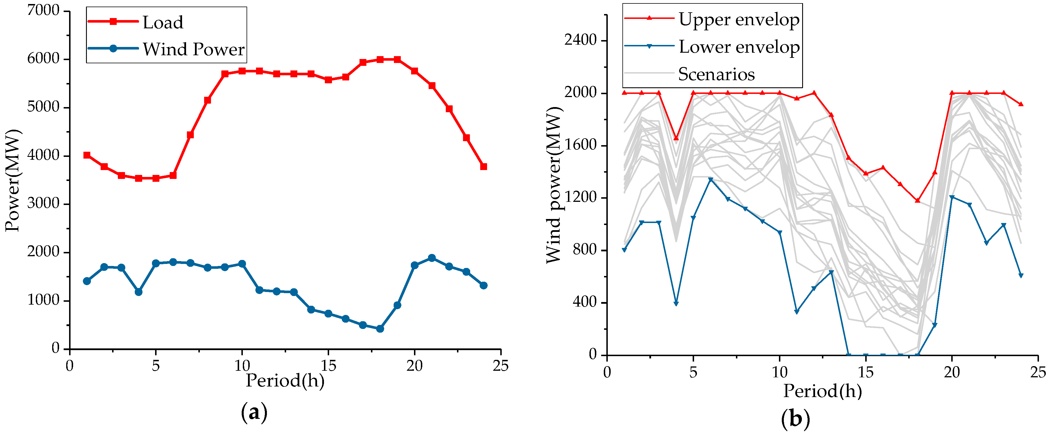
We use wind power to represent VRE. The total installed capacity of wind power is 2000 MW. The predicted wind power and load are shown in Figure 2a. To represent the uncertainty of wind power, 500 stochastic scenarios are generated by the scenario generation method in [26] and then are reduced by the k-means clustering method in [27] to make the SUC formulations computationally tractable. The reduced scenario set has 20 scenarios, which are shown in Figure 2b. The wind power history data are obtained from [28]. The value of lost load is set at 3000 $/MW∙h. The reliability level of the DUC formulations is set at 95%.
According to the analysis in Subsection 3.2, it is clear that the economic criteria are closely related to EACs. For research needs, we assume three sets of EACs, shown in Table 3, to study the impact of EACs on the scheduling results. These three sets have high, medium and low EACs. The EACs in the medium set (EAC-M) are set lower than those in the high set (EAC-H) to represent the decreasing trend of EACs due to the technical progress. The low set (EAC-L) represents the ideal EACs that are low enough to be ignored.
All numerical simulations are coded with the YALMIP toolbox under the MATLAB platform and solved by the solver GUROBI 6.0.5 with a pre-specified optimal tolerance of 0.01% on a Windows-based server with the Xeon ES-1650 (3.50 GHz, six cores) processor.
5.2. Comparisons of the Results Calculated by the Four UC Formulations
Table 4 shows the scheduling results of different UC formulations in terms of six metrics, including total operating costs (TOC), total coal costs (TCC), total EACs (TAC), total startup costs (TSU), expected load not served (ELNS), and expected wind power curtailment (EWC). The total fuel costs consist of the total coal costs and the total EACs. Three sets of EACs are considered for the UC formulations with LLOAF. The prefixes L1, L2, and L3 correspond to EAC-H, EAC-M, and EAC-L.
Under both the stochastic and deterministic UC policies, the formulations with LLOAF have lower total operating costs than the formulations without LLOAF. Under the SUC policy, L1-SUC, L2-SUC, and L3-SUC can reduce the total operating costs by 0.09%, 0.50%, and 2.50% compared to T-SUC. Under the DUC policy, L1-DUC, L2-DUC, and L3-DUC can reduce the total operating costs by 0.10%, 0.47%, and 2.30% compared to T-DUC.
For a better understanding of the composition of the total operating costs, column diagrams of the total operating costs are provided in Figure 3. Figure 3a shows the results of different SUC formulations, Figure 3b shows those of different DUC formulations. The penalty costs of ELNS are so low that are omitted in the diagrams.
As shown in Figure 3a, L1-SUC has the same total startup costs as T-SUC, but has lower total fuel costs (the sum of TAC and TCC) than T-SUC. The advantage of L1-SUC in lower total fuel costs comes from the reduction of EWC because using more wind power can substitute more energy produced by coal-fired units and thus reduces the fuel costs. However, compared to T-SUC, the advantage of L2-SUC and L3-SUC in total operating costs comes from the reduction of the total startup costs. Instead, L2-SUC and L3-SUC have more fuel costs than T-SUC. This is because lower total startup costs mean that during valley load periods fewer units run in the start/stop cycling mode and instead more units run in the low loads, which thus causes the increase of the fuel costs. Besides, the comparisons among L1-SUC, L2-SUC, and L3-SUC show that lower EACs reduce the costs of LLOAF and allow coal-fired units to provide more and cheaper flexible resources for the power system through LLOAF; these cheaper flexible resources can substitute more startups and shutdowns and thus reduce the total operating costs.
As shown in Figure 3b, the results under the DUC policy are similar to those under the SUC policy regarding the comparisons among different formulations with and without LLOAF. But the comparisons between the SUC policy and the DUC policy are provided in the following Subsection 5.4 because they lack comparability here due to without the benchmark provided by the real-time operation simulations.
The comparisons between L2-SUC and L3-SUC show that lower EACs are not necessarily conducive to promoting the use of wind power. The curtailment amount of wind power depends on the equilibrium between marginal benefits and marginal costs of using wind power. On the one hand, wind power can partly substitute the energy produced by the fuel coal and thus reduce the fuel costs. On the other hand, using wind power requires the support of the flexible resources that may be expensive. Lower EACs allow coal-fired units to provide cheaper flexible resources for the power systems but such resources do not necessarily determine the marginal costs of flexible resources. According to the data in the following Subsection 5.3, the marginal costs of flexible resources in the L2-SUC depend on the operating costs of LLOAF; however, the marginal costs of flexible resources in the L3-SUC depend on the expensive startup costs because most increased flexible resources from LLOAF are used to substitute the startups and shutdowns. Due to the more expensive marginal costs of flexible resources, L3-SUC has higher curtailment rate of wind power than L2-SUC. In such a case, one available way to further improve the use of wind power is to improve the marginal benefits of wind power, such as considering the carbon emission costs.
5.3. Analysis of the LLOAF States
The LLOAF states of coal-fired units are analyzed in this subsection to further explain the reasons that cause the differences in the schedules from different formulations. We only compare the schedules from the formulations under the SUC policy in this subsection because the comparisons of the formulations under the DUC policy have the similar results according to Subsection 5.2. Table 5, Table 6 and Table 7 show the LLOAF states of each type of coal-fired units in the L1-SUC, L2-SUC, and L3-SUC, respectively. The index , expressed as Equation (44), is used in these tables to represent the frequency of the LLOAF states for each type of units. The larger indicates that the units of type more frequently adopt the LLOAF mode. If is 0, it indicates that no units of such type adopt the LLOAF mode:
where is the set of the units of type , is the number of scenarios.
To facilitate the analysis of the LLOAF states of coal-fired units, the related parameters are calculated and listed in Table 8, including , , , , and . , and represent for L1-SUC, L2-SUC and L3-SUC. , and represent for L1-SUC, L2-SUC and L3-SUC.
According to the data from Table 5, Table 6, Table 7 and Table 8, the economic criterion for LLOAF, i.e., , has been satisfied by all the units that have adopted the LLOAF mode, including the latter two types of units in the L1-SUC, the latter three types in the L2-SUC and all the types in the L3-SUC. Moreover, when this criterion is only met by a small number of coal-fired units due to high EACs, for instance in the L1-SUC, the increased flexibility from LLOAF cannot reduce the startups and shutdowns and has limited economic value. These data verify that the economic criterion for LLOAF is the precondition for the units to promote the use of wind power by LLOAF and also is the precondition to achieve more economic benefits through LLOAF. Besides, the differences for all types of the units are set at about 0.15, the units with larger capacity have lower and thus have lower ratio . The above data partly illustrate that the units with lower are easier to meet the economic criterion for LLOAF.
The data in Table 5, Table 6 and Table 8 show that the units in the L1-SUC and L2-SUC only adopt the LLOAF mode during valley load periods, and the units with larger more frequently adopt the LLOAF mode during valley load periods, such as the latter three types of units with larger capacity. On the contrary, the former two types of units with smaller capacity have smaller and worse economic performance in the LLOAF, and adopt the start/stop cycling mode during valley load periods instead. Note that the index is used to identify the economics of LLOAF for coal-fired units but only applies to valley load periods. This is because many units run in the low loads during valley load periods, therefore, the economics of the low-load operation impacts the frequency of LLOAF for the units. However, during peak load periods, most units run in their full loads and thus the economics of the low-load operation is not the main factor that determines the operating states of the units. Besides, the values of index for all types of units in the L3-SUC are almost the same due to the ideal EACs, thus, the index fails to identify the economics of LLOAF for the units in the L3-SUC.
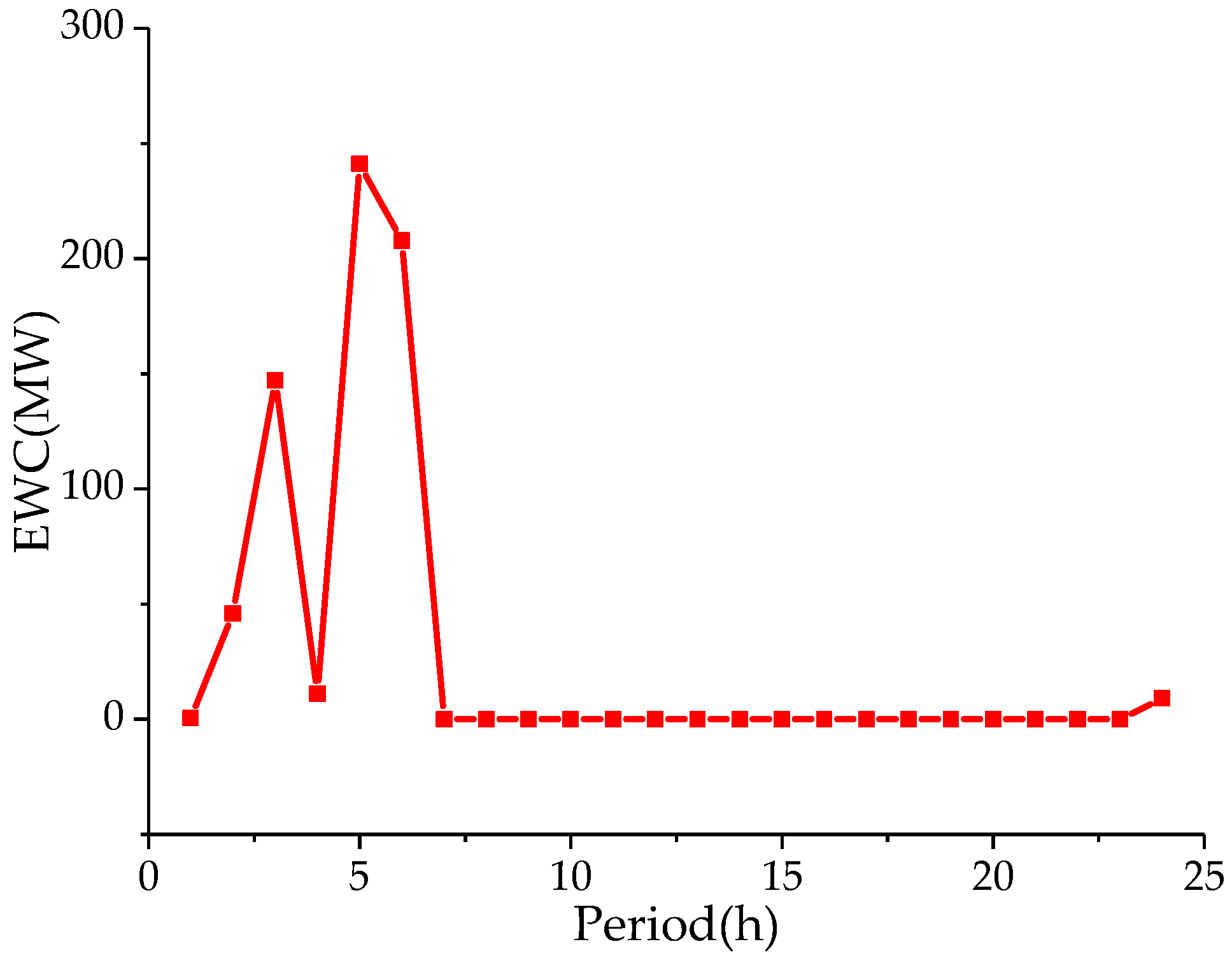
The values of the index can also reflect the adequacy of flexibility from LLOAF. In the L1-SUC and L2-SUC, the values of the index are always small, which indicates that the flexible resources from LLOAF are sufficient even during valley load periods. Therefore, the marginal costs of flexible resources always depend on the operating costs of LLOAF, L1-SUC and L2-SUC can have low curtailment rate of wind power. In the L3-SUC, only the large-capacity units adopt the LLOAF mode during valley load periods as the same as in the L1-SUC and L2-SUC but their values of index are close to 1 in periods 2, 3, 5 and 6. This phenomenon indicates that the increased flexibility from LLOAF is exhausted in these periods and thus the marginal costs of flexible resources depend on expensive startup costs instead of the operating costs of LLOAF. Therefore, L3-SUC has high curtailment rate of wind power in these periods. This deduction is verified by Figure 4.
Though the EACs are ignored in the L3-SUC, the former two types of units with small-capacity still adopt the start/stop cycling mode during valley load periods instead of the LLOAF mode, which is the same as the case in the L1-SUC and L2-SUC. The LLOAF mode has the competitive relationship with the start/stop cycling mode during valley load periods, the scheduling results under different EACs show that the EACs mainly affect the operating mode of medium-capacity units. Fewer EACs are conducive to the LLOAF mode of medium-capacity units, but the LLOAF mode is always less competitive than the start/stop cycling mode for the small-capacity units during valley load periods even under the ideal EACs.
Unlike L1-SUC and L2-SUC, there are some units in the L3-SUC that adopt the LLOAF mode during peak load periods, but such units have small capacity instead of large capacity. This is because it is more economical for the power system to operate the large-capacity units at their full loads and to procure the flexible resources from the small-capacity units during peak load periods. The results show that LLOAF can also apply to the small-capacity units during peak load periods when the EACs are low enough.
5.4. Comparisons of the Real-Time Operation Results for Different Formulations
The schedules directly from the SUC and DUC formulations lack comparability due to their different ways to approximate the uncertainty of wind power. These schedules can be compared when their real-time operation results are simulated by the economic dispatch (ED) simulations. The ED model can be regarded as the SUC model under a single scenario and with the fixed commitment decisions generated by the UC formulation. The expected real-time operation results are calculated by the linear weighted sum of the ED simulation results under each scenario. ED simulations adopt the original 500 scenarios directly generated by the scenario generation method. Table 9 shows the real-time operation performance for the above L-SUC and L-DUC formulations in terms of the same six metrics used in Subsection 5.2.
As shown in Table 9, SUC has lower total operating costs compared to DUC under different EACs or without LLOAF. The advantage of SUC in the total operating costs comes from fewer penalty costs of ELNS relative to DUC.
5.5. Computational Performance
Table 10 shows the computational performance for different UC formulations in terms of four metrics, including the number of integer variables (NIV), the number of continuous variables (NCV), the number of constraints (NCT), and the computing time (CPT).
Compared to T-SUC, L1-SUC, L2-SUC, and L3-SUC have more integer variables and constraints. The computing time of L1-SUC and L2-SUC is 10 and 8 times of that of T-SUC. But the computing time of L3-SUC is less than that of T-SUC. The increased computational burden of L1-SUC and L2-SUC mainly comes from the increased integer variables and constraints. Compared to L1-SUC and L2-SUC, though L3-SUC has the same number of integer variables and constraints, L3-SUC has fewer startups and shutdowns, which can greatly reduce the computational burden from the optimization of the commitment variables and thus increase its computational efficiency.
DUC is far more computationally efficient than SUC. And the additional constraints and variables concerning LLOAF have very limited impact on the computing time of the DUC formulations.
L-SUC can generate more economic schedules but is more time-consuming compared to L-DUC. However, there are some tips that can improve the computational performance of L-SUC. Obviously, the additional variables and constraints concerning LLOAF increase the complexity of L-SUC. L3-SUC is an exception due to the ideal EACs, but L1-SUC and L2-SUC may be more in line with the general situations. According to the analysis in Subsection 5.3, some units do not adopt the LLOAF mode. Therefore, the LLOAF related variables and constraints for such units can be omitted to decrease the complexity of L-SUC. Firstly, we can exclude the units that violate the economic criterion for LLOAF, such as the former three types of units in the L1-SUC. Then, we can exclude the units that rarely adopt the LLOAF mode according to operating experiences, such as the former two types of units in the L2-SUC. With these tips, the complexity of L-SUC can be reduced, the improved L-SUC is referred to as IL-SUC hereinafter. The computational performance for IL-SUC is shown in Table 11, in which the computational performance for L-SUC are also listed for comparisons. As shown in Table 11, IL-SUC reduces the number of integer variables and constraints, and thus reduces the computing time of L-SUC under different EACs.
6. Conclusions
Auxiliary firing is an available measure for coal-fired units to reduce their minimum loads and thus augment their operational flexibility. To implement the evaluation of LLOAF of coal-fired units, we extend the traditional fuel cost model to express the operating costs of LLOAF and present the economic criterion and economic index to assess the economics of LLOAF for a single unit. Then we compare the scheduling results of four UC formulations, i.e., with and without LLOAF under the stochastic and deterministic UC policies, to evaluate the impacts on the scheduling results from the UC policies and from LLOAF. Besides, we investigate the influence of different EACs in the scheduling results to analyze the potential impact of auxiliary firing technology progress on the scheduling results.
We conclude this study with the following remarks:
- (1)
- The economic criterion for LLOAF provides the precondition for coal-fired units to promote the use of VRE through LLOAF. This criterion applies to any situation that involves the power outputs from VRE and provides the precondition for coal-fired units to achieve more benefits through LLOAF.
- (2)
- The economic criterion for LLOAF is highly affected by the ratio between the minimum loads with and without auxiliary firing. This conclusion provides some reference for auxiliary firing retrofit of coal-fired units.
- (3)
- The economic index for LLOAF can be used to assess the economics of LLOAF during valley load periods and provides some intuitional reference for system operators.
- (4)
- Lower EACs reduces the expensive startups and shutdowns of medium-capacity units and thus reduces the total operating costs of the power system though at the price of the increase of the total fuel costs.
- (5)
- Lower EACs do not necessarily ensure low curtailment rate of VRE. When the increased flexibility from LLOAF are mainly used to substitute the startups and shutdowns, the marginal costs of flexible resources may be still determined by the startup costs, resulting in a slightly high curtailment rate of VRE.
- (6)
- LLOAF also applies to small-capacity units under very low EACs. However, unlike large-capacity units, small-capacity units adopt the LLOAF mode in the peak load periods instead of the valley load periods.
- (7)
- The computational efficiency of the L-SUC formulation becomes worse when incorporating the variables and constraints concerning LLOAF, but can be improved with the proposed economic criterion for LLOAF and operating experiences.
We disclose the impact of LLOAF on the scheduling results, which can help the system operators and owners of coal-fired units understand the economic value of LLOAF better. This study uses the general expressions to represent the costs and benefits incurred by LLOAF and thus apply to many auxiliary firing technologies.
The study on the LLOAF in this paper focuses the impact of only fuel costs and neglects other costs caused by LLOAF. From the long-term scale, LLOAF will aggravate the mechanical loss of the units and thus increase their outage probability and maintenance costs. Our future research should quantify the long-term costs and translate them into the short-term operating costs to further improve the economic evaluation of LLOAF.
Acknowledgments
This work was sponsored by the National Natural Science Foundation of China (Grant No. 51677076) and the National Key Research and Development Program of China (Grant No. 2016YFB09001).
Author Contributions
Gang Wang, Dahai You and Suhua Lou proposed the core idea. Gang Wang developed the models, performed the simulations and exported the results. Dahai You, Zhe Zhang and Li Dai provided some important reference material. All authors discussed the results and contributed to writing this paper.
Conflicts of Interest
The authors declare no conflict of interest.
Abbreviations
| CPT | Computing Time |
| CSD | Shut-Down Costs |
| CSU | Start-Up Costs |
| DUC | Deterministic Unit Commitment |
| EAC | Extra Auxiliary Fuel Costs |
| EAC-H | The Set of High Extra Auxiliary Fuel Costs |
| EAC-L | The Set of Low Extra Auxiliary Fuel Costs |
| EAC-M | The Set of Medium Extra Auxiliary Fuel Costs |
| ED | Economic Dispatch |
| ELNS | Expected Load Not Served |
| EWC | Expected Wind Power Curtailment |
| LLOAF | Low-Load Operation with Auxiliary Firing |
| L-DUC | Deterministic Unit Commitment considering LLOAF |
| L-SUC | Stochastic Unit Commitment considering LLOAF |
| L1-DUC | Deterministic Unit Commitment considering LLOAF with EAC-H |
| L1-SUC | Stochastic Unit Commitment considering LLOAF with EAC-H |
| L2-DUC | Deterministic Unit Commitment considering LLOAF with EAC-M |
| L2-SUC | Stochastic Unit Commitment considering LLOAF with EAC-M |
| L3-DUC | Deterministic Unit Commitment considering LLOAF with EAC-L |
| L3-SUC | Stochastic Unit Commitment considering LLOAF with EAC-L |
| MDT | Minimum Down Times |
| MUT | Minimum Up Times |
| NCT | Number of Constraints |
| NCV | Number of Continuous Variables |
| NIV | Number of Integer Variables |
| RD | Ramping Down Limits |
| RU | Ramping Up Limits |
| SUC | Stochastic Unit Commitment |
| TAC | Total Extra Auxiliary Fuel Costs |
| TCC | Total Coal Costs |
| TCE | Tons of Coal Equivalent |
| TOC | Total Operating Costs |
| TSU | Total Start-Up Costs |
| T-DUC | Traditional Deterministic Unit Commitment |
| T-SUC | Traditional Stochastic Unit Commitment |
| UC | Unit Commitment |
| VRE | Variable Renewable Energy |
Nomenclature
| Sets and Indices | |
| Index of units | |
| Index of segments of the piecewise functions | |
| Index of scenarios | |
| Index of time periods | |
| Parameters | |
| Coefficients of the quadratic fuel cost function of unit ($/MW2, $/MW, $) | |
| Price of coal fuel/auxiliary fuel ($/ton) | |
| Startup/shutdown costs of unit ($) | |
| Extra auxiliary fuel costs of unit ($) | |
| Economic index | |
| Frequency of the LLOAF states for the units of type in period | |
| Set of the units of type | |
| Forecast load in period t (MW) | |
| Number of the segments | |
| Number of scenarios | |
| Equilibrium point of unit (MW) | |
| Maximum power output of unit (in segment ) (MW) | |
| Minimum power output of unit with/without LLOAF (MW) | |
| Amount of auxiliary fuel per hour (ton) | |
| Quantile of probability distribution function in period with the proportion | |
| Ramping up/down limit per hour of unit (MW) | |
| Startup/shutdown ramping limit per hour of unit (MW) | |
| Number of periods in one day | |
| Up/ down times of unit (h) | |
| Value of lost load ($/MW∙h) | |
| Renewable power in period and scenario (MW) | |
| Expected renewable power in period (MW) | |
| Arbitrary positive constant | |
| Heat load proportion of auxiliary fuel | |
| Slope and intercept of the linear input-output function ($/MW, $) | |
| Load rate of minimum load with/without auxiliary firing | |
| Probability of scenario | |
| Variables | |
| Startup/shutdown cost function of unit ($) | |
| Fuel costs including/excluding extra auxiliary fuel costs of unit ($) | |
| Binary variable; LLOAF state of unit in period (and scenario ) | |
| Amount of lost load in period (and scenario ) (MW) | |
| Power output of unit in period (and scenario ) (MW) | |
| Amount of coal fuel per hour (ton) | |
| Total fuel consumption per hour of power output P of unit (ton) | |
| Up reserve provided by unit in period (MW) | |
| Binary variable; commitment decision of unit in period (and scenario ) | |
| Renewable power curtailment variable in period and scenario (MW) | |
References
- IRNEA. Roadmap for a Renewable Energy Future. Available online: http://www.irena.org/DocumentDownloads/Publications/IRENA_REmap_2016_edition_report.pdf (accessed on 30 August 2017).
- IRNEA. Renewable Energy Prospects: Germany. Available online: http://www.irena.org/DocumentDownloads/Publications/IRENA_REmap_Germany_report_2015.pdf (accessed on 30 August 2017).
- IRNEA. Renewable Energy Prospects: USA. Available online: http://www.irena.org/REmap/IRENA_REmap_USA_report_2015.pdf (accessed on 30 August 2017).
- NERL. Integrating Variable Renewable Energy: Challenges and Solutions. Available online: http://www.nrel.gov/docs/fy13osti/60451.pdf (accessed on 30 August 2017).
- Xu, L.; Tretheway, D. Flexible Ramping Products: California ISO. Available online: https://www.caiso.com/Documents/DraftFinalProposal-FlexibleRampingProduct.pdf (accessed on 30 August 2017).
- Navid, N.; Rosenwald, G. Ramp Capability Product Design for MISO Markets. Available online: https://www.misoenergy.org/Library/Repository/Communication%20Material/Key%20Presentations%20and%20Whitepapers/Ramp%20Product%20Conceptual%20Design%20Whitepaper.pdf (accessed on 30 August 2017).
- Northeast China Energy Regulatory Bureau of National Energy Administration. Pilot Reform Scheme of the Northeast Electric Power Auxiliary Service Market. Available online: http://dbj.nea.gov.cn/nyjg/hyjg/201611/t20161124_2580781.html (accessed on 30 August 2017).
- Agora Energiewende. Flexibility in Thermal Power Plants-with a Focus on Existing Coal-Fired Power Plants. Available online: https://www.agora-energiewende.de/fileadmin/Projekte/2017/Flexibility_in_thermal (accessed on 30 August 2017).
- National Energy Administrator. Notice on Pilot Project of Thermal Power Flexibility Transformation. Available online: http://zfxxgk.nea.gov.cn/auto84/201607/t20160704_2272.htm (accessed on 30 August 2017).
- National Development and Reform Commission. 13th Five-Year Plan of Renewable Energy Development. Available online: http://www.sdpc.gov.cn/zcfb/zcfbtz/201612/W020161216659579206185.pdf (accessed on 30 August 2017).
- Bergins, C.; Agraniotis, M.; Kakaras, E.; Leisse, A. Improving Flexibility of Lignite Boilers through Firing System Optimisation and Retrofit. Available online: http://pennwell.sds06.websds.net/2015/amsterdam/papers/T6S1O2-paper.pdf (accessed on 30 August 2017).
- Lin, B.; Gao, S.; Wu, H. Research and application of the sequential control logic of micro oil ignition system for opposed firing supercritical boiler. In Proceedings of the 2016 International Symposium on Advances in Electrical, Electronics and Computer Engineering, Guangzhou, China, 12–13 March 2016; pp. 38–41. [Google Scholar]
- Yan, K.; Wu, X.; Hoadley, A.; Hoadley, A.; Xu, X.; Zhang, J.; Zhang, L. Sensitivity analysis of oxy-fuel power plant system. Energy Convers. Manag. 2015, 98, 138–150. [Google Scholar] [CrossRef]
- Bergins, C.; Leisse, A.; Rehfeldt, S. How to Utilize Low Grade Coals below 1000 kcal/kg? Available online: http://pennwell.sds06.websds.net/2014/cologne/pge/papers/T4S4O50-paper.pdf (accessed on 30 August 2017).
- Marneris, I.; Biskas, P.; Bakirtzis, A. Stochastic and Deterministic Unit Commitment Considering Uncertainty and Variability Reserves for High Renewable Integration. Energies 2017, 10, 140. [Google Scholar] [CrossRef]
- Liao, S.; Li, Z.; Li, G.; Wang, J.; Wu, X. Modeling and optimization of the medium-term units commitment of thermal power. Energies 2015, 8, 12848–12864. [Google Scholar] [CrossRef]
- Dvorkin, Y.; Pandžić, H.; Ortega-Vazquez, M.A.; Kirschen, D. A hybrid stochastic/interval approach to transmission-constrained unit commitment. IEEE Trans. Power Syst. 2015, 30, 621–631. [Google Scholar] [CrossRef]
- Wood, A.J.; Wollenberg, B.F.; Sheblé, G.B. Power Generation Operation and Control, 2nd ed.; Wiley: Hoboken, NJ, USA, 2003; pp. 9–13. [Google Scholar]
- Attaviriyanupap, P.; Kita, H.; Tanaka, E.; Hasegawa, J. A hybrid EP and SQP for dynamic economic dispatch with nonsmooth fuel cost function. IEEE Trans. Power Syst. 2002, 17, 411–416. [Google Scholar] [CrossRef]
- Morales-España, G.; Ramírez-Elizondo, L.; Hobbs, B.F. Hidden power system inflexibilities imposed by traditional unit commitment formulations. Appl. Energy 2017, 191, 223–238. [Google Scholar] [CrossRef]
- Klein, J.B. The Use of Heat Rates in Production Cost Modeling and Market Modeling. Available online: http://www.energy.ca.gov/papers/98-04-07_HEATRATE.PDF (accessed on 30 August 2017).
- Constantinescu, E.M.; Zavala, V.M.; Rocklin, M.; Lee, S.; Anitescu, M. A Computational Framework for Uncertainty Quantification and Stochastic Optimization in Unit Commitment with Wind Power Generation. IEEE Trans. Power Syst. 2011, 26, 431–441. [Google Scholar] [CrossRef]
- Ruiz, P.A.; Philbrick, C.R.; Zak, E.; Cheung, K.W.; Sauer, P.W. Uncertainty management in the unit commitment problem. IEEE Trans. Power Syst. 2009, 24, 642–651. [Google Scholar] [CrossRef]
- Wu, L. A Tighter Piecewise Linear Approximation of Quadratic Cost Curves for Unit Commitment Problems. IEEE Trans. Power Syst. 2011, 26, 2581–2583. [Google Scholar] [CrossRef]
- Doherty, R.; O’malley, M. A new approach to quantify reserve demand in systems with significant installed wind capacity. IEEE Trans. Power Syst. 2005, 20, 587–595. [Google Scholar] [CrossRef]
- Pierre, P.; Henrik, M.; Aa, N.H.; George, P.; Bernd, K. From probabilistic forecasts to statistical scenarios of short-term wind power production. Wind Energy 2010, 12, 51–62. [Google Scholar]
- Baringo, L.; Conejo, A.J. Correlated wind-power production and electric load scenarios for investment decisions. Appl. Energy 2013, 101, 475–482. [Google Scholar] [CrossRef]
- Eastern Wind Integration and Transmission Study—NREL Data. Available online: https://www.nrel.gov/grid/eastern-wind-data.html (accessed on 30 August 2017).
Figure 1.
Fuel cost curve for LLOAF.
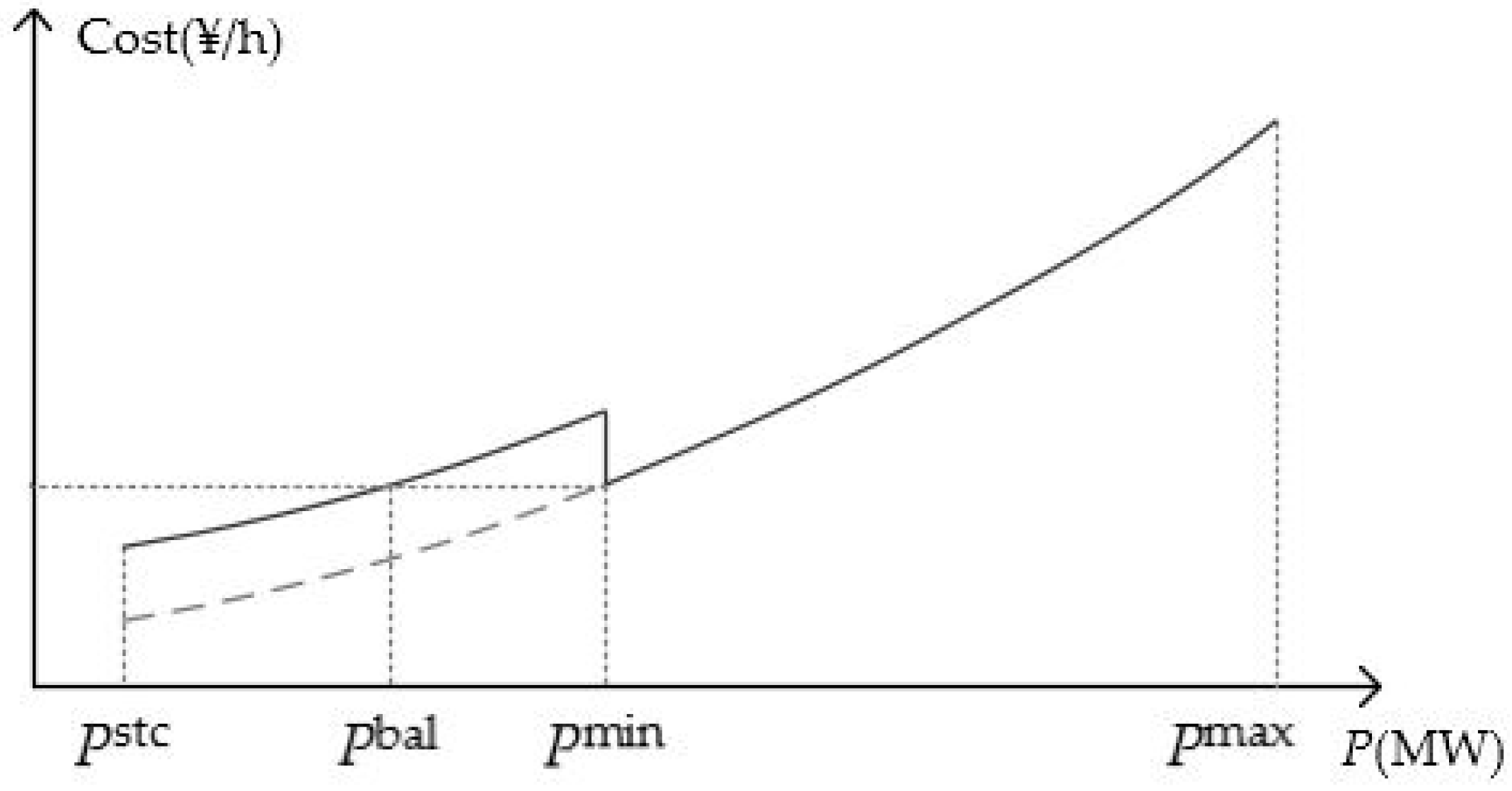
Figure 2.
Load and wind power: (a) Predicted load and wind power; (b) Representation of wind uncertainty over time.
Figure 2.
Load and wind power: (a) Predicted load and wind power; (b) Representation of wind uncertainty over time.

Figure 3.
Column diagrams of the total operating costs: (a) results of different SUC formulations; (b) results of different DUC formulations.
Figure 3.
Column diagrams of the total operating costs: (a) results of different SUC formulations; (b) results of different DUC formulations.
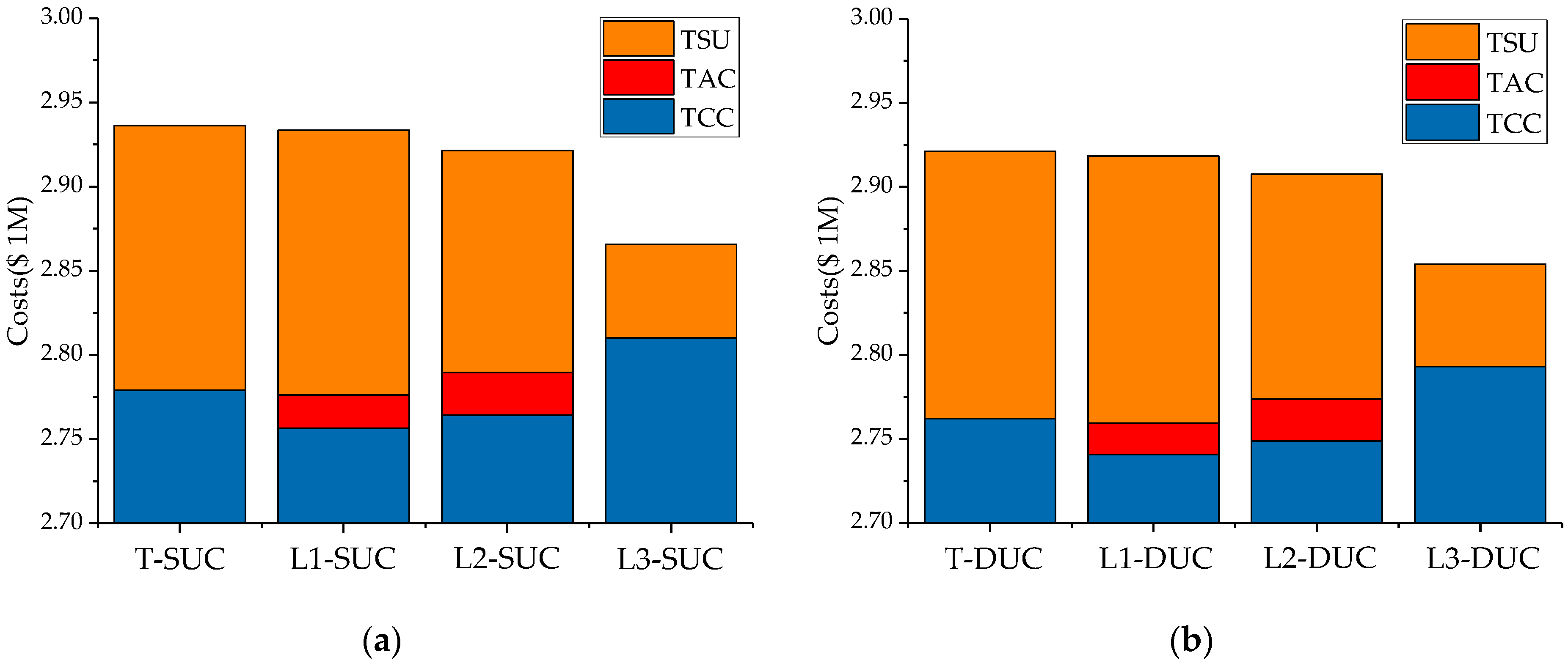
Figure 4.
Expected wind power curtailment in each period in the L3-SUC.

Table 1.
Technical parameters of the units.
| Type | Index | (MW) | (MW) | (MW) | MUT (h) | MDT (h) | RU (MW/h) | RD (MW/h) |
|---|---|---|---|---|---|---|---|---|
| 1 | 1–2 | 135 | 90 | 70 | 5 | 5 | 70 | 70 |
| 2 | 3–7 | 200 | 120 | 90 | 8 | 8 | 100 | 100 |
| 3 | 8–12 | 300 | 180 | 135 | 10 | 10 | 150 | 150 |
| 4 | 13–16 | 350 | 200 | 148 | 24 | 24 | 175 | 175 |
| 5 | 17–20 | 600 | 280 | 190 | 24 | 24 | 300 | 300 |
Table 2.
Economic parameters of the units.
| Type | a ($/MW2) | b ($/MW) | c ($) | CSU ($) | CSD ($) |
|---|---|---|---|---|---|
| 1 | 0.00931 | 28.83 | 469.23 | 11,154 | 0 |
| 2 | 0.00666 | 28.35 | 623.23 | 16,615 | 0 |
| 3 | 0.00337 | 28.18 | 807.23 | 25,385 | 0 |
| 4 | 0.00454 | 27.28 | 872.77 | 29,538 | 0 |
| 5 | 0.00202 | 26.80 | 1311.38 | 51,077 | 0 |
Table 3.
Three sets of EACs.
| Type | 1 | 2 | 3 | 4 | 5 |
|---|---|---|---|---|---|
| EAC-H ($) | 690 | 950 | 1380 | 1470 | 2145 |
| EAC-M ($) | 460 | 633 | 920 | 980 | 1430 |
| EAC-L ($) | 0 | 0 | 0 | 0 | 0 |
Table 4.
The results of different formulations.
| TOC ($ 1M) | TCC ($ 1M) | TAC ($ 1M) | TSU ($ 1M) | ELNS (MW∙h) | EWC (MW∙h) | |
|---|---|---|---|---|---|---|
| T-SUC | 2.9361 | 2.7770 | 0 | 0.1571 | 0.6703 | 883 |
| L1-SUC | 2.9335 | 2.7546 | 0.0197 | 0.1571 | 0.6703 | 82 |
| L2-SUC | 2.9214 | 2.7623 | 0.0254 | 0.1317 | 0.6703 | 67 |
| L3-SUC | 2.8657 | 2.8081 | 0 | 0.0555 | 0.6703 | 663 |
| T-DUC | 2.9213 | 2.7620 | 0 | 0.1592 | 0 | 860 |
| L1-DUC | 2.9184 | 2.7406 | 0.0186 | 0.1592 | 0 | 88 |
| L2-DUC | 2.9075 | 2.7488 | 0.0249 | 0.1339 | 0 | 60 |
| L3-DUC | 2.8540 | 2.7930 | 0 | 0.0610 | 0 | 617 |
Table 5.
The LLOAF states of different types of coal-fired units in the L1-SUC.
| Type | 1 h | 2 h | 3 h | 4 h | 5 h | 6 h | 7–23 h | 24 h |
|---|---|---|---|---|---|---|---|---|
| 1 | 0 | 0 | 0 | 0 | 0 | 0 | 0 | 0 |
| 2 | 0 | 0 | 0 | 0 | 0 | 0 | 0 | 0 |
| 3 | 0 | 0 | 0 | 0 | 0 | 0 | 0 | 0 |
| 4 | 0 | 0.0375 | 0.125 | 0 | 0.2375 | 0.2 | 0 | 0.013 |
| 5 | 0.0125 | 0.175 | 0.4 | 0.0625 | 0.5625 | 0.5125 | 0 | 0.025 |
Table 6.
The LLOAF states of different types of coal-fired units in the L2-SUC.
| Type | 1 h | 2 h | 3 h | 4 h | 5 h | 6 h | 7–23 h | 24 h |
|---|---|---|---|---|---|---|---|---|
| 1 | 0 | 0 | 0 | 0 | 0 | 0 | 0 | 0 |
| 2 | 0 | 0 | 0 | 0 | 0 | 0 | 0 | 0 |
| 3 | 0.025 | 0.075 | 0.25 | 0.025 | 0.325 | 0.325 | 0 | 0 |
| 4 | 0 | 0.0875 | 0.3 | 0.0125 | 0.475 | 0.4375 | 0 | 0.0125 |
| 5 | 0.0375 | 0.4875 | 0.6875 | 0.1625 | 0.8 | 0.75 | 0 | 0.0875 |
Table 7.
The LLOAF states of different types of coal-fired units in the L3-SUC.
| Type | 1 h | 2 h | 3 h | 4 h | 5 h | 6 h | 7 h | 8 h | 9–20 h | 21 h | 22 h | 23 h | 24 h |
|---|---|---|---|---|---|---|---|---|---|---|---|---|---|
| 1 | 0 | 0 | 0 | 0 | 0 | 0 | 0 | 0 | X 1 | 0 | 0 | 0 | 0 |
| 2 | 0 | 0 | 0 | 0 | 0 | 0 | 0 | 0 | X 1 | 0 | 0 | 0 | 0 |
| 3 | 1 | 1 | 1 | 1 | 1 | 1 | 1 | 1 | X 1 | 0.93 | 0.99 | 1 | 1 |
| 4 | 1 | 1 | 1 | 1 | 1 | 1 | 1 | 0.66 | 0 | 0.49 | 0.9 | 1 | 1 |
| 5 | 0.14 | 0.85 | 0.95 | 0.46 | 0.95 | 1 | 0.06 | 0 | 0 | 0 | 0 | 0.05 | 0.33 |
1 X means that not all the values are zero during these periods.
Table 8.
The parameters of coal-fired units concerning LLOAF.
| Type | (MW) | (MW) | (MW) | (MW) | (MW) | (MW) | |||
|---|---|---|---|---|---|---|---|---|---|
| 1 | 135 | 90 | 70 | 67 | 75 | 90 | −0.022 | 0.007 | 0.148 |
| 2 | 200 | 120 | 90 | 88 | 99 | 120 | −0.010 | 0.015 | 0.150 |
| 3 | 300 | 180 | 135 | 133 | 149 | 180 | −0.007 | 0.020 | 0.150 |
| 4 | 350 | 200 | 148 | 149 | 166 | 200 | 0.003 | 0.029 | 0.149 |
| 5 | 600 | 280 | 190 | 203 | 229 | 280 | 0.022 | 0.043 | 0.150 |
Table 9.
The real-time operation performance for different UC formulations.
| TOC ($ 1M) | TCC ($ 1M) | EAC ($ 1M) | TSU ($ 1M) | ELNS (MW∙h) | EWC (MW∙h) | |
|---|---|---|---|---|---|---|
| T-SUC-ED | 3.0933 | 2.7869 | 0 | 0.1571 | 50 | 974 |
| T-DUC-ED | 3.2636 | 2.7828 | 0 | 0.1592 | 107 | 974 |
| L1-SUC-ED | 2.9333 | 2.7621 | 0.0219 | 0.1571 | 50 | 83 |
| L1-DUC-ED | 3.1014 | 2.7580 | 0.0219 | 0.1592 | 107 | 83 |
| L2-SUC-ED | 2.9288 | 2.7694 | 0.0269 | 0.1317 | 44 | 58 |
| L2-DUC-ED | 3.0737 | 2.7664 | 0.0269 | 0.1339 | 93 | 58 |
| L3-SUC-ED | 2.8715 | 2.8186 | 0 | 0.0555 | 18 | 747 |
| L3-DUC-ED | 2.8151 | 2.8160 | 0 | 0.0610 | 33 | 747 |
Table 10.
Computational performance for different UC formulations.
| NIV | NCV | NCT | CPT (s) | |
|---|---|---|---|---|
| T-SUC | 480 | 38,900 | 253,504 | 186 |
| L1-SUC | 10,080 | 38,900 | 282,304 | 1895 |
| L2-SUC | 10,080 | 38,900 | 282,304 | 1504 |
| L3-SUC | 10,080 | 38,900 | 282,304 | 139 |
| T-DUC | 480 | 2880 | 15,520 | 42 |
| L1-DUC | 960 | 2880 | 16,960 | 46 |
| L2-DUC | 960 | 2880 | 16,960 | 58 |
| L3-DUC | 960 | 2880 | 16,960 | 7 |
Table 11.
Computational performance for improved L-SUC formulations.
| NIV | NCV | NCT | CPT (s) | |
|---|---|---|---|---|
| L1-SUC | 10,080 | 38,900 | 282,304 | 1895 |
| IL1-SUC | 4320 | 38,900 | 265,024 | 1102 |
| L2-SUC | 10,080 | 38,900 | 282,304 | 1504 |
| IL2-SUC | 6720 | 38,900 | 272,224 | 1216 |
© 2017 by the authors. Licensee MDPI, Basel, Switzerland. This article is an open access article distributed under the terms and conditions of the Creative Commons Attribution (CC BY) license (http://creativecommons.org/licenses/by/4.0/).
Share and Cite
MDPI and ACS Style
Wang, G.; You, D.; Lou, S.; Zhang, Z.; Dai, L. Economic Valuation of Low-Load Operation with Auxiliary Firing of Coal-Fired Units. Energies 2017, 10, 1317. https://doi.org/10.3390/en10091317
AMA Style
Wang G, You D, Lou S, Zhang Z, Dai L. Economic Valuation of Low-Load Operation with Auxiliary Firing of Coal-Fired Units. Energies. 2017; 10(9):1317. https://doi.org/10.3390/en10091317
Chicago/Turabian StyleWang, Gang, Daihai You, Suhua Lou, Zhe Zhang, and Li Dai. 2017. "Economic Valuation of Low-Load Operation with Auxiliary Firing of Coal-Fired Units" Energies 10, no. 9: 1317. https://doi.org/10.3390/en10091317
Note that from the first issue of 2016, this journal uses article numbers instead of page numbers. See further details here.