Study and Analysis of an Intelligent Microgrid Energy Management Solution with Distributed Energy Sources

 ,
,  , ,
, , 
Abstract
:1. Introduction
2. Load Management
2.1. Classification of Loads
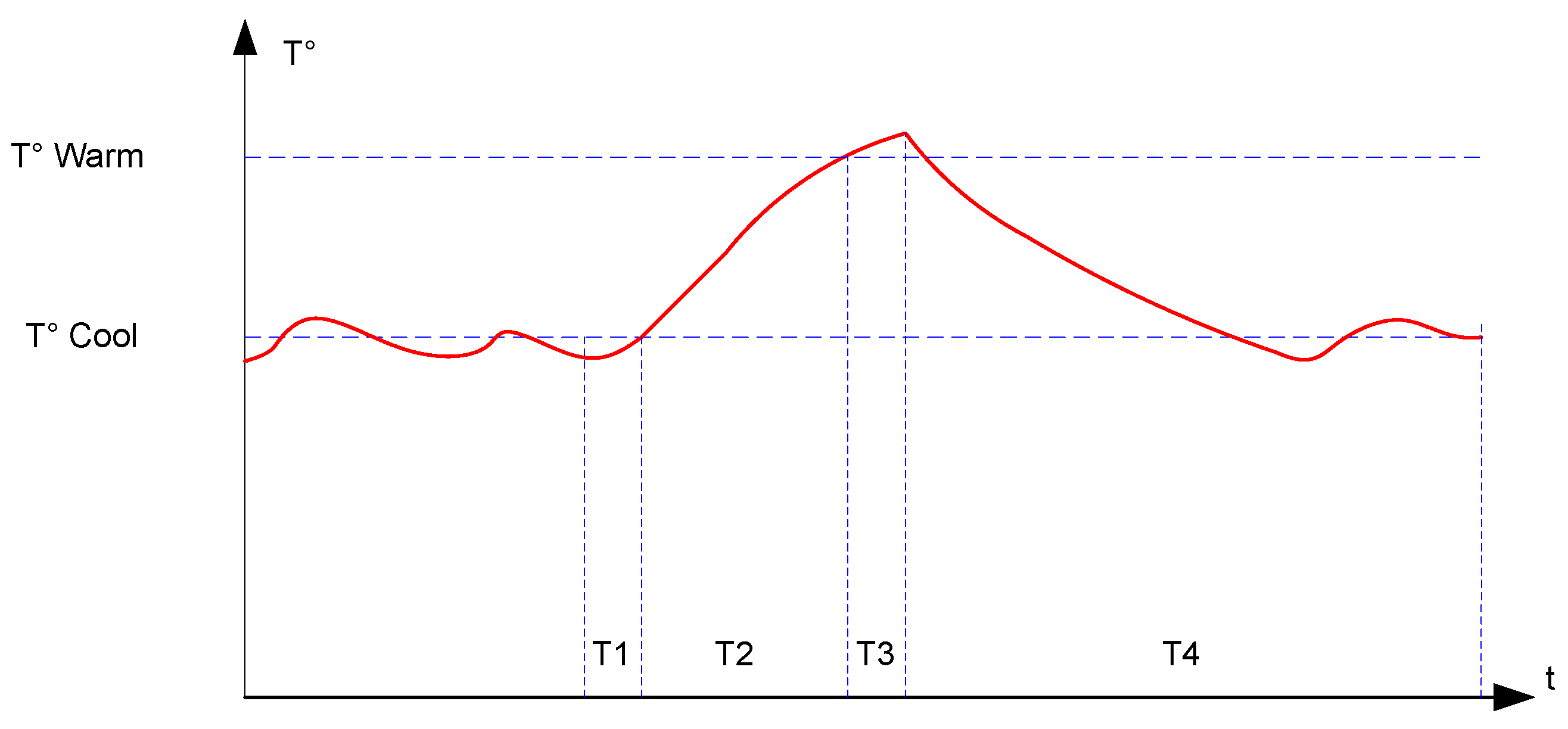
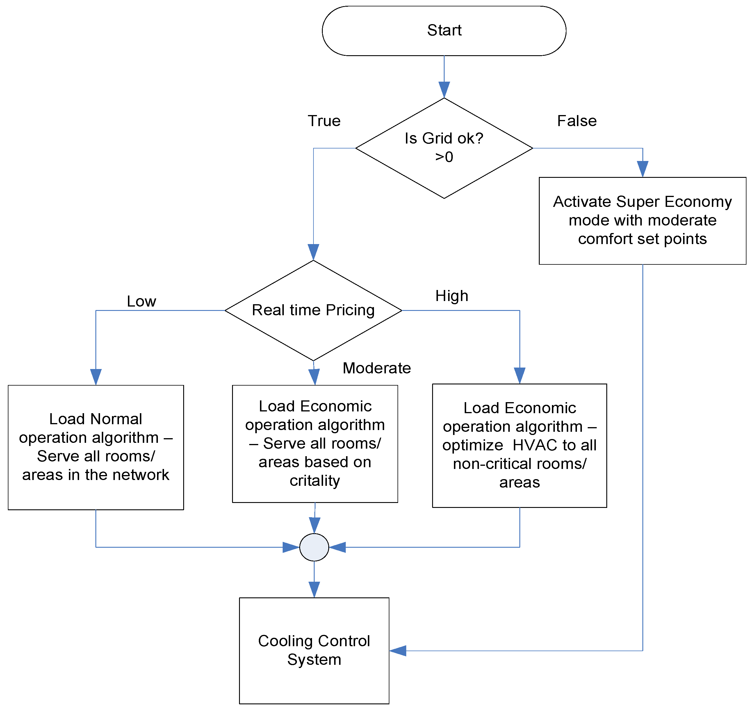
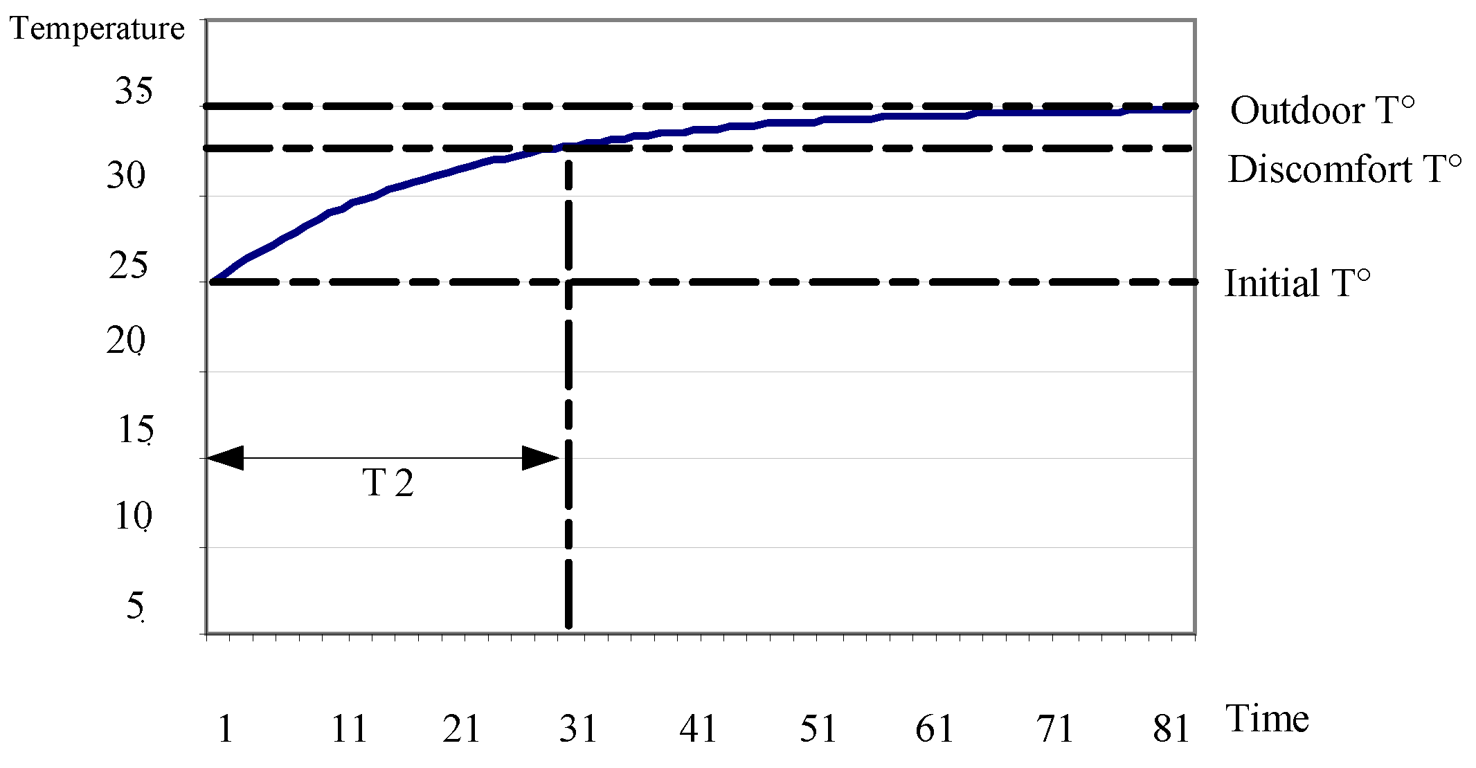
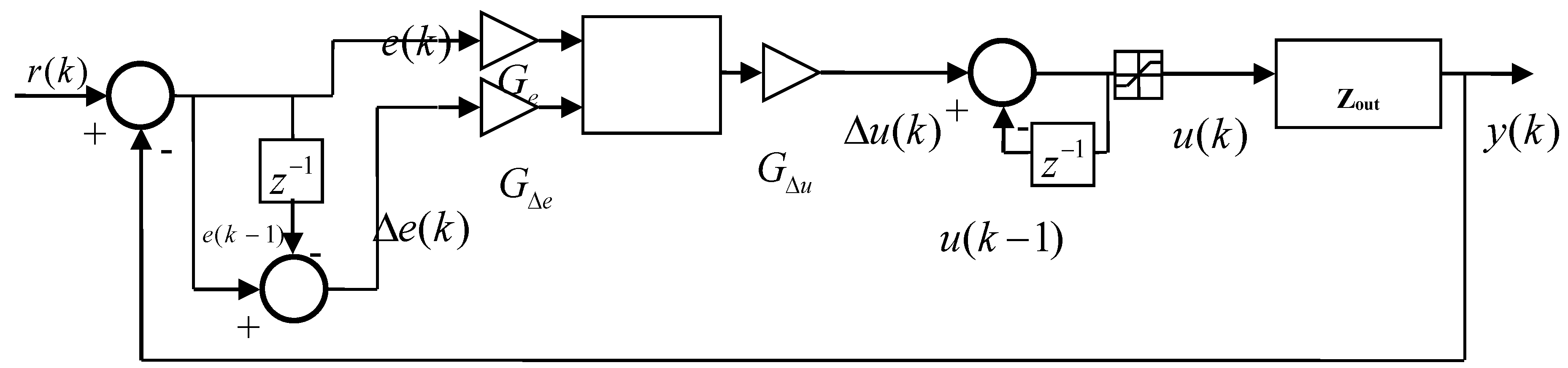
2.2. Control of Air Conditioning Loads
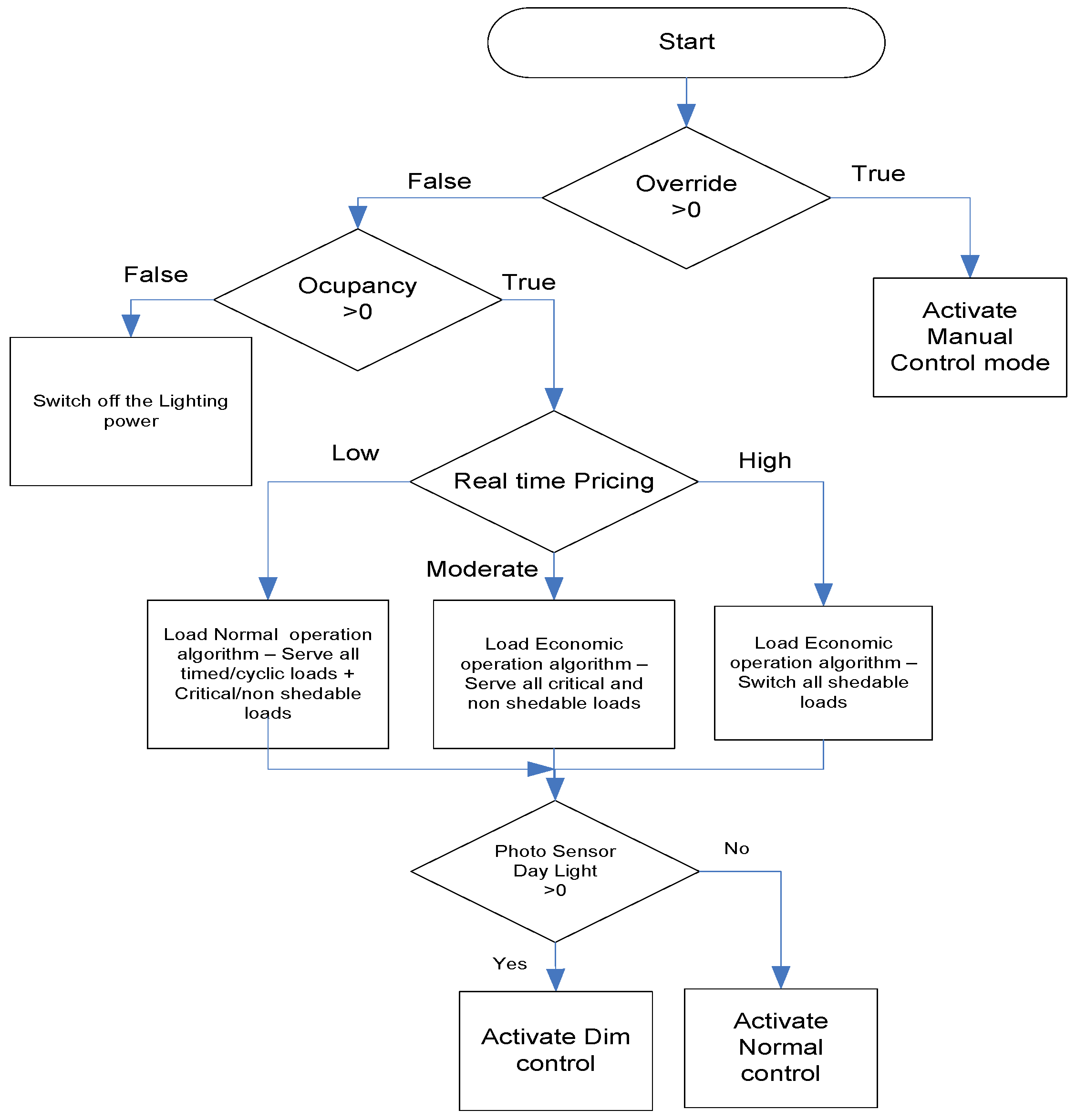
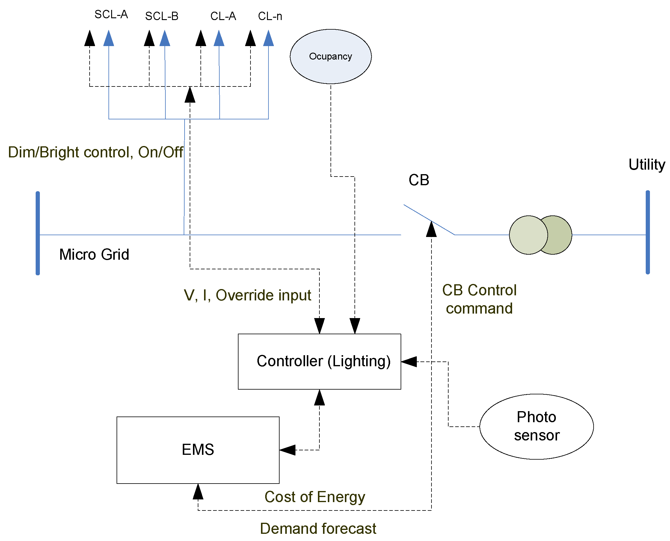
2.3. Control of Lighting Loads
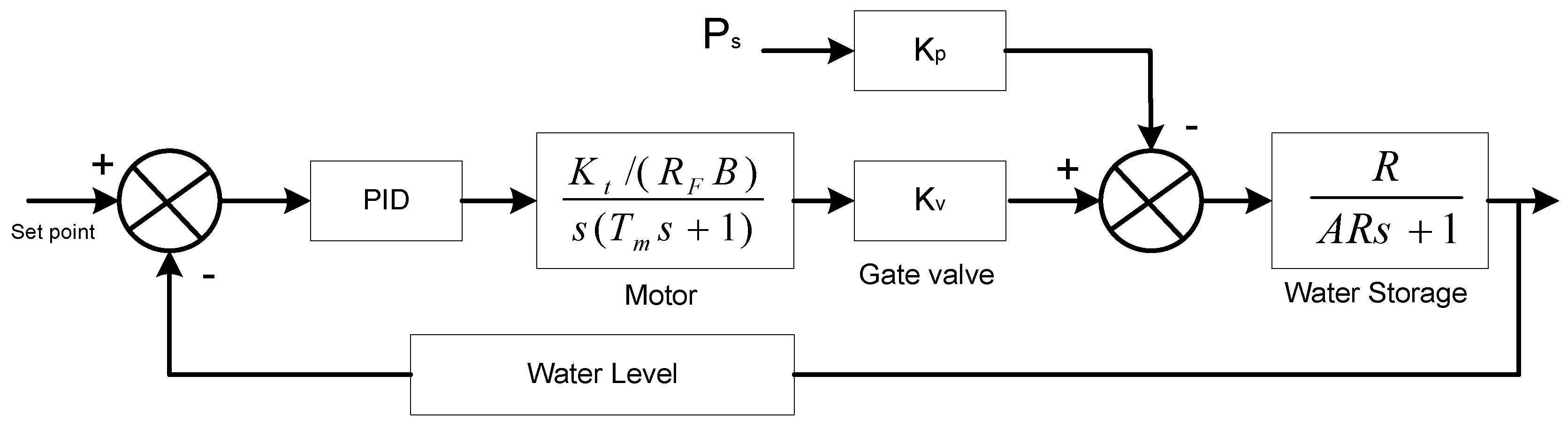
2.4. Control of Water Pump Loads
3. Modes of Operation
3.1. On Grid Mode of Operation
3.2. Off Grid Mode of Operation
Stability and Power Sharing
4. Simulation Results
5. Experimental Results
6. Conclusions
Acknowledgments
Author Contributions
Conflicts of Interest
List of Acronyms
| EMS | Energy Management System |
| PV | Photovoltaic |
| UPS | Uninterrupted Power Supply |
| DES | Distributed Energy Sources |
| BESS | Battery Energy Storage System |
| DER | Distributed Energy Resources |
| DRM | Demand and Response Management |
| SOC | State of Charge |
| DG | Diesel Generator |
| PCC | Point of Common Coupling |
| ESS | Energy Storage System |
| HMI | Human Machine Interface |
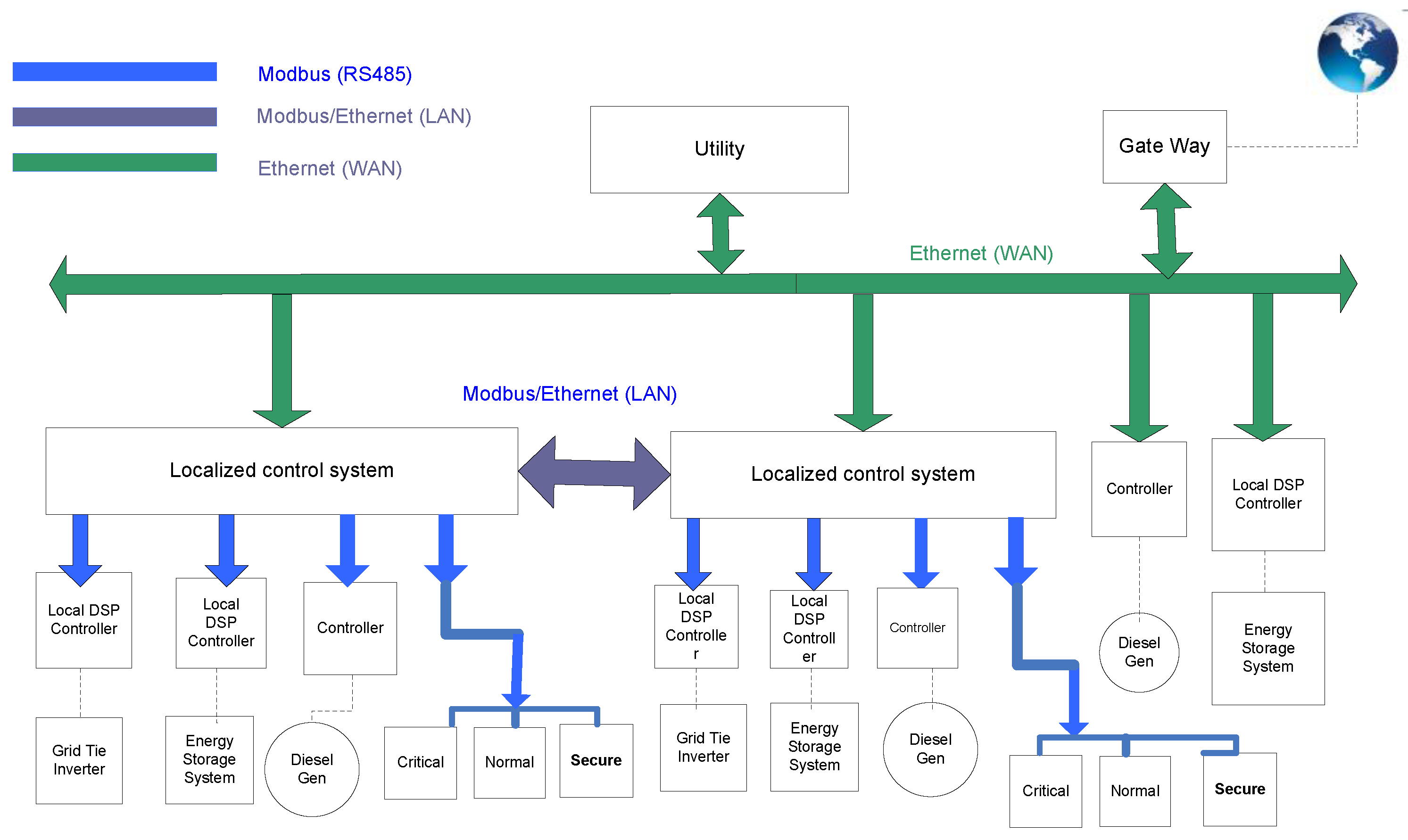
| TCP | Transmission Control Protocol |
| IP | Internet Protocol |
| PLC | Programmable Logic Controller |
References
- Gaurav, S.; Chirag, B.; Aman, L.; Umashankar, S.; Swaminathan, G. Energy Management of PV–Battery Based Microgrid System. Procedia Technol. 2015, 21, 103–111. [Google Scholar] [CrossRef]
- Swaminathan, G.; Ramesh, V.; Umashankar, S. Performance Improvement of Micro Grid Energy Management System using Interleaved Boost Converter and P&O MPPT Technique. Int. J. Renew. Energy Res. 2016, 6, 2. [Google Scholar]
- Mihet-Popa, L.; Isleifsson, F.; Groza, V. Experimental Testing for Stability Analysis of Distributed Energy Resorces Components with Storage Devices and Loads. In Proceedings of the IEEE I2MTC-International Instrumentation & Measurement Technology Conference, Gratz, Austria, 12–15 May 2012; pp. 588–593. [Google Scholar]
- Mihet-Popa, L.; Bindner, H. Simulation models developed for voltage control in a distribution network using energy storage systems for PV penetration. In Proceedings of the 39th Annual Conference of the IEEE Industrial Electronics Society-IECON’13, Vienna, Austria, 10–13 November 2013; pp. 7487–7492. [Google Scholar]
- Zong, Y.; Mihet-Popa, L.; Kullman, D.; Thavlov, A.; Gehrke, O.; Bindner, H. Model Predictive Controller for Active Demand Side Management with PV Self-Consumption in an Intelligent Building. In Proceedings of the IEEE PES Innovative Smart Grid Technologies Europe, Berlin, Germany, 14–17 October 2012. [Google Scholar]
- Wu, B.; Kouro, S.; Malinowski, M.; Pou, J.; Franquelo, L.G.; Gopakumar, K.; Rodriguez, J. Recent advanncement in industrial application of multilevel converter. IEEE Trans. Ind. Electron. 2010, 57, 2553–2580. [Google Scholar]
- Kim, S.-K.; Jeon, J.-H.; Cho, C.-H.; Kon, S.-H. Dynamic modeling and controls of a grid-connected hybrid genration system for versatile power transfers. IEEE Trans. Ind. Electron. 2008, 55, 1677–1688. [Google Scholar] [CrossRef]
- Sanjeevikumar, P.; Grandi, G.; Blaabjerg, F.; Wheeler, P.; Hammami, M.; Siano, P. A Comprehensive Analysis and Hardware Implementation of Control Strategies for High Output Voltage DC-DC Boost Power Converter. Int. J. Comput. Intell. Syst. (IJCIS) 2017, 10, 140–152. [Google Scholar]
- Hemanshu, R.; Hossain, M.J.; Mahmud, M.A.; Gadh, R. Control for Microgrids with Inverter Connected Renewable energy Resources. In Proceedings of the IEEE PES General Meeting, Washington, DC, USA, 27–31 July 2014. [Google Scholar]
- Adhikari, S.; Li, F.X. Coordinated V-f and P-Q Control of Solar Photovoltaic Generators With MPPT and Battery Storage in Microgrids. IEEE Trans. Smart Grid 2014, 5, 1270–1281. [Google Scholar] [CrossRef]
- Yang, M.; Li, H.P. Analysis of Parallel Photovoltaic Inverters with Improved Droop Control Method. In Proceedings of the International Conference on Modeling and Applied Mathematics (MSAM 2015), Phuket, Thailand, 23–24 August 2015; Atlantis Press: Amsterdam, The Netherlands. [Google Scholar]
- Ganesan, S.; Ramesh, V.; Umashankar, S.; Sanjeevikumar, P. Fuzzy Based Micro Grid Energy Management System using Interleaved Boost Converter and Three Level NPC Inverter with Improved Grid Voltage Quality. LNEE Springer J. 2016. Accepted for Publication. [Google Scholar]
- Hosseinzadeh, M.; Salmasi, F.R. Power management of an isolated hybrid AC/DC micro-grid with fuzzy control of battery banks. IET Renew. Power Gener. 2015, 9, 484–493. [Google Scholar] [CrossRef]
- Guo, Z.Q.; Sha, D.S.; Liao, X.Z. Energy management by using point of common coupling frequency as an agent for islanded microgrids. IET Power Electron. 2014, 7, 2111–2122. [Google Scholar] [CrossRef]
- Chen, C.; Duan, S.; Cai, T.; Liu, B.; Hu, G. Smart energy management system for optimal microgrid economic operation. IET Renew. Power Gener. 2011, 5, 258–267. [Google Scholar] [CrossRef]
- Karavas, C.S.; Kyriakarakos, G.; Arvanitis, K.G.; Papadakis, G. A multi-agent decentralized energy management system based on distributed intelligence for the design and control of autonomous polygeneration microgrids. Energy Convers. Manag. 2015, 103, 166–179. [Google Scholar] [CrossRef]
- Singh, S.; Singh, M.; Kaushik, S.C. Optimal power scheduling of renewable energy systems in microgrids using distributed energy storage system. IET Renew. Power Gener. 2016, 10, 1328–1339. [Google Scholar] [CrossRef]
- Yang, H.-T.; Liao, J.-T. Hierarchical energy management mechanisms for an electricity market with microgrids. J. Eng. 2014. [Google Scholar] [CrossRef]
- Kanchev, H.; Lu, D.; Colas, F.; Lazarov, V.; Francois, B. Energy Management and Operational Planning of a Microgrid With a PV-Based Active Generator for Smart Grid Application. IEEE Trans. Ind. Electron. 2011, 58. [Google Scholar] [CrossRef] [Green Version]
- Ishigaki, Y.; Kimura, Y.; Matsusue, I.; Miyoshi, H.; Yamagishi, K. Optimal Energy Management System for Isolated Micro Grids. SEI Tech. Rev. 2014, 78, 73–78. [Google Scholar]
- Asghari, B.; Guo, F.; Hooshmand, A.; Patil, R.; Pourmousavi, S.A.; Shi, D.; Ye, Y.Z.; Sharma, R. Resilient Microgrid Management Solution. NEC Tech. J. 2016, 10, 103–106. [Google Scholar]
- Zhang, Y.; Gatsis, N.; Giannakis, G.B. Robust Energy Management for Microgrids With High-Penetration Renewables. IEEE Trans. Sustain. Energy 2013, 4, 944–953. [Google Scholar] [CrossRef]
- Shi, W.B.; Lee, E.-K.; Yao, D.Y.; Huang, R.; Chu, C.-C.; Gadh, R. Evaluating Microgrid Management and Control with an Implementable Energy Management System. In Proceedings of the International Conference on Smart Grid Communications, Venice, Italy, 3–6 November 2014. [Google Scholar]
- Tantimaporn, T.; Jiyajan, S.; Payakkarueng, S. Microgrid Islanding Operation Experience. In Proceedings of the 22nd International Conference on Electricity Distribution (CRIED 2013), Stockholm, Sweden, 10–13 June 2013. [Google Scholar]
- Lidula, N.W.A.; Rajapakse, A.D. Microgrids research: A review of experimental microgrids and test systems. Renew. Sustain. Energy Rev. 2011, 15, 186–202. [Google Scholar] [CrossRef]
- Kyriakarakos, G.; Piromalis, D.; Dounis, A.I.; Arvanitis, K.G.; Papadakis, G. Intelligent Demand Side Energy Management System for Autonomous Polygeneration Smart Microgrids. Appl. Energy 2013, 103, 39–451. [Google Scholar] [CrossRef]
- Nikos, H.; Asano, H.; Iravani, R.; Marnay, C. Microgrids. IEEE Power Energy Mag. 2007, 5, 78–94. [Google Scholar] [CrossRef]
- Hossain, E.; Perez, R.; Padmanaban, S.; Siano, P. Investigation on Development of Sliding Mode Controller for Constant Power Loads in Microgrids. Energies 2017, 10, 1086. [Google Scholar] [CrossRef]
- Swaminathan, G.; Ramesh, V.; Umashankar, S.; Sanjeevikumar, P. Investigations of Microgrid Stability and Optimum Power Sharing Using Robust Control of Grid Tie PV Inverter; Lecture Notes in Electrical Engineering; Springer: Berlin/Heidelberg, Germany, 2017. [Google Scholar]
- Tamvada, K.; Umashankar, S.; Sanjeevikumar, P. Impact of Power Quality Disturbances on Grid Connected Double Fed Induction Generator; Lecture Notes in Electrical Engineering; Springer: Berlin/Heidelberg, Germany, 2017. [Google Scholar]


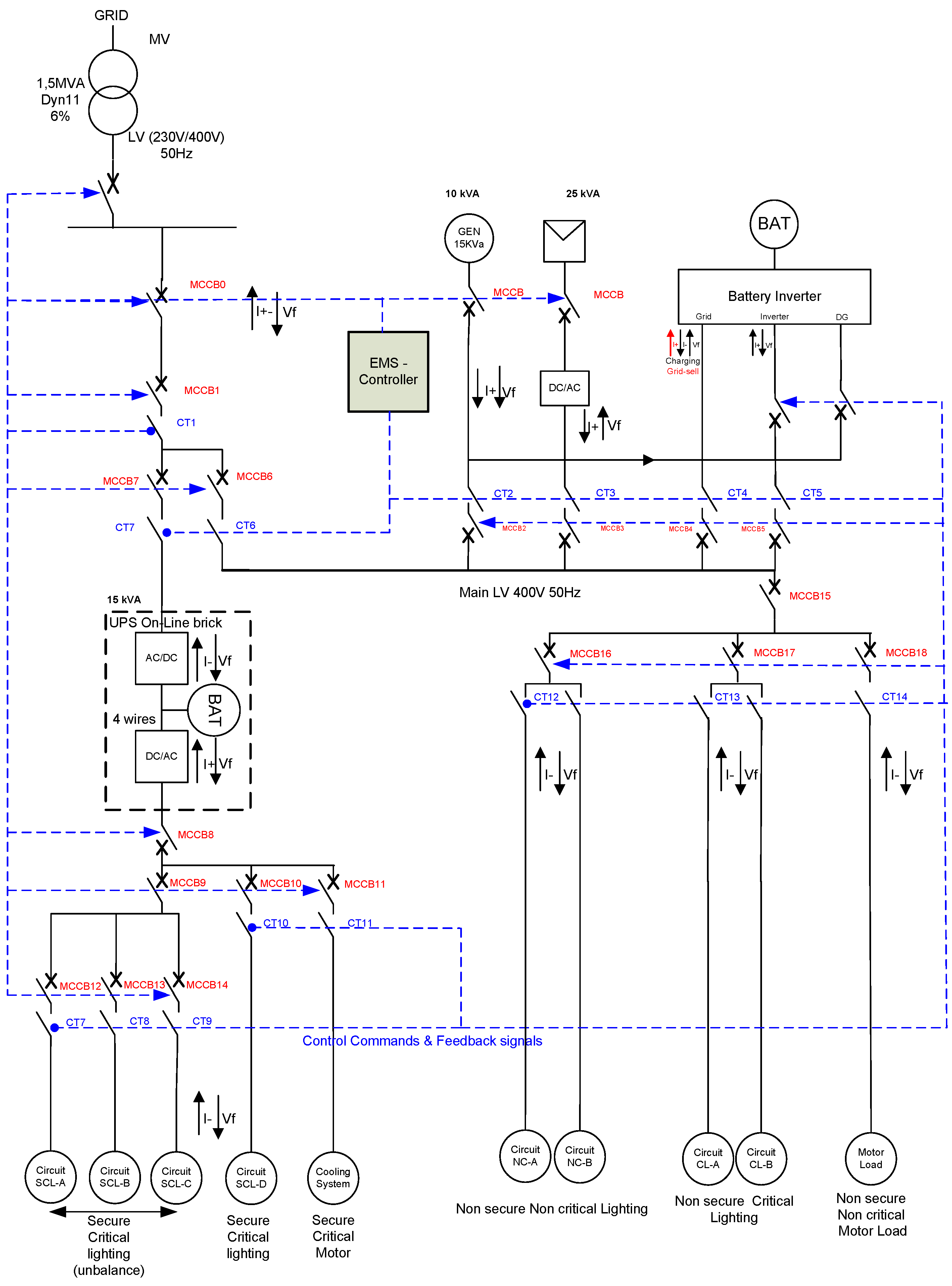
| Serial No. | Type of Source/Load | Specification |
|---|---|---|
| 1 | Total Network capacity | 100 kVA, 400 V, 3 PH, TT grounding system |
| 2 | PV Generator | 25 kW |
| 3 | Diesel Generator | 50 kW |
| 4 | BESS | 25 kW, 50 kWh |
| 5 | UPS | 15 kVA, 400 V, 3 PH |
| 6 | Managed Loads | 400 kVA, Air conditioner, Heater, & Standard 16 A Loads, 10 kVA |
| 7 | Priority unmanaged loads (Single phase) | PH 1-N 230 V, Lighting: 13 kVA, PF 0.7 & Loads: 12 kVA, PF 0.8 PH 2-N 230 V, Lighting: 8 kVA, PF 0.55 & Loads: 7 kVA, PF 0.6 PH 3-N 230 V, Lighting: 16 kVA, PF 0.8 & Loads: 3.5 kVA, PF 0.67 |
| 8 | Priority unmanaged loads (Three phase) | 400 V, 3 PH + N: 20 kVA, PF 0.85 (Motor Loads) |
| 9 | Critical unmanaged loads (Three phase) | 400 V, 3 PH + N: 6.45 kVA, PF 0.85 (Miscellaneous Loads) |
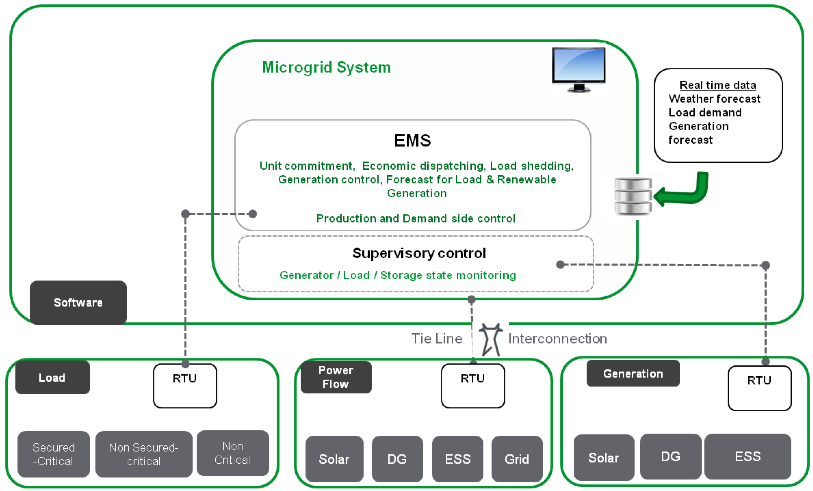
| Serial No. | Type | Description | Acquired Data to EMS | Control Command from EMS |
|---|---|---|---|---|
| 1 | Source | PV Generator | P, Q, I, V, F | P, Q |
| 2 | Source | BESS | V, I, SOC | Charge/Discharge |
| 3 | Source | DG | P, Q, I, V and Fuel level | P, Q |
| 4 | Load | Cooling | T, C, Occupancy | On/Off |
| 5 | Load | Lighting | L, Occupancy | On/Off |
| 6 | Load | Pump | Water level | On/Off |
| Cost of Energy | Grid Power | PV | State of UPS | UPS SOC | Battery Storage (BESS) | DG | Critical Secure Loads | Non-Secure & Critical Loads | Non-Secure & Non-Critical Loads |
|---|---|---|---|---|---|---|---|---|---|
| Low | Full | Share load & charge BESS | Online | Charge | Charge | Off | Grid | Grid | Grid |
| Medium | Partial | Share load & charge BESS | Online | Off | Supply | Off | Grid | Grid + BESS | Grid + BESS |
| High | Partial | Share load only | Online | Off | Supply | Off | UPS | BESS | Shed All loads |
| DES Availability | Grid Power | PV | State of UPS | UPS SOC | Battery Storage (BESS) | DG | Critical Secure Loads | Non-Secure, Critical Loads | Non-Secure, Non-Critical Loads |
|---|---|---|---|---|---|---|---|---|---|
| PV | Off | Share load & charge BESS | Serve Secure load | Dis charge | Charge | Off | UPS | PV | Shed all loads |
| PV and BESS | Off | Share load | Serve Secure load | Dis charge | Supply | Off | UPS | PV + BESS | Curtail |
| PV and DG | Off | Share load & charge BESS | Serve Secure load | Charge | Charge | ON | UPS | PV + DG | Curtail |
| Parameter | Limit | Value |
|---|---|---|
| Voltage limits and disconnection time | Under voltage LV1 Tripped value (V) | 195.5 V |
| Under voltage LV1 Tripping Time (s) | ≤2 s | |
| Over voltage LV2 Tripped value (V) | 310.5 V | |
| Over voltageLV2 Tripping Time (s) | ≤50 ms | |
| Under voltage LV2 Tripped value (V) | 195.5 V | |
| Under voltage LV2 Tripping Time (s) | ≤100 ms | |
| Over voltage LV1 Tripped value (V) | 253 V | |
| Over voltage LV1 Tripping Time (s) | ≤2 s | |
| Grid frequency limits and disconnection time | Under frequency LV1 Tripped value (Hz) | 49 Hz |
| Under frequency LV1 Tripping Time (s) | ≤200 ms | |
| Over frequency LV1 Tripped value (Hz) | 51 Hz | |
| Over frequency LV1 Tripping Time (s) | ≤200 ms | |
| Reconnection Time (s) | 20–300 s |
© 2017 by the authors. Licensee MDPI, Basel, Switzerland. This article is an open access article distributed under the terms and conditions of the Creative Commons Attribution (CC BY) license (http://creativecommons.org/licenses/by/4.0/).
Share and Cite
Ganesan, S.; Padmanaban, S.; Varadarajan, R.; Subramaniam, U.; Mihet-Popa, L. Study and Analysis of an Intelligent Microgrid Energy Management Solution with Distributed Energy Sources. Energies 2017, 10, 1419. https://doi.org/10.3390/en10091419
Ganesan S, Padmanaban S, Varadarajan R, Subramaniam U, Mihet-Popa L. Study and Analysis of an Intelligent Microgrid Energy Management Solution with Distributed Energy Sources. Energies. 2017; 10(9):1419. https://doi.org/10.3390/en10091419
Chicago/Turabian StyleGanesan, Swaminathan, Sanjeevikumar Padmanaban, Ramesh Varadarajan, Umashankar Subramaniam, and Lucian Mihet-Popa. 2017. "Study and Analysis of an Intelligent Microgrid Energy Management Solution with Distributed Energy Sources" Energies 10, no. 9: 1419. https://doi.org/10.3390/en10091419