Subsynchronous Torsional Interaction of Wind Farms with FSIG Wind Turbines Connected to LCC-HVDC Lines

1
Department of Electrical Engineering, North China Electric Power University, Baoding 071003, China
2
State Key Laboratory of Advanced Power Transmission Technology (Global Energy Interconnection Research Institute), Beijing 102209, China
*
Author to whom correspondence should be addressed.
Energies 2017, 10(9), 1435; https://doi.org/10.3390/en10091435
Submission received: 21 June 2017
/
Revised: 7 August 2017
/
Accepted: 14 September 2017
/
Published: 18 September 2017
(This article belongs to the Section F: Electrical Engineering)
Abstract
:High-voltage direct current (HVDC) lines with line-commutated converter (LCC) are being increasingly employed to transmit bulk wind power over long distance. However, this may cause the sub-synchronous torsional interaction (SSTI) between the wind farms and the LCC-HVDC system. The SSTI characteristics of wind farms with fixed-speed induction generator (FSIG) wind turbines connected to LCC-HVDC are investigated in this paper. To simplify the calculations, a modular modeling method is proposed for building the small-signal mathematical model of the investigated system. Small-signal analysis, participation factor analysis, and impact of dominant factors analysis are then applied to investigate the SSTI characteristics under different operating conditions. Three oscillation modes associated with the SSTI are identified in the entire system through small-signal and participation factor analysis, comprising two torsional modes and an electromechanical mode. Impact of dominant factors analysis shows that the system becomes less stable as the wind farm capacity grows and the distance between FSIG wind farm and the rectifier station increases. Moreover, the above analysis suggests that wind farms with FSIG connected to LCC-HVDC lines may not cause unstable SSTI. The electromagnetic transient simulations based on PSCAD/EMTDC (Power Systems Computer-Aided Design/Electromagnetic Transients including DC) verify these results.
1. Introduction
Due to the increasing energy demand and environmental issues, the number of wind farms is rapidly increasing in many countries [1,2,3]. At present, the most commonly employed wind turbine in the field of wind power generation are doubly-fed induction generator (DFIG) and direct-drive permanent-magnet synchronous generator (PMSG). Most of the newly constructed wind farms also employ more and more DFIG and PMSG, no longer adopting fixed-speed induction generators (FSIG). However, before the emergence of variable-speed wind turbine generators technology, FSIG were already widely used, and these FSIG-based wind farms are still in operation at present. Therefore, FSIG-based wind farms still have a certain percentage in the existing large-scale wind farms [3,4,5,6,7].
To implement the large-scale integration of wind energy supplies, series compensation in existing line, and building of new AC line and high-voltage direct current (HVDC) lines with line-commutated converter (LCC) are currently being considered. However, series compensation may potentially induce subsynchronous resonance (SSR) which can cause shaft failures [8]. SSR is an electromechanical oscillation caused by the coupling between generator and transmission system with series compensation capacitor [9]. Researches on SSR in FSIG-based wind farms, which is caused by series compensation, have been reported in the literatures. Reference [10] was the first paper to analyze the possibility of SSR in FSIG-based wind farms. The further analyses of SSR in single-cage and double-cage (FSIG) wind farms were presented in [6,11], respectively. It is shown in [6,10,11] that the SSR may happen in FSIG-based wind farms even at real levels of series compensation. In [12], the flexible AC transmissions system (FACTS) controllers, static var compensator (SVC) and thyristor controller series compensator (TCSC) were proposed to damp SSR in FSIG-based wind farms.
For the long-distance transmission of energy power, LCC-HVDC is a preferred option because of its high power control capability and fast modulation ability [13]. In China, three LCC-HVDC projects have been put in operation, and three projects are under construction, aiming to transmit wind power from west and north of China to east and south of China. A few LCC-HVDC projects in the United States are also planned to transmit wind power [7].
However, the applications of LCC-HVDC also bring new problems to the stability of power systems. Past experiences and studies have shown that fast response controller of LCC-HVDC may lead to subsynchronous torsional interaction (SSTI) in nearby steam turbine-generator (TG) [14,15]. SSTI is an electromechanical interaction between the TG shaft and the power electronic equipment (HVDC and FACTS) within the subsynchronous frequency range [1]. This problem may produce increased oscillations in the torsional modes of TG shaft. If proper commeasures are not considered, it can cause cumulative fatigue damage, which shortens the service lifespan of the TG shaft [16].
In 1977, the undesirable interaction between LCC-HVDC and the shaft of nearby steam TG was observed during the field tests on the Square Butte HVDC project [17]. It was the first SSTI event in engineering between LCC-HVDC and an electrical-closed steam TG. Since then, many technical papers have studied the cause and suppression measures for this oscillation. The research results showed that the fast-response constant current controller of the LCC-HVDC rectifier side may produce negative damping on near steam TG under certain conditions. When the damping of the whole system is negative, the natural torsional mode of the shaft can be excited, which leads to exponentially growing oscillation in the mechanical and electrical systems [1,18]. The subsynchronous damping controller (SSDC) was proposed by [8], and was widely used in practical engineering to provide positive damping over subsynchronous frequencies range [19,20].
In general, the shaft system of wind TG consists of hub and blades, shaft, gearbox, etc. [1]. Similar to that of steam TG, the shaft of wind TG also exhibits modes of mechanical oscillation, and its natural torsional frequencies usually lie within subsynchronous frequency range. When the wind TG is connected in the close vicinity of the LCC-HVDC system, LCC-HVDC may cause negative damping and excite the oscillation of shaft of wind TG under some operational conditions. Then this oscillation will lead to the SSTI between LCC-HVDC and wind TG, which threatens the safe operation of wind farms.
The SSTI between DFIG wind farms and LCC-HVDC was analyzed by small-signal methods and electromagnetic transient (EMT) simulations in [3]. However, this method has to refer all nonlinear equations and eliminate some differential equations to describe the entire system. What is more, when the system structure undergoes changes, resulting in changes in the state variables, the small-signal model of the system must be reestablished thoroughly. The SSTI behavior between FSIG-based wind farms and LCC-HVDC was first analyzed through EMT simulations in [18], but the mechanism was not analyzed. The SSTI behavior of FSIG farms that connected to LCC-HVDC and series compensated line simultaneously was analyzed in [7]. However, the wind turbine generator’s (WTG) drive train adopts the two-mass model, the subsynchronous oscillation mode may not be observed. Moreover, little information was reported in the literature on a systematic analysis of SSTI in FSIG-based wind farms connected only to LCC-HVDC.
In China, most of power energy generated from FSIG-based wind farms is transmitted by LCC-HVDC. From the above analysis, there is a possibility of SSTI between LCC-HVDC and shaft of these FSIG-based wind farms under some certain conditions. This raises a question: whether this SSTI will cause the unstable operation of wind farms and LCC-HVDC, and what is the characteristic of this type of SSTI? The operators of FSIG-based wind farms and power grid are very concerned about this phenomenon. However, the current research on this aspect is very limited and cannot provide enough information. Aiming at this engineering issue, this paper focuses on SSTI between LCC-HVDC and FSIG-based wind farms. The characteristic of this type of SSTI is investigated in detail, by the methods of small-signal analysis and EMT simulations.
The contributions of this work are shown as below: (1) a typical three-mass model of FSIG-based wind farms connected to LCC-HVDC lines is built. (2) To simplify calculations, a modular modeling method is proposed for building the small-signal mathematical model of the investigated system. When the system structure undergoes changes, resulting in changes in the state variables, the small-signal model only needs to be changed slightly. (3) The characteristics of SSTI in FSIG connected to LCC-HVDC are explored. (4) The impact of dominant factors analysis is conducted, including mechanical parameters, wind farm capacity, controller parameters, and the distance between the rectifier side of LCC-HVDC and wind farms. The results of this paper build the foundation to improve the stability level of FSIG-based wind farms connected to LCC-HVDC.
The remainder of this paper is structured as below. In Section 2, the modeling of the whole system is established. Small-signal analysis and participation factor analysis are utilized to characterize SSTI in Section 3. Section 4 describes the impact of dominant factors analysis for the investigated system. The results of the small-signal analysis are validated by the simulations in Section 5. Section 6 discusses the risks of potentially unstable SSTI phenomenon for systems with wind farms-based FSIG wind turbines connected to LCC-HVDC lines. Section 7 summarizes the paper.
2. System Modeling
The investigated system, given in Figure 1, comprises FSIG-based wind farm with 500 WTGs, an equivalent AC system S1 and a LCC-HVDC lines. It is assumed that the FSIG-based wind farm is an aggregation by many 750 kW single-cage squirrel cage IGs. The wind speed is assumed to be 12 m/s. The rated voltage of each induction generator is 0.69 kV. This assumption adopts the weighted admittance averaging method supported by several recent studies [6,21,22,23]. Those studies indicate that this simplification is able to offer a reasonable equivalent model for SSTI stability research. The parameters of the IG given in Appendix A, Table A1, are provided by actual wind farms in Northwest China.
The AC system is modeled as an equivalent voltage source S1 and a series impedance RS + jXS. The LCC-HVDC transmission line is derived from the CIGRE (International Council on Large Electric systems) HVDC benchmark model [24]. The rated LCC-HVDC transmission power is 1000 MW and the transmission voltage level is 500 kV. Other parameters are given in Appendix A, Table A2 and Table A3. The system with those parameters is hereafter named the Base case in this paper.
The system consists of four parts: (i) the shaft system, (ii) the induction generator (IG), (iii) the LCC-HVDC transmission line, (iv) the AC network. The mathematical modeling of each part is shown as follows.
2.1. Modeling of the Shaft System
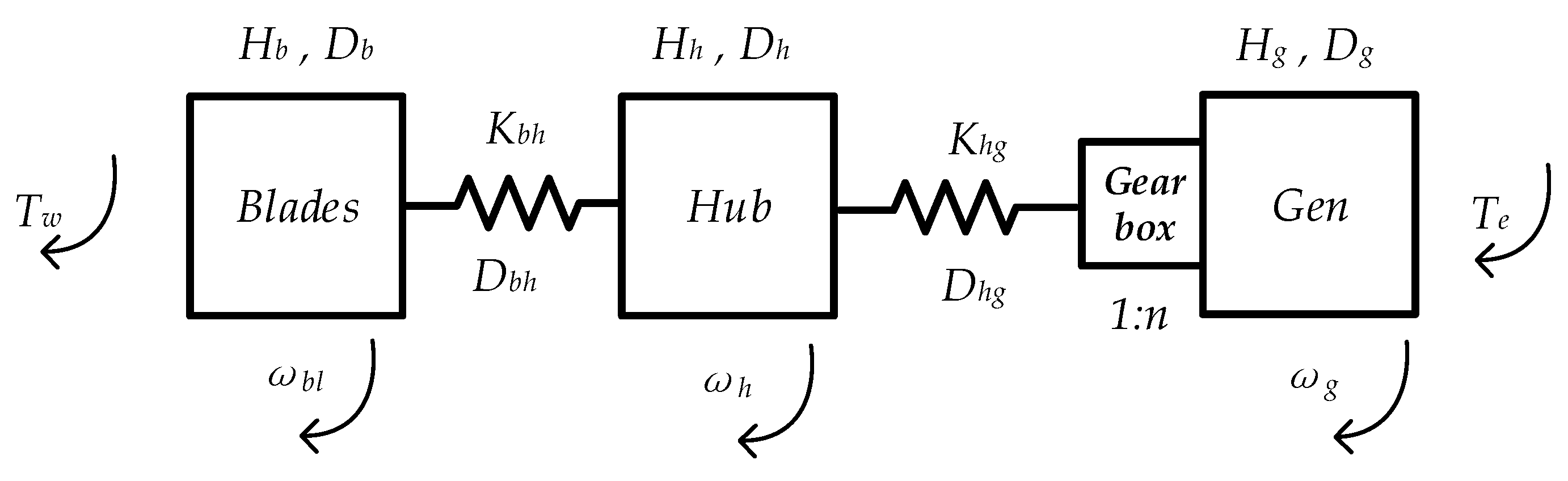
Generally speaking, the shaft system of a wind turbine generator consists of hub and blades, low-speed shaft, gearbox, high-speed shaft and generator rotor [18]. In this paper, it is represented as a three-masses spring system in Figure 2 [12]. The first two masses represent the blades and the hub, respectively; the third mass represents the gearbox and the generator.
The dynamic equations of this mass-spring system can be expressed as:
where:
- Tw: wind turbine torque;
- Te: generator torque;
- Hb, Hh, Hg: inertia of blades, hub and generator, respectively;
- Db, Dh, Dg: self-damping of blades, hub and generator respectively;
- Dbh: mutual damping between blades and hub;
- Dhg: mutual damping between hub and generator;
- ωb: Synchronous angular frequency;
- ωbl, ωh, ωg: rotational speed of blades, hub and generator respectively;
- Kbh: spring constants between blades and hub;
- Khg: spring constants between hub and generator.
The parameters of the mass-spring model of the turbine generator system are listed in Table 1 [12]. For the system here investigated, we assume zero damping coefficients for all self-damping and mutual damping. According to [12], the torsional natural frequencies of this system calculated for the mass spring turbine generator are 0.609 Hz and 4.982 Hz.
2.2. Modeling of the Induction Generator
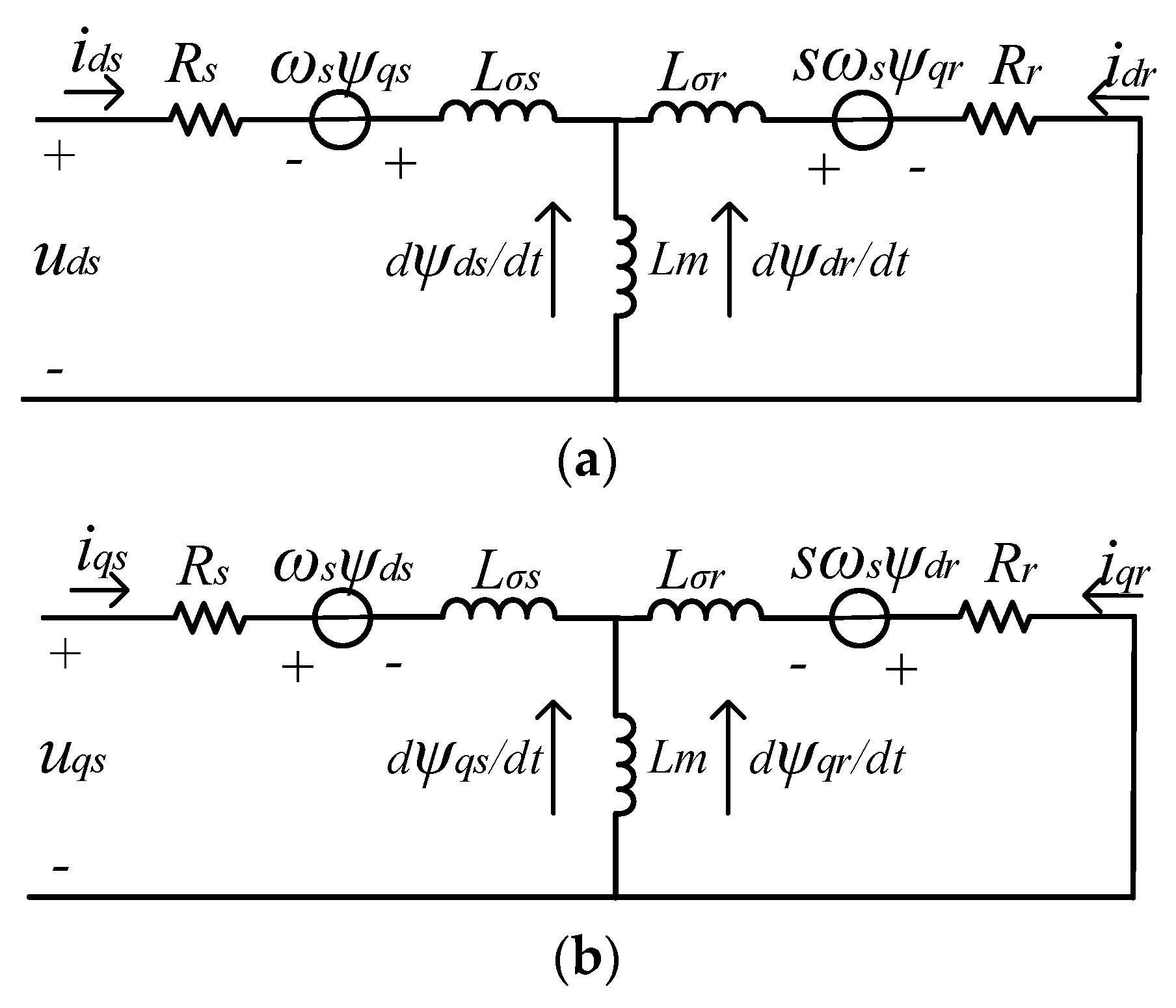
Figure 3 shows the equivalent circuit of a squirrel cage IG with a shunt capacitor. Shunt capacitor CF is employed to provide the reactive power consumption for the FSIG-based wind turbine, as they do not include an internal excitation system. A detailed mathematical model of a single-cage IG in a d-q reference frame is given by Equation (3).
The electromagnetic torque is expressed as:
where:
- Rs, Rr: Resistance of stator and rotor, respectively;
- Xm: Excitation reactance;
- Xsσ, Xrσ: Leakage inductance of stator and rotor, respectively;
- Te: Electromagnetic torque.
2.3. Modeling of the LCC-HVDC Lines
The LCC-HVDC system is adopted from the CIGRE HVDC model. Figure 1 shows its typical configuration. Constant direct current and constant extinction angle control are employed on rectifier and inverter side, respectively.
The differential equations of the DC transmission line are written in Equation (6).
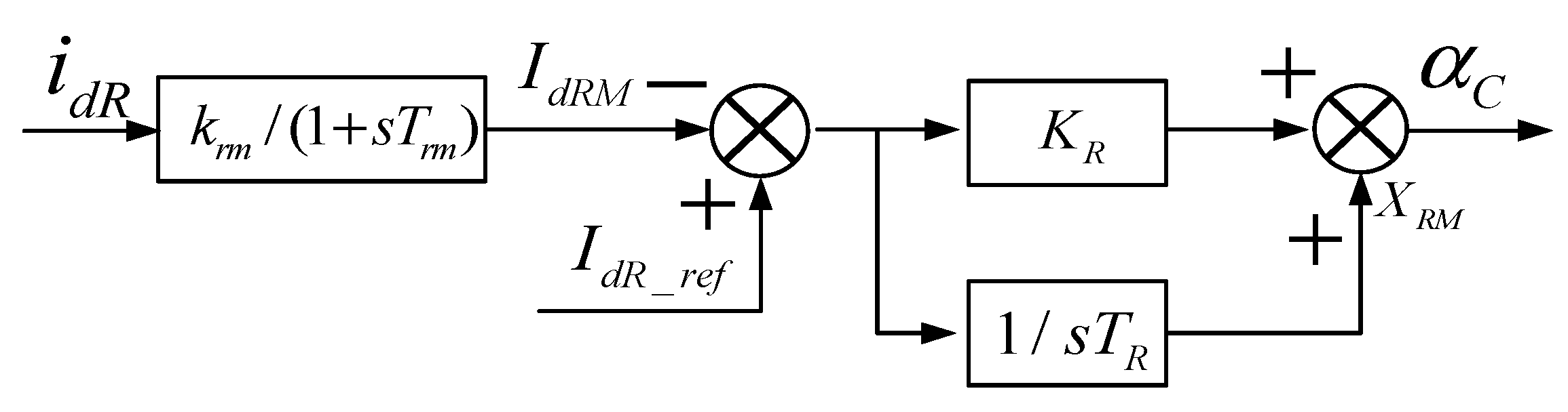
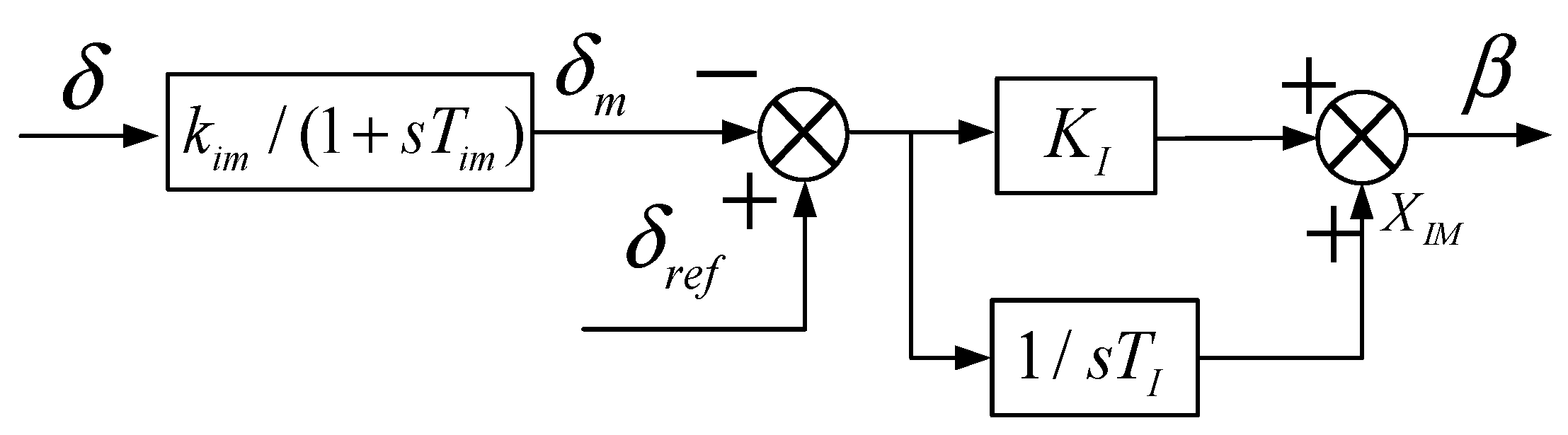
The block diagrams of rectifier and inverter control are given in Figure 4 and Figure 5, respectively. The differential equations of both sides are listed as Equations (7) and (8), respectively.
- UdR, UdI: DC bus voltages of rectifier and inverter station, respectively;
- IdR, IdI: DC current injected from the rectifier and absorbed by the inverter;
- Rd, Ld, Cd: DC line resistance, DC line inductance and DC-link capacitance, respectively;
- UCd: DC-link capacitor voltage.
- Krm, Trm: the gain and time constant of DC current measurement, respectively;
- IdRM, Iref: the measured DC current of rectifier and the reference dc current, respectively;
- KR, TR: the gain and time constant of proportion integration (PI) controller in rectifier current controller;
- α: the reference firing angle of rectifier side;
- δ: the extinction angle of inverter side.
2.4. Modeling of the AC Network
The AC network comprises the equivalent voltage source S1, the reactive compensation capacitor CF, the AC shunt filter CB, and the AC transmission line, represented by resistance and inductance.
A general mathematical description of the capacitor and the transmission line are as follows: Capacitor:
Transmission line:
2.5. State-Space Model of the Entire System
The conventional method for small-signal analysis has to refer all nonlinear equations and eliminate some differential equations to describe the entire system. A drawback of this method is the large amount of calculation required, especially when the investigated system is complex. In order to simplify the calculation, modular modeling method is proposed to build the small-signal model of the investigated system. Taking the capacitor of the AC system as an example, the procedures for modular modeling method are as follows
Step 1. Model linearization
The nonlinear equations describing the subsystems, given in Section 2, are expressed in the form of Equation (11)
To study the system stability after suffering a small disturbance, it is necessary to build the linear model of the subsystem around the equilibrium point [25]. For the equilibrium point , the Equation (11) can be written as:
where:
- : the initial state vector;
- : the initial input vector.
After subjecting to small perturbations, the initial state vector x and the input vector u can be expressed by:
The new state must satisfy Equation (11). Hence,
The functions Equation (11) can be expressed in the form of Taylor’s series expansion. Assuming the perturbation is small enough, the second- and higher-order powers can be neglected. The Equation (14) can be expressed as:
Since Equation (12), the linearization result is obtained.
For the capacitor of the AC system, the linear equations can be written as:
Step 2. Small-signal model of subsystems
Based on the linear subsystems model as outlined in Step 1, the linear equations can be expressed in the form of the small-signal model. The state-space of a subsystem frame is given as:
where x is the state variable of the subsystem, u is the input variable, y is the output variable, A, B, C and D are all constant matrices. According to Equation (16), the A, B can be expressed as,
C, D are determined by the output variable y of the subsystem.
For the capacitor of the AC system, Δuc is the state variable and the output variable, Δic is the input variable. The state-space of the capacitor of the AC system can be written as:
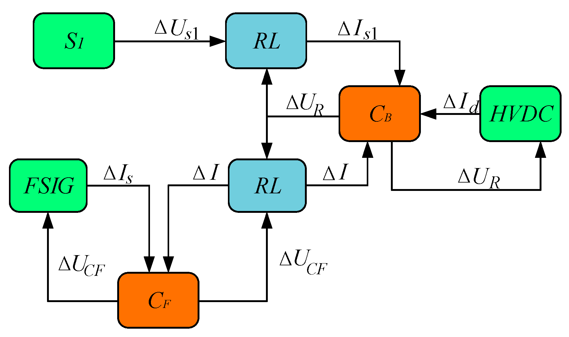
Other subsystems have similar format. After determining the inputs and outputs of each module, the state-space model of each subsystem can be obtained. The input and output variables of every module are given in Figure 6, which is also the interface between the modules.
Step 3. Modeling of the entire system
All subsystems described above are integrated, and the small-signal model for the entire system is developed through input/output interface and MATLAB function ‘linmod’ automatically.
The modular modeling method only requires the small-signal model of subsystems. The elimination process of the differential equations is automatically performed in MATLAB. In comparison with conventional methods, the modular modeling method requires a reduced amount of calculations and is less prone to errors.
3. Subsynchronous Torsional Interaction Analysis
Based on the linearized small-signal model presented in Section 2, small-signal analysis and participation factor analysis are performed to investigate the SSTI of the system under study.
3.1. Small-Signal Analysis
The small-signal model of the entire system as derived in Section 2 can be described as:
where is the coefficient matrix of the study system. The characteristic equation of the coefficient matrix is expressed in the form of Equation (23).
The state matrix A results in n eigenvalues. The system eigenvalues of the Base case are calculated with MATLAB using the small-signal model. There are 25 state variables, resulting in 25 eigenvalues. The modes associated with SSTI are shown in Table 2.
The frequencies of the three modes are 4.982 Hz, 3.219 Hz and 0.187 Hz, respectively. Other modes with high oscillation frequencies are not considered for the SSTI analysis as they are strongly damped. As shown in Table 2, real parts of the three modes associated with SSTI are negative. Therefore, the system of the Base case eventually settles down after suffering a small disturbance.
3.2. Participation Factor Analysis
Based on the small-signal analysis results, the influence of different state variables on the modes associated with SSTI is studied through the participation factor analysis. The participation factor can reflect the relative contribution of a given state variable to the modes. For a system with n eigenvalues, it is defined as:
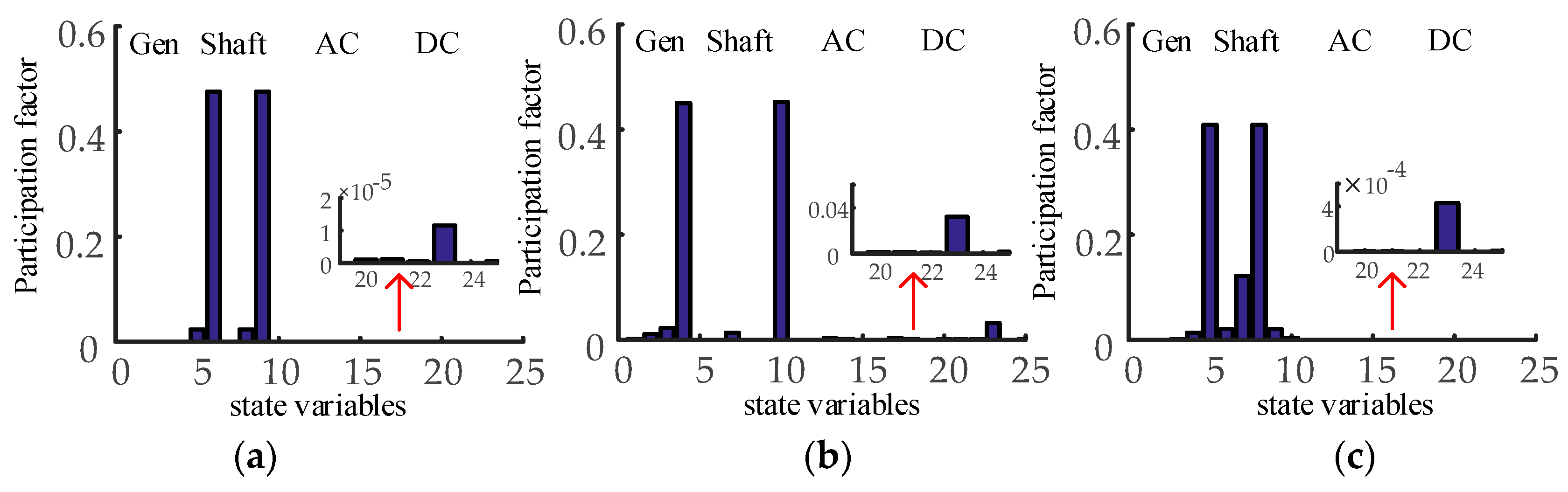
where Uki and Vki are the k-th elements of the left and right eigenvectors associated with the i-th mode, respectively. The state variables of the entire system are given in Table 3. Figure 5 shows participation factor of the main oscillation modes.
Figure 7a shows the participation factors for the Mode-1. It is highly sensitive to the shaft state variables, especially ωh and δh. Other state variables have a small influence on this mode. The oscillation frequency of Mode-1 is 4.982 Hz, which is the same as the torsional natural frequency of 4.982 Hz, and thus it is named as Torsional-1 mode (Tor-1 mode for short).
Figure 7b shows the participation factors for the Mode-2. It is affected by the state variables of the shaft and also of the generator, especially ψdr and δg. The variations of torsional and electrical parameters have a great influence on this mode, which is considered as an Electromechanical mode (Electro mode for short).
Figure 7c gives the participation factors for the Mode-3. It is mainly affected by the state variables of the shaft. Also, the rotor flux ψr has a slight effect on this mode, and as a consequence the changes in electrical parameters have an effect on this mode. However, this effect is small if compared to the electromagnetic mode. This mode is another torsional natural mode, with an oscillation frequency of 0.187 Hz. It is then called Torsional-2 mode (Tor-2 mode for short).
4. Impact of Dominant Factors on SSTI
In order to investigate the SSTI characteristics, we carry out in this section an analysis of the impact of dominant factors, including mechanical parameters, wind farm capacity, controller parameters and distance between FSIG-based wind farm and the rectifier station of LCC-HVDC.
4.1. Impact of Mechanical Parameters
The effect of inertia constants (Hb, Hh, Hg) and the spring constants (Kbh, Khg) on the oscillation modes are described in this section. Due to space limitations, only three cases are compared to investigate the SSTI characteristics. Table 4 and Table 5 show the variations of the damping ratio and oscillating frequency of the main oscillation modes resulting from the parameter changes. The damping ratio is given as follows:
where λ = σ + jω. The damping ratio ξ indicates the attenuation rate of the oscillation mode. The larger ξ is, the faster the oscillation decays.
As shown in Table 4, Hb mainly affects the Tor-2 mode. When Hb increases, the frequency of Tor-2 mode decreases and the damping ratio increases. Hh has an effect on Tor-1 mode. When Hh increases, the frequency of the Tor-1 mode reduces and the damping ratio increases. Hg mainly affects the Electro mode. If Hg increases, the frequency of the Electro mode decreases, and the damping ratio increases.
As shown in Table 5, Kbh mainly affects the Tor-1 mode. As the Kbh increases, the frequency of Tor-1 mode increases and the damping ratio decreases. Khg has an effect on the Tor-2 mode. Along with the increase of Khg, the frequency of the Tor-2 mode is reduced and the damping ratio increases. Both Kbh and Khg have little effect on the electromechanical mode.
The data analysis results are summarized as follows: the Tor-1 mode is very sensitive to Hh and Kbh. The Electro mode is sensitive to Hg. The Tor-2 mode is sensitive to Hb, and Khg. Therefore, an appropriate design of the mechanical parameters can help avoid some resonances and enhance the damping.
4.2. Impact of Wind Farm Capacity
The impact of wind farm capacity is now examined for the system under investigation. The number of the WTG is varied from 100 to 500, and the power of HVDC line is 1000 MW. Its impact on the system is examined by analyzing the eigenvalues of the three modes associated with SSTI, as depicted in Figure 8.
As shown in Figure 8, the wind farm capacity has a small effect on the frequency of the torsional modes. With the increase of the farm capacity, the oscillation frequency of the Electro mode decreases, and the damping of the three modes also decreases. Under this condition, the system becomes less stable if the wind farm capacity increases. However, since all three modes have a negative real part, the system does not experience unstable SSTI phenomenon within the range of variation considered here.
4.3. Impact of Controller Parameters KR and TR
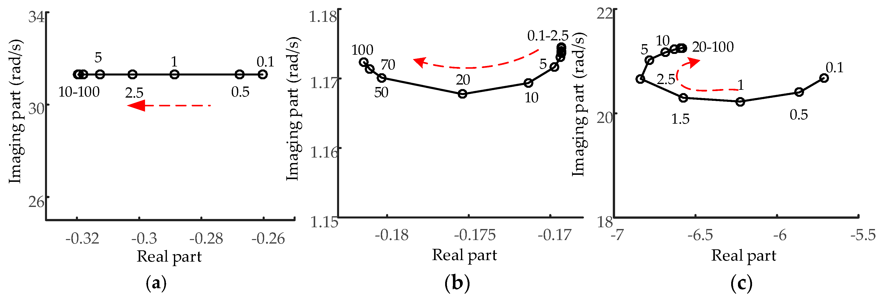
Conventional thermal power sent out via LCC-HVDC transmission lines may potentially cause subsynchronous oscillation. In most cases it is related to the current controller of the rectifier station. In this section, the controller parameters at the rectifier side are considered for the SSTI analysis. The controller gain KR and TR are now changed from 0.1 to 100 respectively, and their nominal value is 1.0989 and 0.01092, respectively. Other parameters remain unchanged.
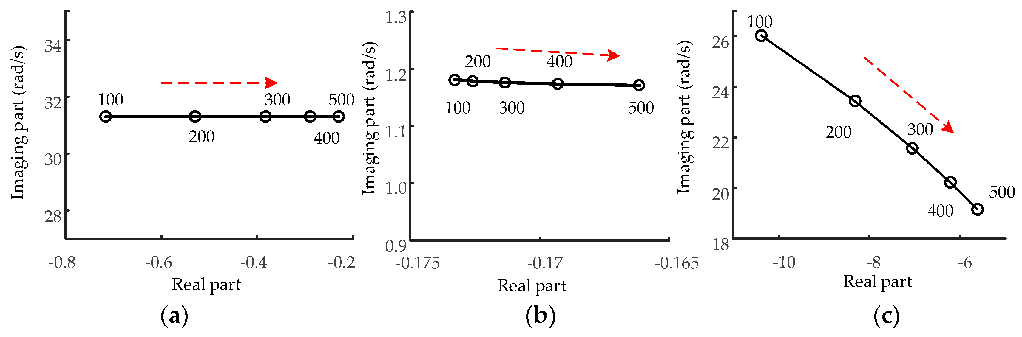
As KR increases, the eigenvalues of Tor-1 and Tor-2 mode move toward the right and become less stable, as shown in Figure 9a,b. The frequencies of the two modes do not change. Figure 9c shows that the Electro mode becomes less stable and its oscillation frequency changes within narrow range. The results demonstrate that the damping of the system decreases when KR increases.
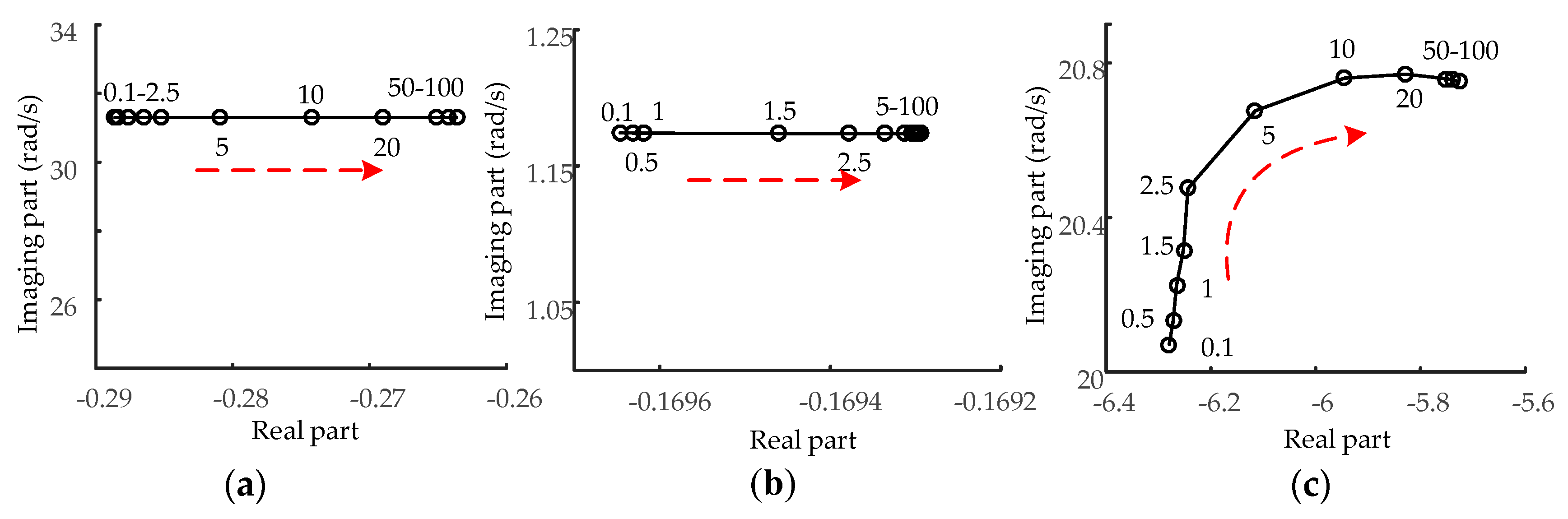
As TR increases, both the Tor-1 mode and Tor-2 mode vary in a narrow band, as shown in Figure 10a,b. The Electro mode eigenvalues move left until the time constant reaches 2.5TR, and then return toward the right. The oscillating frequency of the Electro mode keeps increasing after 2.5TR while the time constant increases, as seen in Figure 10c.
All eigenvalues have a negative part, which indicates that the system has positive damping. Therefore, the system here investigated does not undergo unstable SSTI phenomenon within the range of variation of KR and TR.
4.4. Impact of Distance between Wind Farm and Rectifier Station
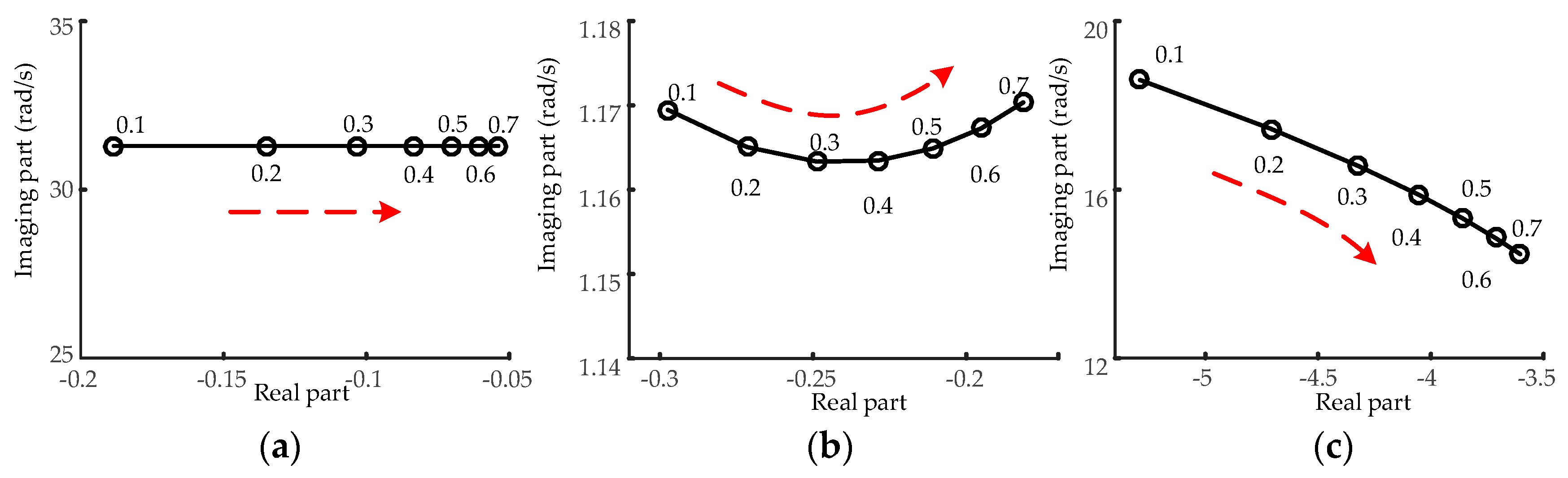
The distance between the rectifier station of LCC-HVDC and the wind farm is changed by adjusting the parameter of the impedance of the line Xl, as shown in Figure 1. The line impedance is varied between 0.1 p.u and 0.7 p.u.
Figure 11 shows its impact on the oscillatory modes. When the distance increases, all the oscillation modes become less stable. The oscillation frequency of the Electro mode decreases, while the oscillation frequency of the Tor-1 mode remains unchanged. Changes in all modes indicate that the system becomes less stable as the distance between the rectifier station and the wind farm increases.
5. Electromagnetic Transient Simulation Verification
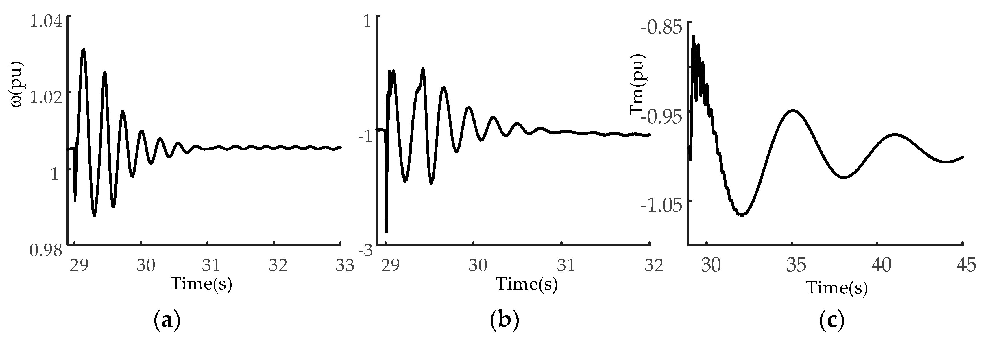
To validate the results of Section 3 and Section 4, electromagnetic transient simulations of the nonlinear system were conducted in PSCAD/EMTDC. The system and the controller parameters are the same as in the small-signal linearized model. A three-phase ground fault is simulated at the rectifier station shown in Figure 1, which is started t = 29 s and cleared after 0.075 s. The rotational speed ω, electromagnetic torque Te and mechanical torque Tm are observed.
5.1. Verification of Small-Signal Model
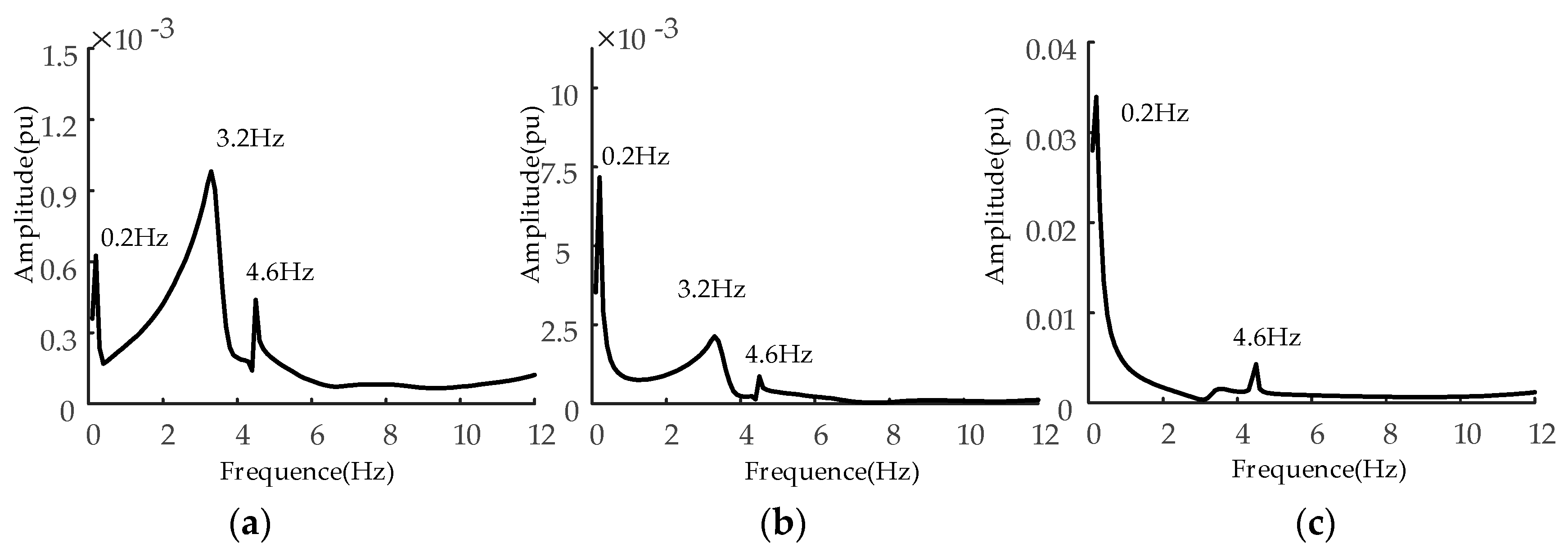
Figure 12 and Figure 13 illustrate the waveform and Fast Fourier Transformation (FFT) frequency spectrum of ω, Te and Tm for the Base case, respectively. As shown in Figure 12, the ω, Te and Tm eventually settle down after suffering this fault. This agrees with the small signal results listed of Table 2, where all eigenvalues have a negative part. As shown in Figure 13a,b, rotational speed and electromagnetic torque disturbance are contributed by the Tor-1 mode, Electro mode and Tor-2 mode. The modal frequencies obtained from spectrum analysis closely match the eigenvalue analysis given in Table 2. The frequencies obtained from spectrum analysis are 0.2 Hz (1.257 rad/s), 3.219 Hz 20.226 rad/s), and 4.6 Hz (28.902 rad/s), while the frequencies of the eigenvalues shown in Table 2 for the Base case are 0.187 Hz (1.175 rad/s), 3.2 Hz (20.106 rad/s) and 4.98 Hz (31.304 rad/s), respectively. Mechanical torque is contributed only by the torsional modes, as shown Figure 13c. Therefore, the results of electromagnetic transient simulation in this part confirm the accuracy of the small-signal analysis.
5.2. Impact of the Wind Farm Capacity
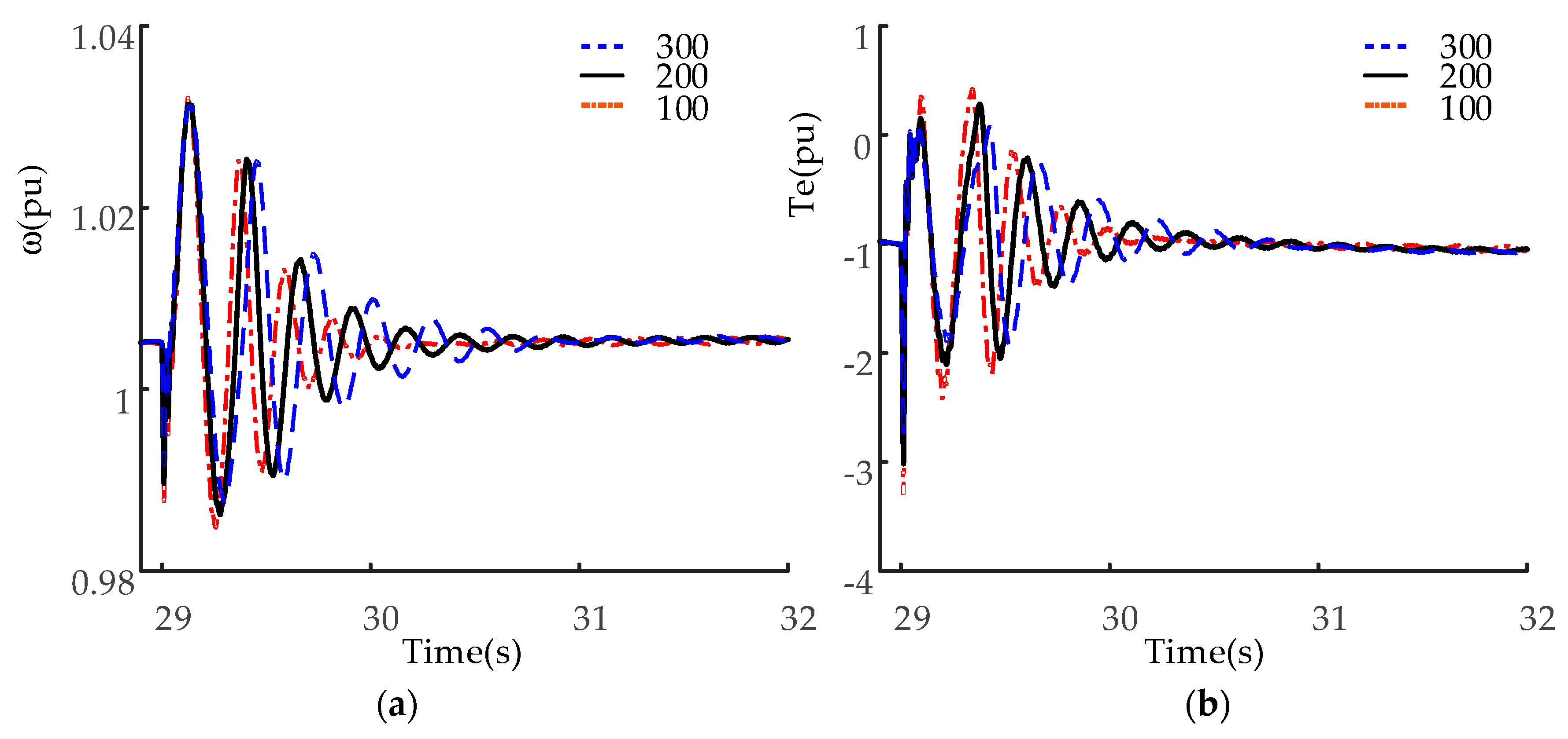
The small-signal analysis of the impacts of the wind farm capacity was also validated by the electromagnetic transient simulation. Figure 14 shows the rotational speed ω and electromagnetic torque Te for wind farms with capacities of 100, 200 and 300 WTGs, respectively.
As shown in Figure 14a, both rotational speed ω and electromagnetic torque Te oscillations were damped, and the system remained stable after a three-phase ground fault at the rectifier side. This also agrees with the results in Section 4.2, where all eigenvalues have a negative part. It also indicates that the system here investigated does not undergo unstable SSTI phenomenon within the tested range of parameters variation.
Meanwhile, the damping of the modes decreases as the capacity of the wind farm increases. As shown in Figure 14, the rotational speed ω and electromagnetic torque Te require a longer time to restore the stability with the increase of wind farm capacity. The simulation results are in good agreement with the results of the small-signal analysis described in Section 4.2.
5.3. Impact of the Mechanical Parameters
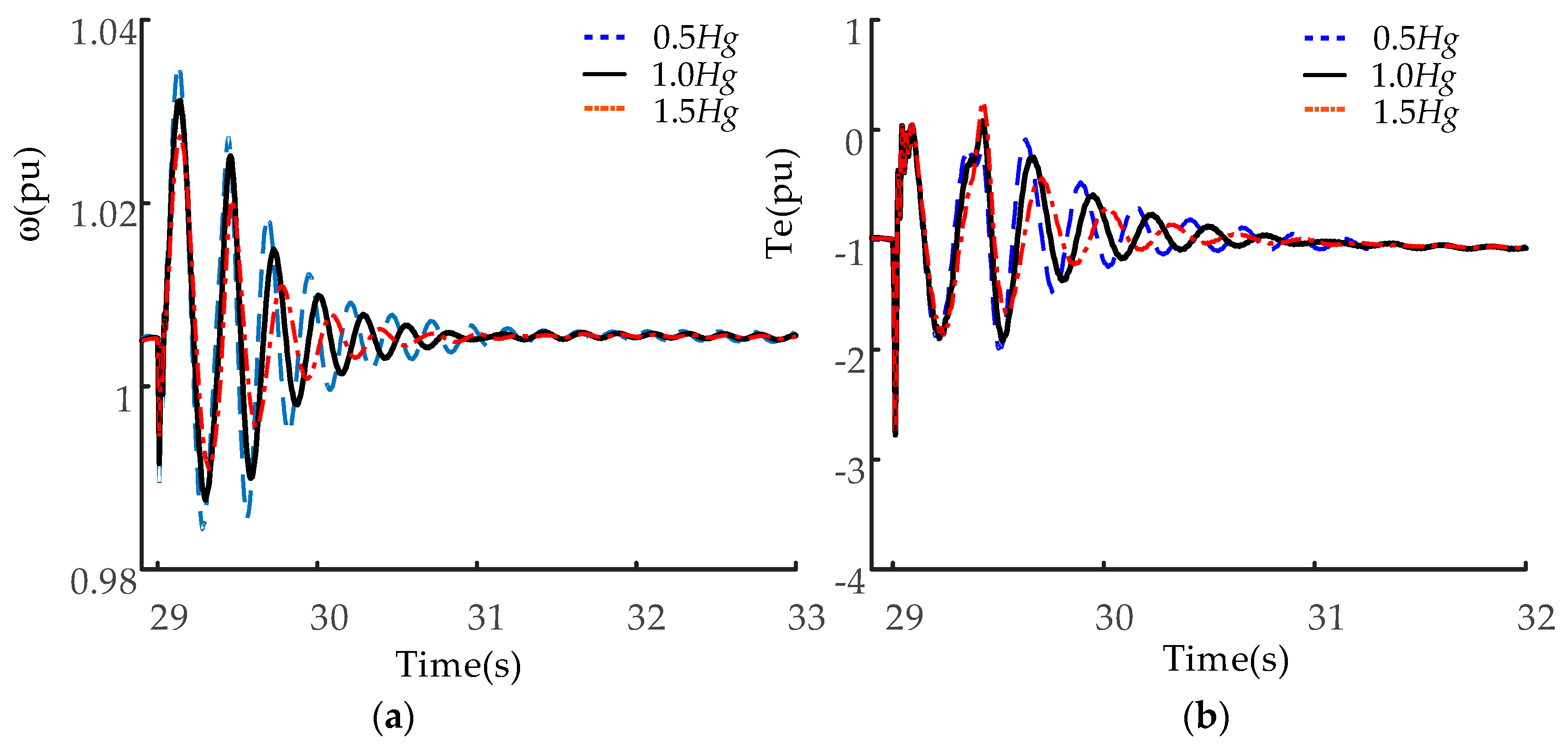
The small-signal analysis of the impacts of the mechanical parameters was also validated by the electromagnetic transient simulation. The rotational speed ω and electromagnetic torque Te with the effect of inertia constants Hg and the spring constants Khg are shown in Figure 15 and Figure 16, respectively.
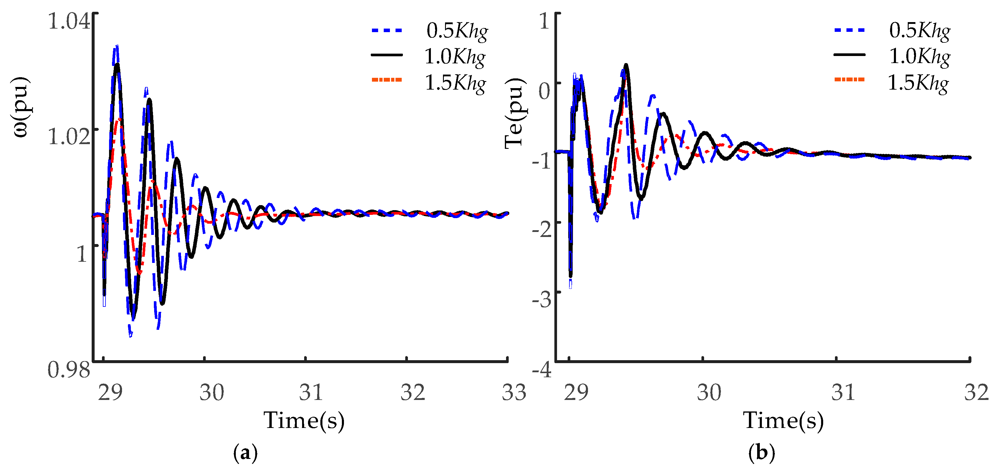
As it can be seen from Figure 15, when the inertia constants Hg increase, both the damping of the rotational speed ω and the electromagnetic torque Te will increase and have less oscillation. The system here investigated remains stable within the tested range of parameters variation due to the stable oscillation modes associated with SSTI. The simulation results are in good agreement with the results of the small-signal analysis described in Table 4. The simulation verifications analysis of the spring constants Khg has similar results shown in Figure 16.
The effects of other parameter changes on the SSTI were also studied by the electromagnetic transient simulations. The results, not shown here because of space limitations, also confirm the small-signal analysis of Section 4.
6. Risks Analysis of SSTI in FSIG-Based Wind Farms Connected to LCC-HVDC Lines
Based on the system studies described in this paper, risks analysis of SSTI for the study system is discussed in this section. The small-signal analysis in Section 3 indicates that the FSIG-based wind farms connected to LCC-HVDC lines could cause SSTI oscillation modes. There would be SSTI phenomenon for such system. However, even ignoring the shaft damping coefficients, the three oscillation modes still have negative real parts within the considered range of variation. Moreover, when the shaft damping of actual systems is taken into account, the overall positive damping will still be large. The dominant factors analysis in Section 4 also revealed that the system has positive damping under different operating conditions. The simulations in Section 5 show that the oscillation eventually is damped out after a short time period, even for the most severe three-phase ground fault disturbances.
Both small-signal analysis and electromagnetic transient simulations show that wind farms with FSIG connected to LCC-HVDC lines do not generate SSTI instabilities. Therefore, it is not necessary to plan a subsynchronous damping controller (SSDC) for real systems.
7. Conclusions
In this paper, a detailed SSTI analysis was carried out for a FSIG-based wind farm connected to LCC-HVDC lines. A comprehensive small-signal mathematical model was established by modular modeling method. Three main oscillation modes associated with SSTI were identified in the entire system by small-signal analysis, including two torsional modes and an electromechanical mode. The dominant factors analysis demonstrated that a system with a higher wind farm capacity or a longer distance between the wind farm and the rectifier station is more susceptible to drive the system less stable. The results indicate that wind farms with FSIG-based connected to LCC-HVDC lines may not induce unstable SSTI phenomenon. In addition, the results were verified by electromagnetic transient simulations in PSCAD/EMTDC. The analysis results of this paper offer the foundation for future study of the stability in wind farms with FSIG wind turbines connected to LCC-HVDC.
Acknowledgments
The authors thank the anonymous referees for their helpful comments and suggestions. This work was supported in part by Colleges and Universities in Hebei Province Science and Technology Research (grant numbers: Z2015041), in part by the State Key Laboratory of Advanced Power Transmission Technology (Grant No. GEIRI-SKL-2017-003).
Author Contributions
Benfeng Gao performed the literature review and established the small-signal mathematical model of the system. Ruixue Zhang performed the electromagnetic time-domain simulations in the PSCAD/EMTDC. Ren Li and Ruixue Zhang analyzed the data; Benfeng Gao and Ruixue Zhang wrote the paper. Hongyang Yu and Guoliang Zhao provided the wind farm data.
Conflicts of Interest
The authors declare no conflict of interest.
Appendix A

Table A1.
HVDC transmission system.
| Parameters (pu) | |||
|---|---|---|---|
| KR | 1.0989 | nR | 1.0165 |
| TR | 0.01092 | nI | 0.9963 |
| KI | 0.7506 | XCR | 0.1251 |
| TI | 0.0544 | XCI | 0.0567 |
| Kmr | 0.5 | Rd | 0.0088 |
| Tmr | 0.0012 | Ld | 0.7933 |
| Tmi | 0.002 | Cd | 2.7798 |
Table A2.
Induction generator.
| Parameters | |||
|---|---|---|---|
| Vs | 0.69 kV | Pg | 750 KW |
| Rs | 0.0103 Ω | ωs | 314.15 rad/s |
| Rr | 0.01718 Ω | Xsσ | 0.11 Ω |
| Xm | 7.8 Ω | Xrσ | 0.124 Ω |
Table A3.
AC network.
| Parameters (pu) | |
|---|---|
| Re | 0 |
| Xe | 0.14 |
| RS1 | 0.0225 |
| XS1 | 0.424 |
| CR | 0.4015 |
References
- Leon, A.E.; Solsona, J.A. Sub-synchronous interaction damping control for DFIG wind turbines. IEEE Trans. Power Syst. 2015, 30, 419–428. [Google Scholar] [CrossRef]
- Wang, L.; Xie, X.; Jiang, Q.; Liu, H.; Li, Y.; Liu, H. Investigation of SSR in practical DFIG-based wind farms connected to a series-compensated power system. IEEE Trans. Power Syst. 2015, 30, 2772–2779. [Google Scholar] [CrossRef]
- Yang, L.; Xiao, X.N.; Pang, C.Z. Oscillation analysis of a DFIG-based wind farm interfaced with LCC-HVDC. Sci. China Technol. Sci. 2014, 57, 2453–2465. [Google Scholar] [CrossRef]
- Yao, J.; Guo, L.; Zhou, T.; Xu, D.; Liu, R. Capacity configuration and coordinated operation of a hybrid wind farm with FSIG-based and PMSG-based wind farms during grid faults. IEEE Trans. Energy Convers. 2017, 32, 1188–1199. [Google Scholar] [CrossRef]
- Liu, J.; Chu, C. Long-Term voltage instability detections of multiple Fixed-Speed induction generators in distribution networks using synchrophasors. In Proceedings of the Power and Energy Society General Meeting (PESGM), Boston, MA, USA, 17–21 July 2016. [Google Scholar]
- Varma, R.K.; Moharana, A. SSR in double-cage induction generator-based wind farm connected to series-compensated transmission line. IEEE Trans. Power Syst. 2013, 28, 2573–2583. [Google Scholar] [CrossRef]
- Moharana, A.; Varma, R.K.; Seethapathy, R. Modal analysis of induction generator based wind farm connected to series-compensated transmission line and line commutated converter high-voltage DC transmission line. Electr. Power Compon. Syst. 2014, 42, 612–628. [Google Scholar] [CrossRef]
- Fan, L.; Kavasseri, R.; Miao, Z.L. Modeling of DFIG-based wind farms for SSR analysis. IEEE Trans. Power Deliv. 2010, 25, 2073–2082. [Google Scholar] [CrossRef]
- Livermore, L.; Ugalde-Loo, C.E.; Mu, Q.; Liang, J.; Ekanayake, J.B.; Jenkins, N. Damping of subsynchronous resonance using a voltage source converter-based high-voltage direct-current link in a series-compensated Great Britain transmission network. IEEE Gener. Transm. Distrib. 2014, 8, 542–551. [Google Scholar] [CrossRef]
- Pourbeik, P.; Koessler, R.J.; Dickmander, D.L.; Wong, W. Integration of large wind farms into utility grids (part 2-performance issues). In Proceedings of the IEEE Power and Energy Society General Meeting, Toronto, ON, Canada, 13–17 July 2003; pp. 1520–1525. [Google Scholar]
- Moharana, A.; Varma, R.K. Subsynchronous resonance in single-cage self-excited-induction-generator-based wind farm connected to series-compensated lines. IEEE Gener. Transm. Distrib. 2011, 5, 1221–1232. [Google Scholar] [CrossRef]
- Varma, R.K.; Auddy, S.; Semsedini, Y. Mitigation of subsynchronous resonance in a series-compensated wind farm using FACTS controllers. IEEE Trans. Power Deliv. 2008, 23, 1645–1654. [Google Scholar] [CrossRef]
- Wang, L.; Thi, M.S.N. Comparisons of damping controllers for stability enhancement of an offshore wind farm fed to an OMIB system through an LCC-HVDC link. IEEE Trans. Power Syst. 2013, 28, 1870–1878. [Google Scholar] [CrossRef]
- Wu, C.T.; Peterson, K.J.; Piwko, R.J.; Kankam, M.D.; Baker, D.H. The intermountain power project commissioning-subsynchronous torsional interaction tests. IEEE Trans. Power Deliv. 1988, 3, 2030–20363. [Google Scholar] [CrossRef]
- Harnefors, L. Analysis of subsynchronous torsional interaction with power electronic converters. IEEE Trans. Power Syst. 2007, 22, 305–313. [Google Scholar] [CrossRef]
- Xiu, Y.; Chen, C.; Xitian, W. Impact of HVDC control on subsynchronous oscillation of turbine-generator set. Power Syst. Technol. 2004, 28, 5–8. [Google Scholar]
- Bahrman, M.; Larsen, E.V.; Piwko, R.J.; Patel, H.S. Experience with HVDC-turbine-generator torsional interaction at square butte. IEEE Trans. Power App. Syst. 1980, PAS-99, 966–975. [Google Scholar] [CrossRef]
- Choo, Y.C.; Agalgaonkar, A.P.; Muttaqi, K.M.; Perera, S.; Negnevitsky, M. Subsynchronous torsional interaction behaviour of wind turbine-generator unit connected to an HVDC system. In Proceedings of the IECON 2010 36th Annual Conference on IEEE Industrial Electronics Society, Glendale, AZ, USA, 7–10 November 2010; pp. 996–1002. [Google Scholar]
- Benfeng, G.; Chengyong, Z.; Xiangning, X. Design and implementation of SSDC for HVDC. High Volt. Technol. 2010, 36, 501–506. [Google Scholar]
- Kim, D.-J.; Nam, H.-K.; Moon, Y.-H. A practical approach to HVDC system control for damping subsynchronous oscillation using the novel eigenvalue analysis program. IEEE Trans. Power Syst. 2007, 22, 1926–1934. [Google Scholar] [CrossRef]
- Fan, L.; Miao, Z. Mitigating SSR using DFIG-based wind generation. IEEE Trans. Sustain. Energy 2012, 3, 349–358. [Google Scholar] [CrossRef]
- Slootweg, J.G.; Kling, W.L. Aggregated modelling of wind parks in power system dynamics simulations. In Proceedings of the IEEE Power Tech Conference Proceedings, Bologna, Italy, 23–26 July 2003. [Google Scholar]
- Tapia, G.; Tapia, A.; Ostolaza, J.X. Two alternative modeling approaches for the evaluation of wind farm active and reactive power performances. IEEE Trans. Energy Convers. 2006, 21, 909–920. [Google Scholar] [CrossRef]
- Szechtman, M.; Wess, T.; Thio, C.V. A benchmark model for HVDC system studies. In Proceedings of the AC and DC Power Transmission, London, UK, 17–20 September 1991; pp. 374–378. [Google Scholar]
- Kundur, P. Power System Stability and Control; McGraw Hill: New York, NY, USA, 1994; pp. 700–705. [Google Scholar]
Figure 1.
Schematic of the investigated system.

Figure 2.
Mass-spring model of the turbine generator system.

Figure 3.
Equivalent circuit of a squirrel cage induction generator (a) d-axis (b) q-axis.

Figure 4.
Block diagram of rectifier control.

Figure 5.
Block diagram of inverter control.

Figure 6.
Interfaces between the subsystems.

Figure 7.
Participation factors of the oscillation modes associated with SSTI (a) Mode-1 (b) Mode-2 (c) Mode-3.
Figure 7.
Participation factors of the oscillation modes associated with SSTI (a) Mode-1 (b) Mode-2 (c) Mode-3.

Figure 8.
Impact of the wind farm capacity (a) Tor-1 mode (b) Tor-2 mode (c) Electro mode.

Figure 9.
Impact of the current controller parameters: KR (a) Tor-1 mode (b) Tor-2 mode (c) Electro mode.
Figure 9.
Impact of the current controller parameters: KR (a) Tor-1 mode (b) Tor-2 mode (c) Electro mode.

Figure 10.
Impact of the current controller parameters: TR (a) Tor-1 mode (b) Tor-2 mode (c) Electro mode.
Figure 10.
Impact of the current controller parameters: TR (a) Tor-1 mode (b) Tor-2 mode (c) Electro mode.

Figure 11.
Impact of the distance between the wind farm and the rectifier station (a) Tor-1 mode (b) Tor-2 mode (c) Electro mode.
Figure 11.
Impact of the distance between the wind farm and the rectifier station (a) Tor-1 mode (b) Tor-2 mode (c) Electro mode.

Figure 12.
Impact of the three-phase ground fault in the Base case (a) Rotational speed (b) Electromagnetic torque (c) Mechanical torque.
Figure 12.
Impact of the three-phase ground fault in the Base case (a) Rotational speed (b) Electromagnetic torque (c) Mechanical torque.

Figure 13.
FFT analysis of (a) Rotational speed (b) Electromagnetic torque (c) Mechanical torque for three-phase ground fault in the Base case.
Figure 13.
FFT analysis of (a) Rotational speed (b) Electromagnetic torque (c) Mechanical torque for three-phase ground fault in the Base case.

Figure 14.
Impact of the three-phase ground fault for different wind farm capacity (a) Rotational speed (b) Electromagnetic torque.
Figure 14.
Impact of the three-phase ground fault for different wind farm capacity (a) Rotational speed (b) Electromagnetic torque.

Figure 15.
Impact of the three-phase ground fault for different inertia constants Hg (a) Rotational speed (b) Electromagnetic torque.
Figure 15.
Impact of the three-phase ground fault for different inertia constants Hg (a) Rotational speed (b) Electromagnetic torque.

Figure 16.
Impact of the three-phase ground fault for different spring constants Khg (a) Rotational speed (b) Electromagnetic torque.
Figure 16.
Impact of the three-phase ground fault for different spring constants Khg (a) Rotational speed (b) Electromagnetic torque.

Table 1.
Parameters of three-mass shaft model.
| Hb (s) | Hh (s) | Hg (s) | Kbh (pu/rad) | Khg (pu/rad) |
|---|---|---|---|---|
| 9.1150 | 0.4764 | 1.0455 | 2.7410 | 0.0904 |
Table 2.
Eigenvalue of oscillation modes associated with SSTI.
| Mode | Eigenvalues | Oscillation Frequency (Hz) |
|---|---|---|
| Mode-1 | −0.28862 ± 31.30402i | 4.982 |
| Mode-2 | −6.22599 ± 20.22419i | 3.219 |
| Mode-3 | −0.16930 ± 1.173991i | 0.187 |
Table 3.
State variables of the entire system.
| 1–4 | 5–10 | 11–18 | 19–25 |
|---|---|---|---|
| Generator | Shaft | AC | LCC-HVDC |
Table 4.
Impact of the inertia constants.
| Oscillation Frequency (Hz) | Damping Ratio | |||||
|---|---|---|---|---|---|---|
| Tor-1 | Tor-2 | Electro | Tor-1 | Tor-2 | Electro | |
| Base case | 4.9823 | 0.1868 | 3.2188 | 0.0921 | 0.1427 | 0.2942 |
| 0.5Hb | 5.0975 | 0.2595 | 3.2191 | 0.0073 | 0.1041 | 0.2942 |
| 1.5Hb | 4.9434 | 0.1530 | 3.2187 | 0.0100 | 0.1729 | 0.2942 |
| 0.5Hh | 6.9619 | 0.1891 | 3.2192 | 0.0014 | 0.1409 | 0.2943 |
| 1.5Hh | 4.1160 | 0.1846 | 3.2186 | 0.0009 | 0.1446 | 0.2940 |
| 0.5Hg | 4.9831 | 0.1865 | 4.7106 | 0.0029 | 0.1421 | 0.2244 |
| 1.5Hg | 4.9816 | 0.1872 | 2.5595 | 0.0893 | 0.1433 | 0.3487 |
Table 5.
Impact of the spring constants.
| Oscillation Frequency (Hz) | Damping Ratio | |||||
|---|---|---|---|---|---|---|
| Tor-1 | Tor-2 | Electro | Tor-1 | Tor-2 | Electro | |
| Base case | 4.9823 | 0.1868 | 3.2188 | 0.0921 | 0.1427 | 0.2942 |
| 0.5Kbh | 3.5761 | 0.1843 | 3.2164 | 0.1215 | 0.1407 | 0.2936 |
| 1.5Kbh | 6.0714 | 0.1877 | 3.2198 | 0.0019 | 0.1434 | 0.2942 |
| 0.5Khg | 4.9449 | 0.1345 | 3.1971 | 0.0024 | 0.1019 | 0.2998 |
| 1.5Khg | 5.0202 | 0.2249 | 3.2395 | 0.0199 | 0.1731 | 0.2889 |
© 2017 by the authors. Licensee MDPI, Basel, Switzerland. This article is an open access article distributed under the terms and conditions of the Creative Commons Attribution (CC BY) license (http://creativecommons.org/licenses/by/4.0/).
Share and Cite
MDPI and ACS Style
Gao, B.; Zhang, R.; Li, R.; Yu, H.; Zhao, G. Subsynchronous Torsional Interaction of Wind Farms with FSIG Wind Turbines Connected to LCC-HVDC Lines. Energies 2017, 10, 1435. https://doi.org/10.3390/en10091435
AMA Style
Gao B, Zhang R, Li R, Yu H, Zhao G. Subsynchronous Torsional Interaction of Wind Farms with FSIG Wind Turbines Connected to LCC-HVDC Lines. Energies. 2017; 10(9):1435. https://doi.org/10.3390/en10091435
Chicago/Turabian StyleGao, Benfeng, Ruixue Zhang, Ren Li, Hongyang Yu, and Guoliang Zhao. 2017. "Subsynchronous Torsional Interaction of Wind Farms with FSIG Wind Turbines Connected to LCC-HVDC Lines" Energies 10, no. 9: 1435. https://doi.org/10.3390/en10091435
Note that from the first issue of 2016, this journal uses article numbers instead of page numbers. See further details here.