Techno-Economic Assessment of Wind Energy Potential at Three Locations in South Korea Using Long-Term Measured Wind Data

1
Smart City Construction Engineering, University of Science & Technology (UST), 217, Gajeong-ro, Yuseong-gu, Daejeon 34113, Korea
2
Environmental & Plant Engineering Research Division, Korea Institute of Civil Engineering and Building Technology (KICT), Daehwa-dong 283, Goyangdae-Ro, Ilsanseo-Gu, Goyang-Si, Gyeonggi-do 10223, Korea
*
Author to whom correspondence should be addressed.
Energies 2017, 10(9), 1442; https://doi.org/10.3390/en10091442
Submission received: 25 August 2017
/
Revised: 12 September 2017
/
Accepted: 15 September 2017
/
Published: 19 September 2017
(This article belongs to the Collection Wind Turbines)
Abstract
:The present study deals with wind energy analysis and the selection of an optimum type of wind turbine in terms of the feasibility of installing wind power system at three locations in South Korea: Deokjeok-do, Baengnyeong-do and Seo-San. The wind data measurements were conducted during 2005–2015 at Deokjeok-do, 2001–2016 at Baengnyeong-do and 1997–2016 at Seo-San. In the first part of this paper wind conditions, like mean wind speed, wind rose diagrams and Weibull shape and scale parameters are presented, so that the wind potential of all the locations could be assessed. It was found that the prevailing wind directions at all locations was either southeast or southwest in which the latter one being more dominant. After analyzing the wind conditions, 50-year and 1-year extreme wind speeds (EWS) were estimated using the graphical method of Gumbel distribution. Finally, according to the wind conditions at each site and international electro-technical commission (IEC) guidelines, a set of five different wind turbines best suited for each location were shortlisted. Each wind turbine was evaluated on the basis of technical parameters like monthly energy production, annual energy production (AEP) and capacity factors (CF). Similarly, economical parameters including net present value (NPV), internal rate of return (IRR), payback period (PBP) and levelized cost of electricity (LCOE) were considered. The analysis shows that a Doosan model WinDS134/3000 wind turbine is the most suitable for Deokjeok-do and Baengnyeong-do, whereas a Hanjin model HJWT 87/2000 is the most suitable wind turbine for Seo-San. Economic sensitivity analysis is also included and discussed in detail to analyze the impact on economics of wind power by varying turbine’s hub height.
1. Introduction
Wind energy has a key role to play in the future to fulfill the ever increasing energy requirements of the world. Apart from being one of the clean sources of energy, wind energy is also very important to such locations that are far away from big metropolitan areas, and where no other sources of energy are present. According to the Global Wind Energy Council (GWEC) more than 54 GW of clean renewable wind power was installed in the global market in 2016, which means that now more than 90 countries have some wind energy. This includes nine countries with more than 10 GW installed, and 29 countries which have now passed the 1 GW mark. The cumulative capacity grew by 12.6% to reach a total of 486.8 GW. By the end of 2016, China, with a total installed wind turbine capacity of 168.69 GW, was leading the world, followed by the USA and Germany.
South Korea declared its plan to the international community to reduce its greenhouse gas (GHG) emissions by 30% by 2020 by deploying renewable energy systems, especially the wind energy conversion systems (WECS). For that reason, the total installed capacity of wind farms, both on-shore and off-shore, has reached 1031 MW at the end of 2016, whereas it was only 348 MW in 2009. Furthermore, the Korean government plans to invest $8.2 billion into offshore wind farms in order to increase the total capacity by 2.5 GW by 2019. Consequently, the number of offshore wind farms in South Korea is increasing in order to achieve this target. But before installing wind turbines at a particular site, the first step is to assess the available wind energy potential and to analyze the wind characteristics of the test site. Once the wind potential is estimated, the next step is to shortlist suitable wind turbines, followed by a techno-economic analysis of the selected wind turbines in order to determine the optimum wind turbine to be installed at the test site.
There are number of such feasibility studies being conducted, in order to assess the possibilities of installing off-shore wind farm around the Korean Peninsula. In 1992, a wind turbine with a 250 kW capacity was installed near Jeju Island. This was the first wind turbine connected to the national grid in the country. In 2005, the first large-scale wind-farm with a 39.6 MW capacity was designed and constructed in Yeongdeok district. After that, the construction of wind energy farms rapidly increased due to the highly increasing demand of electricity. Jang et al. [1] assessed the wind energy potential around Korean Peninsula using QuikSCAT data. QuikSCAT is a satellite and its primary objective is to measure the surface wind speed and direction over the ice-free global ocean. They found that the West and the South-west Sea are favorable to construct the large scale offshore wind farm, but it needs an efficient wind turbine design considering relatively low wind speed. Oh et al. [2] assessed the wind energy potential at three off-shore locations named as HeMOSU, Gochang and Wangdeung-do. After analyzing the wind energy potential, extreme wind speeds (EWS) and turbulence intensity (TI), they also suggested suitable wind turbines for each of three locations. Kim and Kim [3] assessed the wind energy resources of the Yulchon district in Korea and conducted a comparative economic analysis in order to determine the feasibility of establishing a 30 MW capacity wind farm. They shortlisted three wind turbines as potential candidates and conducted a techno-economic analysis to determine the optimum wind turbine for the Yulchon district. Similarly, Lee et al. [4] conducted a feasibility study to assess the wind potential of the Younggwang district in South Korea, which is a candidate site for the development of an off-shore wind farm, which is planned to be constructed by 2019. They shortlisted six different wind turbines, which are best suited for the development of the wind farm and also estimated their annual energy productions (AEP) and capacity factors (CF). The study conducted by Kim et al. [5] focused on the selection of an optimal candidate site around the Korean Peninsula through an economic evaluation for the development of Korea’s first large-size off-shore wind farm. They used different criteria to select optimum site(s) which include, the expected B/C (benefit to cost) ratio, the possible installation capacity of the wind farm, the convenience of grid connection, and so on. They found that there are multiple locations around Koran Peninsula best suited for large-scale off-shore wind farms. A similar study was also conducted by Oh et al. [6] in order to assess the wind energy potential around the Korean Peninsula, and also to determine the feasibility of a 100 MW class off-shore wind farm.
There are approximately 3000 islands in the territory of South Korea, out of which around 500 islands are inhabited. Most of these islands are quite far from the mainland, and have their own energy production facilities, as the supply of electricity from the mainland to such islands is not a feasible option. Currently most of these islands use diesel generators to produce electricity, but that is neither an economical nor an environmentally friendly option. So alternative and independent resources of energy, like wind power, are needed to be explored and assessed at such remote locations of South Korea.
Deokjeok-do and Baengnyeong-do are two of the largest islands of South Korea. Due to gradual increase in population over last 10–15 years, the demand of electricity at these two islands has gone up. Most of the electricity is being consumed for domestic purposes e.g., air conditioning in summer and electric heating in winters. These islands are not only far from main land but are also not connected to national grid. Due to geographical isolation of such islands, they need relatively more expensive grid connection fee [7,8,9]. There is a greater possibility of a serious electricity shortage problem for such islands than for any other on-shore location. So both islands require an independent power generation system because of both their large scale and their distance to the main land. These two Islands should be a stand-alone island that promotes sustainable and stable electrification. Seo-San is different from the islands discussed above as it is not an island but an on-shore location as shown in Figure 1. This area has grown based on heavy industry, which relies heavily on energy. The expectation that the energy demand of Seo-San will rapidly increase, according to the pace of development, is a serious problem. Currently, most of the power used on Seo-San is generated and supplied by the main grid. Using electricity through the main grid is contrary to sustainable and green development.
Thus, the introduction of renewable energy such as wind is the most effective and sustainable mean to increase the energy resilience of all three locations. Minimal research has been conducted in past, in order to determine the feasibility of installing wind power system at any of these three locations. The purpose of present study is to investigate an optimized wind power generation system using experimentally measured data by KMA and economic variables. This study academically investigates that which wind turbine could be the most economically and technically feasible for each location. The summary of this research paper is as follows:
Section 2.1 gives overall information about the collected wind data, like height, period and average time interval. Section 2.2 deals with the analyses of wind characteristics including wind rose diagrams and Weibull plots at Deokjeok-do, Baengnyeong-do and Seo-San, respectively. After analyzing annual mean wind speeds, extreme wind speeds and turbulence intensity at turbine hub heights, Section 2.3 has been prepared, which deals with the selection of suitable wind turbines for each site. Section 2.4 contains the power curves and some other technical and general specifications of each selected wind turbine for each site. In Section 2.5, the mathematical tools and set of equations are introduced to evaluate the performance of each wind turbine technically and economically. Section 3 is the results and discussion section, which has three sub-sections, and each sub-sections is dedicated to analyze the predicted performance of each selected wind turbine technically and economically for each site. Finally, Section 4 contains the conclusions and recommendation based on the analyses presented in Section 2 and Section 3.
2. Materials and Methods
2.1. Wind Data Collection
Wind energy production is characterized by high uncertainty due to the random nature of wind speed, which is weather dependent. The wind turbine power forecast methods use a certain number of wind speed measurements, obtained from monitoring instrumentation, located where the wind turbine is going to be installed. One of the types of monitoring instrumentation, called the meteorological masts (met-mast) has been installed by the Korean Meteorological Administration (KMA) throughout the country, in order to record weather conditions, as well as wind conditions, like wind speed and wind direction. As shown in Figure 2, the wind data used in the current study also comes from the three met-masts installed at Deokjeok-do, Baengnyeong-do and Seo-San. Anemometers, anemoscopes, ambient temperature sensors and data loggers are attached on all met-masts. The height of the anemometer is 10 m from the local ground and the wind data is recorded on an hourly basis. Table 1 displays the important information about met-masts and wind data. All three locations have at least 10 years of measured wind data, which reduces the uncertainties in estimating the wind energy potential. It should be noted that almost all the available wind data for each site is being presented here, so resulting in different time periods for each location i.e., 10 years for Deokjeok-do (2005–2015), 16 years for Baengnyeong-do (2001–2016) and 19 years for Seo-San (1997–2016) [10]. It is very important to analyze and present the maximum available wind data for each site, in order to increase the accuracy and confidence in results, therefore it doesn’t matter whether time period for each location is same or different.
Probability density functions (PDFs) are introduced to estimate the wind potential and to analyze the wind characteristics. There are many different numerical methods to estimate the wind potential of a particular site. Over the past few years, many researchers have tried different techniques, but from the results of previous studies it has been clear that Weibull and Rayleigh distribution models are the most suitable for the estimation of wind potential [11,12,13]. Hennessey [14] stated that along with providing high accuracy for analyzing the wind speed distribution, Weibull model can also easily estimate mean and standard deviation of the total wind power density. Corotis et al. [15] conducted a study to compare the performance of Chi-squared distribution and Weibull distribution in analyzing the wind speed distribution. Both methods showed good performance in predicting the wind speed distribution but Weibull distribution model stands out for better representation of wind speed histograms. Justus et al. [16] showed that the Weibull distribution model gives smaller root-mean-square errors (RMSE) than the square-root-normal distribution model for fitting the predicted wind speed curves with actual wind speed data. Deaves and Lines [17] analyzed the wind speed data measured by sonic anemometer and they concluded that the Weibull distribution is applicable over the complete wind speed range as long as good quality data are available. Garcia et al. [18] compared the performance of the Weibull and Lognormal distribution models for accurately analyzing the distribution of wind speed data. Their results showed that the Weibull model is relatively more accurate in describing the wind speed distribution, and at the same time it is also a more reliable mathematical tool to estimate the wind energy potential. Similarly, Carta et al. [19] carried out a detailed study to compare the flexibility and usefulness of 12 different probability distribution models. They found that the Weibull model demonstrates a series of advantages in comparison to other distribution models considered in the study.
Weibull distribution model is undoubtedly one of the most powerful and accurate models for wind potential assessment of a particular location. In general, the Weibull distribution function has been applied almost unanimously by researchers and wind farm planners involved in wind speed analysis throughout the world. So from the recommendations and results of previous studies, this study also adopts a two-parameter Weibull probability density function (PDF) for the analysis of wind speed characteristic and assessment of wind energy potential. General form of Weibull PDF and cumulative distribution function (CDF) are defined as follows, respectively:
where k (dimensionless) and c (m/s) are called shape and scale parameters respectively, and v (m/s) is the measured wind speed. f(v) is the probability of the occurrence of wind speed v, and F(v) represents the probability of the occurrence of all wind speeds less than v. These parameters are the defining parameters for the Weibull distribution, and they determine the abscissa scale and width of the wind speed data distribution, respectively. Both the parameters indicate the regional wind characteristics, so the determination of these two important parameters should be as accurate as possible. Both the parameters will be estimated using the following set of equations [20].
is the mean wind speed, is ith value in a specific wind series, while n is the total number of entries in that wind series. is the variance in wind speed and is called the gamma function, which can be determined by the standard equation as below:
In order to estimate the energy output from a wind turbine, wind speed data at the turbine hub height is necessary. Today’s modern wind turbines, and especially the off-shore ones, have typical hub heights of 90 m or higher. So, the local wind shear exponent is required. Usually, the wind shear exponent could be estimated using wind measurements at two or three heights above the ground level. But in the current case, as mentioned above, the wind data originally is measured at the 10 m height, so following equation is used to extrapolate the wind data at any height h:
where vh is wind speed at any desired height h, vR is wind speed at the reference height hR (10 m in current case) and “a” is called the wind shear exponent. Typical value of the wind shear exponent is 1/7 for on-shore sites, and the same value is used in the current study, unless otherwise specified.
2.2. Analyses of Wind Characteristic at Deokjeok-Do, Baengnyeong-Do and Seo-San
Based on the wind data collected by the KMA, wind characteristics including wind rose diagrams and Weibull plots are analyzed for Deokjeok-do, Baengnyeong-do and Seo-San, respectively. Standard deviation (SD) is used to evaluate the effect of different time averaging steps on the turbine performance in the present study. SD is defined as follows:
where vi and vave are the specific and average values of a particular variable x, respectively and n is the total number of values of variable x.
Table 2 contains all the important statistical parameters indicating the wind potential at Deokjeok-do from 2005 to 2015. In Table 2, the annual mean speed and the annual mean temperature are almost constant throughout all years, whereas the standard deviation (SD) in the wind speed fluctuates with respect to time, thus producing a high turbulence intensity (TI) in the wind. It is noted that TI is the ratio of the SD to the mean wind speed.
Air density and wind power density (WPD) were estimated as follows, respectively:
where is the average air pressure (N/m2), is the universal gas constant of dry air (287.05 J/kg·K), and is average ambient temperature (°K) as listed in Table 2.
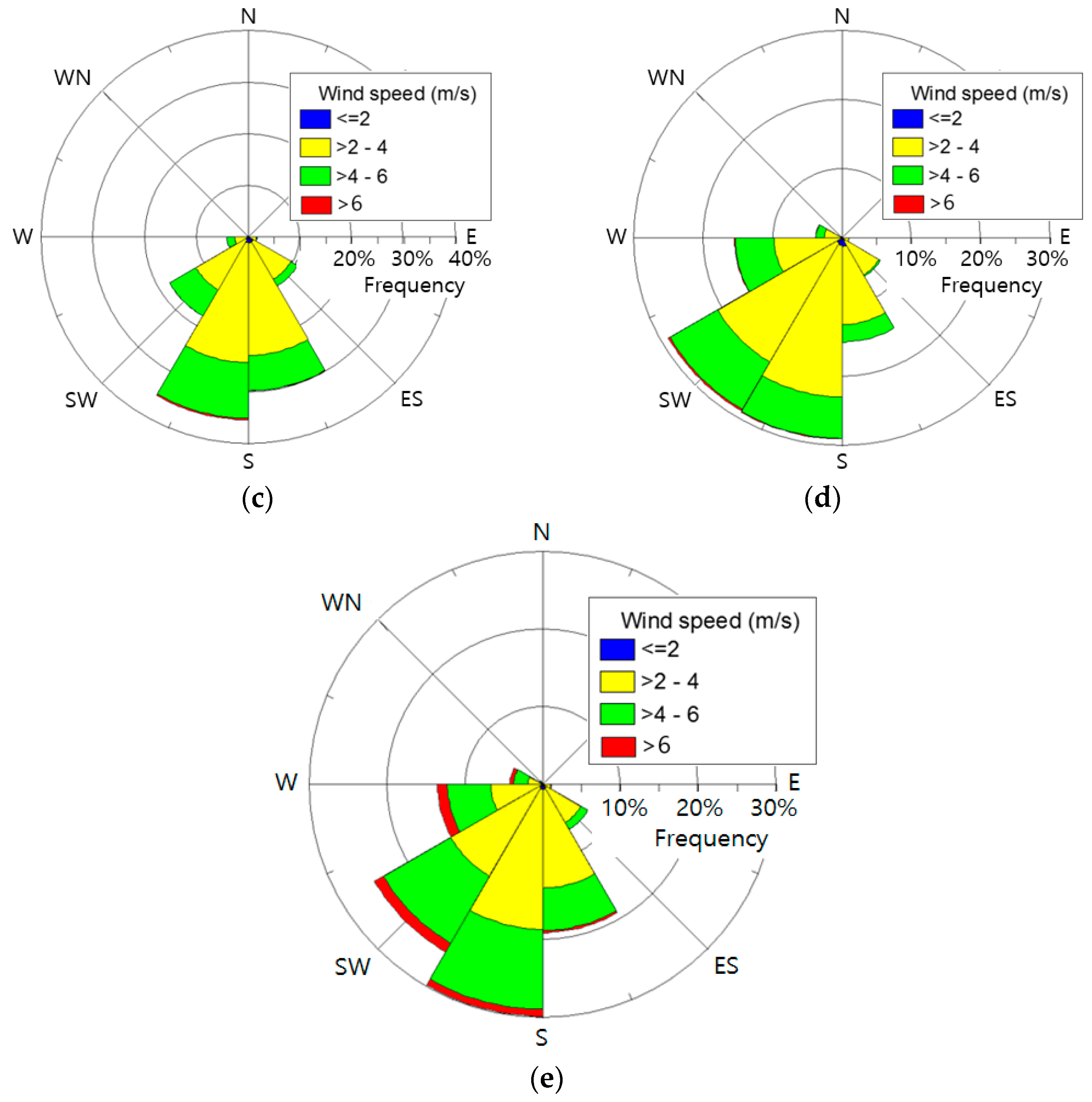
Figure 3 are the wind rose diagrams for all four seasons from 2005 to 2015 at Deokjeok-do. As shown in the figure, spring has a relatively higher wind speed than the other seasons while the main wind direction is southwest. It is clear that the prevailing wind directions are either south or southwest for all years. The determination of the prevailing wind direction is very important in order to maximize the energy production from wind turbine.
Figure 4 shows the frequency distribution of wind speeds at Deokjeok-do, estimated using Weibull parameters, for all four seasons from 2005 to 2015. Weibull plots are used for assessing the wind energy potential of the site, and it provides the percentage of the total wind speed, which is between cut-in and cut-out wind speeds of a wind turbine. In the figure, it is observed that most of the wind speeds are in the range of 3.5–4.5 m/s during all seasons. Relatively higher magnitudes of mean wind speed are observed during the spring as compared to all other seasons, which corresponds to the results of the wind roses in Figure 3. From cumulative distribution curves, it is clear that 95 percent of the total winds are below 6 m/s for all seasons.
Table 3 and Table 4 represent all of the important statistical parameters indicating the wind potential at Baengnyeong-do and Seo-San, respectively.
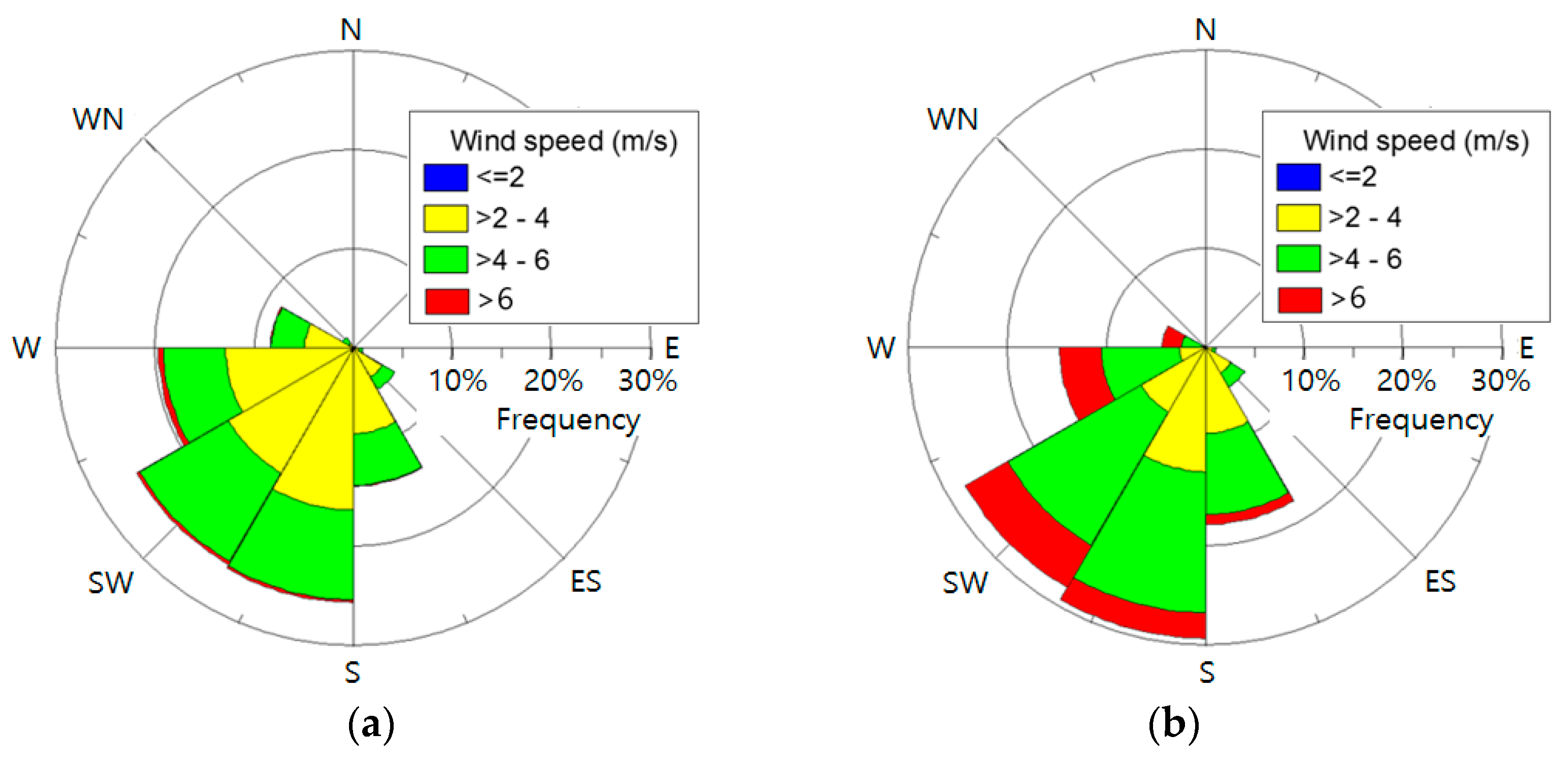
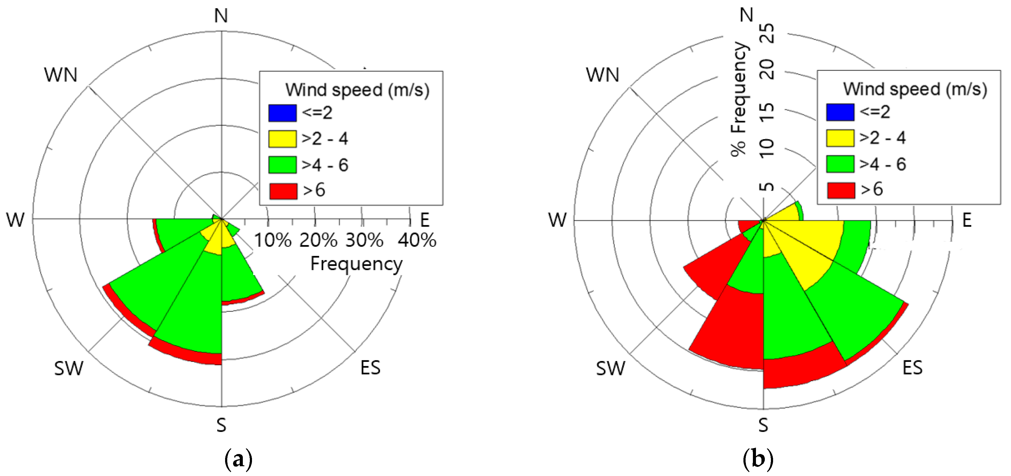
Annual mean wind speeds at Seo-San have the highest magnitude, as compared to the other two locations, Deokjeok-do and Baengnyeong-do, while the standard deviation (SD) is also relatively high. Wind data at Seo-San is consistent over the long period, which is beneficial for wind power generation. It is noted that the standard deviation (SD) at Baengnyeong-do is the lowest among three locations. Figure 5 shows the wind rose diagrams at Baengnyeong-do and Seo-San. The wind rose of Baengnyeong-do is drawn using wind data measured between 2005 and 2015, while the wind rose of Seo-San is obtained by using the wind data between 1997 and 2016. As shown in the figure, the prevailing wind directions are southwest and southeast for Baengnyeong-do and Seo-San, respectively. Seo-San has relatively stronger winds as compared to other two locations because the percentage of wind speeds greater than 6 m/s is the highest.
Figure 6 shows the Weibull distribution with respect to wind speed at Baengnyeong-do and Seo-San. Each measuring period is the same, as shown in Figure 5. As shown in the figure, the wind speed at Baengnyeong-do has a more concentrated distribution than those at Seo-San, around the mean speed of 5 m/s. From the cumulative distribution curves, it is clear that 50 percent of the total winds are above 5 m/s at Seo-San, as compared to Baengnyeong-do, which is having a value around 35 percent. Similarly, Seo-San has 10 percent of winds above 7 m/s. whereas Baengnyeong-do has no winds above 7 m/s, indicating that Seo-San has a relatively higher energy potential.
2.3. Wind Turbine Selection
2.3.1. Wind Turbine Class
To maximize the energy production and economic benefits, it is important to determine the optimal type of wind turbine for each site. The wind turbine class is a key parameter when designing the complex process of the wind power system. Wind turbine classes are categorized by annual mean wind speed, 50-year (1-year) extreme gust return speed, and the turbulence intensity in the wind at the installation site. It is important to mention that all these parameters must be estimated at the turbine hub height. There are four classes of wind turbines as defined by the international electro-technical commission (IEC, IEC code 61400-1), as shown in Table 5. Wind turbine class I corresponds to large wind turbines (high wind speeds at turbine hub height) and vice versa for class IV(S).
2.3.2. Extreme Wind Speed (EWS) and Turbulence Intensity (TI)
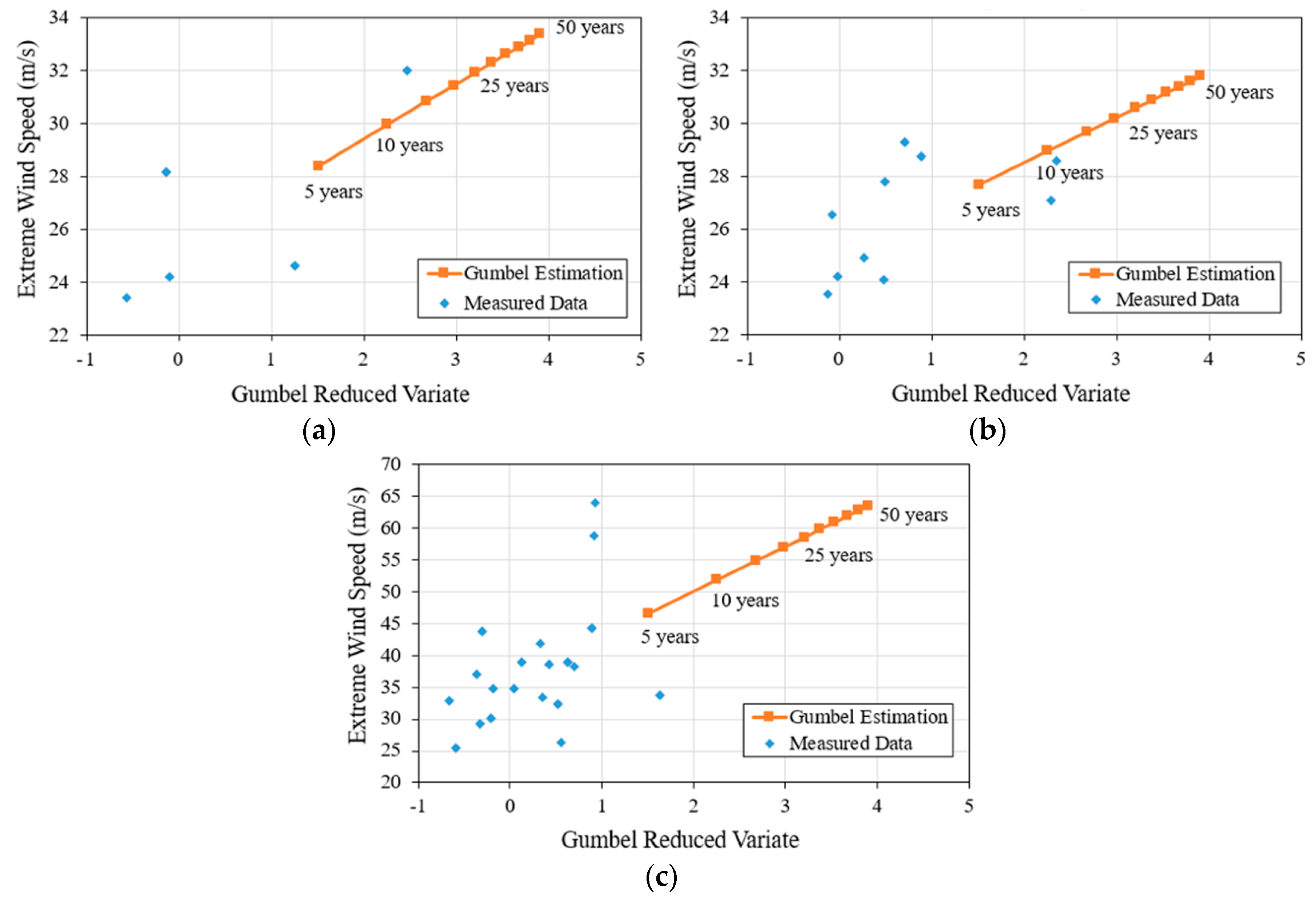
As described above, the wind turbine classes are categorized according to the 50-year (1-year) gust return speed. Estimation of EWS has a key role to play while selecting an optimal wind turbine. The generalized extreme value (GEV) distribution as explained by Von Mises (1936), is commonly used to estimate the EWS. It can be estimated by using Equation (12), with “t” as the return period in years [21]:
where β is the mode of the extreme value distribution (also known as the location parameter), and is the dispersion (or scale parameter, Gumbel parameters). Actually, β and are the y-intercept and the slope of Gumbel distribution graph, respectively.
Figure 7 is the plot of the following equations, in which the variable x is the maximum value of wind speed i.e., the EWS, selected from the time series of observations for each time period and the variable y is the Gumbel reduced variate (GRV). Equation (13) is the simplified version of Equation (12) as inserting Equations (14) and (15) into Equation (13) will result exactly in Equation (12):
where F(x) is the probability that the annual maximum wind speed is less than x. F(x) can be estimated for each of the observed annual maxima, by simply ordering the data from the smallest (x1) to the largest (xN), and calculating an empirical value of F(xm) from the ranked position of xm. For every value of x there is one value of F(x), hence for each value of x there is one value of GRV as well.
Figure 7 shows the estimation of EWS at the three locations. It should be noted that the typical hub height of the wind turbine is assumed to be 90 m in current case. The second parameter which should be taken into consideration while selecting a wind turbine for a particular site is TI. TI determines the sub-class of wind turbine (A to C) and the variation of TI with wind speed for each sub-class, as prescribed by IEC standard, is shown in Figure 8.
TI is defined as the ratio of standard deviation to mean wind speed [22]. The estimation of TI is very important, as it effects the structural integrity, as well as the aerodynamic performance of the wind turbine. As shown in Figure 8, the measured TI at 90 m height (assumed as hub height at this point) is extremely low, so wind turbines of any sub-class (A, B or C) are a safe choice for all three locations.
2.4. Selected Wind Turbines for Each Site
After analyzing the wind data (especially mean wind speed), the EWS and the TI, five wind turbines for each site were shortlisted as potential candidates to be selected for installation.
Figure 9 shows the power curves of wind turbines selected in the present study. These power curves are obtained at an air density of 1.225 kg/m3. Five of the same wind turbines were selected for Deokjeok-do and Baengnyeong-do, whereas wind turbines for Seo-San were selected separately because of its higher wind potential.
Table 6 and Table 7 represent the specifications of the selected wind turbines. It is to be noted that the hub heights of the wind turbines are not fixed here, because later on a sensitivity analysis will be performed in order to analyze the effect of turbine hub height on its economics. All selected wind turbines are manufactured in South Korea, hence reducing the transportation costs, as well as simplifying the economic calculations. Rotor diameter (m) and rated power (kW) of each wind turbine model is also apparent from its name, for instance; wind turbine model STX 93/2000 has rotor diameter of 93 m and rated power is 2000 kW.
2.5. Methodology for Technical and Economic Analysis
After selecting the wind turbines, the next step is to evaluate the performance of each wind turbine by estimating its power production and annual energy production (AEP). The general expression for estimating the wind turbine’s average power output is as follows:
where f(v) is the Weibull PDF curve of the test site, and Pt(v) is the power curve of selected wind turbine. The following expression is used in the present study to estimate the average power output of each wind turbine [23]:
where NB is number of wind speed bins. AEP and CF can be estimated using the following two equations, respectively:
where “t” is particular period of time for which the wind turbine’s average energy output will be estimated, and PR is the rated power of the wind turbine. While estimating the AEP of each wind turbine, transformer losses were considered as 1%, grid losses as 3%, wake losses as 6%, and turbine availability as 95% [3].
Along with technical feasibility, the economic feasibility of a wind power project must also be analyzed in advance. All the shortlisted wind turbines must go through an economic evaluation as well. Generally used economic parameters are NPV, IRR, LCOE and PBP. All of these parameters will be discussed and estimated for all of the selected candidate wind turbines. The cost of the wind turbine, CwT (k€) can be estimated using Equation (20) [24]:
where is the rated power of wind machine in MW. NPV is defined as follows:
where n is the project’s lifetime (20 years), t is the time period (years), r is the discount rate, Bt are all the benefits during a particular year t, for instance incomes from selling electricity, depreciation credits, production tax credits (PTC) and investment tax credits (ITC). Similarly, Ct are costs, which are basically of two types, initial investment and annually occurring costs. Initial investment includes turbine’s price (blades and nacelle with gear box and generator, as estimated from Equation (20)), tower price, transportation, and installation cost. The last two costs are assumed as 30% of the wind turbine’s price [5]. All other types of initial investments like cables cost, grid connection, etc. are ignored for the sake of simplifying the calculations. On the other hand, annually recurring costs considered in this study include; tax on income and the annual O&M cost, whereas the later one is assumed as 5% of the wind turbine’s price [5]. A project with a relatively higher value (must be greater than zero) of NPV is the most economically feasible project. Another important parameter is internal rate of return (IRR), which is the value of the discount rate at which project’s NPV becomes zero, i.e., the present worth of all costs becomes equal to the present worth of all benefits. Setting Equation (21) equal to zero results in Equation (22), in which the discount rate is IRR:
A project is considered as financially feasible if the IRR is greater than the financial discount rate and also, the IRR is the maximum discount rate, up to which the project can be economically feasible. The levelized cost of electricity (LCOE, €/kWh), is the present value of the cost to produce one unit of electrical energy, considering the lifetime of the project. LCOE can be estimated using the following equation [5] (all the variable in the definition of LCOE are defined in the Nomenclature section):
Finally, the simple payback period (PBP) is the time in which the initial cash outflows of an investment are expected to be recovered from the cash inflows in the following years. It is one of the simplest investment appraisal techniques and calculated using Equation (24):
3. Results and Discussion
3.1. Analysis of Wind Turbines for Deokjeok-Do
One of the most important parameters which affects the economics of wind farms is the turbine hub height. Along with hub height, other factors which highly affect the economics of wind farms are (but not limited to), electric tariff (€/MWh), discount rate (%) and corporate tax rate (%). However, accurate prediction of these three parameters is not a straightforward process and it is beyond the scope of current study. Hence for the sake of calculations and estimating NPV & LCOE, these three values were assumed and are presented in Table 8.
As it is obvious that increasing the hub height will generate more electricity, but the factors like economy, structural issues and cut-off wind speeds of the wind turbine put constraints on the turbine hub height. Therefore, it is important to optimize the hub height in order to maximize the profits. But the questions arise as what should be the minimum and maximum hub heights (Hmin and Hmax). Hmin is constrained by the “minimum ground clearance” whereas Hmax should be bounded by the technology available to install and operate turbines on tall towers. The ground clearance of a commercial turbine is the height of the blade tip at its lowest position (when the blade is vertically down). The minimum practical value was taken as 75 ft. (22.86 m), e.g., Ref. [26].
On the other hand, taller towers are employed to avoid the large wind shear and high turbulence levels at relatively low heights, caused partly by the topography [27]. Engstrom et al. [27] described welded steel shell towers for large turbines, and concluded that the available technology can provide towers up to 150 m for 3 MW turbines. Moreover, many operating turbines were installed with hub heights > 140 m. To this end, the lower and upper limits for hub heights in the analysis were taken as 80 m and 140 m, respectively.
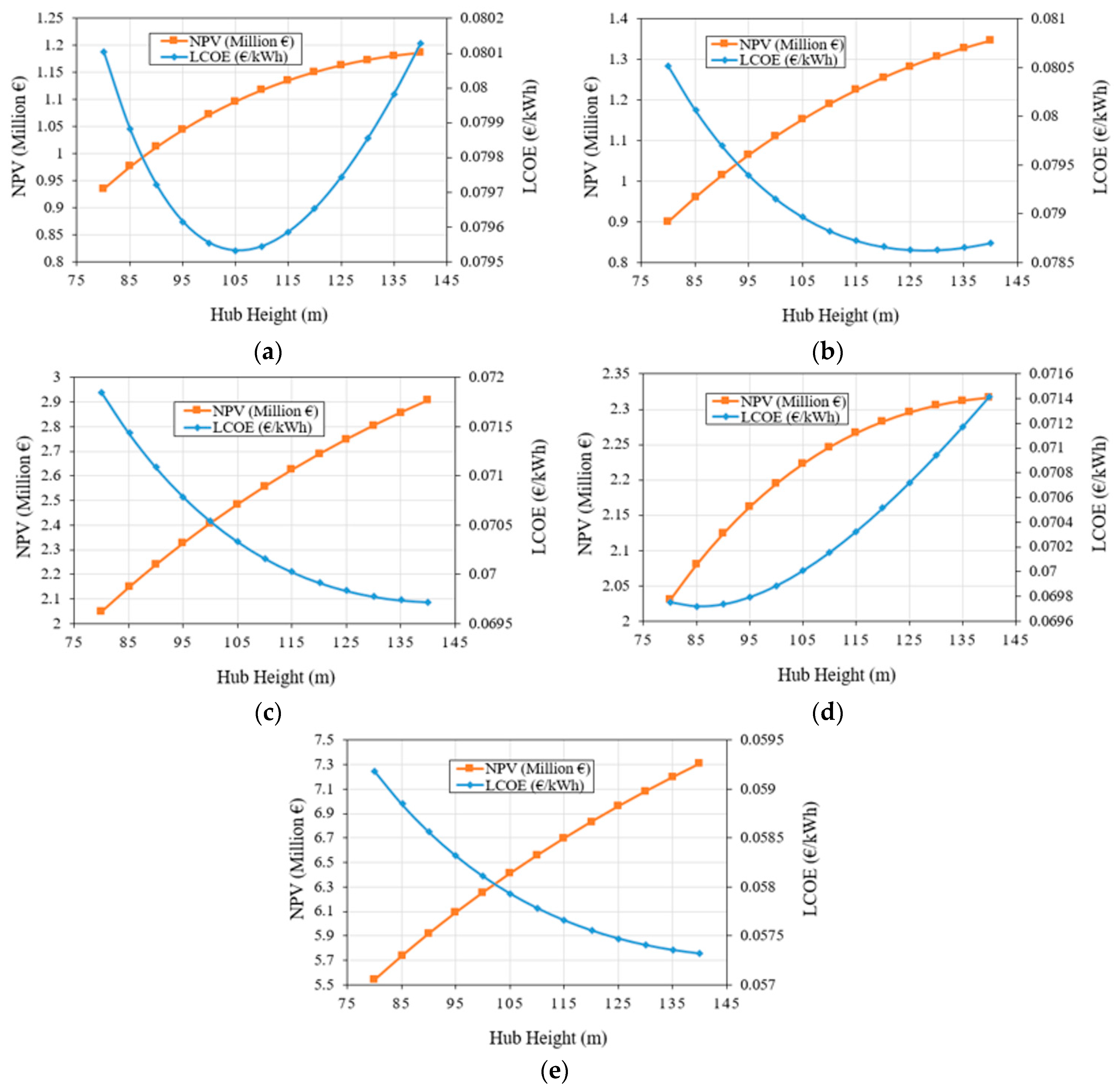
Figure 10 shows the variation in NPV and LCOE by changing the turbine hub height. It is clear from Figure 10 that NPV is negative for all the wind turbines considered for Deokjeok-do except the wind turbine model WinDS 134/3000. The main reason behind this behavior is the cost of the tower, which dominates over the benefits obtained from selling extra units of electricity generated, due to increase in turbine hub height.
The optimum hub height is defined as hub height at which both LCOE is at a minimum and NPV is at a maximum, or just LCOE is at the minimum. According to these criteria, the optimum hub height for WinDS 134/300 is 140 m as shown in Table 10. It is to be noted other parameters were not calculated for remaining wind turbines, as if NPV is negative, there is no value of looking into that project.
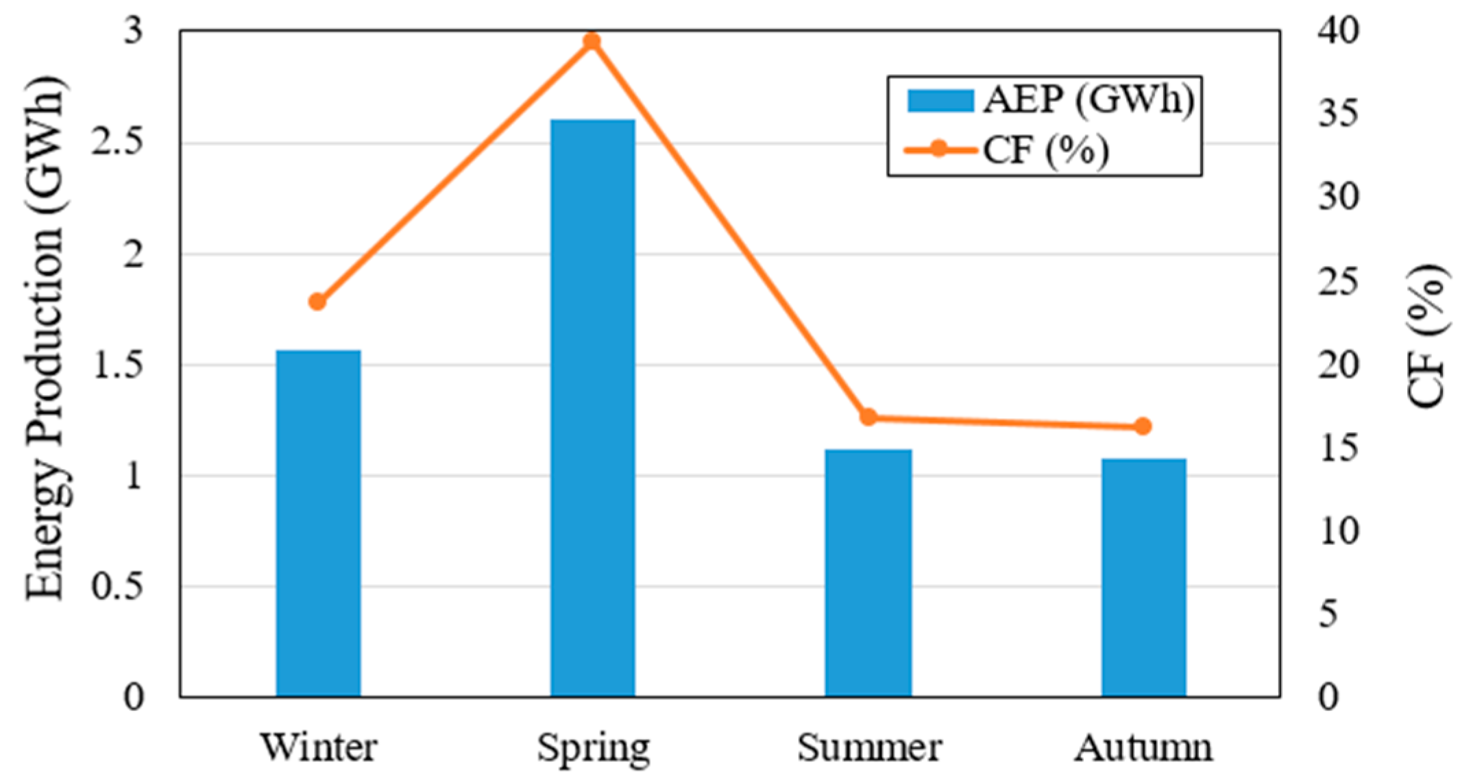
Figure 11 shows the energy production based on season at Deokjeok-do using the model WinDS 134/3000 wind turbine having the installation height of 140 m. As it was shown in Figure 3b and Figure 4b that spring is the “windiest” season, so the energy production during spring is at its maximum at Deokjeok-do.
3.2. Analysis of Wind Turbines for Baengnyeong-Do
Figure 12 shows the hub height sensitivity analysis results of all wind turbines considered for Baengnyeong-do. Although all the wind turbines have positive values of NPV at all hub heights considered, the WinDS 134/3000 (Doosan, Korea) is an optimized wind turbine model with a hub height of 140 m, as this combination will generate net profits having NPV of 7.32 million euros (the maximum) and LCOE will be as low as 0.0573 €/kWh (the minimum).
After determining the optimum hub height for each wind turbine, all important technical and financial parameters were estimated, and are presented in Figure 13. It is very important to note that AEP estimations have been made using optimal hub heights of each wind turbine and optimal hub heights of WinDS134/3000, which is the optimum wind turbine in the current scenario as well, is the 140 m hub height.
Apart from results presented in Figure 13, one other parameter which can also effect the selection of wind turbine is the initial investment. As it is clear that choosing wind turbine model WinDS 134/3000, will not only require the highest initial capital, but also the annual O&M cost would be the highest. So, from the practical point of view, it really depends upon how much capital is available to build the wind farm at Baengnyeong-do. But according to our analysis installation of a WinDS 134/3000 turbine is recommended because the payback period of the initial investment will be a minimum of 6.2 years. Figure 13e shows the breakdown of AEP of WinDS 134/3000, at the hub height of 140 m, into seasons.
3.3. Analysis of Wind Turbines for Seo-San
Figure 14 shows the hub height sensitivity analysis results of all wind turbines considered for Seo-San. In Figure 14, it is noted that the wind turbine model HJWT 87/2000 is the best wind turbine in the present scenario. However, the variation of NPV and LCOE with the turbine hub height, for this wind turbine model is a little tricky. As the hub height increases both the parameters i.e., NPV and LCOE increase, so it was decided that the 110-m hub height will be considered as the optimum hub height for HJWT 90/2000.
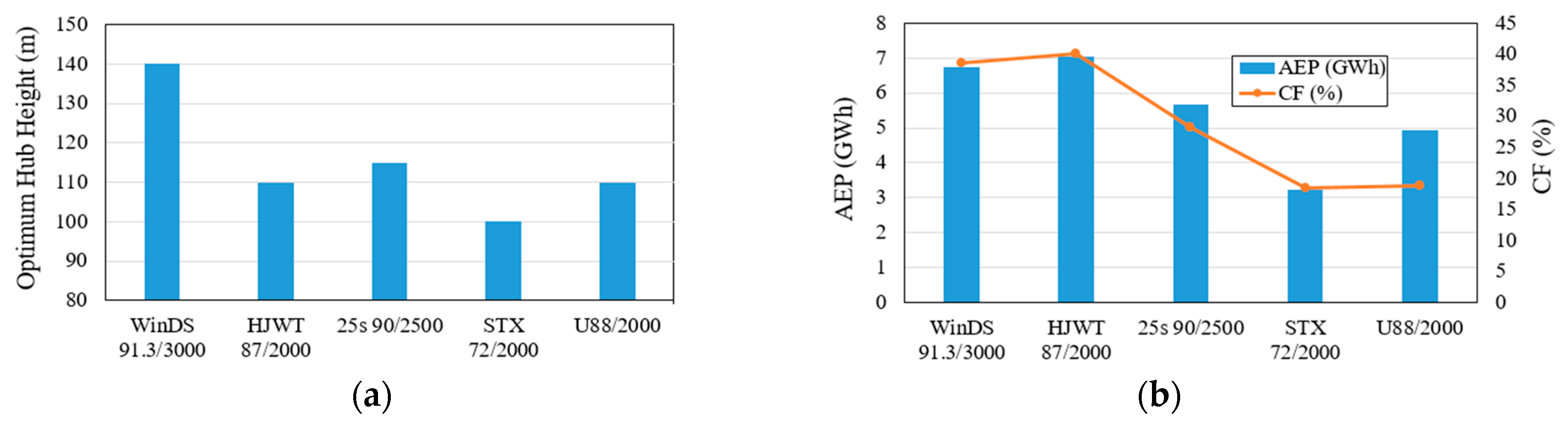
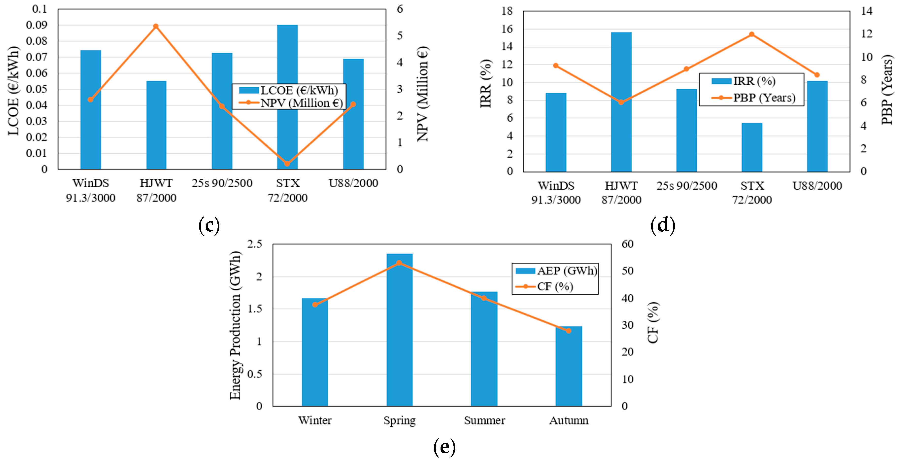
Figure 15 shows the comparisons of techno-economic performance for each wind turbine at the corresponding optimal hub height as determined from Figure 14. It is clear from Figure 15 that the HJWT 87/2000 wind turbine model (Hanjin, Korea) has all types of competitive edges over its competitors, so it is recommended that the wind turbine model HJWT 87/2000 at hub height of 110 m should be installed at Seo-San, in case a wind farm is planned to be built at this site. Unlike the WinDS 134/3000 wind turbine model, which is recommended for Deokjeok-do and Baengnyeong-do, the HJWT 87/2000 will require a minimum capital investment as compared to other wind turbines. Figure 15e shows the same trend as observed in Figure 11 and Figure 13e, i.e., the maximum energy production is in spring, so it can be concluded that spring is the most suitable season for harnessing wind energy at all three locations.
4. Conclusions
The current paper analyses the wind energy potential and feasibility of installing wind power system at three locations in South Korea named as Deokjeok-do, Baengnyeong-do and Seo-San. A detailed technical and economic analysis have been conducted in order to select the most suitable wind turbines for all three regions. First of all, the wind data analysis was conducted and it was found that the overall mean wind speed at Deokjeok-do during 2005–2015 was 3.8 m/s, at Baengnyeong-do during 2001–2016 was 4.6 m/s and at Seo-San during 1997–2016 was 5 m/s. In order to shortlist the most suitable wind turbines, 50-years extreme gust returns were estimated at all three locations, using the graphical method of Gumbel distribution and they are approximately 33 m/s, 24 m/s and 56 m/s for Deokjeok-do, Baengnyeong-do and Seo-San, respectively. The turbulence intensity (TI) in wind speeds at all three locations is found to be significantly less than turbulence intensity curves provided by IEC. So according to EWS, TI and some other wind characteristics, the wind turbine classes best suited for Deokjeok-do and Baengnyeong-do are IEC III or IEC class IV (class S), whereas Seo-San has relatively stronger winds and the wind turbines best suited for this region belongs to either IEC class I or II.
The WinDS 134/3000 wind turbine model is technically and economically the most feasible wind turbine for Deokjeok-do and Baengnyeong-do according the current scenario. It can produce 6.37 MWh of electricity per year at Deokjeok-do, whereas its AEP is almost 10 MWh for Baengnyeong-do. Similarly the HJWT 87/2000 wind turbine model can produce ~7 MWh of electricity per year and also other financial parameters like NPV, PBP, IRR and LCOE suggest that it is recommended to be installed at Seo-San. Wind turbine hub height affects the economics of the wind turbine, so the optimal hub height was estimated for each wind turbine model. The Optimum hub heights for “WinDS 134/3000” at Deokjeok-do and Baengnyeong-do is 140m and for Seo-San, the optimal hub height of “HJWT 87/2000” is 110 m.
Acknowledgment
This work was supported by the new and renewable energy core technology program of the Korean Institute of Energy Technology Evaluation and Planning (KETEP), granted financial resources from the Ministry of Trade, Industry and Energy, Republic of Korea (No. 20153010130310).
Author Contributions
Sang-Moon Lee and Choon-Man Jang requested KMA and collected the wind data. Sajid Ali analyzed the data and wrote the paper.
Conflicts of Interest
The authors declare no conflict of interest.
Nomenclature
| f(v) | Weibull PDF |
| F(v) | Weibull CDF |
| k | Weibull shape parameter |
| c | Weibull scale parameter |
| v | Wind speed |
| Bt | Benefits |
| Ct | Costs |
| r | Discount rate |
| It | Investment made in year t |
| Dt | Depreciation credit |
| Tt | Tax levy |
| vm | Mean wind speed |
| t | Time |
| n | Number of wind data |
| vi | Instantaneous wind speed |
| VR | Wind speed at reference height |
| ygumbel | Gumbel reduced variate |
| F(x) | Probability of annual max. speed |
| Pt(v) | Wind turbine power at wind speed v |
| Pave | Average wind turbine power |
| NB | Number of speed bins |
| PR | Rated power of wind turbine |
Greek Letters
| Σ | Summation |
| Г | Gamma Function |
| β | Gumbel location parameter |
| α | Gumbel scale parameter |
Abbreviations
| probability density function | |
| CDF | cumulative distribution function |
| SD | Standard deviation |
| IEC | International electro-technical commission |
| EWS | Extreme wind speed |
| GRV | Gumbel reduced variate |
| TI | Turbulence intensity |
| AEP | Annual energy production |
| CF | Capacity factor |
| NPV | Net present value |
| IRR | Internal rate of return |
| LCOE | levelized cost of electricity |
| O&M | Operating and maintenance cost |
| PBP | Payback period |
References
- Jang, J.K.; Yu, B.M.; Ryu, K.W.; Lee, J.S. Offshore wind resource assessment around Korean Peninsula by using QuikSCAT satellite data. J. Korean Soc. Aeronaut. Space Sci. 2009, 37, 1121–1130. [Google Scholar] [CrossRef]
- Oh, K.Y.; Kim, J.Y.; Lee, J.K.; Ryu, M.S.; Lee, J.S. An assessment of wind energy potential at the demonstration offshore wind farm in Korea. Energy 2012, 46, 555–563. [Google Scholar] [CrossRef]
- Kim, H.; Kim, B. Wind resource assessment and comparative economic analysis using AMOS data on a 30 MW wind farm at Yulchon district in Korea. Renew. Energy 2016, 85, 96–103. [Google Scholar] [CrossRef]
- Lee, M.E.; Kim, G.; Jeong, S.T.; Ko, D.H.; Kang, K.S. Assessment of offshore wind energy at Younggwang in Korea. Renew. Sustain. Energy Rev. 2013, 21, 131–141. [Google Scholar] [CrossRef]
- Kim, J.Y.; Oh, K.Y.; Kang, K.S.; Lee, J.S. Site selection of offshore wind farms around the Korean Peninsula through economic evaluation. Renew. Energy 2013, 54, 189–195. [Google Scholar] [CrossRef]
- Oh, K.Y.; Kim, J.Y.; Lee, J.S.; Ryu, K.W. Wind resource assessment around Korean Peninsula for feasibility study on 100 MW class offshore wind farm. Renew. Energy 2012, 42, 217–226. [Google Scholar] [CrossRef]
- Sanseverino, E.R.; Sanseverino, R.R.; Favuzza, S.; Vaccaro, V. Near zero energy islands in the Mediterranean: Supporting policies and local obstacles. Energy Policy 2014, 66, 592–602. [Google Scholar] [CrossRef]
- Cosentino, V.; Favuzza, S.; Graditi, G.; Ippolito, M.G.; Massaro, F.; Sanseverino, E.R.; Zizzo, G. Smart renewable generation for an islanded system. Technical and economic issues of future scenarios. Energy 2012, 39, 196–204. [Google Scholar] [CrossRef]
- Lee, M.J. South Korea Blackout Risk Rises. Wall Str. J. 2013, 17, 2–14. [Google Scholar]
- Available online: https://data.kma.go.kr/ (accessed on 18 September 2017).
- Akdağ, S.A.; Dinler, A. A new method to estimate Weibull parameters for wind energy applications. Energy Conver. Manag. 2009, 50, 1761–1766. [Google Scholar] [CrossRef]
- Akgül, F.G.; Şenoğlu, B.; Arslan, T. An alternative distribution to Weibull for modeling the wind speed data: Inverse Weibull distribution. Energy Conver. Manag. 2016, 114, 234–240. [Google Scholar] [CrossRef]
- Carneiro, T.C.; Melo, S.P.; Carvalho, P.C.; Braga, A.P.D.S. Particle Swarm Optimization method for estimation of Weibull parameters: A case study for the Brazilian northeast region. Renew. Energy 2016, 86, 751–759. [Google Scholar] [CrossRef]
- Hennessey, J.P., Jr. Some aspects of wind power statistics. J. Appl. Meteorol. 1977, 16, 119–128. [Google Scholar] [CrossRef]
- Corotis, R.B.; Sigl, A.B.; Klein, J. Probability models of wind velocity magnitude and persistence. Sol. Energy 1978, 20, 483–493. [Google Scholar] [CrossRef]
- Justus, C.G.; Hargraves, W.R.; Mikhail, A.; Graber, D. Methods for estimating wind speed frequency distributions. J. Appl. Meteorol. 1978, 17, 350–353. [Google Scholar] [CrossRef]
- Deaves, D.M.; Lines, I.G. On the fitting of low mean wind speed data to the Weibull distribution. J. Wind Eng. Ind. Aerodyn. 1997, 66, 169–178. [Google Scholar] [CrossRef]
- Garcia, A.; Torres, J.L.; Prieto, E.; de Francisco, A. Fitting wind speed distributions: A case study. Sol. Energy 1998, 62, 139–144. [Google Scholar] [CrossRef]
- Carta, J.A.; Ramirez, P.; Velazquez, S. A review of wind speed probability distributions used in wind energy analysis: Case studies in the Canary Islands. Renew. Sustain. Energy Rev. 2009, 13, 933–955. [Google Scholar] [CrossRef]
- Shu, Z.; Li, Q.; Chan, P. Statistical analysis of wind characteristics and wind energy potential in Hong Kong. Energy Conver. Manag. 2015, 101, 644–657. [Google Scholar] [CrossRef]
- Palutikof, J.; Brabson, B.; Lister, D.; Adcock, S. A review of methods to calculate extreme wind speeds. Meteorol. Appl. 1999, 6, 119–132. [Google Scholar] [CrossRef]
- IEC 61400-3: Wind Turbines—Part 1: Design Requirements; International Electro-Technical Commission: Geneva, Switzerland, 2005.
- Mirhosseini, M.; Sharifi, F.; Sedaghat, A. Assessing the wind energy potential locations in province of Semnan in Iran. Renew. Sustain. Energy Rev. 2011, 15, 449–459. [Google Scholar] [CrossRef]
- Dicorato, M.; Forte, G.; Pisani, M.; Trovato, M. Guidelines for assessment of investment cost for offshore wind generation. Renew. Energy 2011, 36, 2043–2051. [Google Scholar] [CrossRef]
- Min, C.G.; Park, J.K.; Hur, D.; Kim, M.K. The Economic Viability of Renewable Portfolio Standard Support for Offshore Wind Farm Projects in Korea. Energies 2015, 8, 9731–9750. [Google Scholar] [CrossRef]
- Oteri, F. An Overview of Existing Wind Energy Ordinances; National Renewable Energy Laboratory Technical Report; NREL/TP-500-44439; National Renewable Energy Laboratory: Golden, CO, USA, 2008.
- Engström, S.; Lyrner, T.; Hassanzadeh, M.; Stalin, T.; Johansson, J. Tall Towers for Large Wind Turbines; Report from Vindforsk Project; Elforsk AB: Stockholm, Sweden, 2010; p. 50. [Google Scholar]
Figure 1.
Locations of feasibility analysis (Source: Google Maps).
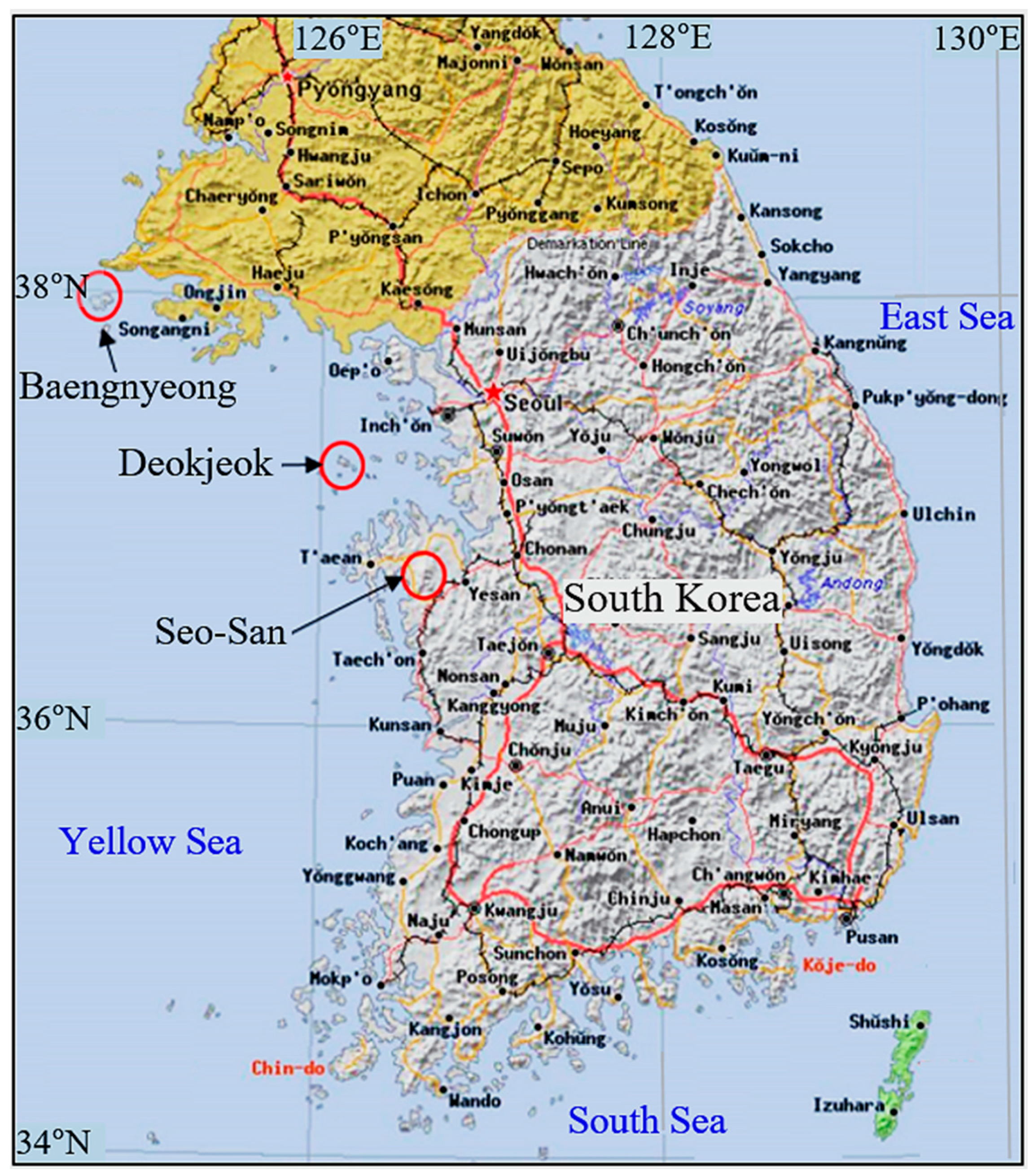
Figure 2.
Meteorological masts for wind data measurement (a) Deokjeok-do; (b) Baengnyeong-do; (c) Seo-San.
Figure 2.
Meteorological masts for wind data measurement (a) Deokjeok-do; (b) Baengnyeong-do; (c) Seo-San.
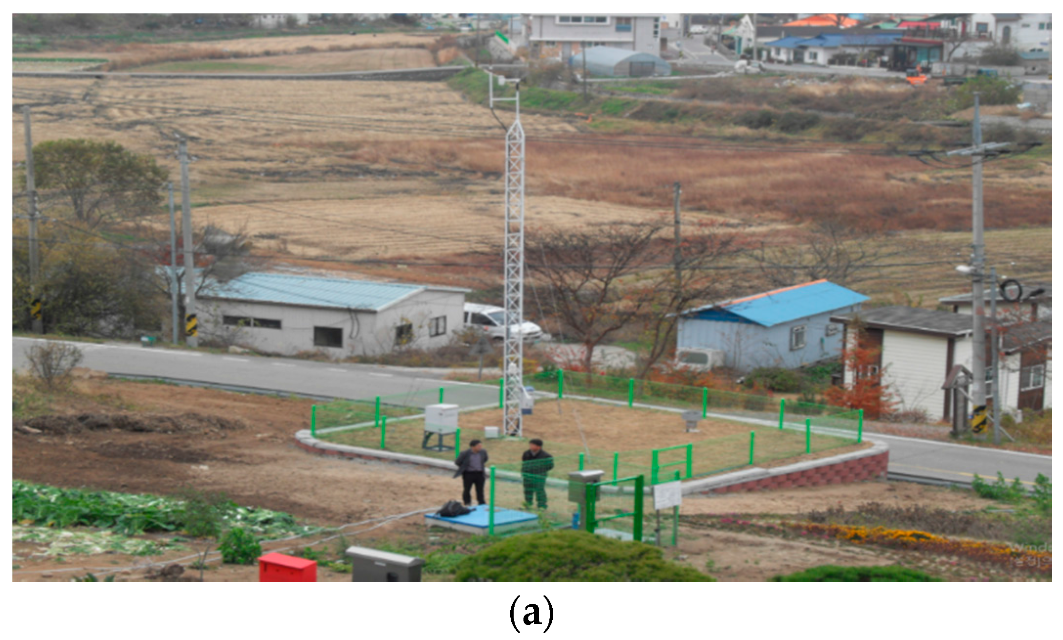
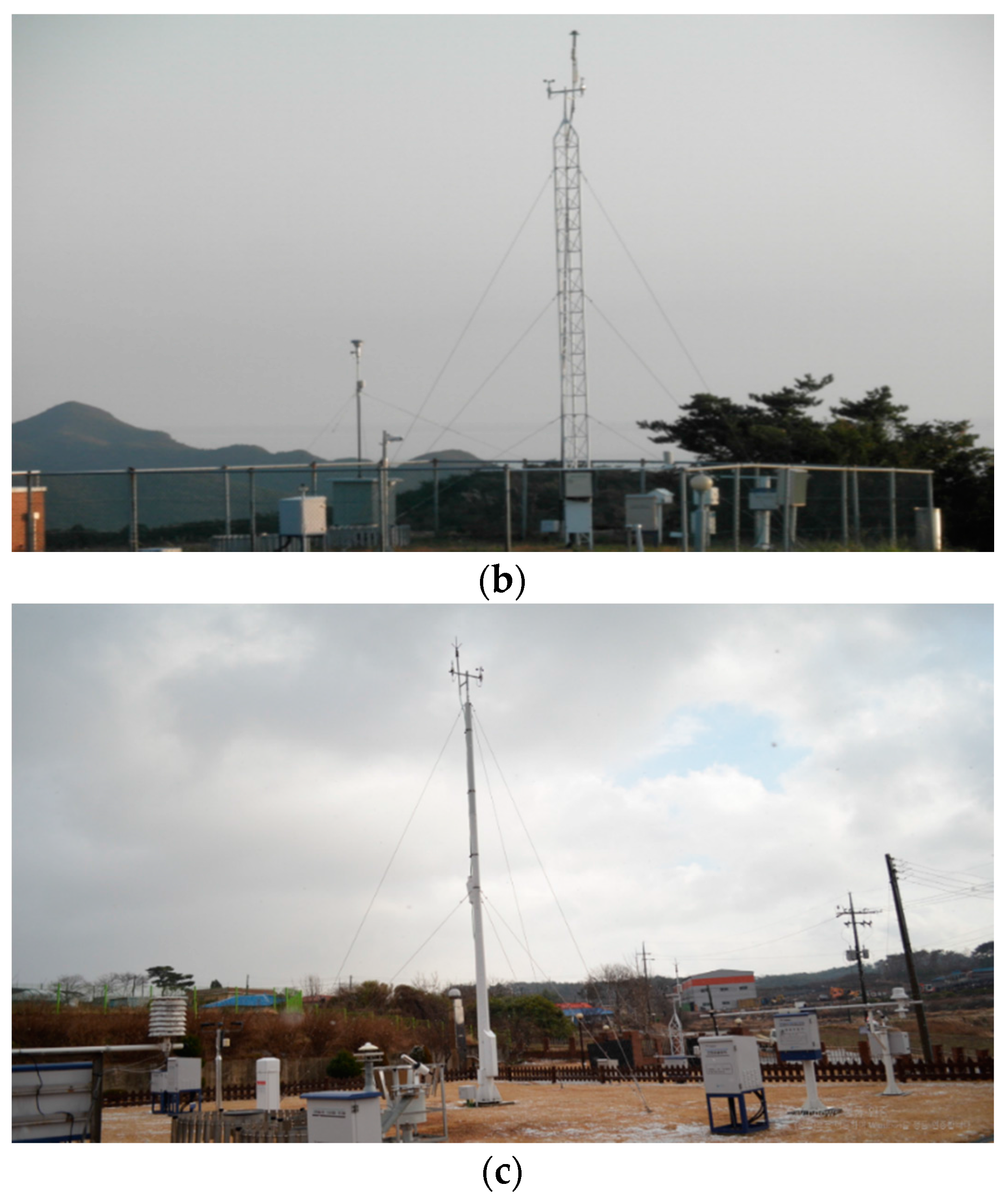
Figure 3.
Wind rose diagrams for Deokjeok-do from 2005 to 2015 at 10 m from local ground (a) Winter; (b) Spring; (c) Summer; (d) Autumn; (e) Overall.
Figure 3.
Wind rose diagrams for Deokjeok-do from 2005 to 2015 at 10 m from local ground (a) Winter; (b) Spring; (c) Summer; (d) Autumn; (e) Overall.


Figure 4.
Weibull distribution of Deokjeok-do from 2005 to 2015 at 10 m from the local ground (a) Winter; (b) Spring; (c) Summer; (d) Autumn; (e) Overall.
Figure 4.
Weibull distribution of Deokjeok-do from 2005 to 2015 at 10 m from the local ground (a) Winter; (b) Spring; (c) Summer; (d) Autumn; (e) Overall.
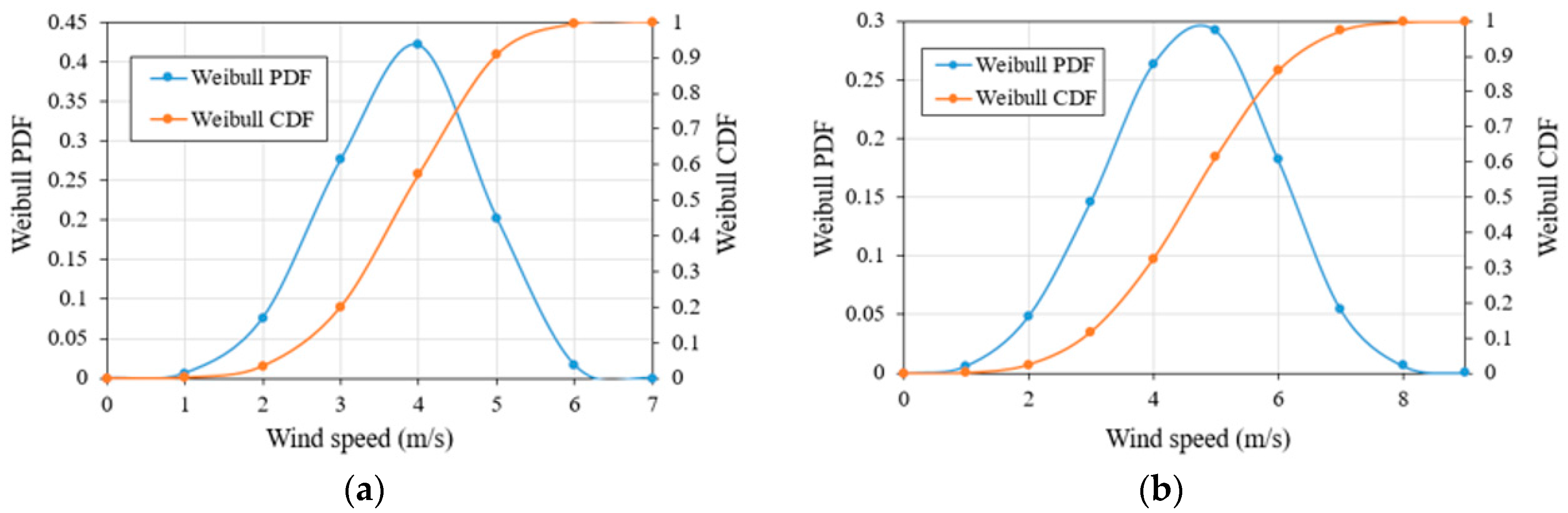
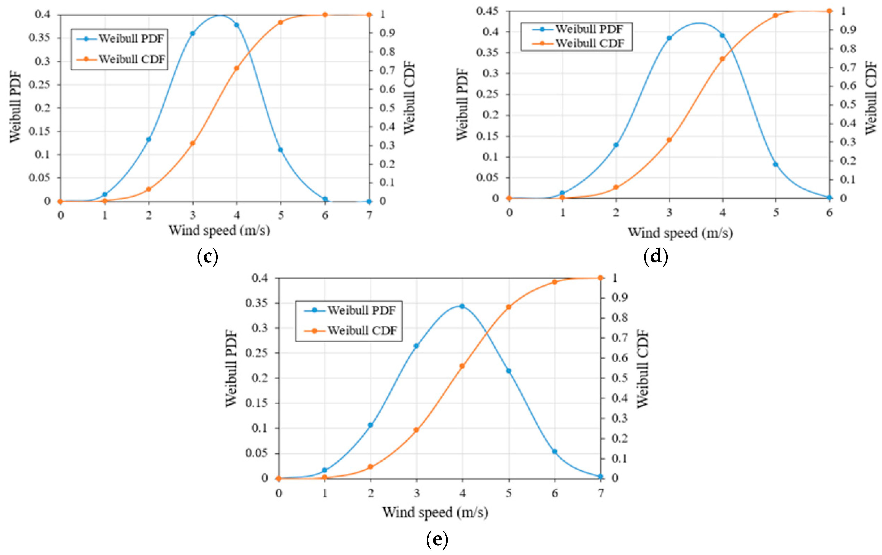
Figure 5.
Wind rose diagrams at 10 m from local ground (a) Baengnyeong-do from 2001 to 2016; (b) Seo-San from 1997 to 2016.
Figure 5.
Wind rose diagrams at 10 m from local ground (a) Baengnyeong-do from 2001 to 2016; (b) Seo-San from 1997 to 2016.

Figure 6.
Weibull distribution at 10 m from local ground (a) Baengnyeong-do from 2001 to 2016; (b) Seo-San from 1997 to 2016.
Figure 6.
Weibull distribution at 10 m from local ground (a) Baengnyeong-do from 2001 to 2016; (b) Seo-San from 1997 to 2016.
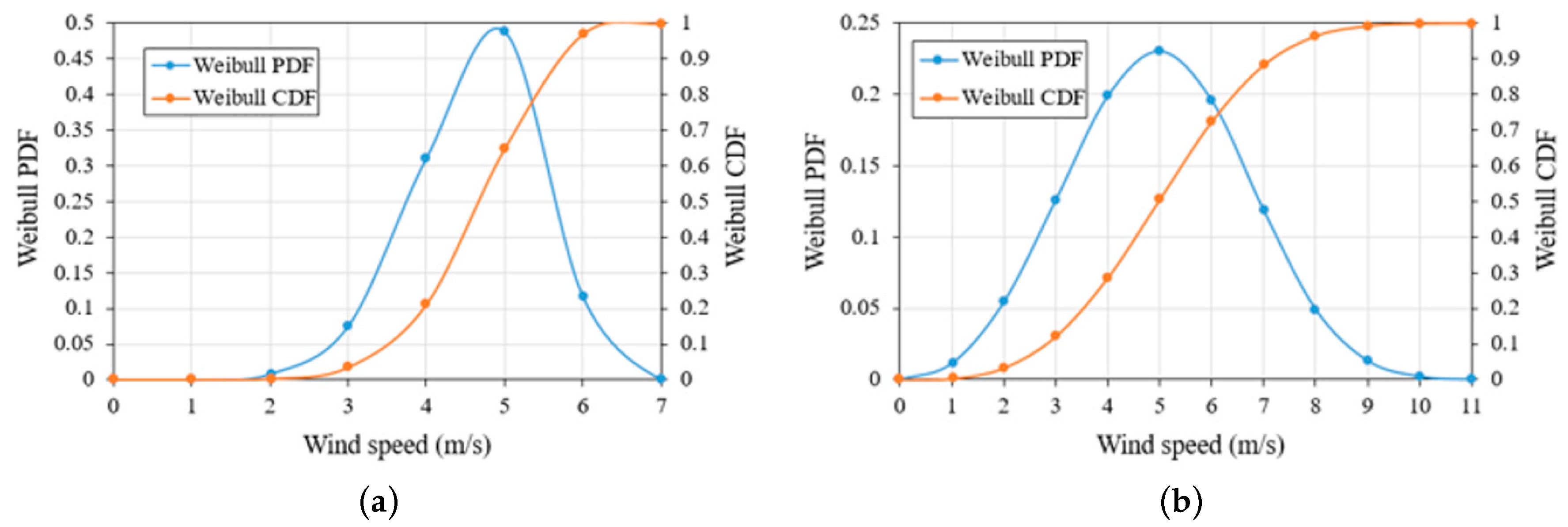
Figure 7.
Estimation of EWS (a) Deokjeok-do; (b) Baengnyeong-do; (c) Seo-San.

Figure 8.
Estimation of TI.
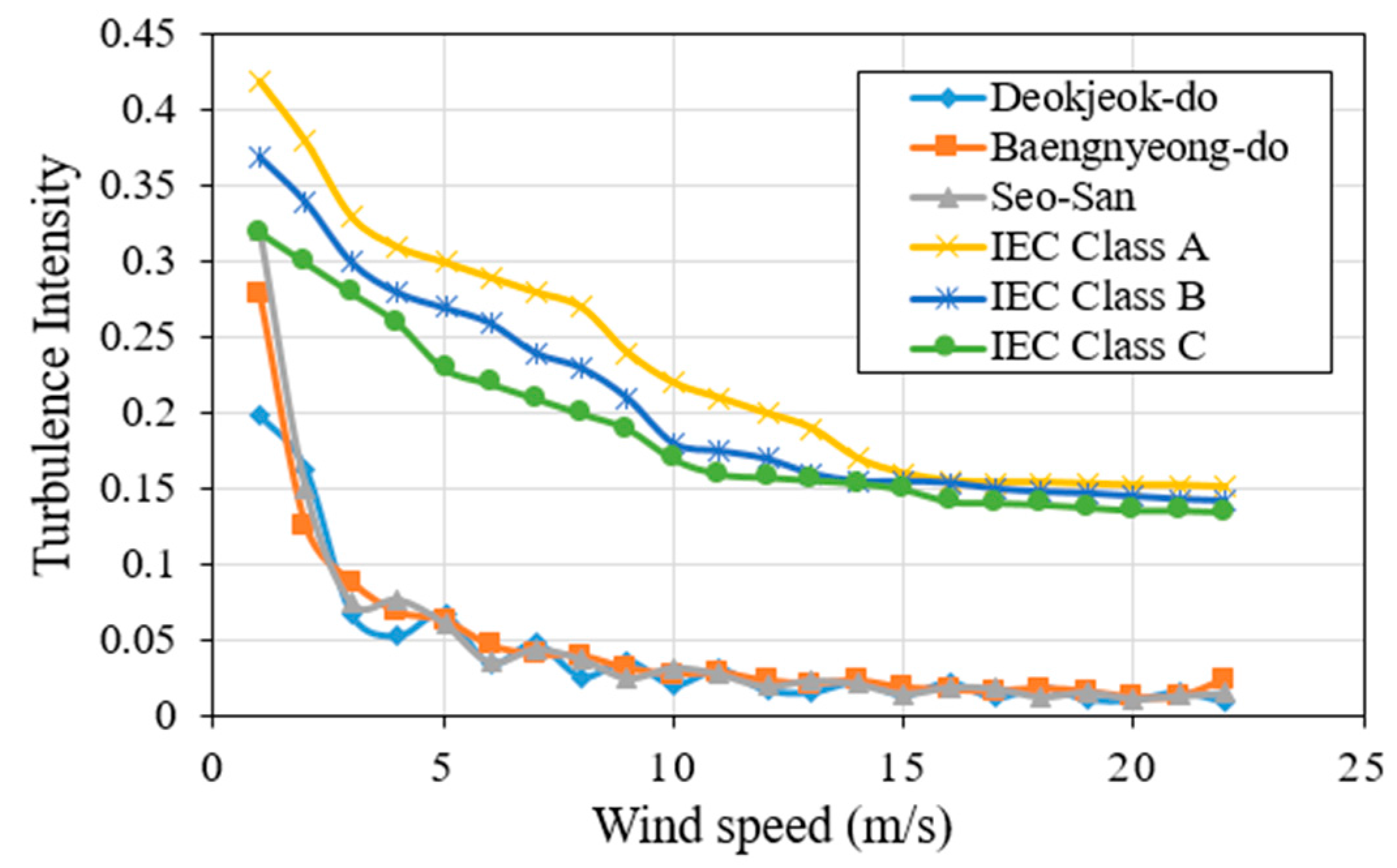
Figure 9.
Power curves of selected wind turbines (a) Deokjeok-do and Baengnyeong-do; (b) Seo-San.
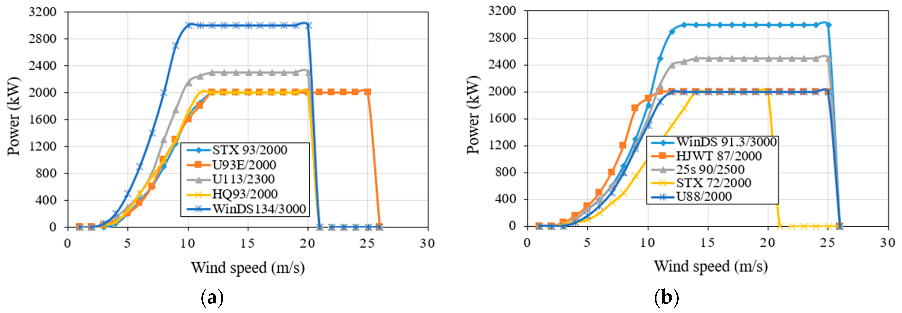
Figure 10.
Effect of hub height on wind turbines economics at discount rate of 5% for Deokjeok-do (a) STX 93/2000; (b) U 93E/2000;(c) U 113/2300; (d) HQ 93/2000; (e) WinDS 134/3000.
Figure 10.
Effect of hub height on wind turbines economics at discount rate of 5% for Deokjeok-do (a) STX 93/2000; (b) U 93E/2000;(c) U 113/2300; (d) HQ 93/2000; (e) WinDS 134/3000.
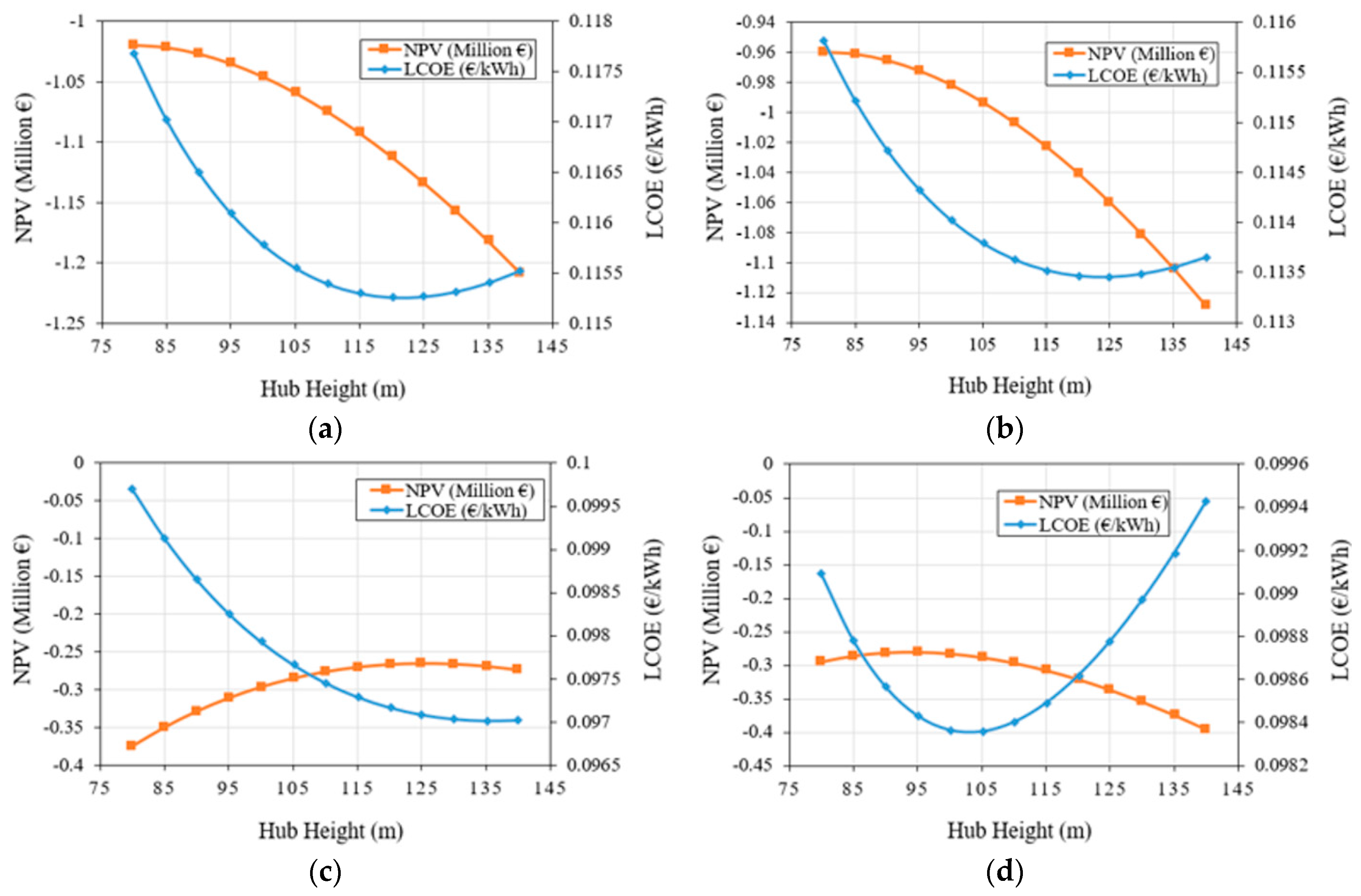
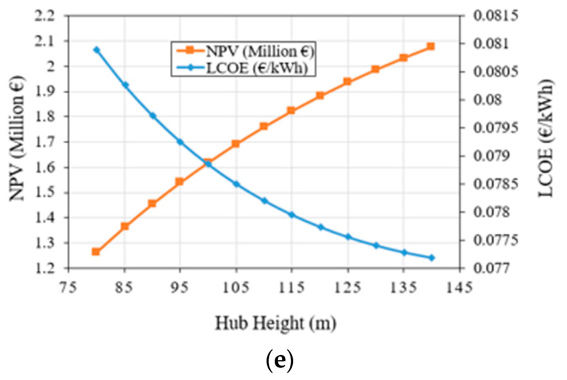
Figure 11.
Season-wise energy production of best suited wind turbine for Deokjeok-do at optimum hub height.
Figure 11.
Season-wise energy production of best suited wind turbine for Deokjeok-do at optimum hub height.

Figure 12.
Effect of hub height on wind turbines economics at discount rate of 5% for Baengnyeong-do (a) STX 93/2000; (b) U 93E/2000; (c) U 113/2300; (d) HQ 93/2000; (e) WinDS 134/3000.
Figure 12.
Effect of hub height on wind turbines economics at discount rate of 5% for Baengnyeong-do (a) STX 93/2000; (b) U 93E/2000; (c) U 113/2300; (d) HQ 93/2000; (e) WinDS 134/3000.

Figure 13.
Estimations of important parameters at discount rate of 5% and the optimal hub height for Baengnyeong-do (a) optimal hub height; (b) AEP & CF; (c) LCOE & NPV; (d) IRR & PBP; (e) Season-wise energy production of WinDS 134/3000.
Figure 13.
Estimations of important parameters at discount rate of 5% and the optimal hub height for Baengnyeong-do (a) optimal hub height; (b) AEP & CF; (c) LCOE & NPV; (d) IRR & PBP; (e) Season-wise energy production of WinDS 134/3000.
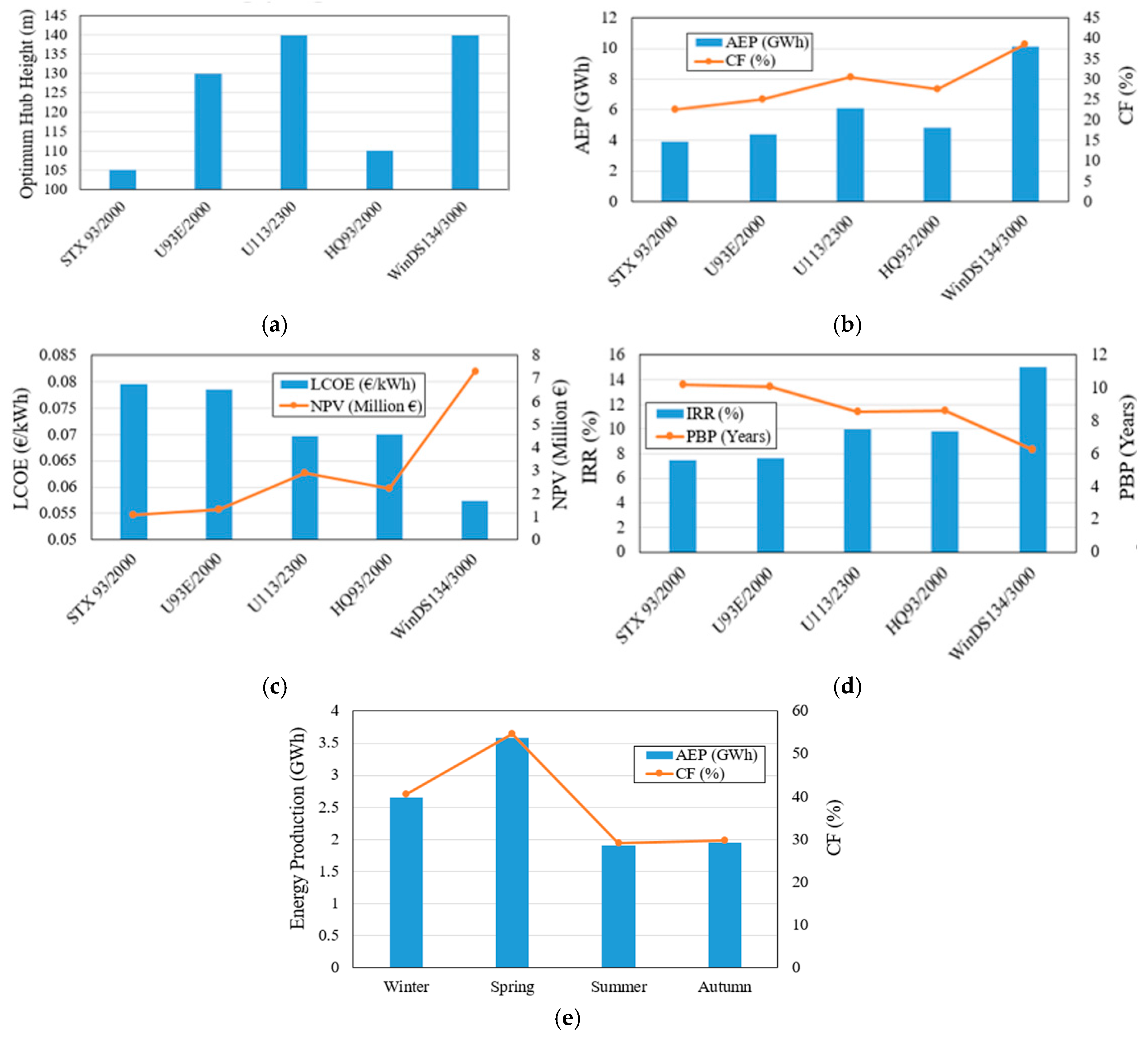
Figure 14.
Effect of hub height on wind turbines economics at discount rate of 5% for Seo-San (a) WinDS 91.3/3000; (b) HJWT 87/2000; (c) 25s 90/2500; (d) STX 72/2000; (e) U 88/2000.
Figure 14.
Effect of hub height on wind turbines economics at discount rate of 5% for Seo-San (a) WinDS 91.3/3000; (b) HJWT 87/2000; (c) 25s 90/2500; (d) STX 72/2000; (e) U 88/2000.
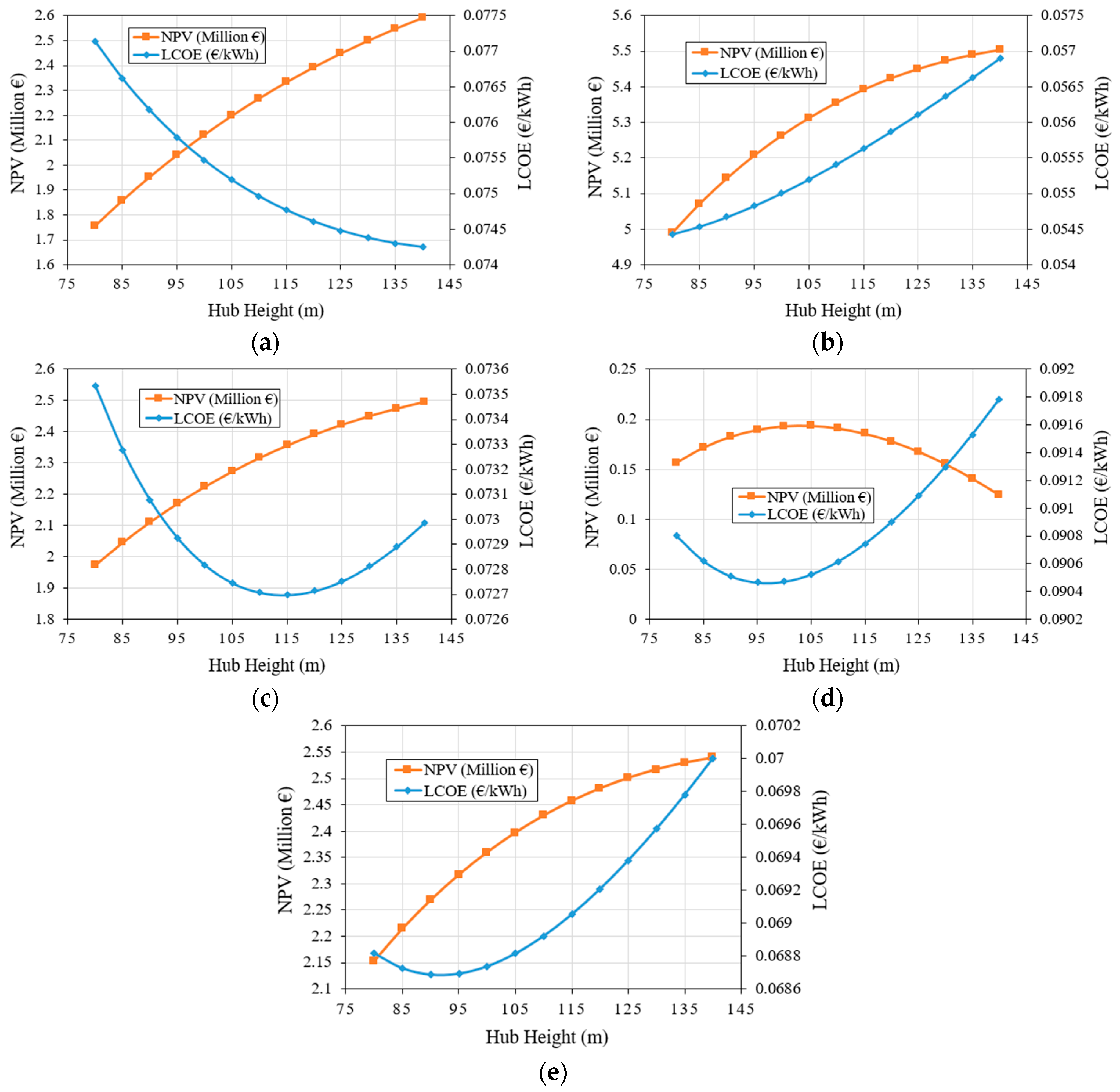
Figure 15.
Estimations of important parameters at discount rate of 5% and optimal hub height for Seo-San (a) Optimal hub height; (b) AEP & CF; (c) LCOE & NPV; (d) IRR & PBP; (e) Season-wise energy production of HJWT 87/2000.
Figure 15.
Estimations of important parameters at discount rate of 5% and optimal hub height for Seo-San (a) Optimal hub height; (b) AEP & CF; (c) LCOE & NPV; (d) IRR & PBP; (e) Season-wise energy production of HJWT 87/2000.

Table 1.
Information about the metrological masts.
| Location | Latitude | Longitude | Data Acquisition Period | Height (m) | Time Interval |
|---|---|---|---|---|---|
| Deokjeok-do | 37.22 | 126.14 | 2005–2015 | 10 | 1 h |
| Baengnyeong-do | 37.96 | 124.63 | 2001–2016 | 10 | 1 h |
| Seo-San | 36.77 | 126.49 | 1997–2016 | 10 | 1 h |
Table 2.
Long term wind data analysis of Deokjeok-do at 10 m from local ground.
| Year | Max. Speed (m/s) | Mean (m/s) | SD | k (-) | c (m/s) | T (°K) | Density (kg/m3) | WPD (W/m2) |
|---|---|---|---|---|---|---|---|---|
| 2005 | 16.5 | 4.2 | 2.7 | 1.7 | 4.7 | 284.0 | 1.243 | 47.2 |
| 2006 | 17.7 | 4.0 | 2.4 | 1.7 | 4.5 | 285.0 | 1.238 | 39.5 |
| 2007 | 17.1 | 3.9 | 2.4 | 1.7 | 4.4 | 285.3 | 1.237 | 37.5 |
| 2008 | 20.6 | 3.5 | 2.6 | 1.4 | 3.9 | 285.2 | 1.238 | 27.2 |
| 2009 | 14.8 | 2.6 | 2.3 | 1.2 | 2.8 | 285.3 | 1.237 | 11.2 |
| 2010 | 24.9 | 4.0 | 3.1 | 1.3 | 4.3 | 284.4 | 1.241 | 38.8 |
| 2011 | 27.0 | 3.8 | 3.2 | 1.2 | 4.1 | 284.7 | 1.240 | 34.4 |
| 2012 | 31.5 | 4.1 | 3.4 | 1.2 | 4.4 | 285.0 | 1.239 | 44.1 |
| 2013 | 23.4 | 3.9 | 3.2 | 1.3 | 4.2 | 285.0 | 1.239 | 36.4 |
| 2014 | 23.4 | 4.0 | 3.3 | 1.3 | 4.3 | 285.8 | 1.235 | 40.4 |
| 2015 | 18.0 | 3.8 | 2.4 | 1.6 | 4.2 | 285.6 | 1.236 | 33.1 |
| Overall Average | 21.4 | 3.8 | 2.8 | 1.4 | 4.2 | 285.0 | 1.238 | 35.4 |
Table 3.
Long term wind data analysis of Baengnyeong-do at 10 m from local ground.
| Year | Max. Speed (m/s) | Mean (m/s) | SD | k (-) | c (m/s) | T (°K) | Density (kg/m3) | WPD (W/m2) |
|---|---|---|---|---|---|---|---|---|
| 2001 | 16.0 | 4.1 | 2.3 | 1.9 | 4.6 | 284.2 | 1.242 | 41.8 |
| 2002 | 27.0 | 5.3 | 3.0 | 1.9 | 6.0 | 284.0 | 1.243 | 95.1 |
| 2003 | 20.3 | 4.8 | 2.6 | 1.9 | 5.4 | 283.4 | 1.245 | 69.7 |
| 2004 | 21.5 | 5.3 | 2.8 | 2.0 | 6.0 | 284.9 | 1.239 | 91.5 |
| 2005 | 20.9 | 5.4 | 2.8 | 2.1 | 6.1 | 284.0 | 1.243 | 99.8 |
| 2006 | 24.7 | 5.2 | 2.8 | 2.0 | 5.9 | 284.4 | 1.241 | 88.4 |
| 2007 | 24.3 | 5.0 | 2.8 | 1.9 | 5.6 | 284.8 | 1.239 | 76.2 |
| 2008 | 18.2 | 4.4 | 2.2 | 2.1 | 5.0 | 284.7 | 1.240 | 52.3 |
| 2009 | 17.6 | 4.6 | 2.4 | 2.0 | 5.1 | 284.9 | 1.239 | 58.5 |
| 2010 | 17.2 | 4.5 | 2.4 | 2.0 | 5.1 | 284.2 | 1.242 | 56.8 |
| 2011 | 21.4 | 4.3 | 2.3 | 2.0 | 4.9 | 283.5 | 1.245 | 49.5 |
| 2012 | 21.0 | 4.6 | 2.5 | 2.0 | 5.2 | 283.8 | 1.244 | 59.8 |
| 2013 | 19.8 | 4.5 | 2.3 | 2.1 | 5.1 | 283.9 | 1.244 | 58.0 |
| 2014 | 17.7 | 4.2 | 2.2 | 2.0 | 4.8 | 284.8 | 1.239 | 46.8 |
| 2015 | 17.4 | 4.1 | 2.4 | 1.8 | 4.6 | 285.1 | 1.238 | 42.1 |
| 2016 | 19.4 | 3.8 | 2.2 | 1.8 | 4.3 | 285.1 | 1.238 | 34.4 |
| Overall Average | 20.3 | 4.6 | 2.5 | 2.0 | 5.2 | 284.4 | 1.241 | 63.8 |
Table 4.
Long term wind data analysis of Seo-San at 10 m from local ground.
| Year | Max. Speed (m/s) | Mean (m/s) | SD | k (-) | c (m/s) | T (°K) | Density (kg/m3) | WPD (W/m2) |
|---|---|---|---|---|---|---|---|---|
| 1997 | 28.4 | 4.2 | 3.7 | 1.2 | 4.4 | 285.7 | 1.236 | 45.9 |
| 1998 | 30.6 | 5.2 | 4.4 | 1.2 | 5.5 | 286.4 | 1.233 | 85.6 |
| 1999 | 28.4 | 5.1 | 4.2 | 1.2 | 5.5 | 285.5 | 1.236 | 82.5 |
| 2000 | 43.0 | 5.5 | 4.6 | 1.2 | 5.9 | 284.5 | 1.241 | 103.8 |
| 2001 | 24.4 | 4.9 | 4.0 | 1.3 | 5.3 | 285.0 | 1.239 | 75.1 |
| 2002 | 32.4 | 5.6 | 4.3 | 1.3 | 6.1 | 285.0 | 1.238 | 108.4 |
| 2003 | 24.6 | 4.9 | 3.8 | 1.3 | 5.3 | 285.2 | 1.238 | 71.7 |
| 2004 | 25.4 | 5.2 | 4.2 | 1.3 | 5.5 | 285.0 | 1.238 | 84.8 |
| 2005 | 24.0 | 5.7 | 4.0 | 1.4 | 6.3 | 284.7 | 1.240 | 114.4 |
| 2006 | 25.4 | 5.5 | 4.0 | 1.4 | 6.0 | 285.4 | 1.237 | 100.8 |
| 2007 | 27.0 | 5.4 | 3.8 | 1.5 | 6.0 | 285.6 | 1.236 | 98.5 |
| 2008 | 23.6 | 5.0 | 3.9 | 1.3 | 5.5 | 285.3 | 1.237 | 78.5 |
| 2009 | 28.2 | 5.3 | 4.1 | 1.3 | 5.8 | 285.5 | 1.236 | 93.5 |
| 2010 | 46.8 | 5.5 | 4.2 | 1.3 | 6.0 | 285.0 | 1.238 | 103.3 |
| 2011 | 28.0 | 5.8 | 4.1 | 1.5 | 6.4 | 284.9 | 1.239 | 120.5 |
| 2012 | 32.0 | 4.9 | 3.8 | 1.3 | 5.4 | 284.8 | 1.239 | 74.7 |
| 2013 | 18.6 | 4.3 | 3.4 | 1.3 | 4.6 | 285.0 | 1.239 | 48.3 |
| 2014 | 19.2 | 3.7 | 3.1 | 1.2 | 3.9 | 285.6 | 1.236 | 31.0 |
| 2015 | 21.4 | 4.0 | 3.1 | 1.3 | 4.4 | 285.9 | 1.235 | 40.2 |
| 2016 | 22.0 | 4.0 | 3.1 | 1.3 | 4.3 | 286.1 | 1.234 | 38.2 |
| Overall Average | 27.7 | 5.0 | 3.9 | 1.3 | 5.4 | 285.3 | 1.237 | 80.0 |
Table 5.
IEC 61400-1 wind turbine classes.
| IEC Wind Turbine Class | ||||
|---|---|---|---|---|
| Parameter | I | II | III | S |
| Reference wind speed (m/s) | 50 | 42.5 | 37.5 | 30 |
| Annual average wind speed (m/s) | 10 | 8.5 | 7.5 | 6 |
| 50-year return gust (m/s) | 70 | 59.5 | 52.5 | 42 |
| 1-year return gust (m/s) | 52.5 | 44.6 | 39.4 | 31.5 |
Table 6.
Characteristics of selected wind turbines for Deokjeok-do and Baengnyeong-do.
| Wind Turbine Model | Manufacturer | Rated Power (MW) | Rotor Diameter (m) | IEC Wind Class | Swept Area (m2) | Power Density (m2/kW) |
|---|---|---|---|---|---|---|
| STX 93/2000 | STX Wind Power | 2 | 93.3 | IIIB | 6837 | 3.42 |
| U93E/2000 | Unison | 2 | 93 | S | 6793 | 3.4 |
| U113/2300 | Unison | 2.3 | 112.8 | S | 9994 | 4.35 |
| HQ93/2000 | Hyundai | 2 | 93 | IIIB | 6793 | 3.4 |
| WinDS134/3000 | Doosan | 3 | 134 | S | 14103 | 4.71 |
Table 7.
Characteristics of selected wind turbines for Seo-San.
| Wind Turbine Model | Manufacturer | Rated Power (MW) | Rotor Diameter (m) | IEC Wind Class | Swept Area (m2) | Power Density (m2/kW) |
|---|---|---|---|---|---|---|
| WinDS 91.3/3000 | Doosan | 3 | 91.3 | IA | 6547 | 2.19 |
| HJWT 87/2000 | Hanjin | 2 | 87 | IIA | 5945 | 2.98 |
| 25s 90/2500 | Samsung | 2.5 | 90 | IIA | 6362 | 2.55 |
| STX 72/2000 | STX Wind Power | 2 | 70.65 | IIB | 3921 | 1.97 |
| U88/2000 | Unison | 2 | 88 | IIA | 6083 | 3.05 |
Table 8.
Financial Assumptions.
| Parameter | Value |
|---|---|
| Inflation rate (%) | 3 |
| Nominal discount rate (%) | 5 |
| Corporate tax rate (%) | 25 |
| Depreciation period (Years) | 20 |
| Depreciation method | linear approximation |
| Depreciation rate (% per year) | 5 |
| Electric tariff (€/MWh) | 0.00015 |
| Operations period (Years) | 20 |
Table 9.
Wind turbine tower’s cost estimation parameters.
| Monopole-Type Foundation | |
|---|---|
| Parameter | Value |
| Steel cost (€/kg) | 0.64 |
| Steel density (kg/m3) | 7870 |
| Monopole diameter (m) | 5.5695 |
| Monopole thickness (m) | 0.075 |
Table 10.
Techno-Economic parameters at Optimum hub height in case of Deokjeok-do.
| Wind Turbine Model | Optimum Hub Height (m) | AEP (GWh) | CF (%) | LCOE (€/kWh) | NPV (Million €) | IRR (%) | PBP (Years) |
|---|---|---|---|---|---|---|---|
| STX 93/2000 | - | - | - | - | - | - | - |
| U93E/2000 | - | - | - | - | - | - | - |
| U113/2300 | - | - | - | - | - | - | - |
| HQ93/2000 | - | - | - | - | - | - | - |
| WinDS134/3000 | 140 | 6.37 | 24.26 | 0.077 | 2.07 | 8.13 | 9.72 |
© 2017 by the authors. Licensee MDPI, Basel, Switzerland. This article is an open access article distributed under the terms and conditions of the Creative Commons Attribution (CC BY) license (http://creativecommons.org/licenses/by/4.0/).
Share and Cite
MDPI and ACS Style
Ali, S.; Lee, S.-M.; Jang, C.-M. Techno-Economic Assessment of Wind Energy Potential at Three Locations in South Korea Using Long-Term Measured Wind Data. Energies 2017, 10, 1442. https://doi.org/10.3390/en10091442
AMA Style
Ali S, Lee S-M, Jang C-M. Techno-Economic Assessment of Wind Energy Potential at Three Locations in South Korea Using Long-Term Measured Wind Data. Energies. 2017; 10(9):1442. https://doi.org/10.3390/en10091442
Chicago/Turabian StyleAli, Sajid, Sang-Moon Lee, and Choon-Man Jang. 2017. "Techno-Economic Assessment of Wind Energy Potential at Three Locations in South Korea Using Long-Term Measured Wind Data" Energies 10, no. 9: 1442. https://doi.org/10.3390/en10091442
Note that from the first issue of 2016, this journal uses article numbers instead of page numbers. See further details here.