Optimal Analytical Solution for a Capacitive Wireless Power Transfer System with One Transmitter and Two Receivers


Research Group DraMCo, ESAT, Technology Campus Ghent, KU Leuven, 9000 Gent, Belgium
*
Author to whom correspondence should be addressed.
Energies 2017, 10(9), 1444; https://doi.org/10.3390/en10091444
Submission received: 24 August 2017
/
Revised: 14 September 2017
/
Accepted: 15 September 2017
/
Published: 19 September 2017
(This article belongs to the Special Issue Wireless Power Transfer and Energy Harvesting Technologies)
Abstract
:Wireless power transfer from one transmitter to multiple receivers through inductive coupling is slowly entering the market. However, for certain applications, capacitive wireless power transfer (CWPT) using electric coupling might be preferable. In this work, we determine closed-form expressions for a CWPT system with one transmitter and two receivers. We determine the optimal solution for two design requirements: (i) maximum power transfer, and (ii) maximum system efficiency. We derive the optimal loads and provide the analytical expressions for the efficiency and power. We show that the optimal load conductances for the maximum power configuration are always larger than for the maximum efficiency configuration. Furthermore, it is demonstrated that if the receivers are coupled, this can be compensated for by introducing susceptances that have the same value for both configurations. Finally, we numerically verify our results. We illustrate the similarities to the inductive wireless power transfer (IWPT) solution and find that the same, but dual, expressions apply.
1. Introduction
Wireless power transfer technologies can be divided into two categories: the far-field and near-field technologies. The former includes the transfer of energy by means of, for example, microwaves, light waves and radio waves [1,2,3,4]. The latter uses quasi-static fields to transfer the energy. Inductive wireless power transfer (IWPT) uses a time-varying magnetic field, generated by an alternating current in a coil [5]. This varying magnetic field couples the coil to another coil, enabling wireless power transfer. Magnetic resonance, which uses more than two coils, is based on the same principle [6]. IWPT technology is being applied to a broad range of applications [7].
With capacitive wireless power transfer (CWPT), energy can be transferred wirelessly by means of the electric field. Applications are the charging of, for example, electric vehicles [8], automatic guided vehicles [9], biomedical implants [10], integrated circuits [11] and low-power consumer applications [12]. Compared to IWPT, it has several advantages, such as a reduced cost and weight and the ability to transfer energy through metal [13,14]. Just as for IWPT, CWPT allows for the charging of multiple receivers at once with one transmitter. Several small receiver plates can overlay the large transmitter plates. Figure 1 shows the schematic set-up of a bipolar CWPT system with one transmitter and two receivers.
For a wireless power transfer system, two configurations are typically being pursued [15,16]. One can construct a wireless power transfer system that maximizes the amount of transferred power to the receiver, for example, for biomedical implants. The other option is to maximize the efficiency of the power transfer, for example, for the charging of electric vehicles. It is important to note that the configurations differ from each other. In this work, we analytically determine the optimal solution for both maximum power transfer and efficiency for a CWPT system with one transmitter and two receivers.
This has already been done for IWPT [17,18,19,20,21,22], but to our knowledge, it has not yet been described for CWPT. More specifically, our contributions are as follows:
- We determine analytically the optimal solution for the maximum efficiency and maximum power solution for a CWPT system with one transmitter and two receivers.
- We derive the optimal loads for each configuration and provide closed-form expressions for the maximum efficiency and power transfer.
- We demonstrate that we can compensate for coupling between the receivers by adding specific susceptances.
- We illustrate the similarities to IWPT.
2. Methodology
In this section, we first perform a circuit analysis of a general CWPT circuit with one transmitter and two receivers. Next, the maximum power and maximum efficiency solution are analytically calculated.
2.1. Circuit Analysis
A CWPT system with one transmitter and two receivers (Figure 1) can be represented by the circuit in Figure 2 [23,24]. We make an abstraction of the remote electronics (e.g., power conditioner, rectifier, etc.) to focus on the wireless link itself. On the basis of Norton’s theorem, we can represent the supply of the CWPT system with a time-harmonic current source with angular frequency . The losses in the circuit are represented by the parallel conductances , and . Wireless power transfer for two receivers may be realized by modeling the load as admittances and . The CWPT link can be described by the coupled capacitances , and [14,23,24].
The goal of the power transfer system is to wirelessly transfer power from the transmitter to both receivers. This is realized by the coupling between the transmitter capacitance and the receiver capacitances and , expressed by their mutual capacitance and , respectively. However, there can also be a coupling between the receiver capacitances and , given by . Usually, the coupling between the receivers will be negligible compared to the coupling between the transmitter and receiver, but we will nevertheless also derive the optimal solution for the non-negligible coupling . The coupling factor (i,j = 1,2,3) is defined by
In order to improve the power transfer, we construct resonant circuits by adding a shunt inductor (i = 1,2,3) to each circuit, with a value of
Instead of a shunt inductance, a series inductance can also be chosen to construct the resonant circuit. We perform the analysis for a shunt inductance, as it simplifies the calculations and allows for a better overview of the results. The methodology of our work remains the same for both topologies.
We define as the active input power, supplied by the source. and are the output powers, delivered to the loads and , respectively. We analytically determine the optimal loads and for two configurations:
- In the first configuration, we maximize the amount of power transferred from the source to the loads.
- In the second configuration, our goal is to maximize the efficiency of the system , defined by
The circuit in Figure 2 can be considered as a three-port network with peak voltage phasors and peak current phasors (i = 1,2,3) at the ports, as defined in the figure. Using Kirchhoff’s current laws, we obtain the relations between the voltages and currents of the three-port network:
Considering the three-port network, with matrices V and I defined as
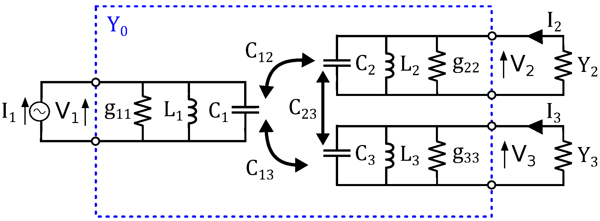
We can represent the network by an admittance matrix , indicated by the dashed rectangle in Figure 2, as
At the resonance frequency , taking into account Equation (2), the admittance matrix is given by
where we have introduced the notation for convenience.
In the next sections, we analytically determine the maximum power and maximum efficiency solution. For ease of notation, we introduce the following definitions:
2.2. Maximum Power Transfer
We determine the optimal loads (i = 2,3) to maximize the total power output of the system, where and are the load conductance and susceptance, respectively. We first consider the case in which the receivers are uncoupled.
2.2.1. Uncoupled Configuration
When the receivers are uncoupled (), the elements in the admittance matrix of Equation (9) are zero. In other words, no receiver is influenced by the presence of the other receiver. With this assumption, we can consider the system as two separate CWPT systems, each with one transmitter and one receiver. It was demonstrated in [16], using values of inductance given by Equation (2), that the optimal loads to achieve both maximum power and efficiency occur when the imaginary parts of the system equate to zero. For the configuration with uncoupled receivers, we can therefore replace the admittances and with the conductances and . We can then write
and, with Equation (8), we can write
or
Inverting the matrix allows us to find the following expressions for the voltages:
with
The input power is given by [25]:
where is the complex conjugate of . The maximum attainable power, sometimes called the “available power of the generator”, is given by [25]:
To simplify the further calculations, we use the normalized power (i = 1,2,3):
Using Equation (17), we obtain for the normalized input power :
We find the loads to obtain the maximum power transfer:
Substituting these conductances into Equations (26) and (27) results in the maximum normalized output power :
Analogously, we obtain the corresponding normalized input power in this maximum power configuration:
From Equation (3), we obtain the corresponding efficiency:
2.2.2. Coupled Configuration
We now consider the case in which the receivers are coupled (). The only difference to the uncoupled case is that the elements in the admittance matrix (9) are non-zero. Because this only adds purely imaginary elements to the admittance matrix , the real part of the maximum power solution for the loads equals that for the uncoupled case. Adding appropriate susceptances to the circuit allows us to compensate for the extra purely imaginary elements, resulting in the same maximum power output (Equation (32)) for the same conductances and as for the uncoupled configuration. We then determine the values for these susceptances.
We consider the circuit of Figure 3. and are the susceptances added to compensate for the non-zero coupling between and . The admittance matrix of the three-port network that includes and is given by
Equation (16) now becomes
Inverting the matrix allows us to find the following expressions for the voltages:
with
We note that the above equations reduce to the expressions for the uncoupled configuration when , and are equal to zero. In order to compensate for the coupling between and , Equations (37)–(39) for the voltages of the three-port network have to be the same as the relations for the uncoupled configurations, that is, Equations (17)–(19), respectively. By analytically solving the system of equations thus obtained for and , we find a unique solution:
Substituting and with the values for and , we obtain
Because the susceptances and are positive, they correspond to capacitances and , respectively, given by
We note that, as expected, the compensating capacitances and become zero when there is no coupling present between the receivers (i.e., ).
Because and compensate for the coupling between and , the input and output power and the efficiency are the same as the values for the uncoupled configuration. An overview can be found in the second column of Table 1.
2.3. Maximum Efficiency
We determine the optimal loads and to maximize the efficiency of the total system, as defined in Equation (3). We first consider the case in which the receivers are uncoupled.
2.3.1. Uncoupled Configuration
When the receivers are uncoupled (), the elements in the admittance matrix (Equation (9)) are zero. The optimal loads are again purely real [16]: and .
We find
We derive to and and equate to zero:
We find the values for the conductances and for the maximum efficiency configuration:
2.3.2. Coupled Configuration
We now consider the case in which the receivers are coupled (). With the same reasoning as for the maximum power configuration, we can add susceptibilities and to compensate for the coupling between and . The derivation for calculating the values of and is identical to the maximum power configuration until arriving at Equations (41) and (42). We then substitute and with the values for and .
We obtain for the maximum efficiency configuration the same compensating capacitances as for the maximum power configuration:
This is to be expected. The goal of the added susceptances and is to compensate for the coupling between the receivers, in any configuration, whether it is to achieve maximum power transfer, maximum efficiency, or any other configuration. In other words, achieving the maximum power transfer or maximum efficiency for a given CWPT system with one transmitter and two receivers only requires us to change the real part of the load of the receivers. The compensating capacitances and are the same for both configurations.
The maximum attainable efficiency , in the uncoupled case as well as in the coupled case, when applying and as loads, is given by
Substituting and into Equation (24) results in the normalized input power :
An overview of the different values can be found in Table 1.
3. Discussion
In this section, we first numerically verify our results. Next, we analyze the maximum power and maximum efficiency solution in more detail, and illustrate the similarities with IWPT.
3.1. Numerical Verification
First, we notice that, if one receiver is absent or uncoupled (e.g., ), the results of Table 1 correspond to the solutions for a CWPT system with one transmitter and one receiver [16].
We now verify the above analytical derivation by circuit simulation. We consider the system of Figure 2 with one transmitter and two capacitive coupled receivers. If we assume a system composed of a large aluminum transmitter with aluminum receiver plates of 10 cm × 10 cm, coated with polyethylene as a dielectric material, at a distance of 2.5 mm between transmitter and receiver, we can assume the representative values of Table 2 [14,24].
Using Equations (1), (2), and (10)–(12), the values of the coupling factors, resonance inductances, and auxiliary variables are calculated (Table 3).
We first verify the optimal loads for the maximum power configuration. From Table 1, we calculate the following:
- The optimal loads and for achieving maximum power transfer.
- The capacitances and , necessary to compensate for the coupling between both receivers.
- The corresponding normalized input and output power.
- The efficiency of the system.
The calculated values are listed in Table 4.
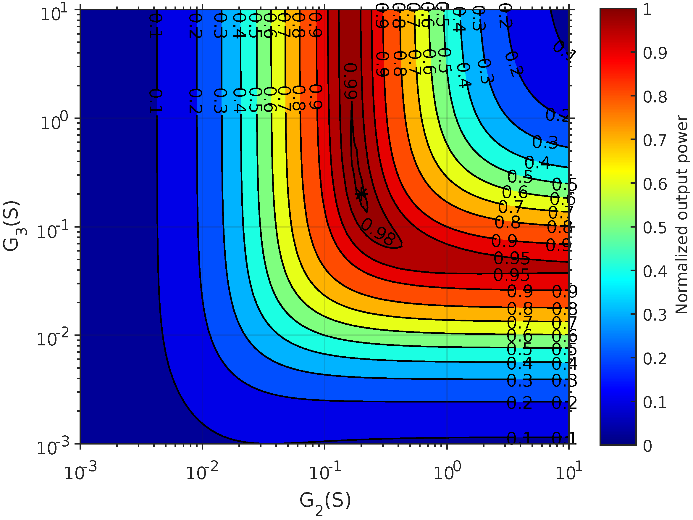
This system was simulated in SPICE for varying loads and . Figure 4 shows the normalized power output . A maximum of 0.992 was obtained at the loads and of 189 and 252 mS, respectively. This was in accordance with the analytical result from Table 4. Additionally, the obtained efficiency of 49.2% at this point corresponded with the analytical calculated value.
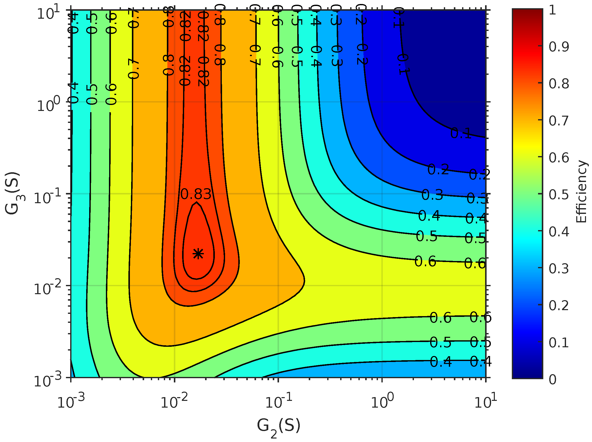
Secondly, we consider the maximum efficiency configuration for the same system. From Table 1, we find the values listed in Table 4. By SPICE simulation, we calculated the efficiency of the system for varying loads and (Figure 5). A maximum efficiency of 83.6% was achieved at the loads and of 16.8 and 22.5 mS, respectively, which was in accordance with the analytical derived result. The corresponding normalized output power was 0.298, corresponding with the expected value (Table 4).
Finally, we verify that the calculated values of the capacitances and indeed compensate for the coupling between the receivers. We simulated both the maximum power and the maximum efficiency configuration for the uncoupled configuration; we considered the same system as described by Table 2, but now with equal to zero and no compensating capacitances and present. We obtained the same calculated values of the coupled scenario (Table 3 and Table 4). Circuit simulations with SPICE produced the same results as in Figure 4 and Figure 5, indicating that and indeed compensate for the coupling between the receivers.
3.2. Analysis of the Results
From Table 1, it can be seen that the optimal conductances for the maximum power configuration are always larger than for the maximum efficiency configuration, as . Additionally, the normalized input power is higher in the maximum power scenario than in the maximum efficiency scenario. From Figure 4 and Figure 5, it can be seen that for the numerical example, both the output power and efficiency are near the maximum, which varies more when changing than when changing . The reason is that the coupling between the transmitter and the first receiver is higher than the coupling between the transmitter and the second receiver. A further, more detailed analysis is beyond the scope of this work.
In our numerical example, the coupling factor between both receivers is 22%, that is, . We demonstrated that capacitances and are necessary to compensate for this coupling between the receivers.
We illustrate the influence of the presence of these compensating capacitances with an example. We calculate the normalized output power and the efficiency for non-ideal loads of = 1 mS and = 10 mS. The normalized output power with compensating capacitances and is 0.0376. If no compensating capacitances are present, is 0.0246, about 7% lower. The efficiency with and without compensating capacitances is 50.8% and 41.5%, respectively, an absolute difference of 9.3%.
In the neighborhood of the maximum power point and maximum efficiency point, the difference between and , respectively, is negligible for the circuit with and without compensating capacitances for this example.
An important limitation of our proposed model is that it is restricted to static CWPT set-ups. The model assumes that all elements, including the coupled capacitances, are lumped elements and are fixed, whereas in reality, the capacitances are distributed elements and are dependent on the position of the receivers. For the implementation of our model, the values of the capacitances and coupling coefficients can be determined by measurement [24]. However, these values are not fixed. Indeed, the values of the capacitances and coupling coefficients are not independent of each other [24]. For example, a change in the position of one receiver will not only influence the coupling coefficients for that receiver, but also the values of the capacitances. Even the value of the capacitance of the transmitter and the value of the coupling coefficient between the transmitter and the second receiver can vary as a result of the change in position of the first receiver. This implies that our model is only valid for static applications, for example, the charging of space-confined systems, such as low-power consumer applications [12] or three-dimensional integrated circuits [11], for which the receivers have predefined locations. For moving receivers, such as electric vehicles [26], robot arms and in-track-moving systems [12], our model is not valid. For future work, we plan to extend our model by applying distributed elements.
3.3. Duality to IWPT
Given the duality principle in network theory [25], which finds its origin in the symmetry of Maxwell’s equation for the electric and magnetic fields, parallels can be drawn between CWPT and IWPT. Table 5 gives an overview of the relevant dual quantities for CWPT and IWPT.
The dual network of Figure 3 is given in Figure 6. A transmitter is supplied by a voltage source . The inductances (i = 1,2,3) are coupled and expressed by their mutual inductance ; the coupling factor is defined as
The loads of the two receivers are and . Resonance capacitors and resistances (i = 1,2,3) are added in series to each circuit. The reactances and compensate for the coupling between and . Just as for the CWPT set-up, this circuit is limited to static set-ups and does not include, for example, the leakage flux in the primary circuit.
Given the duality principle, we can for IWPT define the following analogous variables:
With these definitions and by applying the duality principle, we obtain the quantities of Table 6, analogous to in [17,18,19]. We notice the similarities for the corresponding quantities for CWPT in Table 1. For example, the load conductance for CWPT is given by and for the maximum power and efficiency configuration, respectively. The dual load for IWPT, the resistance , is given by and for the maximum power and efficiency configuration, respectively, which corresponds to the dual values of CWPT. Analogously, for CWPT, the elements that compensate for the receiver’s coupling are susceptances, whereas for IWPT, they are reactance elements given by the same, but dual, expressions of CWPT.
4. Conclusions
We determined analytically the closed-form expressions for a CWPT system with one transmitter and two receivers for two relevant configurations: (i) maximum power transfer, and (ii) maximum system efficiency. The results are summarized in Table 1. We also determined the susceptances to compensate for coupling between the receivers and demonstrated that they remain unaltered for both configurations. We numerically verified our results and, using the duality principle of network theory, illustrated the similarities with the analogue IWPT system.
Acknowledgments
This work was executed within MoniCow, a research project bringing together academic researchers and industry partners. The MoniCow project was co-financed by imec (iMinds) and received project support from Flanders Innovation & Entrepreneurship.
Author Contributions
Ben Minnaert initiated the study, performed the calculations and conducted the simulations. Nobby Stevens provided the general supervision of the calculations and simulations. Ben Minnaert wrote the manuscript. Nobby Stevens commented on and revised the manuscript.
Conflicts of Interest
The authors declare no conflict of interest.
Abbreviations
The following abbreviations are used in this manuscript:
| IWPT | Inductive wireless power transfer |
| CWPT | Capacitive wireless power transfer |
References
- Lu, X.; Wang, P.; Niyato, D.; Kim, D.I.; Han, Z. Wireless charging technologies: Fundamentals, standards, and network applications. IEEE Commun. Surv. Tutor. 2016, 18, 1413–1452. [Google Scholar] [CrossRef]
- Shinohara, N. Wireless Power Transfer via Radiowaves; John Wiley & Sons: New York, NY, USA, 2014. [Google Scholar]
- Huang, K.; Zhou, X. Cutting the last wires for mobile communications by microwave power transfer. IEEE Commun. Mag. 2015, 53, 86–93. [Google Scholar] [CrossRef] [Green Version]
- Rabie, K.M.; Adebisi, B.; Rozman, M. Outage probability analysis of WPT systems with multiple-antenna access point. In Proceedings of the IEEE 10th International Symposium on Communication Systems, Networks and Digital Signal Processing (CSNDSP), Prague, Czech Republic, 20–22 July 2016. [Google Scholar]
- Mou, X.; Sun, H. Wireless power transfer: Survey and roadmap. In Proceedings of the 81st IEEE Vehicular Technology Conference (VTC Spring), Glasgow, UK, 11–14 May 2015; pp. 1–5. [Google Scholar]
- Rozman, M.; Fernando, M.; Adebisi, B.; Rabie, K.M.; Kharel, R.; Ikpehai, A.; Gacanin, H. Combined Conformal Strongly-Coupled Magnetic Resonance for Efficient Wireless Power Transfer. Energies 2017, 10, 498. [Google Scholar] [CrossRef]
- Carvalho, N.B.; Georgiadis, A.; Costanzo, A.; Stevens, N.; Kracek, J.; Pessoa, L.; Roselli, L.; Dualibe, F.; Schreurs, D.; Mutlu, S.; et al. Europe and the future for WPT: European contributions to wireless power transfer technology. IEEE Microw. Mag. 2017, 18, 56–87. [Google Scholar] [CrossRef]
- Dai, J.; Ludois, D.C. Wireless electric vehicle charging via capacitive power transfer through a conformal bumper. In Proceedings of the IEEE Applied Power Electronics Conference and Exposition (APEC), Charlotte, NC, USA, 15–19 March 2015; pp. 3307–3313. [Google Scholar]
- Miyazaki, M.; Abe, S.; Suzuki, Y.; Sakai, N.; Ohira, T.; Sugino, M. Sandwiched parallel plate capacitive coupler for wireless power transfer tolerant of electrode displacement. In Proceedings of the IEEE MTT-S International Conference on Microwaves for Intelligent Mobility (ICMIM), Nagoya, Japan, 19–21 March 2017; pp. 29–32. [Google Scholar]
- Sodagar, A.M.; Amiri, P. Capacitive coupling for power and data telemetry to implantable biomedical microsystems. In Proceedings of the 4th International IEEE/EMBS Conference on Neural Engineering, Antalya, Turkey, 29 April–2 May 2009; pp. 411–414. [Google Scholar]
- Culurciello, E.; Andreou, A.G. Capacitive inter-chip data and power transfer for 3-D VLSI. IEEE Trans. Circuits Syst. II Express Briefs 2006, 53, 1348–1352. [Google Scholar] [CrossRef]
- Theodoridis, M.P. Effective capacitive power transfer. IEEE Trans. Power Electron. 2012, 27, 4906–4913. [Google Scholar] [CrossRef]
- Jawad, A.M.; Nordin, R.; Gharghan, S.K.; Jawad, H.M.; Ismail, M. Opportunities and Challenges for Near-Field Wireless Power Transfer: A Review. Energies 2017, 10, 1022. [Google Scholar] [CrossRef]
- Minnaert, B.; Stevens, N. Conjugate image theory applied on capacitive wireless power transfer. Energies 2017, 10, 46. [Google Scholar] [CrossRef]
- Monti, G.; Costanzo, A.; Mastri, F.; Mongiardo, M. Optimal design of a wireless power transfer link using parallel and series resonators. Wirel. Power Transf. 2016, 3, 105–116. [Google Scholar] [CrossRef]
- Dionigi, M.; Mongiardo, M.; Monti, G.; Perfetti, R. Modelling of wireless power transfer links based on capacitive coupling. Int. J. Numer. Model. 2017, 30. [Google Scholar] [CrossRef]
- Monti, G.; Che, W.; Wang, Q.; Costanzo, A.; Dionigi, M.; Mastri, F.; Mongiardo, M.; Perfetti, R.; Tarricone, L.; Chang, Y. Wireless Power Transfer With Three-Ports Networks: Optimal Analytical Solutions. IEEE Trans. Circuits Syst. I Regul. Pap. 2016, 64, 494–503. [Google Scholar] [CrossRef]
- Monti, G.; Che, W.; Wang, Q.; Dionigi, M.; Mongiardo, M.; Perfetti, R.; Chang, Y. Wireless power transfer between one transmitter and two receivers: optimal analytical solution. Wirel. Power Transf. 2016, 3, 63–73. [Google Scholar] [CrossRef]
- Mongiardo, M.; Wang, Q.; Che, W.; Dionigi, M.; Perfetti, R.; Chang, Y.; Monti, G. Wireless power transfer between one transmitter and two receivers: Optimal analytical solution. In Proceedings of the IEEE Asia-Pacific Microwave Conference (APMC), Nanjing, China, 6–9 December 2015; pp. 1–3. [Google Scholar]
- Zhang, T.; Fu, M.; Ma, C.; Zhu, X. Optimal load analysis for a two-receiver wireless power transfer system. In Proceedings of the IEEE Wireless Power Transfer Conference (WPTC), Jeju, South Korea, 8–9 May 2014; pp. 84–87. [Google Scholar]
- Ean, K.K.; Chuan, B.T.; Imura, T.; Hori, Y. Impedance matching and power division algorithm considering cross coupling for wireless power transfer via magnetic resonance. In Proceedings of the IEEE 34th International Telecommunications Energy Conference (INTELEC), Scottsdale, AZ, USA, 30 September–4 October 2012; pp. 1–5. [Google Scholar]
- Zhong, C.; Luo, B.; Ning, F.; Liu, W. Reactance compensation method to eliminate cross coupling for two-receiver wireless power transfer system. IEICE Electron. Express 2015, 12, 1–10. [Google Scholar] [CrossRef]
- Hong, J.S.G.; Lancaster, M.J. Microstrip Filters for RF/Microwave Applications, 1st ed.; John Wiley & Sons: New York, NY, USA, 2001; pp. 235–253. [Google Scholar]
- Huang, L.; Hu, A.P. Defining the mutual coupling of capacitive power transfer for wireless power transfer. Electron. Lett. 2015, 51, 1806–1807. [Google Scholar] [CrossRef]
- Montgomery, C.G.; Dicke, R.H.; Purcell, E.M. Principles of Microwave Circuits; McGraw-Hill Book Company: New York, NY, USA, 1948. [Google Scholar]
- Vincent, D.; Sang, P.H.; Williamson, S.S. Feasibility study of hybrid inductive and capacitive wireless power transfer for future transportation. In Proceedings of the IEEE Transportation Electrification Conference and Expo (ITEC), Chicago, IL, USA, 22–24 June 2017. [Google Scholar]
Figure 1.
Schematic overview of a capacitive wireless power transfer (CWPT) system with one transmitter and two receivers.
Figure 1.
Schematic overview of a capacitive wireless power transfer (CWPT) system with one transmitter and two receivers.
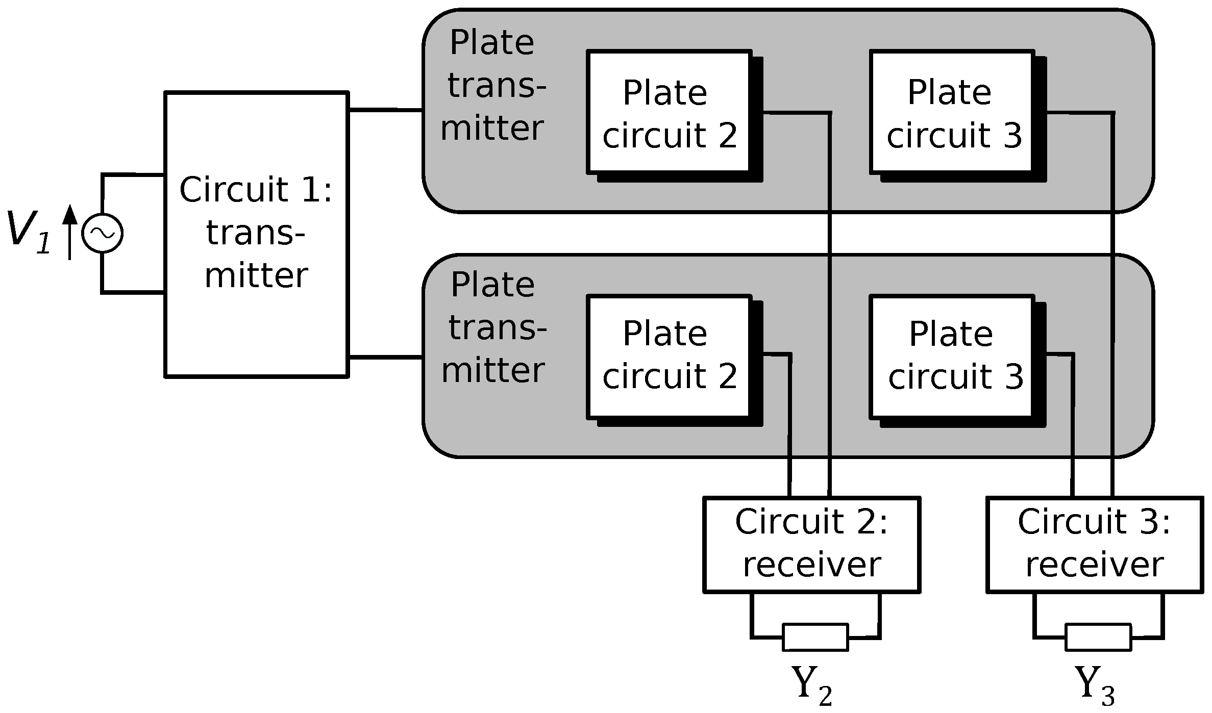
Figure 2.
Equivalent circuit to a capacitive wireless power transfer (CWPT) system with one transmitter and two receivers.
Figure 2.
Equivalent circuit to a capacitive wireless power transfer (CWPT) system with one transmitter and two receivers.

Figure 3.
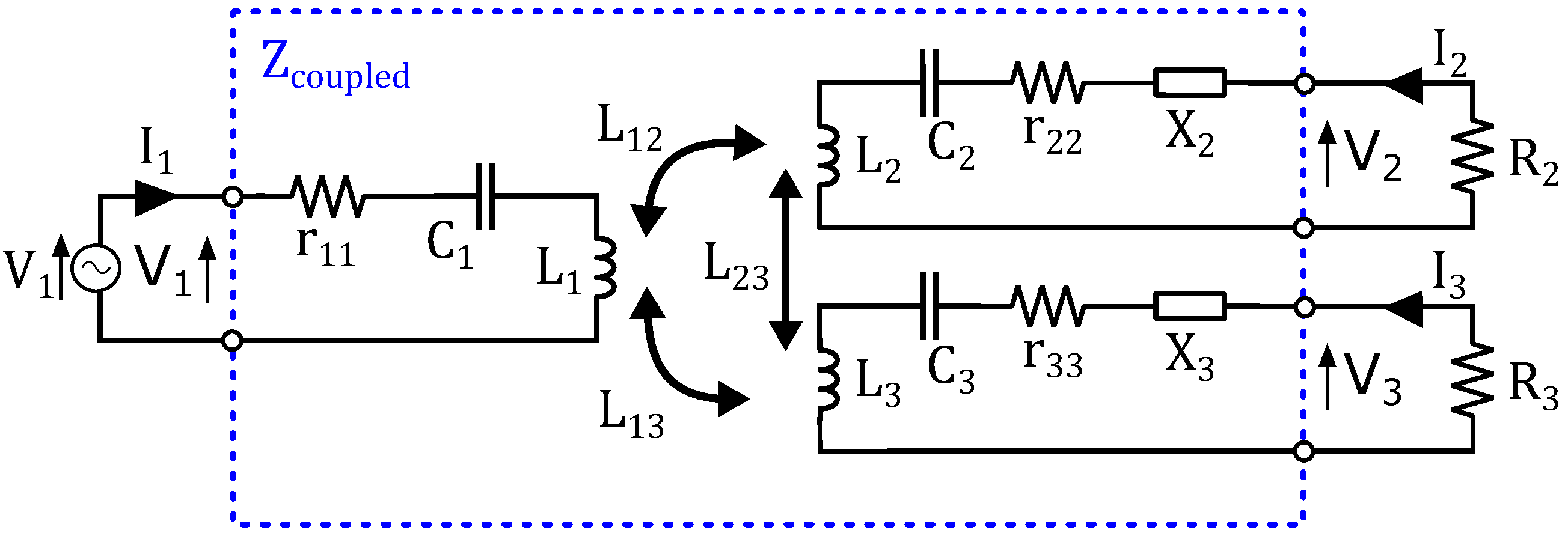
Schematic overview of a capacitive wireless power transfer (CWPT) system with one transmitter and two receivers, where we have added the susceptances and to compensate for the coupling between and . The dashed rectangle indicates the three-port network characterized by the admittance matrix .
Figure 3.
Schematic overview of a capacitive wireless power transfer (CWPT) system with one transmitter and two receivers, where we have added the susceptances and to compensate for the coupling between and . The dashed rectangle indicates the three-port network characterized by the admittance matrix .
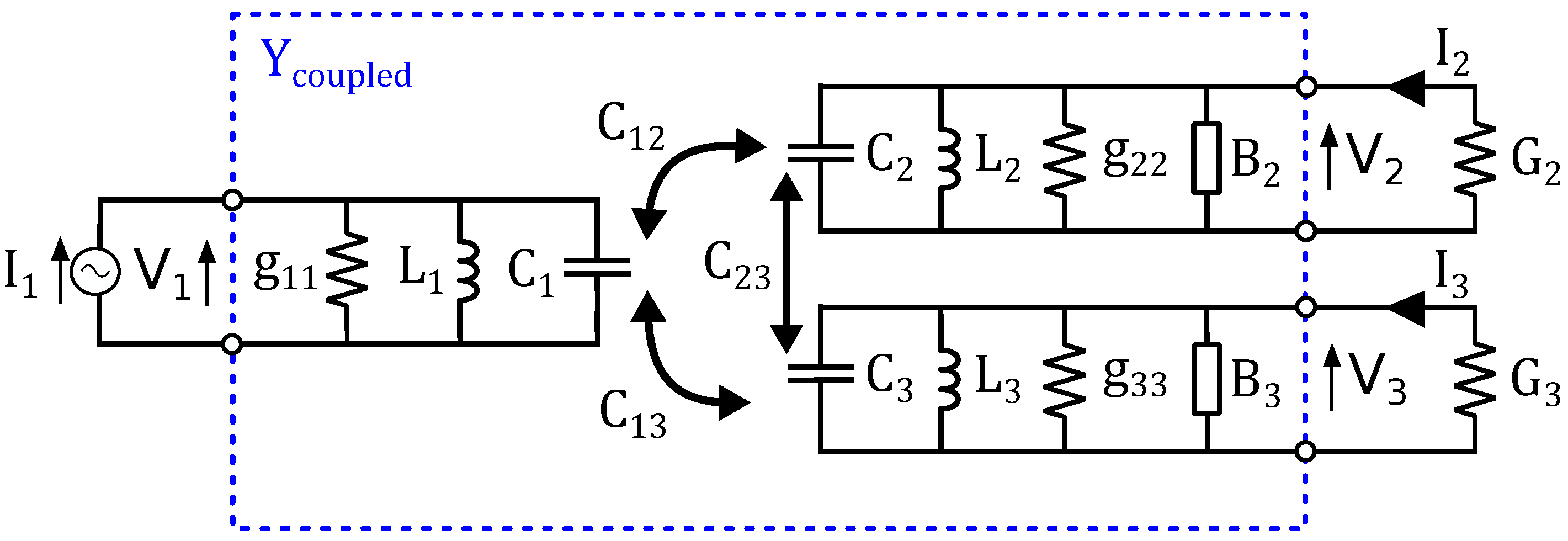
Figure 4.
The normalized output power as a function of the load conductances and for the capacitive wireless power transfer (CWPT) system with one transmitter and two receivers of Table 2. The asterisk indicates the location of the maximum normalized output power of 0.992.
Figure 4.
The normalized output power as a function of the load conductances and for the capacitive wireless power transfer (CWPT) system with one transmitter and two receivers of Table 2. The asterisk indicates the location of the maximum normalized output power of 0.992.

Figure 5.
The efficiency as a function of the load conductances and for the capacitive wireless power transfer (CWPT) system with one transmitter and two receivers of Table 2. The asterisk indicates the location of the maximum efficiency of 83.6%.
Figure 5.
The efficiency as a function of the load conductances and for the capacitive wireless power transfer (CWPT) system with one transmitter and two receivers of Table 2. The asterisk indicates the location of the maximum efficiency of 83.6%.

Figure 6.
Schematic overview of an inductive wireless power transfer (IWPT) system with one transmitter and two receivers, with the reactances and to compensate for the coupling between and . The dashed rectangle indicates the three-port network characterized by the impedance matrix .
Figure 6.
Schematic overview of an inductive wireless power transfer (IWPT) system with one transmitter and two receivers, with the reactances and to compensate for the coupling between and . The dashed rectangle indicates the three-port network characterized by the impedance matrix .


Table 1.
Overview of the different quantities for the maximum power and the maximum efficiency solution.
Table 1.
Overview of the different quantities for the maximum power and the maximum efficiency solution.
| Quantity | Maximum Power Configuration | Maximum Efficiency Configuration |
|---|---|---|
Table 2.
For the circuit simulation, we consider the following values for a capacitive wireless power transfer (CWPT) system with one transmitter and two receivers.
Table 2.
For the circuit simulation, we consider the following values for a capacitive wireless power transfer (CWPT) system with one transmitter and two receivers.
| Quantity | Value | Quantity | Value |
|---|---|---|---|
| 1.0 mS | 2.0 mS | ||
| 1.5 mS | f | 10 MHz | |
| 300 pF | 200 pF | ||
| 250 pF | 100 pF | ||
| 200 pF | 50 pF |
Table 3.
Calculated values for the considered capacitive wireless power transfer (CWPT) system.
| Quantity | Value | Quantity | Value |
|---|---|---|---|
| 0.84 H | 73% | ||
| 1.01 H | 41% | ||
| 1.27 H | 22% | ||
| 10.3 | 11.2 | ||
| 4.44 | - | - |
Table 4.
Calculated values for the considered capacitive wireless power transfer (CWPT) system for the maximum power and the maximum efficiency configuration.
Table 4.
Calculated values for the considered capacitive wireless power transfer (CWPT) system for the maximum power and the maximum efficiency configuration.
| Quantity | Maximum Power Configuration | Maximum Efficiency Configuration |
|---|---|---|
| 189 mS | 16.8 mS | |
| 252 mS | 22.5 mS | |
| 18.8 pF | 18.8 pF | |
| 133 pF | 133 pF | |
| 2.02 | 0.356 | |
| 0.992 | 0.298 | |
| 49.2% | 83.6% |
Table 5.
Dual quantities between capacitive wireless power transfer (CWPT) and inductive wireless power transfer (IWPT).
Table 5.
Dual quantities between capacitive wireless power transfer (CWPT) and inductive wireless power transfer (IWPT).
| CWPT | IWPT |
|---|---|
| Current, I | Voltage, V |
| Admittance, Y | Impedance, Z |
| Conductance, G | Resistance, R |
| Susceptance, B | Reactance, X |
| Parallel | Series |
Table 6.
Overview of the different quantities for the maximum power and the maximum efficiency solution for an inductive wireless power transfer (IWPT) system with one transmitter and two receivers.
Table 6.
Overview of the different quantities for the maximum power and the maximum efficiency solution for an inductive wireless power transfer (IWPT) system with one transmitter and two receivers.
| Quantity | Maximum Power Configuration | Maximum Efficiency Configuration |
|---|---|---|
© 2017 by the authors. Licensee MDPI, Basel, Switzerland. This article is an open access article distributed under the terms and conditions of the Creative Commons Attribution (CC BY) license (http://creativecommons.org/licenses/by/4.0/).
Share and Cite
MDPI and ACS Style
Minnaert, B.; Stevens, N. Optimal Analytical Solution for a Capacitive Wireless Power Transfer System with One Transmitter and Two Receivers. Energies 2017, 10, 1444. https://doi.org/10.3390/en10091444
AMA Style
Minnaert B, Stevens N. Optimal Analytical Solution for a Capacitive Wireless Power Transfer System with One Transmitter and Two Receivers. Energies. 2017; 10(9):1444. https://doi.org/10.3390/en10091444
Chicago/Turabian StyleMinnaert, Ben, and Nobby Stevens. 2017. "Optimal Analytical Solution for a Capacitive Wireless Power Transfer System with One Transmitter and Two Receivers" Energies 10, no. 9: 1444. https://doi.org/10.3390/en10091444
Note that from the first issue of 2016, this journal uses article numbers instead of page numbers. See further details here.