Machine Learning for Wind Turbine Blades Maintenance Management


1
Ingenium Research Group, Castilla-La Mancha University, 13071 Ciudad Real, Spain
2
Ingeniería Industrial y Aeroespacial, Universidad Europea Madrid, Villaviciosa de Odón, 28670 Madrid, Spain
*
Author to whom correspondence should be addressed.
Energies 2018, 11(1), 13; https://doi.org/10.3390/en11010013
Submission received: 28 October 2017
/
Revised: 14 December 2017
/
Accepted: 18 December 2017
/
Published: 21 December 2017
(This article belongs to the Collection Wind Turbines)
Abstract
:Delamination in Wind Turbine Blades (WTB) is a common structural problem that can generate large costs. Delamination is the separation of layers of a composite material, which produces points of stress concentration. These points suffer greater traction and compression forces in working conditions, and they can trigger cracks, and partial or total breakage of the blade. Early detection of delamination is crucial for the prevention of breakages and downtime. The main novelty presented in this paper has been to apply an approach for detecting and diagnosing the delamination WTB. The approach is based on signal processing of guided waves, and multiclass pattern recognition using machine learning. Delamination was induced in the WTB to check the accuracy of the approach. The signal is denoised by wavelet transform. The autoregressive Yule–Walker model is employed for feature extraction, and Akaike’s information criterion method for feature selection. The classifiers are quadratic discriminant analysis, k-nearest neighbors, decision trees, and neural network multilayer perceptron. The confusion matrix is employed to evaluate the classification, especially the receiver operating characteristic analysis by: recall, specificity, precision, and F-score.
1. Introduction
Wind energy is a clean resource, and one that is growing worldwide, since it is the most efficient renewable energy source [1,2]. Wind turbines present structural health problems, mainly in Wind Turbine Blades (WTB) [3]. Delamination is one of the most common problems in composite materials, caused by the disunion of their layers or by the detachment of their adhesive bonds. Low speed impact on working conditions can create a visible fault on WTB [4,5]. The microstructural fault increases because of the cyclic fatigue loads, and it can degrade the rigidity and strength of the composite [6]. Similarly, delamination can be generated by an error in the manufacturing process.
State space models are employed to predict the growth of delamination by stress/strain, fracture mechanic, cohesive zone, extended finite element method based models [7]. Hoon Sohn et al. used a wavelet-based signal processing technique, together with an active sensing system, to detect delamination in near-real-time for composite structures [8].
Smart blades are currently used in Structural and Health Monitoring (SHM) systems and applied to WTB, using sensors in the blades to monitor the condition of the WTB. McGugan et al. propose a technique for measuring and evaluating the structural integrity by introducing a new concept of tolerance to damage. It involves the life cycle of a blade, i.e., design, operation, maintenance, repair, and recycling. Pattern recognition is used to establish a “damages map” that evaluates the SHM, allowing an efficient operation of the wind turbine in terms of load relief, limited maintenance, and repairs [9,10]. Dynamic models are also employed in SHM to detect instantaneous structural changes online [11,12]. Sohn et al. propose an approach composed of four steps [13]: operational evaluation; data acquisition & cleansing; feature extraction & data reduction; and statistical model development. The Artificial Neural Networks (ANN) model produces accurate results in terms of fault diagnosis. ANN demonstrates advantages, such as speed, simplicity, and robustness [14]. Rasit Ata presents a review of ANN applied in wind energy systems [15]. Bork et al. [16,17], Yam et al. [18], and Su and Ye [19] have issued different approaches considering Lamb waves and ANN.
Ultrasonic Lamb waves have been employed in this paper to detect and diagnose faults. Lamb waves can detect internal and surface faults in WTB [20,21]. A wide range of potential defects that employ different algorithms are studied in the literature [22,23]. In this paper, Discrete Wavelet Transforms (DWT) are applied to filter signals. DWT is effective for signal denoising, filtration, compression, and feature extraction of signals [24]. A correct signal pre-processing, or an appropriate selection of characteristics, can result in a simple classifier obtaining excellent results [25]. The Daubechies wavelet family was employed in this paper. It has been demonstrated that it is sensitive to sudden changes [26]. The normalization of the signals regarding the environmental and operational conditions is a key issue in avoiding false diagnosis [27]. The mean value of the time series has been used to remove the direct current offset from the signal. This result is divided by the standard deviation of the signal to normalize varying amplitudes in the signal. Gómez et al. developed a similar pattern recognition approach for diagnosing ice on WTB by employing Daubechies wavelet [21,28].
The main purposes of Feature Extraction (FE) and Feature Selection (FS) in this paper are to reduce dimensionality, and to increase computational performance and classifier accuracy. The Auto-Regressive (AR) method is proposed to extract the FE. The AR model has high sensitivity to damage features [29,30,31]. This technique has been employed in time series analysis and predictive models for fault detection [32,33], but it has not been studied enough for pattern recognition. Yao et al. applied statistical algorithms of pattern recognition using AR FE techniques by spectral model and residual AR with acceleration data [34]. Nardi et al. studied delamination by means of AR models [35]. Figueiredo et al. [36] propose an AR-based approach using acceleration time series in order to distinguish variations in characteristics related to damage from those related to operational and environmental effects. In this paper, selection of the number of AR model parameters is carried out. A higher order model can fit the dataset, but cannot be generalized to other datasets. A lower model order may not adequately represent the physical dynamics of the system.
FS is employed to set the architecture of the ANN. The number of inputs corresponds to the features selected, the outputs (number of class) to the network conditions, and the number of nodes in the hidden layer depend on the features and classes.
Akaike’s Information Criteria (AIC) [37], Final Prediction Error (FPE) criterion [38], Partial Autocorrelation Function (PAF) [39], Root Mean Square (RMS) [40] and Singular Value Decomposition (SVD) [41] have been employed in this paper to obtain the most suitable AR model by choosing the number of parameters. The results of this work suggest that the optimal order is from 15 to 30.
The ultrasonic waves are analyzed by signal processing and classifiers by Machine Learning (ML) and ANN to determine the degree of delamination. The experiments consider six levels of delamination. This study analyses different classifiers of ML and ANN to obtain the best success rate.
The classifiers used to identify the scenarios are quadratic discriminant analysis [42], k-nearest neighbors [43], and decision trees [44]. The confusion matrix is employed to evaluate the classification using the receiver operating characteristic analysis by: recall, specificity, precision and F-score. The conventional methods to establish the average performance in all categories were macro and micro average. The recommendations by Demšar, and Garcia and Herrera have been used to compare the classifiers and analyze their results. The Friedman test has been used to test the null hypothesis that all classifiers achieve the same average. The Bonferroni–Dunn test has been applied to determine significant differences between the top-ranked classifier and the next one. The Holm test was applied to contrast the results. When this approach was used, all the scenarios showed a high level of accuracy.
The main novelty is to employ the abovementioned approach for fault detection and diagnosis in WTB that employs guided waves, where it has not been found in literature for detecting delamination in WTB.
2. Approach for Delamination, Detection, and Diagnosis in WTB
The ultrasonic signal studied should be conditioned and denoised to train the classifiers properly [45]. The wavelet transform has been used in this paper to perform signal denoising [46,47].
The inputs and training patterns are critical in the design of the classifiers, because they will determine the performance of the network and its architecture. It is necessary to use a technique that reduces the number of inputs that maintain the characteristic information of the signal. The feature coefficients of each ultrasonic signal are extracted using the AR model by the Yule–Walker method [48].
The classifiers considered in ML are: Decision Tree (DT), Quadratic Discriminant Analysis (QDA), K-Nearest Neighbors (KNN), and neural network multilayer perceptron. The schematized process of the approach is shown in Figure 1.
The wavelet threshold denoising method is applied by employing a multilevel 1D wavelet analysis by Daubechies family [49,50]. The wavelet decomposition structure of the signal is extracted. The threshold for the denoising is obtained by the wavelet coefficients selection rule using a penalization method provided by Birgé-Massart [51,52].
Each set of ultrasonic signals of every delamination level is averaged and normalized by Equation (1) to avoid false positive damage:
where is the normalized signal, is the mean, and is the standard deviation of y.
In an AR model of order p, the current output is a linear combination of the last p output plus a white noise input. The weight on the last p output minimizes the mean square prediction error of the AR model. If y(t) is the current value of the output, and y(t) presents a zero-mean white noise input, the AR(p) model can be expressed by Equation (2):
where y(t) is the time series to be modelled, are the model coefficients, . is white noise, independent of the previous points, and p is the order of the AR model.
Yule–Walker method is used for FE. The Yule–Walker parametric method calculates the AR parameters through the biased estimation of the autocorrelation function given by Equation (3),
where r(m) is the biased form of the autocorrelation function. It ensures that the autocorrelation r matrix is positive. The value of r(m) is given by Equation (4).
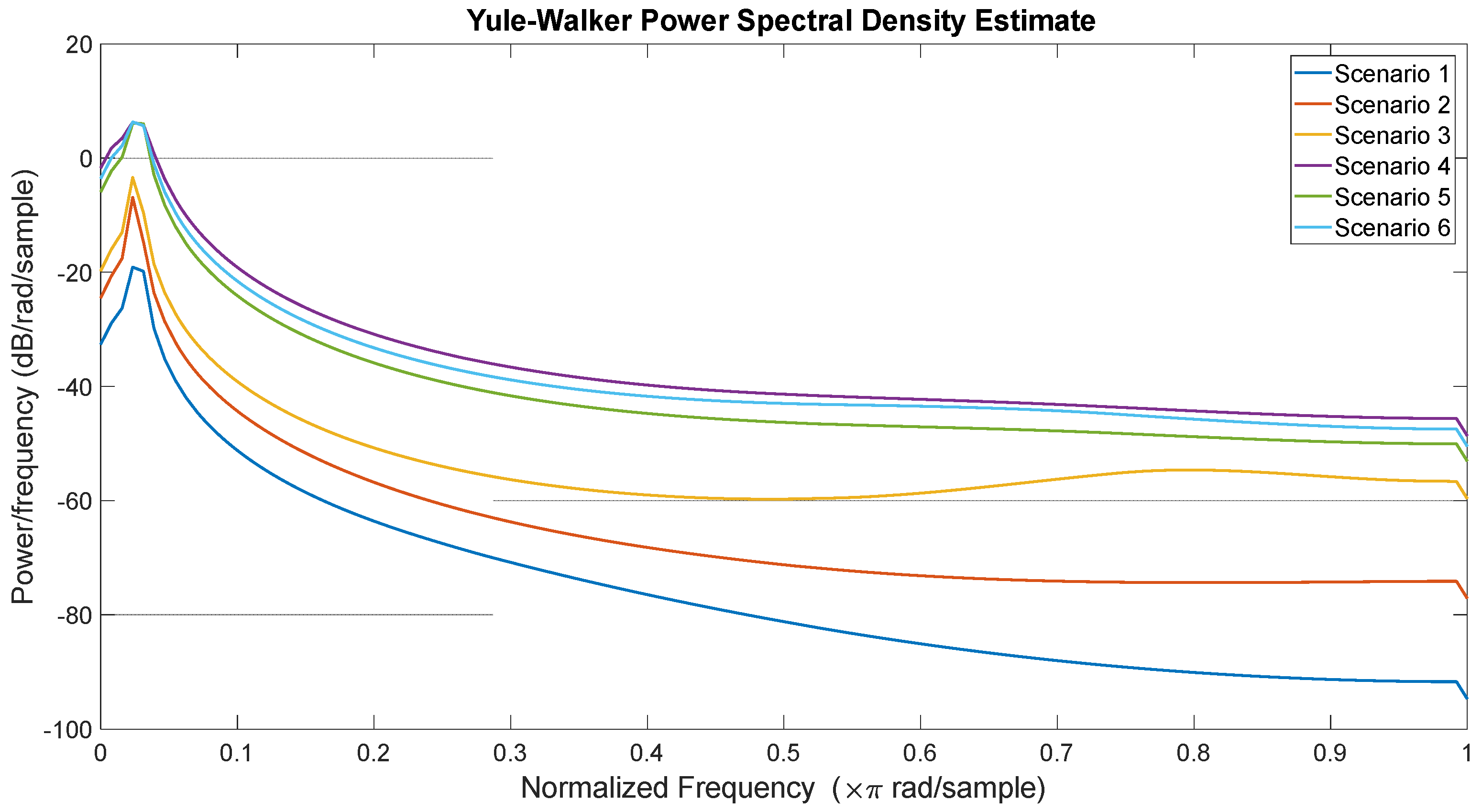
The AR coefficients () are obtained using the Levison–Durbin algorithm [53]. Figure 2 shows Yule–Walker Power Spectral Density (PSD) of all delamination levels in the WTB.
Akaike’s Information Criterion (AIC) has been used to reduce the dimensionality of the feature extraction. The AIC is a measure of the goodness-of-fit of an estimated statistical model, based on the trade-off between fitting accuracy and the number of estimated parameters. AIC is given by Equation (5):
where is the number of estimated parameters, the number of predicted data points, the error, and the average sum-of-square residual error.
3. Classification Procedure
3.1. Machine Learning Approach
A supervised classification is considered in ML, where the same number of signals is set for each group, or population. The cross-validation technique has been employed to estimate the probability of misclassification, and to avoid overfitting in all cases considered.
Decision Tree (DT) is a classifier used to determine if the dataset contains different classes of objects that can be interpreted significantly in the context of a substantive theory. DT generates a split of space from a labelled training set. The objective is to separate the elements of each class into different labelled regions, called leaves, minimizing a local error. Each internal node in the tree is a question, or decision, that determines the branch of the tree that must be taken to reach a leaf. DT is determined in the following cases: how to split the space, called Splitting Rules (SR); stopping the condition of splitting; labelling function of a region, and; measurement of error.
The purpose of the SR is to minimize the impurity of the node. In this case, SR is based on Gini’s Diversity Index (GDI) [54], given by Equation (7):
where the sum is over the classes i at the node, and p(i) is the observed fraction of classes with the class i that has the node. For a node with only one class, called the pure node, GDI = 0, being GDI > 0 in other cases. The algorithm stops if the node is pre-set at maximum depth; all elements of the node are the same class; there is no empty sub node; or SR does not reach a pre-set value.
DT labels a leaf, or region, when it is already considered as a terminal. The labelling function is set by Equation (8):
where is the number of elements of class l, is the class to label, and is the labelling cost.
The labelling cost considering all classes is calculated, and is selected to minimize the error, where a random one is chosen in case of a tie. Equation (9) provides a classification average error:
where is the error of labelling a class l as l’. This error will be solved by splitting the space and assigning a label to each split.
The number of partitions has been adjusted using the Decision Tree Complex (DTC) algorithm. It allows a maximum of 100 partitions to avoid overfitting.
Quadratic Discriminant Analysis (QDA) is employed to classify each feature (x) in pre-existing different groups, from the information of a set of variables (x), called variable classifiers [55]. The information of each variable (x) is synthesized in a discriminant function. Each class produces a dataset using Gaussian mixture distribution, given by Equation (10):
where and is the class k (k ≤ i ≤ K) population mean vector and covariance matrix.
The metric distance to each class is calculated using the variance–covariance matrix of each class, instead of the global matrix grouped in QDA [56], according to the Equation (11);
where is the squared distance between sample i, and the class k centroid, and is the corresponding variance–covariance matrix for that class.
The maximum of the a posteriori discriminant function , employing the Bayes rule and natural logs, is given by Equation (12):
K-Nearest Neighbors (KNN). The KNN classifier has been used for pattern classification and ML. The KNN is based on the principle that an unclassified instance within a dataset is assigned to the class of the nearest previously sorted instances [57]. Each instance can be considered as a point within an n-dimensional instance space, where each of the n-dimensions corresponds to one of the n-features that define an instance [58].
The accuracy of KNN classification depends on the metric used to compute distances between different instances. In this case, the best performing classifier is Weighted KNN (WKNN). WKNN assigns weights to neighbors regarding the distance calculated [59]. Weighted metric can be defined as a distance between an unclassified sample x, and a training sample , given by Equation (13):
3.2. Artificial Neuronal Network (ANN): Multilayer Perceptron (MLP)
In this paper, three layers of processing units are used as the structure (15/15/6). Backpropagation, together with the algorithm scaled conjugate gradient and performance cross entropy [60,61] with “early stopping” to avoid overfitting [62], has been employed as the training mode. ANN is given by Equation (14):
where . is the input, . the hidden layer output, . the final layer output, the target output, the hidden layer weight, . the final layer weight, hidden layer bias, the final layer bias, and (·) is the activation function sigmoid type.
The sigmoid function, Figure 3, is used as the activation function of the ANN, given by Equation (15). It provides an output in the range [0, 1].
The MLP is tested initially with an ANN architecture, and trained with 70% of the experiments. The ANN architecture is chosen according to the best accuracy and performance. The network is validated with different cases (30%) to determine if the learning is correct, and to check if it classifies correctly.
3.2.1. Training Process
Backpropagation (BP) is one of the simplest and most general methods for supervised training of multilayer ANNs. Techniques, such as scaled, have been developed to accelerate the training method BP, standardization, or normalization that performs pre-processing inputs. In this paper, BP mode algorithms are the scaled conjugate gradient and performance cross entropy.
Conjugate gradient algorithm, based on performing gradient descendent, is a second-order analysis of the error, employed to determine the optimal rate of learning, and extract information provided by the second derivative of the error by the Hessian matrix, (H), Equation (16).
The algorithm uses different approaches to avoid high computational costs. The MLP is employed in different stages during the learning process, where the reduction of error can be slow. It is suggested that the Mean Square Error (MSE) replaces the cross-entropy error function, because MSE shows a better network performance.
3.2.2. Architecture of the Network
Different ANN structures have been tested, and the structure that provides the best results was a hidden layer with 15 neurons, based on comparative performance by trial and error. The network architecture set was 15-15-6 (Figure 4).
3.3. Classifier Evaluation
The Receiver Operating Characteristic (ROC) analysis, based on Confusion Matrix (CM), is used to evaluate the classification. CM determines the quality of a classifier and its performance. The main parameters considered in CM are:
- TP: True positive is the real success of the classifier.
- FP: False positive is the sum of the values of a class in the corresponding CM column, excluding the TP.
- FN: False negative is the sum of the values of a class in the corresponding CM row, excluding the TP.
- TN: True negative is the sum of all columns and rows, excluding the column and row of the class.
The following equations will be applied to find the main measurement parameters when they are known:
- Recall, R, known as true positive rate, is the probability of being correctly classified, given by Equation (17).
- Specificity, S, also called the true negative rate, measures the proportion of negatives that are correctly identified, given by Equation (18).
Additional terms associated with ROC curves and CM are:
- Precision, P,
- F-score, F,
The average performance in all categories is set by two conventional methods [63]:
- Macro average (): , , is obtained by the averaging overall , where M denotes macro average, and i is the scenario. They are calculated for each category, i.e., the values precision is evaluated locally, , and then globally, .
- Micro average (): , and value is obtained as: (i) TPi, FPi, FNi values are calculated for each of the scenarios; (ii) the value of TP, FP, and FN are calculated as the sum of TPi, FPi, FNi; and (iii) applying the equation of the measure that corresponds to it.
There are several indices that are extracted from the ROC curve to evaluate the efficiency of a classifier. The Area Under Curve (AUC), value between 0.5 and 1, is the area between the ROC curve and the negative diagonal [64,65]. AUC ≤ 0.5 indicates that the classifier is invalid, and AUC = 1 indicates a perfect rating, because there is a region in which, for any point cut, the value of R and P is 1. The statistical property of AUC is equivalent to the Wilcoxon test of ranks [65]. The AUC is also closely related to the Gini coefficient [54], which is twice the area between the diagonal and the ROC curve.
The recommendations by Demšar, and Garcia and Herrera have been used to compare the different classifiers and analyze their best performance. Firstly, the Friedman Test will be used to test the null hypothesis that all classifiers achieve the same average. The Bonferroni–Dunn test will be applied to determine significant differences between the top-ranked classifier and the next one. The Holm test will be applied to contrast the results.
4. Case Study
The experiments were carried out in laboratory conditions. Regarding reference [66], it is possible to reproduce the test in working conditions by a multi frequency analysis. Low frequencies are associated with the vibration of the blade, medium frequencies with acoustic emissions, and high frequencies with the ultrasonic excitation signal.
Delamination, perpendicular to the direction of propagation according to Reference [19], has been carried out, with the smallest side perpendicular to the direction of propagation, and the larger side parallel to the propagation direction. The occurrence of multiple-delamination and transverse cracking has not been encountered in this study, but, according to [66], it would be affected in a similar way to the case study considered in this paper. Therefore, it would be possible to detect a potential failure with the presented approach.
Six different scenarios have been studied: the WTB without delamination (free of fault) was considered in the first scenario. A separation of layers was induced in the second scenario. The dimensions of the disunion were one centimeter wide by one centimeter deep. Subsequently, from scenarios three to six, deeper delamination was induced by increasing the depth in a centimeter in each state. Figure 5 shows the arrangement of the transducers and delamination in the WTB section, and Table 1 shows the deep values (x).
Guided waves were generated in the WTB section using Macro Fiber Composite (MFC) transducers. Figure 6 shows the transducer arrangement on the downwind side of the WTB. The ultrasonic technique used is called “pitch and catch” [67]. A short ultrasonic pulse is emitted by the MFC transmitter (Tx). The signal is collected by the MFC sensor (Rx). The excitation pulse is a six cycle Hanning pulse [68,69].
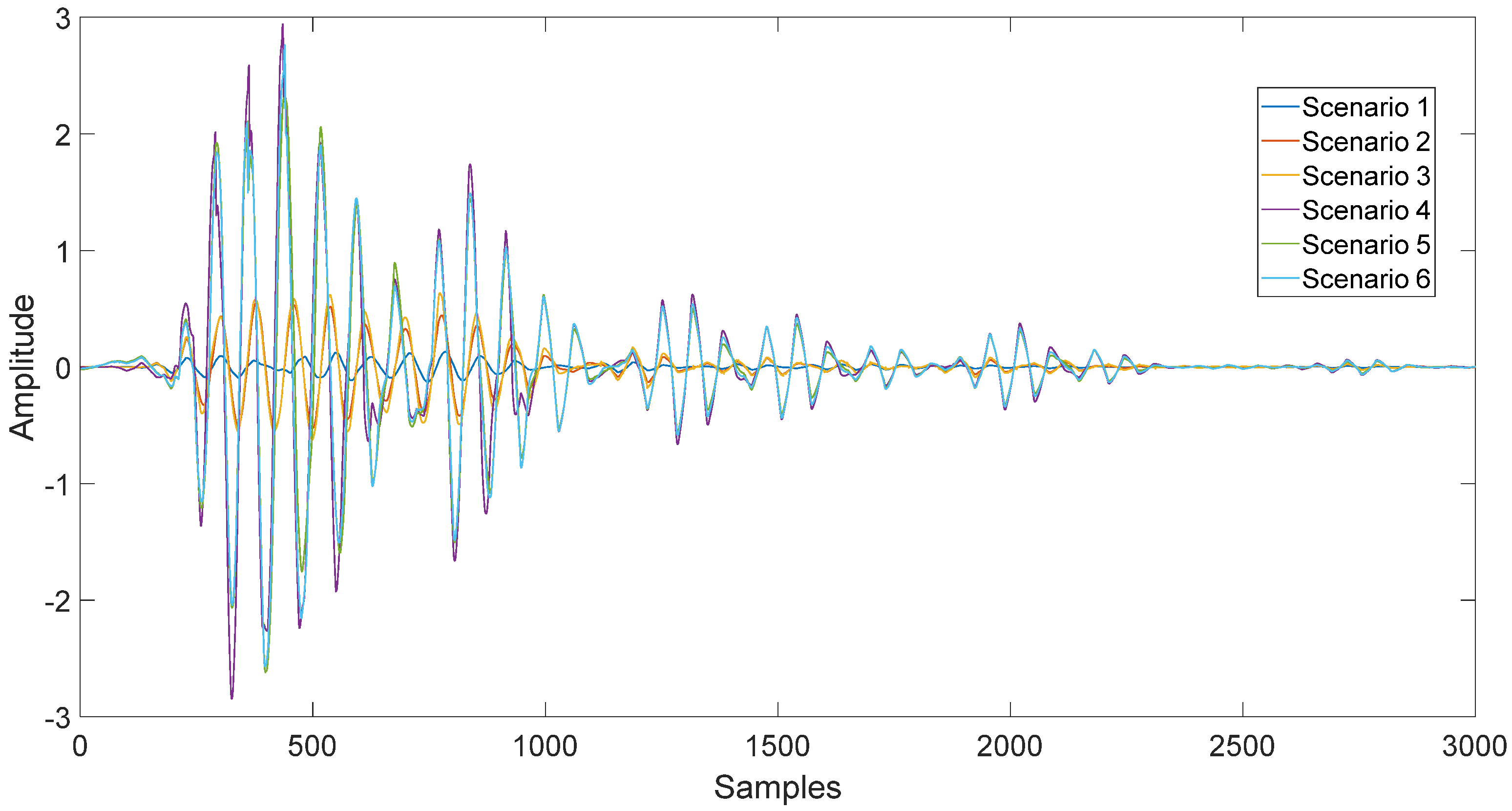
Five different excitation frequencies were conducted for each scenario of delamination to check the accuracy regarding the frequencies of delamination detection: 18 kHz, 25 kHz, 30 kHz, 37 Hz, and 55 kHz. Six hundred signals from each frequency were collected. The best accuracy was found at 55 kHz. Figure 7 shows signals acquired at 55 kHz in all scenarios.
5. Results and Discussion
5.1. Features Selection
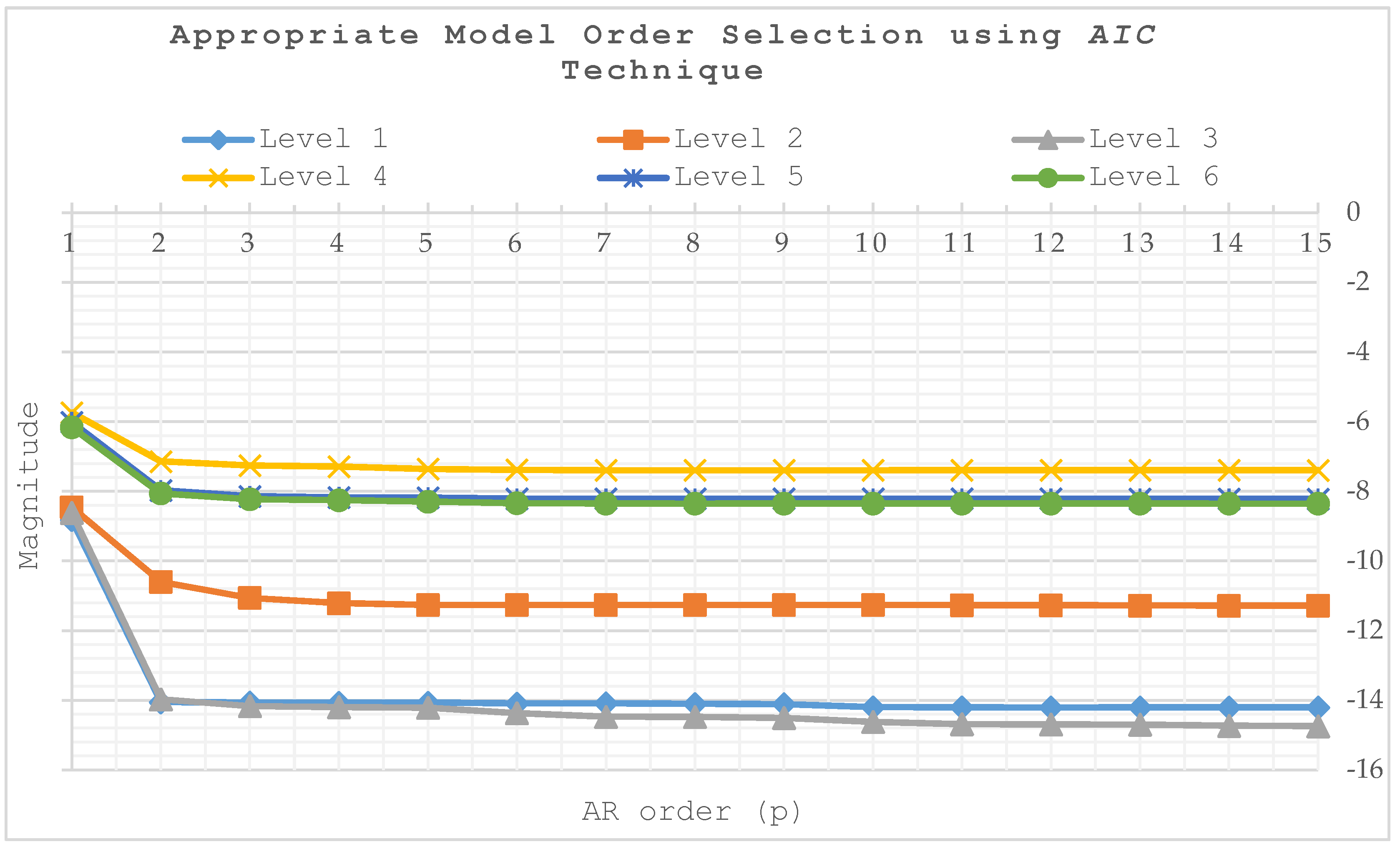
Fifteen features (the optimal range being from 15 to 30) have been used initially to avoid the problem of overfitting and over-dimensioning of the ANN architecture. The AIC method has been applied in all levels. In this case, the number of features that optimizes the model is p = 15 (see Figure 8) because the minimum AIC value for all levels is found. Therefore, the inputs were set to 15 for each classifier. The FPE criterion has been used, and produced similar results.
5.2. Precision
Table 2 shows that the lowest precision is for QDA classifier at Level 3, and is 28.50% in the worst case. The best case is found for WKNN at Level 5, 99.83%. Level 5 provides the best results in all classifiers. The results of micro average and macro average vary from 62.25% to 91.50%.
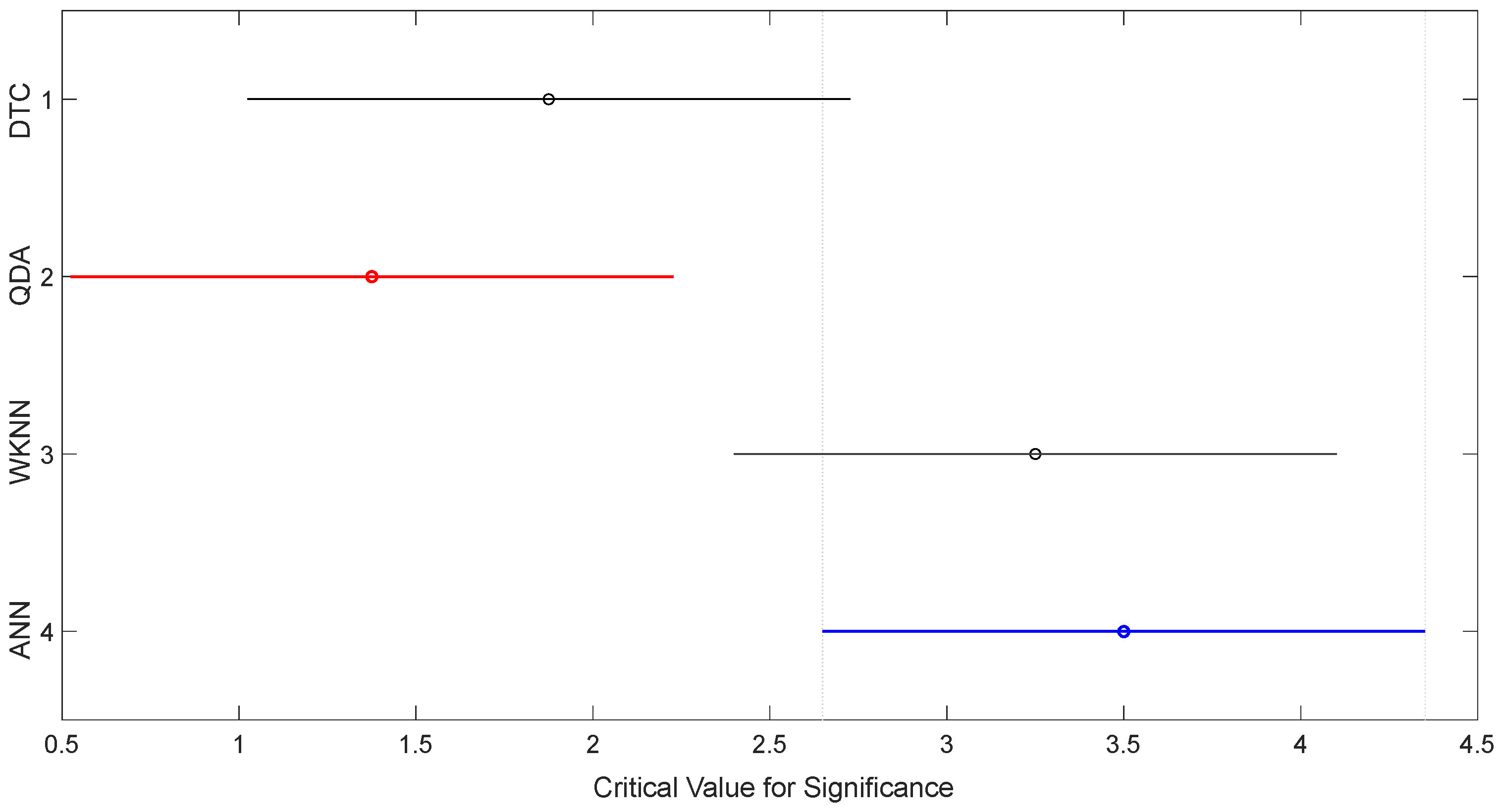
The recommendations by Demšar have been employed to analyze the results of the classifiers. The Friedman test E-1 did not reject the null hypothesis (p-value = 0.0169 ≤ 0.05). The Bonferroni–Dunn test rejected the null hypothesis for p ≤ 0.05, with a confidence value α = 0.05 (Figure 9). The Holm test rejected the null hypothesis for classifier 2.
The best accuracy was found by employing the ANN classifier (Table 2). The test indicates that QDA should be discarded.
5.3. Recall
The results are shown in Table 3. The Friedman test rejected the null hypothesis (p-value = 0.000076 ≤ 0.05), see Table 3. The rejection of the null hypothesis was confirmed by a post hoc test.
The Holm and Bonferroni–Dunn tests rejected the null hypothesis for the QDA classifier (Table 4).
5.4. F-score
The results given by F-score are shown in Table 5. The Friedman test rejected the null hypothesis (p-value = 0.000938 ≤ 0.05). The post hoc test showed that there is a significant difference between ANN and QDA classifiers. The Holm test provided the same results.
5.5. Area under Curve (AUC)
The Friedman, Holm, and post hoc tests rejected the QDA classifier (see Table 6). The classifiers WKNN and ANN showed the best results.
5.6. Discussion
The selection process is based on trial and error, and technical AIC for ANN. The optimal architecture of ANN is 15 input neurons, 15 hidden layer neurons, and 6 output neurons (number of levels).
ANN is the most accurate classifier with 91.50% success in real positives, where WKNN presents 90.97%. WKKN provides higher accuracy in 4 and 5 scenarios. ANN presents more sensitivity (91.50%).
F-score shows the best harmonic average of the precision and recall (91.50% for ANN and 90.98 for WKNN).
The AUC results are more than 0.91 for every level and ANN/WKNN.
QDA classifier was rejected. The Friedman, post hoc, Bonferroni–Dunn and Holm tests showed the existence of significant differences. In all cases, except for the QDA classifier, they indicated an accuracy rate of more than an 85% average, and 90% for the best classifier.
6. Conclusions
The main novelty presented in this paper has been to apply an approach for detecting and diagnosing the delamination in Wind Turbine Blades (WTB) to guided waves. The signals were experimentally obtained in a real WTB. The signal is filtered by wavelet transform with Daubechies family. The signal is studied by normalized and non-normalized signal tests, to avoid the effects of environmental and operational variations.
Feature extraction is done by the AR Yule–Walker model, and Feature Selection (FS) by Akaike’s information criterion.
The FS is done by the autoregressive model, where the selection process is based on trial and error, specifically for artificial neural network, where several input configurations and neuron nodes in the hidden layer have been tested.
Machine learning and artificial neuronal networks are used for pattern recognition. Six scenarios of delamination were considered. The approach detected and classified all the scenarios. The classifiers used to identify the scenarios are: quadratic discriminant analysis, k-nearest neighbors, and decision trees. The confusion matrix is used to evaluate the classification, especially the receiver operating characteristic analysis by recall, specificity, precision and F-score. The conventional methods to establish the average performance in all categories were macro and micro average. The recommendations by Demšar, and Garcia and Herrera have been used to compare the different classifiers and analyze their best performance. Firstly, the Friedman test has been used to confirm the null hypothesis that all classifiers achieve the same average. The Bonferroni–Dunn test has been applied to determine significant differences between the top-ranked classifier and the next one. The Holm test was applied to contrast the results. In this paper, the approach shows a high level of accuracy for the scenarios considered at room temperature, according to the results of the tests.
The performance of diagnostic system testing for multi-level detection of delamination in ANN and WKNN classifiers indicate a high level of accuracy, ANN being the best classifier.
Acknowledgments
The work reported herewith has been financially supported by the Spanish Ministerio de Economía y Competitividad, under Research Grants DPI2015-67264-P.
Author Contributions
The work presented here was carried out through the cooperation of all authors. A.A.J., C.Q.G.M. and F.P.G.M. conducted the research and wrote the paper. They edited the manuscript including the literature review. All authors read and approved the manuscript.
Conflicts of Interest
The authors declare no conflict of interest.
References
- García Márquez, F.P.; Pinar Pérez, J.M.; Pliego Marugán, A.; Papaelias, M. Identification of critical components of wind turbines using FTA over the time. Renew. Energy 2016, 87, 869–883. [Google Scholar] [CrossRef]
- Pliego Marugán, A.; García Márquez, F.P.; Pinar Pérez, J.M. Optimal maintenance management of offshore wind farms. Energies 2016, 9, 46. [Google Scholar] [CrossRef]
- Gómez Muñoz, C.Q.; García Márquez, F.P.; Tomás, J.M.S. Ice detection using thermal infrared radiometry on wind turbine blades. Measurement 2016, 93, 157–163. [Google Scholar] [CrossRef]
- Pinar Pérez, J.M.; García Márquez, F.P.; Hernández, D.R. Economic viability analysis for icing blades detection in wind turbines. J. Clean. Prod. 2016, 135, 1150–1160. [Google Scholar] [CrossRef]
- Pliego Marugán, A.; García Márquez, F.P.; Lev, B. Optimal decision-making via binary decision diagrams for investments under a risky environment. Int. J. Prod. Res. 2017, 1–16. [Google Scholar] [CrossRef]
- Pérez, M.A.; Gil, L.; Oller, S. Impact damage identification in composite laminates using vibration testing. Compos. Struct. 2014, 108, 267–276. [Google Scholar] [CrossRef]
- Pascoe, J.; Alderliesten, R.; Benedictus, R. Methods for the prediction of fatigue delamination growth in composites and adhesive bonds—A critical review. Eng. Fract. Mech. 2013, 112, 72–96. [Google Scholar] [CrossRef]
- Sohn, H.; Park, G.; Wait, J.R.; Limback, N.P.; Farrar, C.R. Wavelet-based active sensing for delamination detection in composite structures. Smart Mater. Struct. 2003, 13, 153. [Google Scholar] [CrossRef]
- McGugan, M.; Pereira, G.; Sørensen, B.F.; Toftegaard, H.; Branner, K. Damage tolerance and structural monitoring for wind turbine blades. Philos. Trans. R. Soc. A 2015, 373, 20140077. [Google Scholar] [CrossRef] [PubMed]
- García Márquez, F.P.; Pliego Marugán, A.; Pinar Pérez, J.M.; Hillmansen, S.; Papaelias, M. Optimal dynamic analysis of electrical/electronic components in wind turbines. Energies 2017, 10, 1111. [Google Scholar] [CrossRef]
- García Márquez, F.P.; Muñoz, J.M.C. A pattern recognition and data analysis method for maintenance management. Int. J. Syst. Sci. 2012, 43, 1014–1028. [Google Scholar] [CrossRef]
- García Márquez, F.P. A new method for maintenance management employing principal component analysis. Struct. Durab. Health Monit. 2010, 6, 89–99. [Google Scholar]
- Sohn, H.; Farrar, C.R.; Hunter, N.F.; Worden, K. Structural health monitoring using statistical pattern recognition techniques. J. Dyn. Syst. Meas. Control 2001, 123, 706–711. [Google Scholar] [CrossRef]
- Mellit, A.; Kalogirou, S.A. Artificial intelligence techniques for photovoltaic applications: A review. Prog. Energy Combust. Sci. 2008, 34, 574–632. [Google Scholar] [CrossRef]
- Ata, R. Artificial neural networks applications in wind energy systems: A review. Renew. Sustain. Energy Rev. 2015, 49, 534–562. [Google Scholar] [CrossRef]
- Bork, U.; Challis, R. Artificial neural networks applied to lamb wave testing of t-form adhered joints. In Proceedings of the Conference on the Inspection of Structural Composites, London, UK, 9–10 June 1994. [Google Scholar]
- Bork, U.; Challis, R. Non-destructive evaluation of the adhesive fillet size in a t-peel joint using ultrasonic lamb waves and a linear network for data discrimination. Meas. Sci. Technol. 1995, 6, 72. [Google Scholar] [CrossRef]
- Yam, L.; Yan, Y.; Jiang, J. Vibration-based damage detection for composite structures using wavelet transform and neural network identification. Compos. Struct. 2003, 60, 403–412. [Google Scholar] [CrossRef]
- Su, Z.; Ye, L.; Lu, Y. Guided lamb waves for identification of damage in composite structures: A review. J. Sound Vib. 2006, 295, 753–780. [Google Scholar] [CrossRef]
- Gomez Munoz, C.; De la Hermosa Gonzalez-Carrato, R.; Trapero Arenas, J.; Garcia Marquez, F. A novel approach to fault detection and diagnosis on wind turbines. Glob. NEST J. 2014, 16, 1029–1037. [Google Scholar]
- Gómez Muñoz, C.Q.; García Márquez, F.P. A new fault location approach for acoustic emission techniques in wind turbines. Energies 2016, 9, 40. [Google Scholar] [CrossRef]
- Rose, J.L. Recent advances in guided wave NDE. In Proceedings of the Ultrasonics Symposium, San Francisco, CA, USA, 16–18 October 1995; pp. 761–770. [Google Scholar]
- Rose, J.L. A baseline and vision of ultrasonic guided wave inspection potential. J. Press. Vessel Technol. 2002, 124, 273–282. [Google Scholar] [CrossRef]
- De da González-Carrato, R.R.; Márquez, G.; Pedro, F.; Papaelias, M. Vibration-based tools for the optimisation of large-scale industrial wind turbine devices. Int. J. Cond. Monit. 2016, 6, 33–37. [Google Scholar] [CrossRef]
- Worden, K.; Manson, G. The application of machine learning to structural health monitoring. Philos. Trans. R. Soc. Lond. A Math. Phys. Eng. Sci. 2007, 365, 515–537. [Google Scholar] [CrossRef] [PubMed]
- Jain, B.; Jain, S.; Nema, R. Investigations on power quality disturbances using discrete wavelet transform. Int. J. Electr. Electron Comput. Eng. 2013, 2, 47–53. [Google Scholar]
- Farrar, C.R.; Sohn, H.; Worden, K. Data Normalization: A Key for Structural Health Monitoring; Los Alamos National Lab.: Los Alamos, NM, USA, 2001.
- Gómez Muñoz, C.Q.; Jiménez, A.A.; García Márquez, F.P. Wavelet transforms and pattern recognition on ultrasonic guides waves for frozen surface state diagnosis. Renew. Energy 2017. [Google Scholar] [CrossRef]
- Gui, G.; Pan, H.; Lin, Z.; Li, Y.; Yuan, Z. Data-driven support vector machine with optimization techniques for structural health monitoring and damage detection. KSCE J. Civ. Eng. 2017, 21, 523–534. [Google Scholar] [CrossRef]
- Sharma, A.; Amarnath, M.; Kankar, P. Feature extraction and fault severity classification in ball bearings. J. Vib. Control 2016, 22, 176–192. [Google Scholar] [CrossRef]
- Manupati, V.; Anand, R.; Thakkar, J.; Benyoucef, L.; Garsia, F.P.; Tiwari, M. Adaptive production control system for a flexible manufacturing cell using support vector machine-based approach. Int. J. Adv. Manuf. Technol. 2013, 1–13. [Google Scholar] [CrossRef]
- Sohn, H.; Farrar, C.R. Damage diagnosis using time series analysis of vibration signals. Smart Mater. Struct. 2001, 10, 446. [Google Scholar] [CrossRef]
- Lu, Y.; Gao, F. A novel time-domain auto-regressive model for structural damage diagnosis. J. Sound Vib. 2005, 283, 1031–1049. [Google Scholar] [CrossRef]
- Yao, R.; Pakzad, S.N. Autoregressive statistical pattern recognition algorithms for damage detection in civil structures. Mech. Syst. Signal Process. 2012, 31, 355–368. [Google Scholar] [CrossRef]
- Nardi, D.; Lampani, L.; Pasquali, M.; Gaudenzi, P. Detection of low-velocity impact-induced delaminations in composite laminates using auto-regressive models. Compos. Struct. 2016, 151, 108–113. [Google Scholar] [CrossRef]
- Figueiredo, E.; Figueiras, J.; Park, G.; Farrar, C.R.; Worden, K. Influence of the autoregressive model order on damage detection. Comput. Aided Civ. Infrastruct. Eng. 2011, 26, 225–238. [Google Scholar] [CrossRef]
- Akaike, H. A new look at the statistical model identification. IEEE Trans. Autom. Control 1974, 19, 716–723. [Google Scholar] [CrossRef]
- Akaike, H. Fitting autoregressive models for prediction. Ann. Inst. Stat. Math. 1969, 21, 243–247. [Google Scholar] [CrossRef]
- Box, G.E.; Jenkins, G.M.; Reinsel, G.C.; Ljung, G.M. Time Series Analysis: Forecasting and Control; John Wiley & Sons: New York, NY, USA, 2015. [Google Scholar]
- Willmott, C.J.; Matsuura, K. Advantages of the mean absolute error (MAE) over the root mean square error (RMSE) in assessing average model performance. Clim. Res. 2005, 30, 79–82. [Google Scholar] [CrossRef]
- Konstantinides, K. Threshold bounds in SVD and a new iterative algorithm for order selection in ar models. IEEE Trans. Signal Process. 1991, 39, 1218–1221. [Google Scholar] [CrossRef]
- Mika, S.; Ratsch, G.; Weston, J.; Scholkopf, B.; Mullers, K.-R. Fisher discriminant analysis with kernels. In Proceedings of the Neural Networks for Signal Processing IX 1999, 1999 IEEE Signal Processing Society Workshop, Madison, WI, USA, 25 August 1999; pp. 41–48. [Google Scholar]
- Cunningham, P.; Delany, S.J. K-nearest neighbour classifiers. Mult. Classif. Syst. 2007, 34, 1–17. [Google Scholar]
- Quinlan, J.R. Induction of decision trees. Mach. Learn. 1986, 1, 81–106. [Google Scholar] [CrossRef]
- García Márquez, F.P.; García-Pardo, I.P. Principal component analysis applied to filtered signals for maintenance management. Qual. Reliab. Eng. Int. 2010, 26, 523–527. [Google Scholar] [CrossRef]
- De la Hermosa González, R.R.; García Márquez, F.P.; Dimlaye, V. Maintenance management of wind turbines structures via mfcs and wavelet transforms. Renew. Sustain. Energy Rev. 2015, 48, 472–482. [Google Scholar] [CrossRef]
- De la Hermosa González, R.R.; García Márquez, F.P.; Dimlaye, V.; Ruiz-Hernández, D. Pattern recognition by wavelet transforms using macro fibre composites transducers. Mech. Syst. Signal Process. 2014, 48, 339–350. [Google Scholar] [CrossRef]
- De Lautour, O.R.; Omenzetter, P. Damage classification and estimation in experimental structures using time series analysis and pattern recognition. Mech. Syst. Signal Process. 2010, 24, 1556–1569. [Google Scholar] [CrossRef]
- Daqrouq, K.; Abu-Isbeih, I.N.; Daoud, O.; Khalaf, E. An investigation of speech enhancement using wavelet filtering method. Int. J. Speech Technol. 2010, 13, 101–115. [Google Scholar] [CrossRef]
- Alfaouri, M.; Daqrouq, K. ECG signal denoising by wavelet transform thresholding. Am. J. Appl. Sci. 2008, 5, 276–281. [Google Scholar] [CrossRef]
- Birgé, L.; Massart, P. From model selection to adaptive estimation. In Festschrift for Lucien Le Cam; Springer: Berlin, Germany, 1997; pp. 55–87. [Google Scholar]
- Ramirez, I.S.; Gómez Muñoz, C.Q.; Marquez, F.P.G. A condition monitoring system for blades of wind turbine maintenance management. In Proceedings of the Tenth International Conference on Management Science and Engineering Management, Baku, Azerbaijan, 30 August–2 September 2016; pp. 3–11. [Google Scholar]
- Castiglioni, P. Levinson–durbin algorithm. In Encyclopedia of Biostatistics; John Wiley and Sons Ltd.: London, UK, 2005. [Google Scholar]
- Breiman, L.; Friedman, J.; Olshen, R.; Stone, C. Classification and Regression Trees; Wadsworth International Group: Belmont, CA, USA, 1984. [Google Scholar]
- Wu, W.; Mallet, Y.; Walczak, B.; Penninckx, W.; Massart, D.; Heuerding, S.; Erni, F. Comparison of regularized discriminant analysis linear discriminant analysis and quadratic discriminant analysis applied to NIR data. Anal. Chim. Acta 1996, 329, 257–265. [Google Scholar] [CrossRef]
- Friedman, J.H. Regularized discriminant analysis. J. Am. Stat. Assoc. 1989, 84, 165–175. [Google Scholar] [CrossRef]
- Cover, T.; Hart, P. Nearest neighbor pattern classification. IEEE Trans. Inf. Theory 1967, 13, 21–27. [Google Scholar] [CrossRef]
- Kotsiantis, S.B.; Zaharakis, I.; Pintelas, P. Supervised machine learning: A review of classification techniques. Inform. Int. J. Comput. Inform. 2007, 31, 249–268. [Google Scholar]
- Zuo, W.; Zhang, D.; Wang, K. On kernel difference-weighted k-nearest neighbor classification. Pattern Anal. Appl. 2008, 11, 247–257. [Google Scholar] [CrossRef]
- Møller, M.F. A scaled conjugate gradient algorithm for fast supervised learning. Neural Netw. 1993, 6, 525–533. [Google Scholar] [CrossRef]
- Kroese, D.P.; Rubinstein, R.Y.; Cohen, I.; Porotsky, S.; Taimre, T. Cross-entropy method. In Encyclopedia of Operations Research and Management Science; Springer: Berlin, Germany, 2013; pp. 326–333. [Google Scholar]
- Prechelt, L. Automatic early stopping using cross validation: Quantifying the criteria. Neural Netw. 1998, 11, 761–767. [Google Scholar] [CrossRef]
- Yang, Y. An evaluation of statistical approaches to text categorization. Inf. Retr. 1999, 1, 69–90. [Google Scholar] [CrossRef]
- Bradley, A.P. The use of the area under the ROC curve in the evaluation of machine learning algorithms. Pattern Recognit. 1997, 30, 1145–1159. [Google Scholar] [CrossRef] [Green Version]
- Hanley, J.A.; McNeil, B.J. The meaning and use of the area under a receiver operating characteristic (ROC) curve. Radiology 1982, 143, 29–36. [Google Scholar] [CrossRef] [PubMed]
- Gómez, C.Q.; Villegas, M.A.; García, F.P.; Pedregal, D.J. Big data and web intelligence for condition monitoring: A case study on wind turbines. In Handbook of Research on Trends and Future Directions in Big Data and Web Intelligence; IGI Global: Hershey, PA, USA, 2015; pp. 149–163. [Google Scholar]
- Gómez Muñoz, C.Q.; Arcos Jimenez, A.; García Marquez, F.P.; Kogia, M.; Cheng, L.; Mohimi, A.; Papaelias, M. Cracks and welds detection approach in solar receiver tubes employing electromagnetic acoustic transducers. Struct. Heal. Monit. 2017, 1475921717734501. [Google Scholar] [CrossRef]
- Gomez Munoz, C.Q.; Garcia Marquez, F.P.; Jimenez, A.A.; Cheng, L.; Kogia, M.; Mohimi, A.; Papaelias, M. A heuristic method for detecting and locating faults employing electromagnetic acoustic transducers. Eksploatacja I Niezawodnosc—Maint. Reliab. 2017, 19, 493–500. [Google Scholar] [CrossRef]
- Gómez Muñoz, C.Q.; García Marquez, F.P.; Lev, B.; Arcos, A. New pipe notch detection and location method for short distances employing ultrasonic guided waves. Acta Acust. United Acust. 2017, 103, 772–781. [Google Scholar] [CrossRef]
Figure 1.
Process for determining the level of delamination in the Wind Turbine Blades (WTB). Machine Learning (ML); Artificial Neural Networks (ANN).
Figure 1.
Process for determining the level of delamination in the Wind Turbine Blades (WTB). Machine Learning (ML); Artificial Neural Networks (ANN).
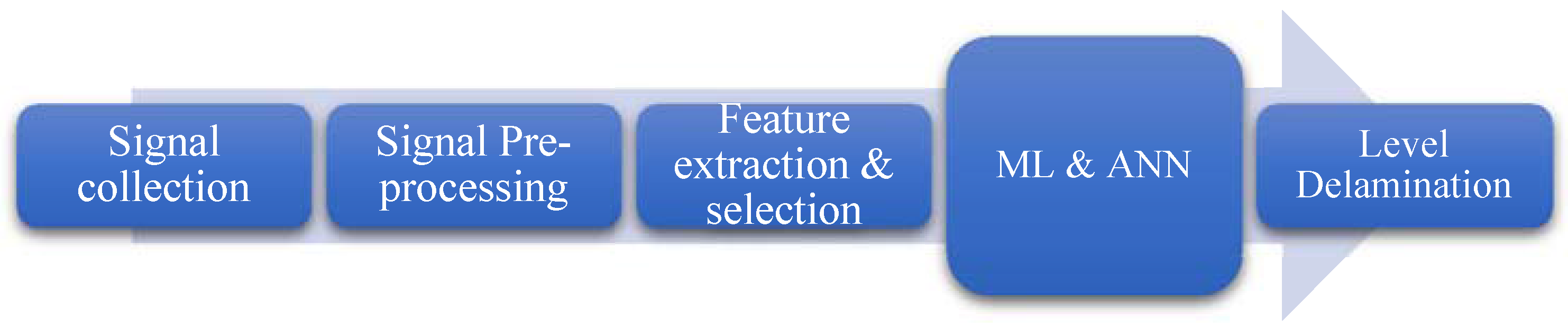
Figure 2.
Yule–Walker power spectral density for signals at 55 kHz in each scenario.

Figure 3.
Sigmoid activation function.
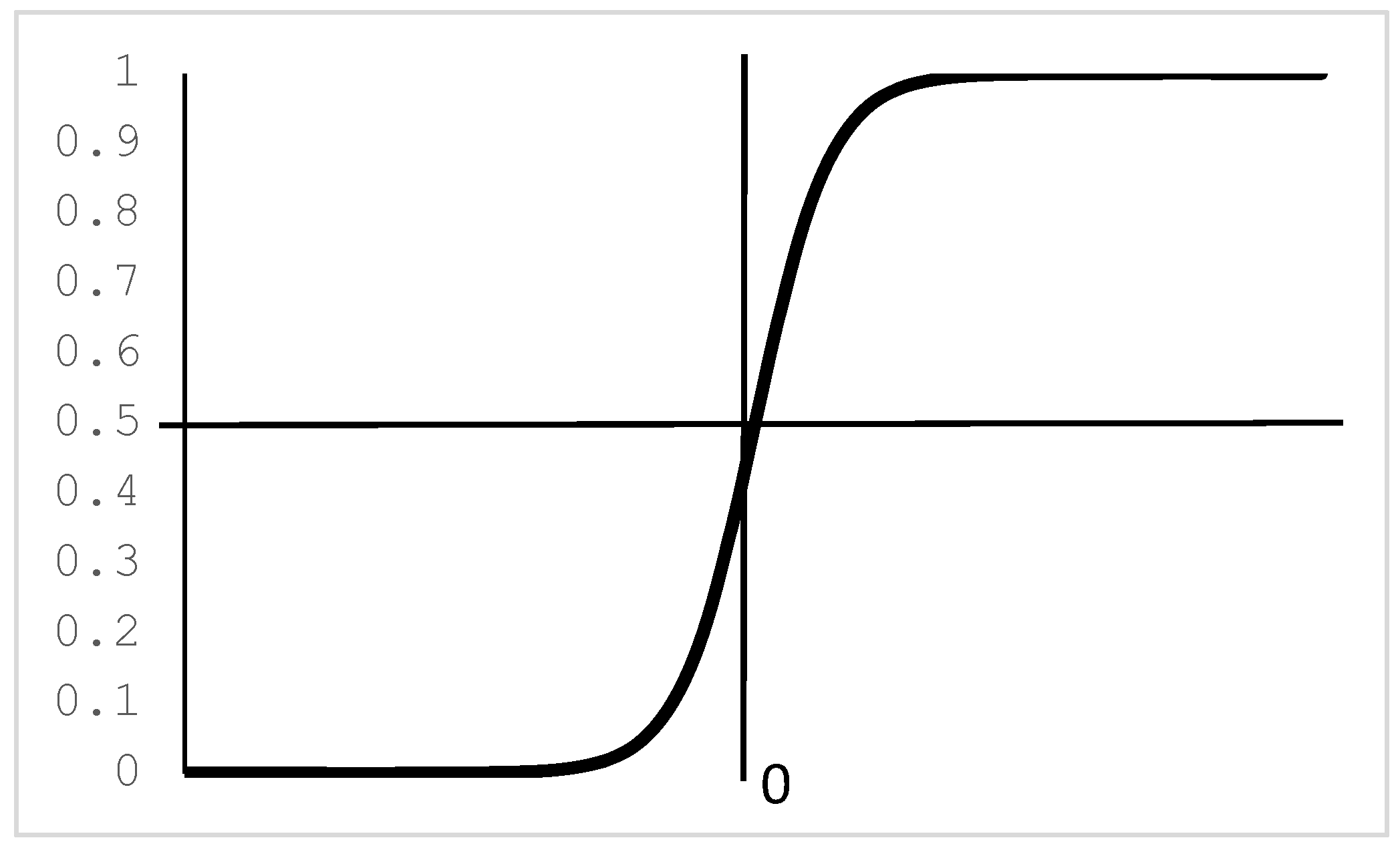
Figure 4.
Artificial Neural Networks (ANN) architecture.
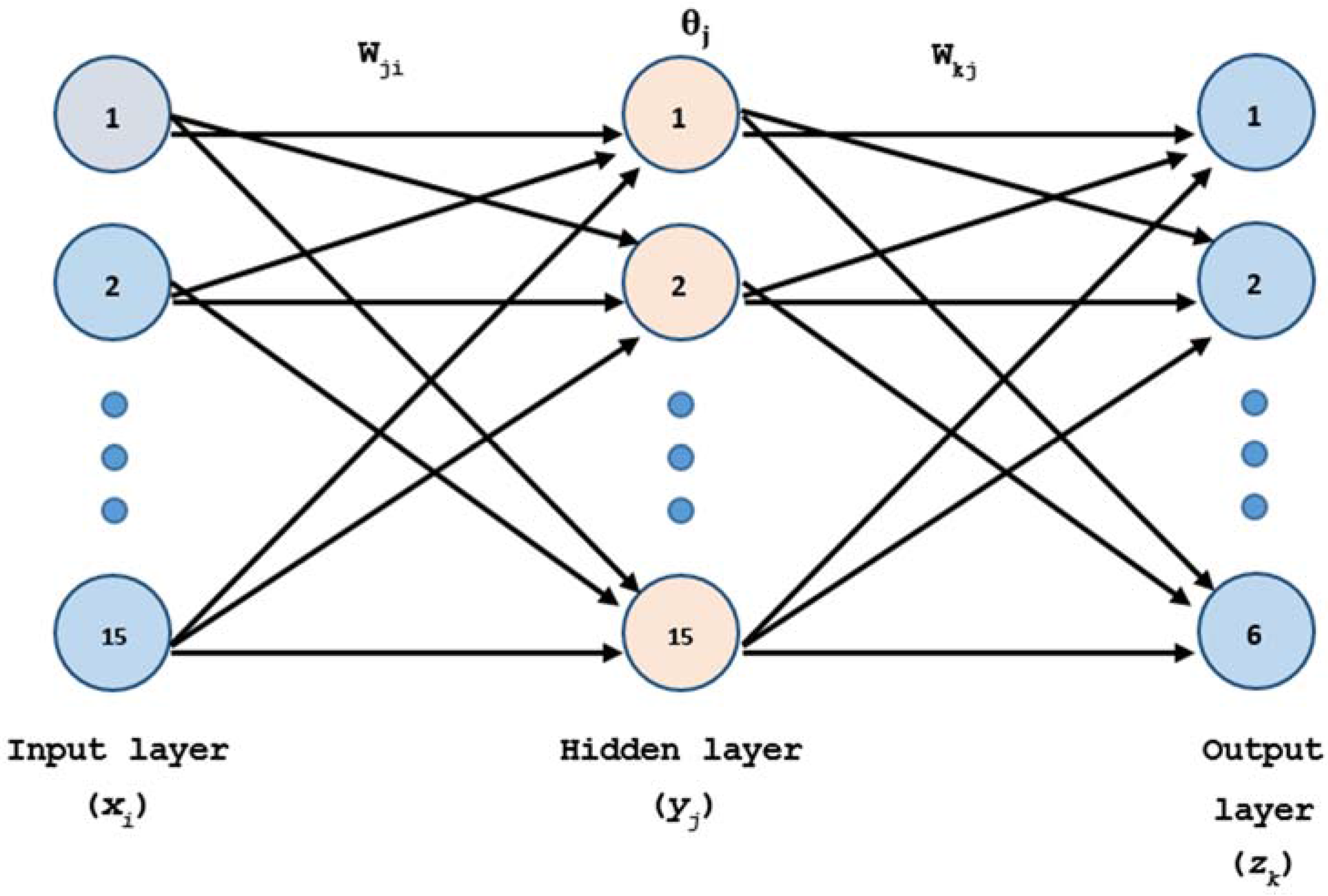
Figure 5.
Scheme of Macro Fiber Composite (MFC) transducers location for delamination detection.
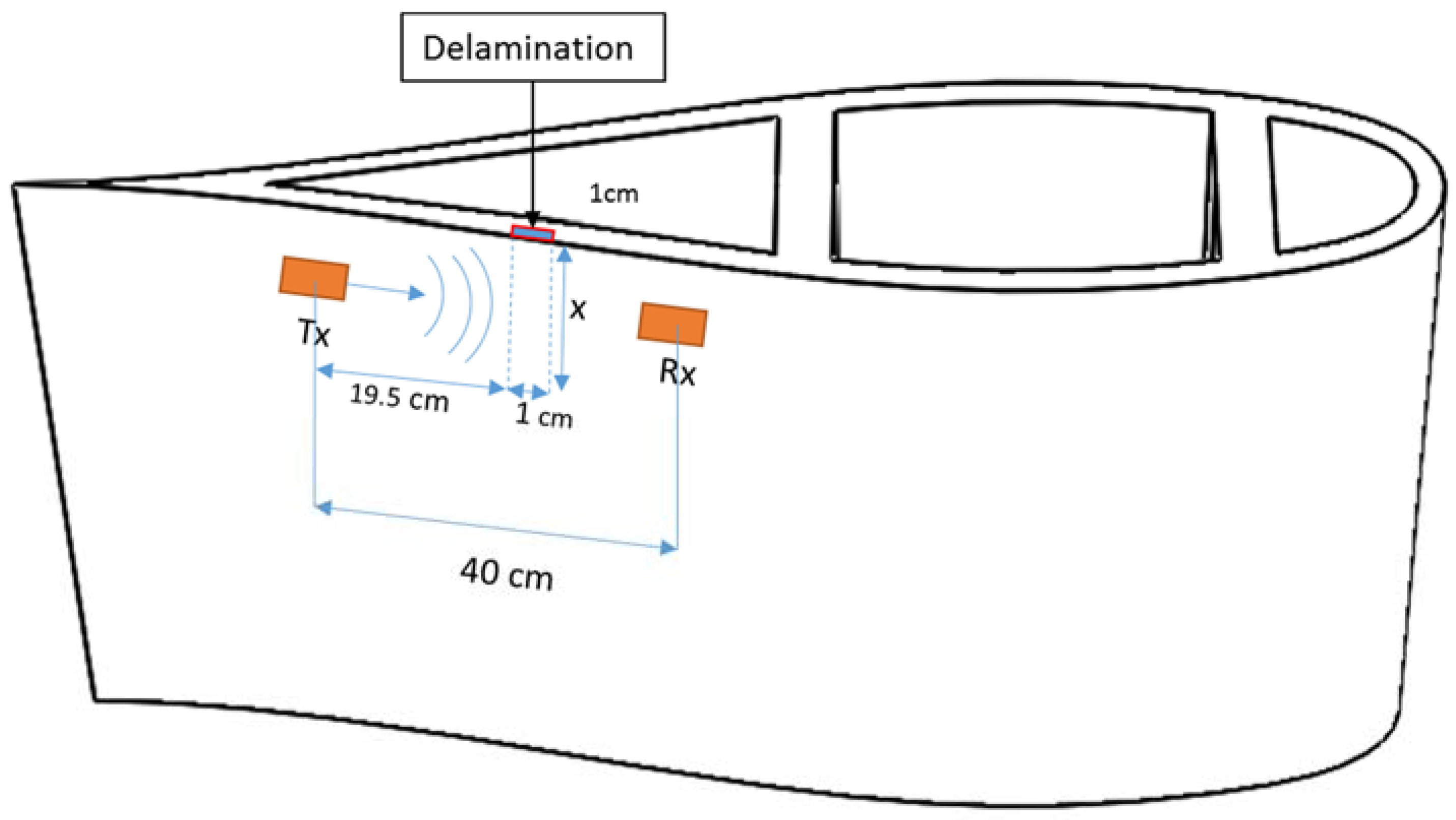
Figure 6.
Placement of sensor and delamination.
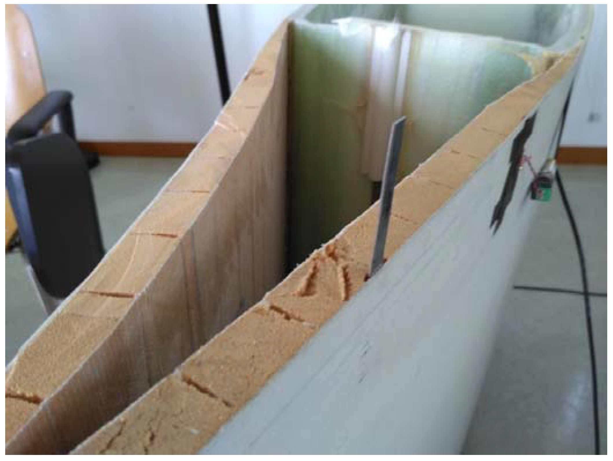
Figure 7.
Signals for different scenarios at 55 kHz.

Figure 8.
Akaike’s Information Criterion (AIC) curve features. AR: Auto-Regressive.

Figure 9.
Bonferroni-Dunn test. ANN: Artificial Neural Networks; WKNN: Weighted K-Nearest Neighbors; QDA: Quadratic Discriminant Analysis; DTC: Decision Tree Complex.
Figure 9.
Bonferroni-Dunn test. ANN: Artificial Neural Networks; WKNN: Weighted K-Nearest Neighbors; QDA: Quadratic Discriminant Analysis; DTC: Decision Tree Complex.

Table 1.
Delamination size in Wind Turbine Blades (WTB) section.
| Level | x (cm) | Delamination Area (cm2) |
|---|---|---|
| 1 | 0 (free of fault) | 0 |
| 2 | 1 | 1 |
| 3 | 2 | 2 |
| 4 | 3 | 3 |
| 5 | 4 | 4 |
| 6 | 5 | 5 |
Table 2.
Precision. DTC: Decision Tree Complex; QDA: Quadratic Discriminant Analysis; WKNN: Weighted K-Nearest Neighbors; ANN: Artificial Neural Networks.
Table 2.
Precision. DTC: Decision Tree Complex; QDA: Quadratic Discriminant Analysis; WKNN: Weighted K-Nearest Neighbors; ANN: Artificial Neural Networks.
| Level | DTC | QDA | WKNN | ANN |
|---|---|---|---|---|
| 1 | 0.8267 | 0.5633 | 0.8717 | 0.9262 |
| 2 | 0.8133 | 0.4000 | 0.8550 | 0.8583 |
| 3 | 0.7667 | 0.2850 | 0.8350 | 0.8593 |
| 4 | 0.9200 | 0.9217 | 0.9700 | 0.9089 |
| 5 | 0.9633 | 0.9733 | 0.9983 | 0.9934 |
| 6 | 0.8933 | 0.5917 | 0.9283 | 0.9457 |
| 0.8639 | 0.6225 | 0.9097 | 0.9150 | |
| 0.8639 | 0.6225 | 0.9097 | 0.9150 | |
| Ranking | 1.8700 | 1.3700 | 3.2500 | 3.5000 |
| Position | 3 | 4 | 2 | 1 |
Table 3.
Recall.
| Level | DTC | QDA | WKNN | ANN |
|---|---|---|---|---|
| 1 | 0.8656 | 0.7161 | 0.9175 | 0.9200 |
| 2 | 0.7428 | 0.5240 | 0.8328 | 0.8783 |
| 3 | 0.8028 | 0.3087 | 0.8254 | 0.8450 |
| 4 | 0.9200 | 0.7238 | 0.9417 | 0.9483 |
| 5 | 0.9666 | 0.6213 | 0.9788 | 0.9983 |
| 6 | 0.8948 | 0.8617 | 0.9653 | 0.9000 |
| 0.8639 | 0.6225 | 0.9097 | 0.9150 | |
| 0.8654 | 0.6259 | 0.9103 | 0.9150 | |
| Ranking | 2.0000 | 1.0000 | 3.1700 | 3.8300 |
| Position | 3 | 4 | 2 | 1 |
Table 4.
Test Holm.
| Test | p-Value | α | Comment |
|---|---|---|---|
| 2–4 | 0.0002 | 0.0085 | Reject Ho |
| 2–3 | 0.0003 | 0.0102 | Reject Ho |
| 1–2 | 0.0015 | 0.0127 | Reject Ho |
| 1–4 | 0.4551 | 0.0170 | Fail to Reject Ho |
| 1–3 | 0.4988 | No comparison made | Ho is accepted |
Table 5.
F-score.
| Level | DTC | QDA | WKNN | ANN |
|---|---|---|---|---|
| 1 | 0.8457 | 0.6306 | 0.8940 | 0.9231 |
| 2 | 0.7765 | 0.4537 | 0.8438 | 0.8682 |
| 3 | 0.7843 | 0.2964 | 0.8302 | 0.8521 |
| 4 | 0.9200 | 0.8109 | 0.9557 | 0.9282 |
| 5 | 0.9649 | 0.7584 | 0.9884 | 0.9958 |
| 6 | 0.8941 | 0.7016 | 0.9465 | 0.9223 |
| 0.8639 | 0.6225 | 0.9097 | 0.9150 | |
| 0.8642 | 0.6086 | 0.9098 | 0.9150 | |
| Ranking | 1.8300 | 1.5000 | 3.3300 | 3.3400 |
| Position | 3 | 4 | 2 | 1 |
Table 6.
Area under Curve (AUC).
| LEVEL | DTC | QDA | WKNN | ANN |
|---|---|---|---|---|
| 1 | 0.9170 | 0.8400 | 0.9480 | 0.9551 |
| 2 | 0.8760 | 0.7590 | 0.9070 | 0.9169 |
| 3 | 0.9030 | 0.6810 | 0.9020 | 0.9142 |
| 4 | 0.9520 | 0.8580 | 0.9680 | 0.9494 |
| 5 | 0.9890 | 0.8100 | 0.9890 | 0.9965 |
| 6 | 0.9510 | 0.9030 | 0.9760 | 0.9630 |
| Ranking | 2.4200 | 1.0000 | 3.0800 | 3.5000 |
| Position | 3 | 4 | 2 | 1 |
© 2017 by the authors. Licensee MDPI, Basel, Switzerland. This article is an open access article distributed under the terms and conditions of the Creative Commons Attribution (CC BY) license (http://creativecommons.org/licenses/by/4.0/).
Share and Cite
MDPI and ACS Style
Arcos Jiménez, A.; Gómez Muñoz, C.Q.; García Márquez, F.P. Machine Learning for Wind Turbine Blades Maintenance Management. Energies 2018, 11, 13. https://doi.org/10.3390/en11010013
AMA Style
Arcos Jiménez A, Gómez Muñoz CQ, García Márquez FP. Machine Learning for Wind Turbine Blades Maintenance Management. Energies. 2018; 11(1):13. https://doi.org/10.3390/en11010013
Chicago/Turabian StyleArcos Jiménez, Alfredo, Carlos Quiterio Gómez Muñoz, and Fausto Pedro García Márquez. 2018. "Machine Learning for Wind Turbine Blades Maintenance Management" Energies 11, no. 1: 13. https://doi.org/10.3390/en11010013
Note that from the first issue of 2016, this journal uses article numbers instead of page numbers. See further details here.