Informatics Solution for Energy Efficiency Improvement and Consumption Management of Householders


Department of Economic Informatics and Cybernetics, The Bucharest University of Economic Studies, Romana Square 6, Bucharest 010374, Romania
*
Author to whom correspondence should be addressed.
Energies 2018, 11(1), 138; https://doi.org/10.3390/en11010138
Submission received: 3 December 2017
/
Revised: 22 December 2017
/
Accepted: 1 January 2018
/
Published: 5 January 2018
(This article belongs to the Special Issue Selected Papers from SEEP2017: The 10th International Conference on Sustainable Energy and Environmental Protection)
Abstract
:Although in 2012 the European Union (EU) has promoted energy efficiency in order to ensure a gradual 20% reduction of energy consumption by 2020, its targets related to energy efficiency have increased and extended to new time horizons. Therefore, in 2016, a new proposal for 2030 of energy efficiency target of 30% has been agreed. However, during the last years, even if the electricity consumption by households decreased in the EU-28, the largest expansion was recorded in Romania. Taking into account that the projected consumption peak is increasing and energy consumption management for residential activities is an important measure for energy efficiency improvement since its ratio from total consumption can be around 25–30%, in this paper, we propose an informatics solution that assists both electricity suppliers/grid operators and consumers. It includes three models for electricity consumption optimization, profiles, clustering and forecast. By this solution, the daily operation of appliances can be optimized and scheduled to minimize the consumption peak and reduce the stress on the grid. For optimization purpose, we propose three algorithms for shifting the operation of the programmable appliances from peak to off-peak hours. This approach enables the supplier to apply attractive time-of-use tariffs due to the fact that by flattening the consumption peak, it becomes more predictable, and thus improves the strategies on the electricity markets. According to the results of the optimization process, we compare the proposed algorithms emphasizing the benefits. For building consumption profiles, we develop a clustering algorithm based on self-organizing maps. By running the algorithm for three scenarios, well-delimited profiles are obtained. As for the consumption forecast, highly accurate feedforward artificial neural networks algorithm with backpropagation is implemented. Finally, we test these algorithms using several datasets showing their performance and integrate them into a web-service informatics solution as a prototype.
1. Introduction
Energy efficiency targets, set by European Union (EU) leaders in 2007 and enacted in legislation in 2009, aim to reduce greenhouse gas emissions, improve energy security, and enhance competitiveness and sustainable development of entire society. The 2020 package is a set of binding legislations to ensure the EU meets its climate and energy targets for the year 2020. The EU has committed itself to energy and climate change objectives for 2020, comprising a 20% improvement in energy efficiency, higher share of renewable energy of 20% and reduction of greenhouse gas emissions by 20% compared with a baseline projection [1].
In 2012, the EU adopted Directive 2012/27/EU on energy efficiency that establishes a common framework of measures for the promotion of energy efficiency within the EU in order to ensure a 20% reduction of energy consumption by the year 2020. Then, in October 2014, EU countries agreed on a new energy efficiency target of at least 27% or greater by 2030. In November 2016, a new proposal for 2030 of binding energy efficiency target of 30% for the EU came up.
According to Eurostat, during the last ten years, although the households’ electricity consumption decreased by 1.3% in the EU-28, the largest expansions were recorded in Romania (48.1%), Lithuania (27.1%) and Spain (21.8%) which are among the EU members with higher electricity consumption [2].
Moreover, in Europe, the peak consumption is forecasted to increase by 38.77% in 2050 [3]; therefore, the growth rate is 1.1%. According to ENTSO-E, the annual monthly peak loads increase over the period 2016–2025 by 0.9%, although the energy consumption growth is slightly lower (0.8% annual) [4]. Also, in the US, the summer peak consumption is projected to increase by 1.5% yearly up to 2030, but at regional level, the growth rate is even higher [5]. However, the projected increase of the consumption peak will lead to additional onerous grid and generation capacity requirements that should be efficiently loaded only for short time periods; and higher electricity tariffs as a consequence of additional costs related to these capacities.
In the context of smart grids, by means of sensors, actuators, advanced tariffs, smart meters, IT and C infrastructure and other demand side management (DSM) measures, consumers become more and more active. Within rapid transition from traditional utility grid companies to smart micro-grids enhanced by significant growth of the sensors industry and communication facilities, the electricity consumers can categorize appliances into different types based on their shifting flexibility, model the day-ahead operation schedule of the appliances and agree to implement the optimized schedule that is related to a convenient time-of-use (ToU) tariff that reduces the electricity consumption payment. Usually, the micro-grid controller may identify customers with flexible loads which are willing to be controlled during critical periods in exchange for various incentives. However, promotion of energy efficiency, simulations and results estimation in terms of financial incentives regarding electricity payment and environmental benefits are vital for understanding the impact of consumption optimization strategies. The environmental benefits could be related to less number of km of transmission and distribution overhead lines and cables, increase of renewable distributed generation integration, etc.
Electricity consumption management brings significant benefits to consumers, prosumers, suppliers and grid operators. In terms of electricity consumption optimization, we show in [6] and [7] that planning of appliances operation brings savings to consumers and decrease the hourly demand peak. In [6], the optimum capacity of a storage device that significantly contributes to peak shaving of electricity consumption for residential consumers is calculated. It is based on the solution of two mixed integer linear programming (MILP) optimization problems: payment minimization and consumption peak minimization. Based on the results of [6], the best approach is to use storage devices to effectively contribute to the peak minimization and PV to obtain some savings.
In [8,9], the authors develop methods for load profile calculation using self-organizing maps (SOM) and applied classification or clustering in order to calculate accurate dynamic load profiles that could be used for electricity consumption forecast, market settlements and consumption optimization. Based on [8], the SOM are suitable for calculation of dynamic load profiles. Comparative analysis between [8] and [9] has shown that the best method for load profiles with specific patterns is clustering, while for well-delimited profiles, SOM is the most suitable method.
European Project Optimus aims to create a framework for assessing the local characteristics via the instrument OPTIMUS-SCEAF (Smart City Energy Assessment Framework) in the cities, develop a decision support system (DSS) to optimize energy use, implement it in three pilot European cities (Savona, Italy; San Cugat, Spain; and Zaanstac, The Netherlands) and make necessary training for expanding implementation of DSS [10].
Development of DSS for optimizing energy use by Optimus DSS has been initiated due to increased energy consumption in cities. They consume about two-thirds of the total consumption, are the largest sources of greenhouse gases and may affect about 70% of the total environmental footprint [11]. Optimus DSS is designed with the following modules: predictive module of consumption and production for renewable energy sources, statistics analysis module, consumers’ profiles module and consumption of electricity and heat optimization module.
In [12], the authors build IntelligEnSia solution (Intelligent Home for Energy Sustainability) that is focused on the prediction analytic using Web and Android technologies. For prediction of the energy consumption, the authors applied three regression models to predict the energy consumption based on the independent variable related to a particular day and dependent variables: current, voltage and power. The proposed models can support the decision-making process in obtaining energy consumption management.
In [13], the authors evaluate the impact of implementation of an energy management system. It is based on energy consumption and contributes towards sustainable development. The article performs an experimental design, using multiple linear regression to obtain a model that forecasts energy consumption.
In [14], the authors propose an optimal scheduling of hourly consumption at the community level based on real-time electricity tariff. The objective of the optimal load scheduling problem is to minimize the community electricity payment taking into account the consumption preferences of householders and characteristics of their appliances. Lagrangian relaxation is implemented to decouple the utility constraint and provide tractable sub-problems. The authors propose a multi-layer optimization approach. Starting from the initial case, first they considered adjustable and programmable appliances, then local generation, storage devices (in case they exist) and aggregated consumption of a certain micro-grid are involved. Therefore, gradually, the daily load flattens based on the real-time electricity tariff. The results show the efficiency of the proposed load scheduling method based on real-time electricity tariff.
Considering that existing demand side management strategies deal with only a limited number of controllable appliances of limited types, [15] proposes a DSM strategy based on load shifting technique for communities with large number of appliances in the smart grid context. The 24-h load shifting technique is a minimization problem that can be solved with a heuristic-based evolutionary algorithm. Simulations are performed considering three sectors: residential, commercial and industrial. The results show that the proposed DSM strategy brings significant savings, also reducing the peak load demand. However, the proposed load shifting technique may lead to the new peaks due to the fact that consumers would change the behavior and predominantly consume at the lower rate time intervals.
An interesting approach is given by [16] in which a methodology for ranking the EU funded energy efficiency projects with smarting interventions on the electricity grid is provided. It is based on ex-ante evaluation of the key performance indicators (KPIs) associated with environmental and energy-saving aspects, such as power savings, share of renewable energy sources and carbon emissions reduction. The methodology relies on optimal power flow algorithms, representing an appropriate tool for assessing the potential of projects that consist of smarting actions dedicated to accomplishing the 2020 EU targets.
In [17], the authors identify a high potential for savings and energy efficiency improvement of the residential sector in Spain and propose an energy planning methodology for evaluating the energy consumption of householders, primary energy consumption and share of renewable energy considering each energy source in a Spanish community (Riojan) and in Spain as a whole. The results provide KPIs at the residential sector level that show compliance with EU goals for 2020.
Paper [18] assesses the new-to-the-market climate change mitigation technologies that assist member states to reach EU 2020 goals. These technologies are aiming to achieving 20% of gross final energy consumption from renewables and achieving a 20% increase in energy efficiency. The paper provides an ex-post evaluation of the effectiveness of new-to-the-market climate change mitigation technologies.
Several questions on EU targets implementation pace and discrepancies in adoption of EU targets at the member states level are underlined by [19] in relation with achievement of a common development goal regardless of the significant differences in member states economy. The authors evaluate the implementation of the EU 2020 targets within the member states for years: 2004, 2010 and 2015. Based on this assessment, the member states are ranked according to the implementation stage. The proposed multidimensional approach allows comparison across member states in the evaluation years.
The scope of [20] consists of analyzing the possibilities of member states to fulfill the EU 2020 energy efficiency strategy and targets agreed in France (Paris). The authors show that rapid growth of economy and primary energy consumption generates more greenhouse gas emissions. However, their research reveals that the EU goal to reduce the greenhouse gas emission by 20% by 2020 compared with 1990 are achievable mainly by increasing the share of RES.
In [21], the author acknowledges that DSM including smart technologies and micro-generation at small to medium enterprises (SME) level plays an important role. The paper analyses the potential of smart technologies in SME from the United Kingdom, by developing a quantitative model to evaluate seven categories of smart technologies in ten non-domestic sectors. The results show that smart technologies provide important annual energy savings (17% savings on energy expenditures). The author also analyses the potential of micro-generation at the SME level searching for drivers and barriers to its implementation. It results that the initial costs, technical feasibility and planning permission on historical buildings are the main barriers, and that the feed-in tariffs is one of the main drivers.
Paper [22] analyses the energy demand of the residential sector; a comprehensive comparison is performed between control models (such as: thermostat, proportional-integral-derivative, model predictive control) of a domestic heating, ventilation and air conditioning system controlling the house temperature. As a novelty, the authors propose an interface that adjusts the model predictive control dynamic range of the output command signal into a discrete two level control signal. The analyzed house is also supplied by solar micro-generation, five ToU electricity rates being applied for a one week period. The aim of the proposed optimization approach is to reach the best compromise between temperature comfort and payment, identifying the most appropriate electricity rate option provided by the electricity supplier for the householders.
Paper [23] proposes an energy ecosystem, a cost-effective smart micro-grid based on intelligent hierarchical agents with dynamic demand response and distributed energy resource management. The individual costs of distributed energy resources and energy storage are, therefore, shared by the entire community. To achieve high energy efficiency in smart grids, the authors propose to shave the load by demand response, distributed energy resources and energy storage systems that can be optimally controlled.
In [24], the authors develop a couple of dynamic neural networks for solving nonlinear time series problems, based on the non-linear autoregressive and non-linear autoregressive with exogenous inputs models. Large datasets comprising the hourly energy consumption recorded by the smart meters installed at a commercial center type of consumer (hypermarket) and temperature and time stamp datasets (for non-linear autoregressive with exogenous inputs). As a novelty for consumption forecast, the authors obtain an optimal mix between the training algorithms Levenberg-Marquardt, Bayesian Regularization, Scaled Conjugate Gradient, the hidden number of neurons and the delay parameter.
Considering that savings achieved by the presence of smart metes are small, the authors of paper [25] analyze the potential of replacing the simple statement of energy use provided by an in-home displays with detailed information designed to improve consumer energy knowledge and recommend behavior change by personalized messages. The results point out the necessity of improving energy literacy in order to promote and encourage energy efficient measures and new smart meters with the potential to increase savings and impact climate change strategies.
Paper [26] proposes various DSM strategies using the genetic algorithm, teaching learning-based optimization, the enhanced differential evolution algorithm and the proposed enhanced differential teaching learning algorithm to manage energy and comfort, while taking the human preferences into consideration. The operation of programmable home appliances is changed in response to the real-time tariff signal in order to get monetary savings. To further improve the cost along with reduced carbon emission, renewable energy sources/energy storage are also integrated into the micro-grid. The main objectives are: RES integration, electricity bill reduction and minimizing the peak to average ratio and carbon emission. However, the objective of peak minimization should prevail due to its substantial advantages that lead to sustainable development of the power systems.
In [27], an overview and a taxonomy for DSM, analyzing the various types of DSM and giving an outlook on the latest demonstration projects in this domain are provided.
Energy efficiency services are expected to contribute to greenhouse gas emissions reduction and energy security at the EU level. Therefore, in [28], the authors carry out a case study and consider that the main challenges in developing new innovative energy efficiency services are: the unbundling of energy company activities, which makes it difficult to develop services when the contribution of several business units is necessary and the distrust among energy end-users, which renders the business logic of energy saving contract models self-contradictory.
In [29], the authors analyze the most relevant studies on optimization methods for DSM of residential consumers. They review the related literature according to three axes defining contrasting characteristics: DSM for individual users versus DSM for cooperative consumers, deterministic versus stochastic DSM and day-ahead versus real-time DSM. Thus, an image of the main features of different approaches and techniques is provided.
Paper [30] studies the general frame, software architecture, hardware platform and main modules of DSS for DSM. The system contains ten functions, including energy efficiency assessment, DSM program design, project management, electricity savings analysis, electric load analysis and forecast, peak load shifting management, policy modeling, project comprehensive evaluation, case management, that provide a complex decision supporting platform.
In [31], an energy retrofit intelligent DSS, that integrates expert knowledge with quantitative information to provide homeowners with accurate information for decision-making, is developed. The paper identifies the components of the proposed system, develops rules for relevant energy retrofit expert knowledge to be employed in the knowledge-based system of the DSS, develops the system for decision-making for home energy retrofits, and demonstrates the application of the DSS using two test homes. The paper contributes to improving the adoption of energy retrofits by homeowners.
In this paper, we propose a web-service integrated informatics solution that consists of three models for electricity consumption management that are based on optimization, profiles clustering and forecast algorithms developed in the smart grid context. Apart from other solutions, the input data is transformed and loaded into a relational cloud database and algorithms are implemented as stored procedures in the same database, increasing the performance of the processing algorithms, avoiding additional software tools for implementation.
To improve the energy efficiency, we propose to shift appliances to reduce the peak consumption and increase savings by avoiding onerous cost related to additional grid infrastructure. Moreover, by this solution, the consumers are able to monitor electricity consumption at the appliance level and identify the energy intensive appliances that can be replaced to reduce the electricity consumption and further increase the savings. Also, by our approach, the consumption profiles and forecast aim to increase the predictability of the consumption and improve the market strategies of suppliers that lead to electricity tariff reduction.
In the context of DSM, load control strategies for different purposes have to improve from conventional total load curtailments to shifting or adjusting the operation of appliances that does not affect or compromises the comfort of the consumers. However, by considering the consumption optimization problem only from the minimization of electricity payment point of view, as it is proposed in some research papers, it may generate new peaks as the consumers tend to shift their appliances to hours with lowest tariffs. Thus, our proposal is to shift the appliances in order to flatten the daily load curve as much as possible which will lead to the most convenient tariffs for consumers. In this respect, we design three algorithms that shift the programmable appliances, implement and compare the results.
Nevertheless, optimization strategies should be correlated with transparent and well-designed financial incentives and the intervention of consumers should be as light as possible, therefore, friendly online tools such as web portals are needed to reduce the consumers’ tasks [32]. Optimization algorithms help electricity suppliers to reshape the consumption profiles and obtain a more predictable forecast due to the optimal schedule operation at the appliance level. Also, the consumption optimization increases the awareness of consumers in terms of energy conservation and, thus, on medium and long-term consumption reduction.
For achieving consumption profiles, we develop a clustering algorithm based on self-organizing maps. By running the algorithm for three scenarios, different profiles are calculated. As a consequence, a comparative analysis section in the prototype to allow the supplier to visualize and compare the load profiles is designed.
As for the consumption forecast, feedforward artificial neural networks algorithm with backpropagation is implemented. Apart from consumption data, the dataset consists of exogenous factors such as: temperature, wind speed, wind direction, humidity, type of the day, hour and load profile. Then, the consumption management related algorithms are integrated into an informatics prototype that enables consumers and suppliers/grid operators to visualize data through interactive controls such as reports, pivot tables, charts, maps, scenarios and various gauges.
The paper is briefly structured as follows. Section 1 presents an introduction to the research work and different studies from literature. Section 2 describes the informatics solution for electricity consumption management components and architecture of the prototype. Section 3 shows the main flowchart for models and algorithms. Section 4 presents the proposed models and algorithms for consumption optimization, profiles and forecast. Section 5 shows the results. Section 6 depicts interfaces of the prototype. Section 7 presents discussion and Section 8 aims to provide the main conclusion remarks.
2. Informatics Solution for Electricity Consumption Management
Based on emerging technologies such as sensors, intelligent appliances, communications and smart metering systems, the advanced consumption management has been significantly enabled.
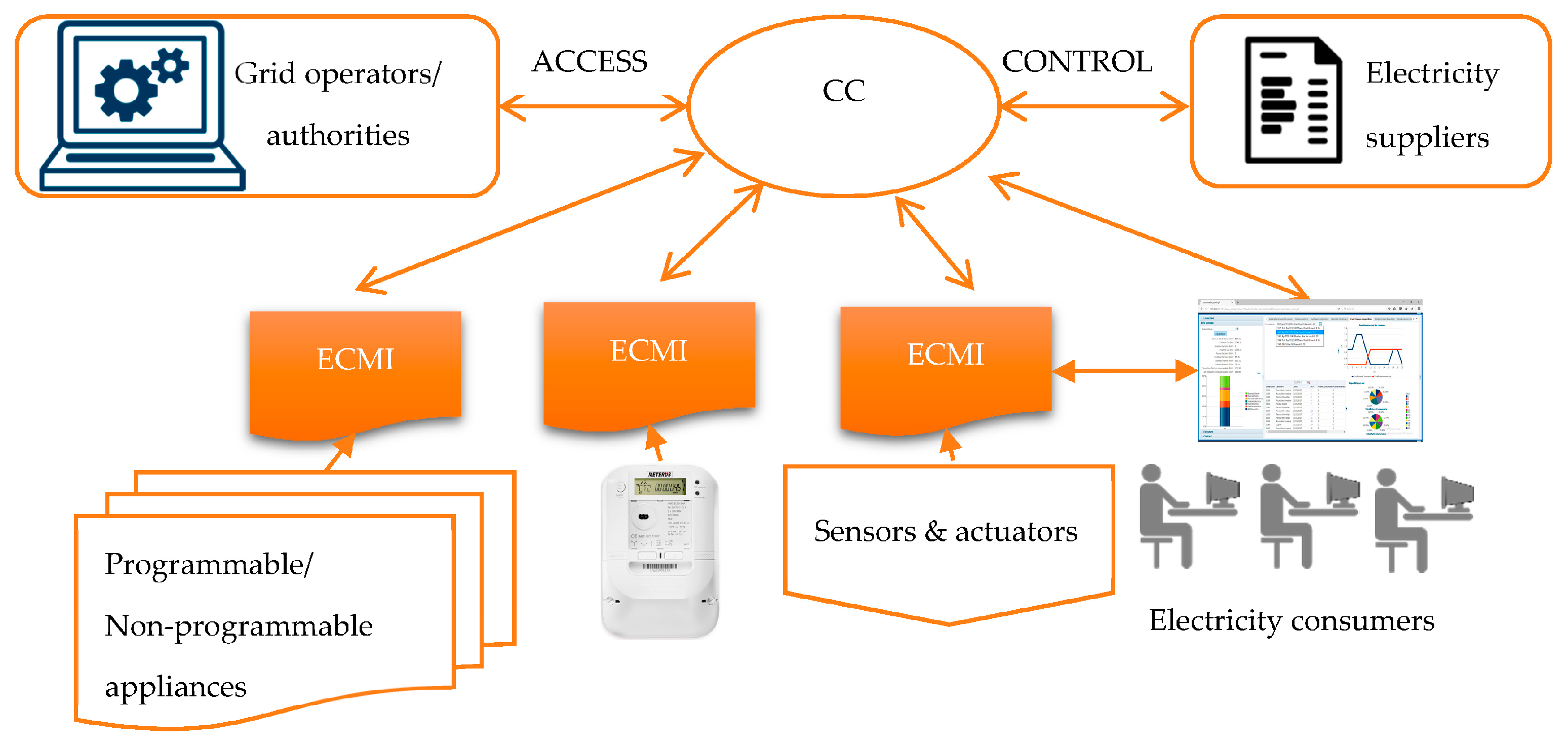
Nonetheless, the electricity consumption management mainly implies the interaction among users and components, such as electricity consumers need to control, schedule and monitor their appliances through a friendly user interface; electricity suppliers/grid operators require access to individual/aggregated consumption, profiles and forecast. Thus, our approach regarding consumption management consists of an informatics prototype developed on a cloud computing platform that integrates smart meters, programmable/non-programmable appliances and sensors through individual Electricity Consumption Management Instances (ECMI) and aggregates consumption at a Control Centre (CC) managed by the electricity supplier and accessed by the grid operators or other authorities (as in Figure 1).
The informatics prototype may assist decisions regarding consumption management, being developed as web-services accessible by three types of users: consumer has access to his appliances, consumption data, load scheduler, real-time bills, payments and tariffs through ECMI; electricity supplier has access to consumption data, load profiles, consumption forecast and can set up tariffs through CC; grid operator, authority and/or regulator may access CC to analyze the aggregated consumption data for grid or market related purposes.
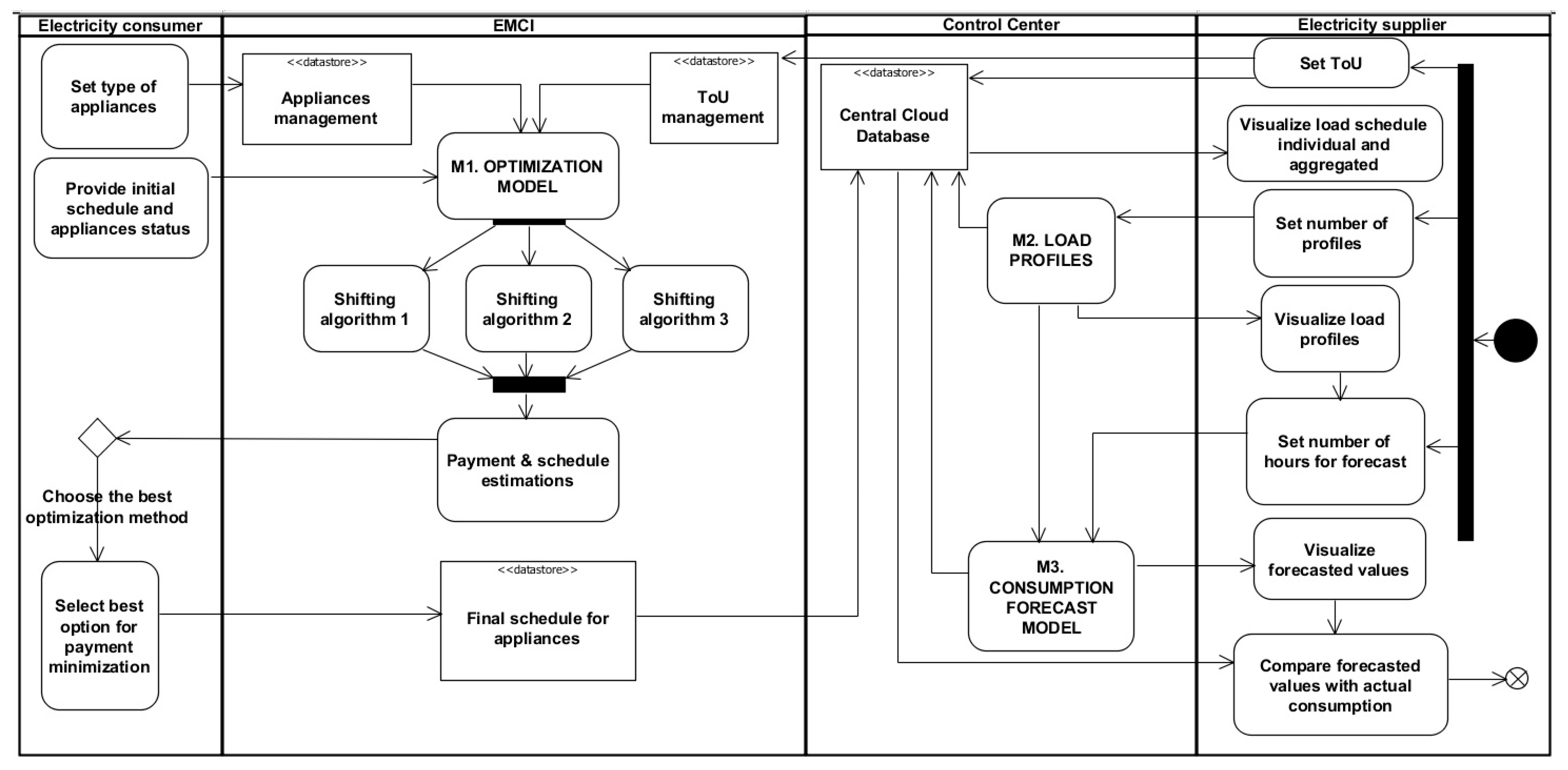
Architecture of the prototype is presented in Figure 2. Appliances and smart meters are connected within a network of sensors designed to control the operation of the appliances. The input data collected from individual appliances are loaded into a central database through a gateway. From the database, in order to enable advanced and multidimensional analyses, data is transformed and loaded into a data warehouse. Then, data is processed within three distinct models: M1, electricity consumption optimization; M2, load profiles; and M3, consumption forecast; for each model, specific algorithms are developed. Users interact with the proposed models via web-services, each type of user having access to specific options. Electricity consumers visualize their hourly consumption, real-time billing information, tariffs and have access to module M1. Also, through the interface, the consumer’s preferences and characteristics of electric appliances are added. Based on the consumers’ input regarding appliances and their preferences, the algorithms implemented in M1 optimize the hourly consumption, providing the optimal schedule of each appliance.
Individual consumption optimization of each consumer is performed at the ECMI level, the operation of the appliances is stored in the database and subsequently loaded into the data warehouse for historical advanced analyses. Consumption optimization process also considers the non-programmable appliances, such as: refrigerator, lighting, etc., but it is achieved mainly through programmable appliances, such as washing machine, bread oven, dryer, car battery, etc. After consumption optimization is performed, the ECMI sends to CC the planning (operation schedule) consumption for a certain period of time, usually 24 h. Based on the consumption data recorded at regular intervals of time (hour by hour or at 15 or 30 min), the consumption profiles (M2 model) are determined with clustering algorithm developed with SOM. For each profile, the electricity supplier performs consumption forecast with artificial neural networks (ANN) by accessing M3 model. Compared with the present situation, when hourly consumption is unknown, based on detailed data collected from consumers, the supplier and grid operator are able to analyze consumption and provide accurate consumption forecasts at the CC level, which have a positive impact on grid operation planning and actions on electricity wholesale market.
For consumption management purposes, we develop an online portal that allows advanced analyses for suppliers that include data visualization elements via dashboards, predictive analyses, what if scenarios, planning and reporting tools.
Also, the prototype includes interfaces for consumers to enable real-time information regarding consumption and tariff scheme visualization, consumption monitoring, alerts and consumption thresholds, comparisons between consumption within the same profile while preserving the data confidentiality, consumption estimations and predictions.
In Section 3, the flowchart of the models and algorithms is presented.
3. Flowchart of the Proposed Models and Algorithms
The proposed models and algorithms are integrated through the web-services in the main interface of an informatics prototype and allow the execution of the optimization algorithms performed by the consumers on one side and the execution of the load profile and consumption forecast algorithms performed by the electricity supplier on the other side. Users’ interaction with the proposed models and the algorithms is described in Table 1.
Flowchart of the models and algorithms in Figure 3 shows the connections between users (electricity consumers and supplier), the individual electricity consumption management instances (ECMI) and the control center (CC).
Optimization algorithms are executed in ECMI, while the load profiles and consumption forecast are executed in the control center (CC). All outputs provided by algorithms are stored in a central database for further analyses and historical records. Also, from the central database, electricity supplier can compare forecasting results with actual consumption to evaluate the accuracy of the algorithm. Both CC and ECMI are developed in a cloud computing platform and accessed via web-services.
In the Section 4, we describe the models M1, M2 and M3 developed and integrated into the prototype. These models are tested in Section 5 on hourly consumption dataset for 212 consumers during one year period. Data is collected from smart meters and sensors for several types of appliances: heating, cooling, ventilators, indoor lighting, outdoor lighting, water heating, household equipment (washing machine, refrigerator and coffee maker) and other interior devices (TV, PC, sound systems). For consumption forecast model, data is collected also from weather sensors (temperature, humidity, wind speed, wind direction). The data is checked for consistency and measurements are validated and loaded into the central database running Oracle Database 12c, where the proposed algorithms are implemented as stored procedures in Oracle PLSQL language.
4. Models and Algorithms
4.1. M1—Optimization Model. Algorithms for Shifting the Householder Programmable Appliances
The operation of programmable appliances can be shifted to flatten the consumption peak by means of ToU or real-time tariffs that are designed to support such objective. As a consequence, the suppliers are able to offer attractive ToU tariffs if the consumption is more predictable and can improve the strategies on the electricity markets.
In this respect, we develop three algorithms that aim to shift the operation of programmable appliances in order to reduce the consumption peak as much as possible. The consumers have only to define the type of their appliances and send the operation schedule (hourly consumption preferences) that will be optimized by ECMI, so that convenient ToU tariff is applied for electricity consumption.
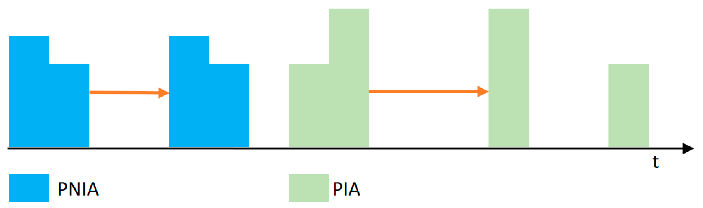
For implementation, we consider several appliances with fixed operation schedule (also known as non-programmable appliances or NPA), such as: refrigerator, electric oven, etc. that cannot be shifted due to consumers’ comfort reasons. From this category, some appliances that are always in operation are also known as background appliances [33] (such as refrigerator, house monitoring system). Then, we consider programmable with interruption appliances or programmable with interruption appliances (PIA) (i.e., car battery, water heater, vacuum, heating system, etc.) and programmable non-interruptible appliances or programmable non-interruptible appliances (PNIA) (i.e., washing machine, bread oven, dish washer, etc.). For privacy reasons, consumers can only mention the type of the appliances (non-programmable appliances (NPA), PIA or PNIA) without disclosing private information regarding consumption activities and brand of appliances.
The shifting flexibility of these appliances is depicted in Figure 4. PNIA will shift with entire hourly consumption blocks, while PIA will shift block by block since they support interruptions in operation.
For optimizing the operation of the appliances, the consumer should provide only the day-ahead desirable schedule for all appliances based on their type and status matrix (S—the possible operation time interval, where 1 is on and 0 is off) of the programmable appliances. For programmable appliances, it is important to know the possible operational time intervals that indicate the availability of either appliance or consumer. Based on them, the possible starting time can be figured out taking into account the operation duration.
The shifting algorithms are iterative processes that consider non-programmable appliances as fixed hourly consumption and programmable appliances aiming to flatten the daily load curve taking into account the operation constraints of programmable appliances. The operation constraints are related to the possible operation hours for a certain appliance. For instance, some appliances cannot operate without consumers’ intervention (also known as active appliances) such as vacuum, while some appliances have to be at home in order to consume (e.g., car battery, also considered as passive appliances) [33].
Consumption shifting of the appliances takes advantage of time independence of loads and follows the filling valley technique, but sometimes there are dependencies among appliances operation. For instance, the dryer will operate always after washing machine finished its operation. So, additional constraints has to be considered.
The actual optimized consumption for hour h after shifting the appliances is equal with the total scheduled consumption of all appliances, , plus total consumption of shifted appliances to hour h plus total consumption of shifted appliances to hour h d, , minus total consumption of shifted appliances i from hour h minus total consumption of shifted appliances j from hour h , .
where:
- N—total number of appliances;
- —actual consumption at hour h;
- —scheduled consumption of appliance q at hour h;
- —consumption of shifted appliance to hour plus consumption of shifted appliance to hour ;
- —consumption of shifted appliance from hour plus consumption of shifted appliance from hour h ;
- d—time interval before and after hour h that is required by PNIA appliances to operate.
When shifting a programmable interruptible appliance (PIA), the total consumption for peak and off-peak hours becomes:
where:
- —total consumption at off-peak hour;
- —total consumption at peak hour with at least one programmable appliance that can be shifted;
- —consumption of programmable appliance that shifts from peak to off-peak hour;
It means that the off-peak consumption increases by the shifted consumption of PIA, while the peak consumption decreases by the same amount.
For PIA, there is no need to calculate the operation duration since its operation can be interrupted.
If shifting a programmable non-interruptible appliance (PNIA), first we need to identify the start and end operation hours of the appliance and calculate its operation duration:
where:
- —operation duration for PNIA;
- —start and end operation hours at peak;
Then, the shifting algorithm verifies the possible starting hours (status matrix S) around off-peak hour proximity to find (start operation hour at off-peak) and accordingly shifts the appliance. Starting from to and to , then:
Also, the consumption in the proximity of the peak hour will decrease due to the fact that PNIA may start/end operation before or after the peak hour.
In all proposed algorithms, the appliances are shifted until the total consumption at peak hour with at least one programmable appliance that can be shifted ( is smaller or equal to the average consumption and the total off-peak consumption plus shifted consumption is greater or equal to the total peak consumption that has programmable appliances that can be moved.
where represents the average hourly consumption.
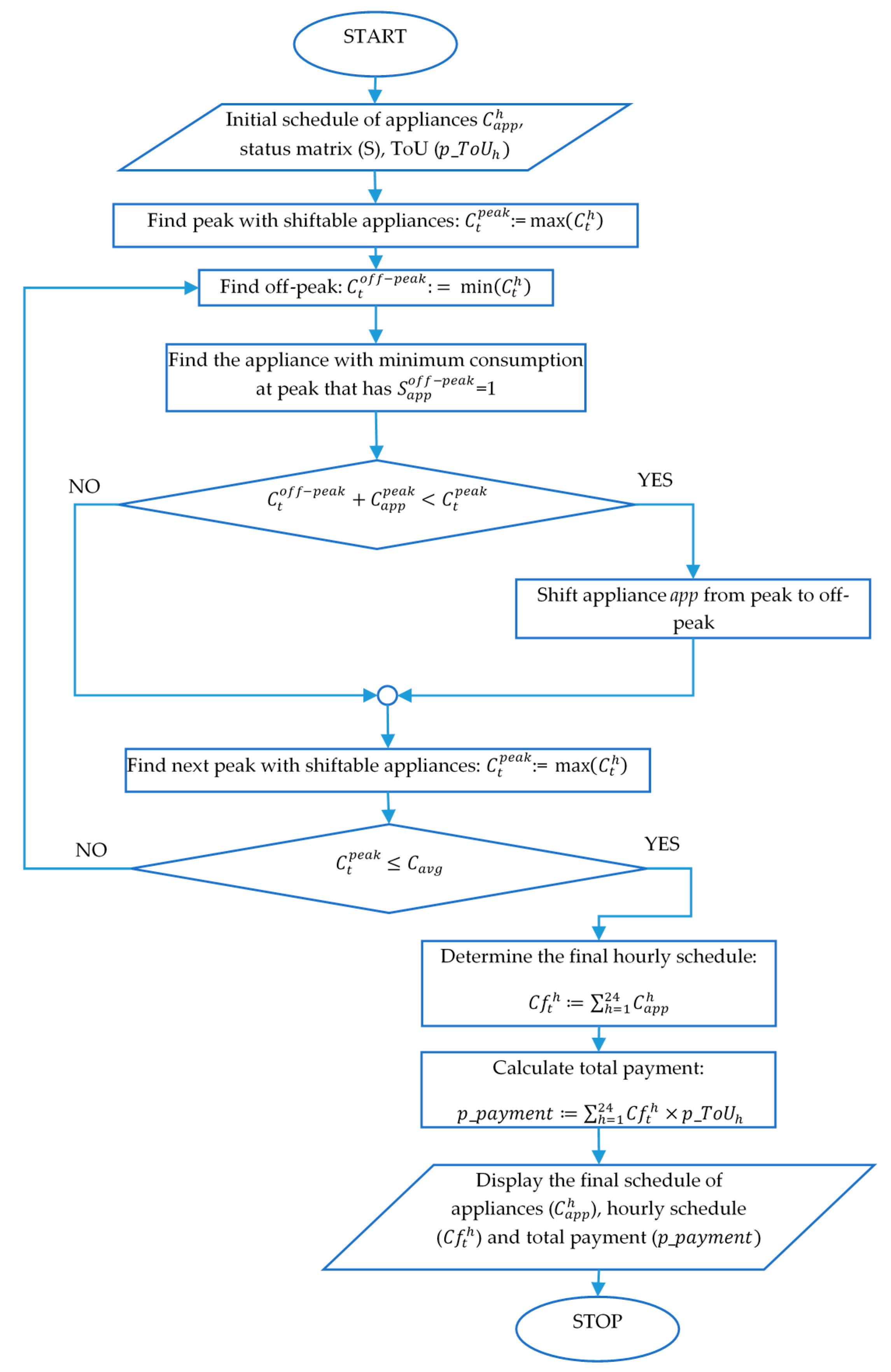
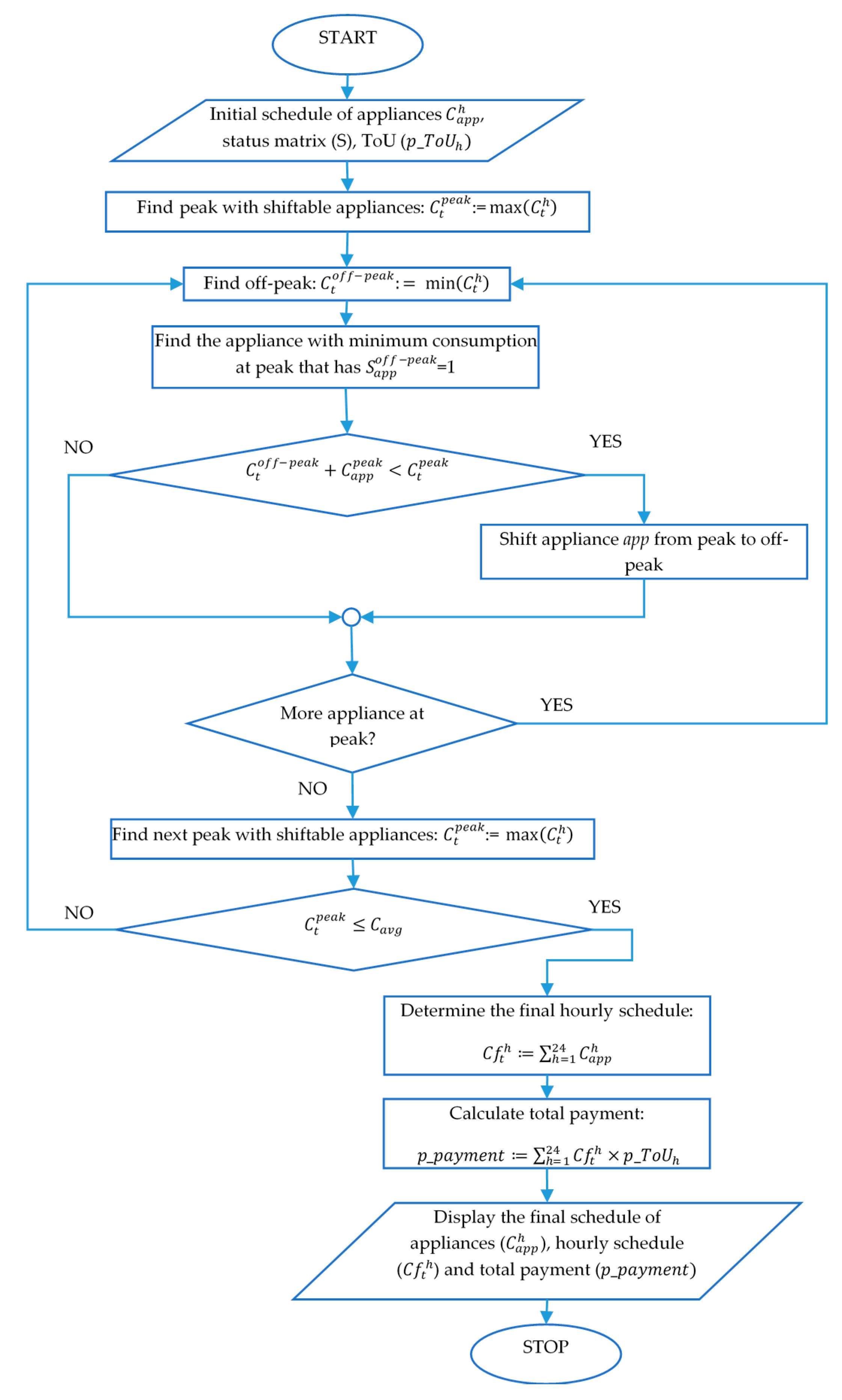
Shifting Algorithm 1 identifies peak and off-peak hours at each iteration. Then, the appliance with the smallest consumption (for the peak hour) is shifted from peak to off-peak hour by calling procedure SHIFT_APPLIANCE (app). This procedure is implemented in Oracle PLSQL based on Equations (2)–(7), depending on the type of shifted appliance (PIA or PNIA). The appliance will be shifted only if its status is on at off-peak hour indicated by the consumer in the status matrix S (). Otherwise, the next smallest programmable appliance is considered for shifting. Flowchart of the shifting Algorithm 1 is depicted in Figure 5.
We developed the algorithm as a stored procedure called LOAD_OPT_1 (p_C_type, p_Ci, p_S, p_ToU, p_Cf, p_payment), where p_C_type is the vector type of appliances, p_Ci is the matrix of initial consumption schedule, p_S represents status matrix of the programmable appliances and p_ToU is the ToU tariff hourly vector, p_Cf is the matrix of final consumption schedule (out parameter) and p_payment represents the total payment after shifting (out parameter).
| Algorithm 1 Gradual-shifting peak/off-peak algorithm |
| REPEAT REPEAT = UNTIL (=1) IF THEN CALL PROCEDURE SHIFT_APPLIANCE (app); ENDIF UNTIL |
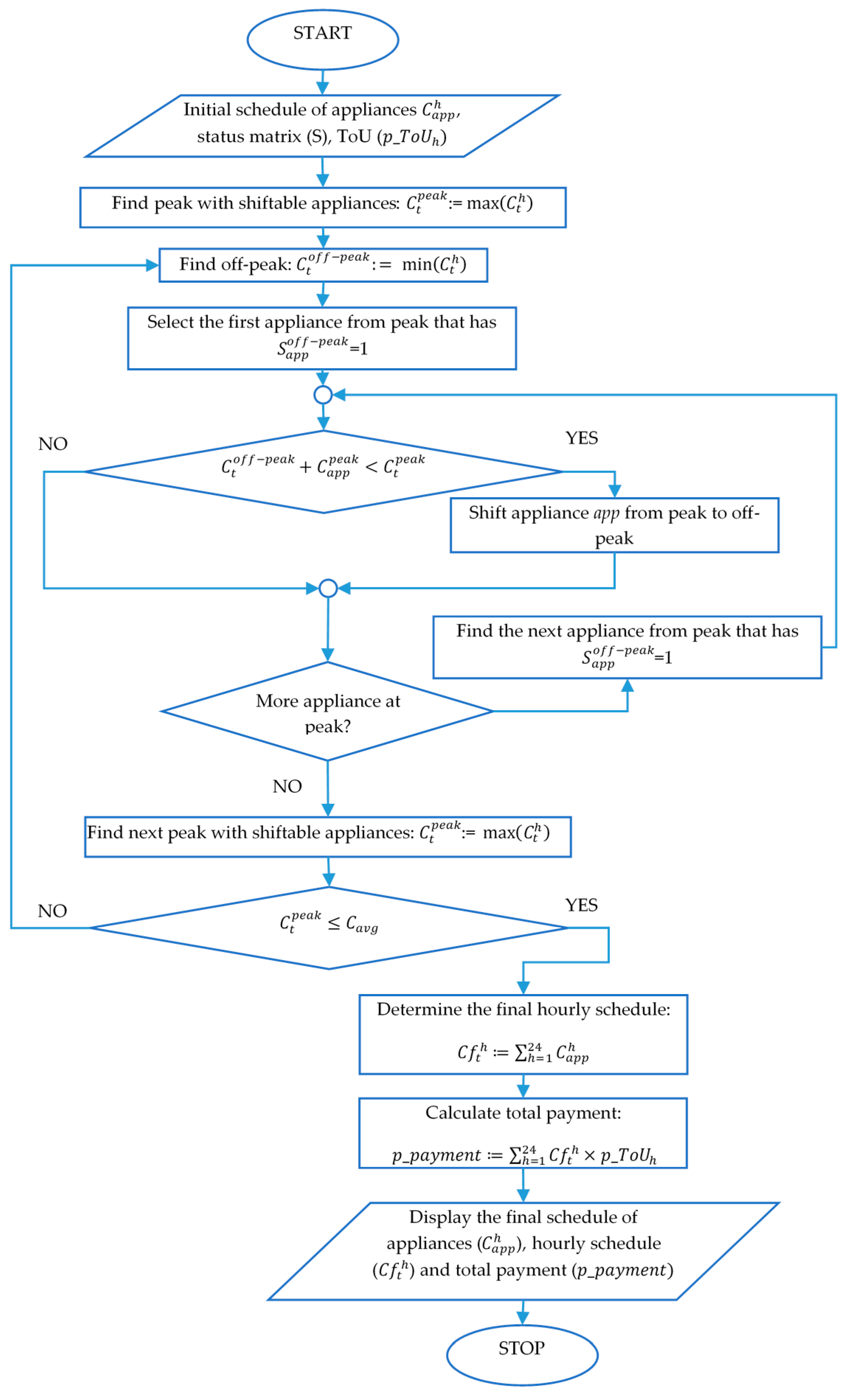
Shifting Algorithm 2 identifies consumption peak and shifts all programmable appliances to the consumption off-peak that is identified at each iteration. Flowchart of the shifting Algorithm 2 is depicted in Figure 6.
The algorithm is implemented in the procedure LOAD_OPT_2 (p_C_type, p_Ci, p_S, p_ToU, p_Cf, p_payment).
| Algorithm 2 Gradual-shifting off-peak algorithm |
| REPEAT WHILE appliance can be shifted from peak DO REPEAT = UNTIL (=1) IF THEN CALL PROCEDURE SHIFT_APPLIANCE (app); ENDIF ENDWHILE UNTIL |
Shifting Algorithm 3 identifies consumption peak and shifts all possible programmable appliances to the consumption off-peak. After shifting all programmable appliances, the consumption peak and off-peak hours are again identified and reiterate the process. Flowchart of the shifting Algorithm 3 is depicted in Figure 7.
We develop procedure LOAD_OPT_3 (p_C_type, p_Ci, p_S, p_Tou, p_Cf, p_payment) to implement the algorithm.
| Algorithm 3 Lump-shifting algorithm |
| REPEAT WHILE appliances can be shifted from peak TO off-peak DO IF =1 AND THEN CALL PROCEDURE SHIFT_APPLIANCE (app); ENDIF ENDWHILE UNTIL |
A comparative analysis of the results achieved by these three algorithms is performed in Section 5.
4.2. M2—Load Profiles Model. Self-Organizing Maps Algorithm for Load Profiles
The electricity consumption data hourly collected from 212 consumers’ apartments over one year is used to determine load profiles. Thus, we organize the input variables based on the type of consumption (heating, cooling, ventilation, indoor lighting etc.) and total consumption of each consumers. The variables are provided as vectors CL ∈ Rn, where n represents the number of inputs determined from consumption type and total consumption.
We develop a clustering algorithm based on self-organizing maps (SOM), an unsupervised learning that uses a neighborhood function for grouping inputs with similar behavior. This method builds groups/clusters based on distances between the neuron with the highest degree of similarity to the input vector and its neighbors. Self-organizing maps are matrix-based neural networks in which nodes are transformed accordingly to input vectors (classes). The algorithm performs in five steps, as follows:
Step 1: the network is initialized with random values for weight vectors of the nodes wi and an input vector CL(t) is chosen randomly from the training set;
Step 2: network parameters are configured:
- a neighborhood function Fcn (i, j, t) is chosen for determining the distances between neuron i and neuron j based on their similarities at each step t. It is recommended to establish a larger proximity (60–70%) for the first iterations that will be progressively reduced during learning;
- the learning rate is initialized. It represents a monotonically decreasing coefficient used for adjusting the distances between neurons;
- the network topology is chosen for setting up connections of the nodes;
- a number of maximum iterations (tmax) is provided for training.
Step 3: process each node in the map to find the similarity between the input vector and the weight vector of the map. The neighborhood function is applied and the neuron with the weight vector that is most similar to the input vector is chosen. This is called best matching unit (BMU).
Step 4: The weights of BMU and its neighbors are adjusted as follows:
Step 5: move to the next iteration t and repeat Step 3 until t = tmax or .
We implemented the SOM algorithm in Oracle PLSQL as a stored procedure called LOAD_PROF_SOM (tmax, nlayer, mlayer), where:
- tmax is the maximum number of iterations;
- nlayer and mlayer is the number of nodes representing dimension of the maps (nlayer × mlayer).
The procedure uses Euclidean distance for neighbourhood function Fcn (i, j, t).
4.3. M3—Consumption Forecast Model. ANN Algorithm for Consumption Forecast
Our proposed algorithm for consumption forecast is based on feedforward artificial neural networks (ANN) with backpropagation. The electricity consumption () can be determined by training the ANN on several instances of the input vector that consists of exogenous factors such as: temperature, wind speed, wind direction and humidity. Beside these factors, we may consider type of the day (working or week-end), hour and load profile of the consumer. These inputs are organized in the vector , , where m is the number of the input variables.
For the ANN architecture, we consider only one hidden layer H with p neurons and we use the activation function for the output layer as follows:
where:
- —bias of the hidden layer H;
- —represents the weight between the neuron j of hidden layer H and the output layer Y, ;
- —value of neuron j of the hidden layer H, determined as follows:
where:
- —activation function of the hidden layer;
- —bias of the input layer for each neuron of the hidden layer;
- —weight between each input neuron i and each neuron j of the hidden layer, and ;
For initializing the ANN parameters, we develop in Oracle PLSQL a stored procedure called INIT_ANN_LOAD (WX, BX, WH, bh, m, p), where WX and WH are arrays of weights, BX and bh represents biases, m is the number of inputs and p is the number of neurons of the hidden layer. The weights and biases are initialized with random values between 0 and 1.
In order to train the network, we standardize the input values with Min-Max method that scales the inputs to a fixed range of 0–1:
where:
- —minimum of all elements in the data set of each input ;
- —maximum of all elements in the data set of each input .
For standardization, we develop a procedure in Oracle PLSQL called MIN_MAX_ANN_LOAD().
The forecasting algorithm needs a proper training and validation steps and, in order to provide representative values for each step, we develop a procedure called SPLIT_ANN_LOAD (p_quota) that uses a hash function to randomly split the dataset in two parts, according to parameter p_quota.
During the training step, the weights and biases are progressively adjusted in order to fit the functions and . We consider the linear transfer approach for their implementation. The adjustments are made by minimizing the error function between the actual value of electricity consumption and the predicted value Y. The error function aggregates the errors for each pair of the training set :
The weights and biases are adjusted using a faster version of the gradient descend called Nesterov method. In this case the adjustments are made based on the gradients of the previous two iterations (t and t − 1):
where:
- —learning rate between 0 and 1;
- —direction of the gradient of at . is calculated for each weight and bias.
- —dynamic coefficient that starts with 1 and is iteratively updated based on calculated as:
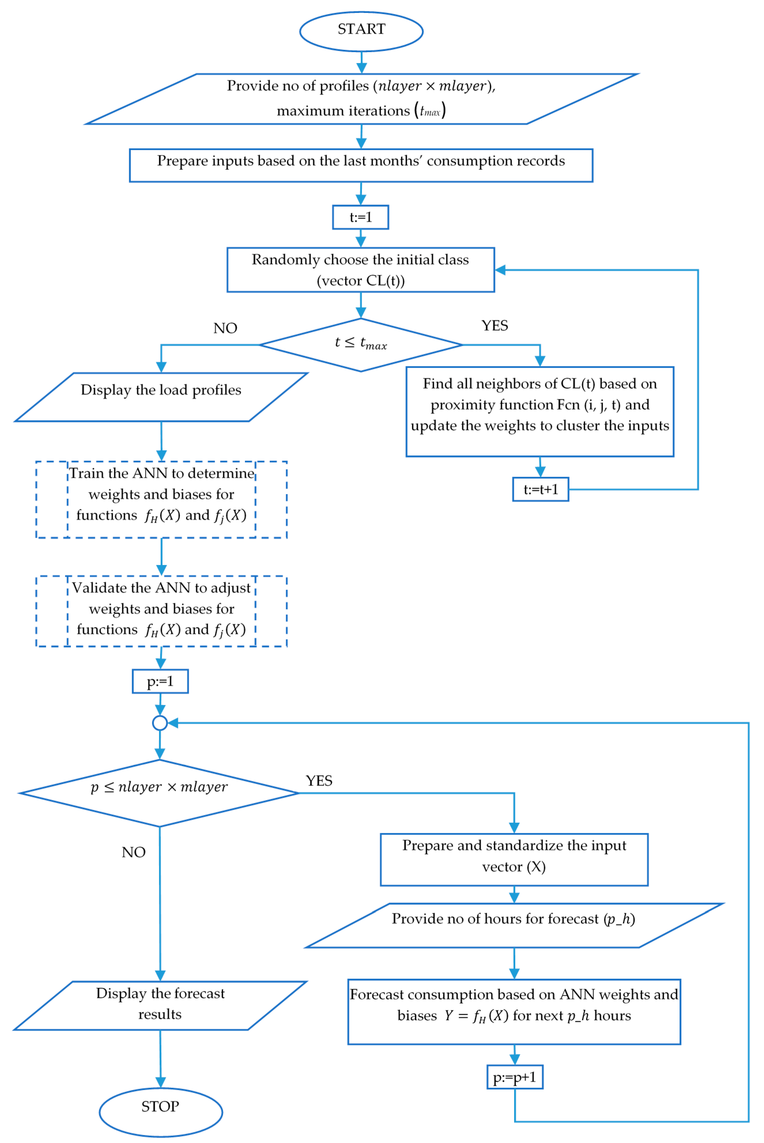
Since the forecasting algorithm is performed for each profile determined in model M2, flowchart of load profiles algorithm and consumption forecast algorithm is depicted in Figure 8. Training of the ANN is performed only once for a certain dataset, then once a month a validation process is performed to update the weights and biases based on the recent measurements. These steps are depicted in Figure 8 with dashed line.
For implementing the Nesterov method, we develop a stored procedure in Oracle PLSQL called TRAIN_ANN_LOAD (p_lr, max_epoch, eps) that initializes the learning rate with the value of p_lr. Parameter max_epoch limits the training of the ANN to a maximum number of iterations and eps provides the tolerated error.
The consumption forecast algorithm will provide the output for the next h hours based on the parameter of the procedure TEST_ANN_LOAD (p_h) developed for testing the algorithm.
5. Results
5.1. Testing the Optimization Algorithms
For optimizing the operation of the appliances, the consumer should provide only the day-ahead desirable schedule for all appliances (for simplicity, the individual consumption in Wh was divided by ten) based on their type as in Table 2 and the programmable appliances’ status matrix (S) or the possible operation time interval, where 1 is on and 0 is off as in Table 3. The consumption of all NPA is summed up since they cannot be involved in optimization process. Table 2 provide an example of a 24-h appliances’ schedule for four PIA and three PNIA
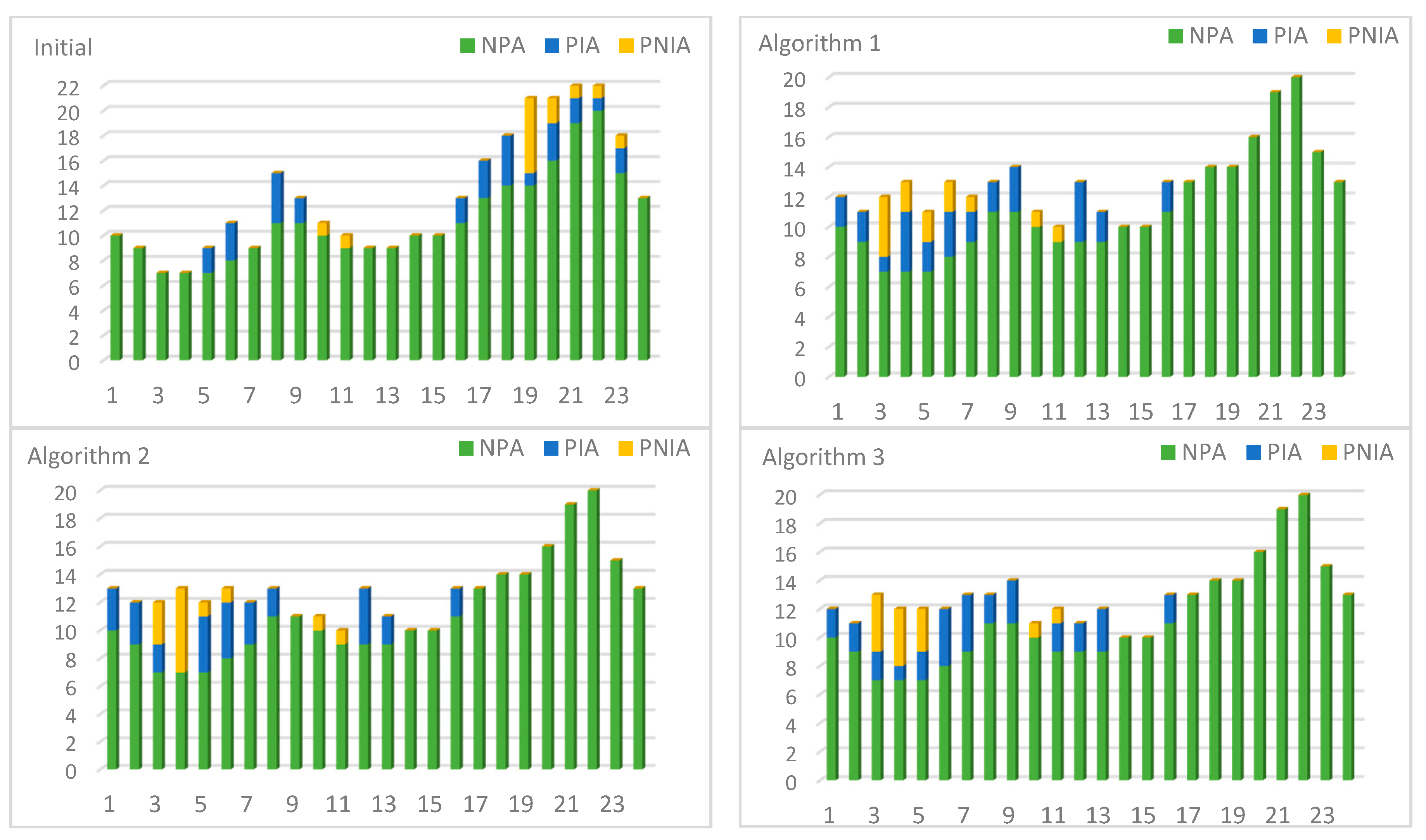
The proposed optimization algorithms identically shifts the programmable appliances from peak to off-peak hours, according to Figure 9, the differences appear at the off-peak hours. However, after optimization, the hourly consumption peak reduction is between 9.1% (at hour 22) and 33% (at hour 19).
The Algorithms 1 and 3 are similar, while the Algorithm 2 better deals with flattening the consumption especially at the off-peak hours.
From Figure 10 it can be noticed that PIA and PNIA appliances that operate at peak are shifted to off-peak hours according to the proposed algorithms.
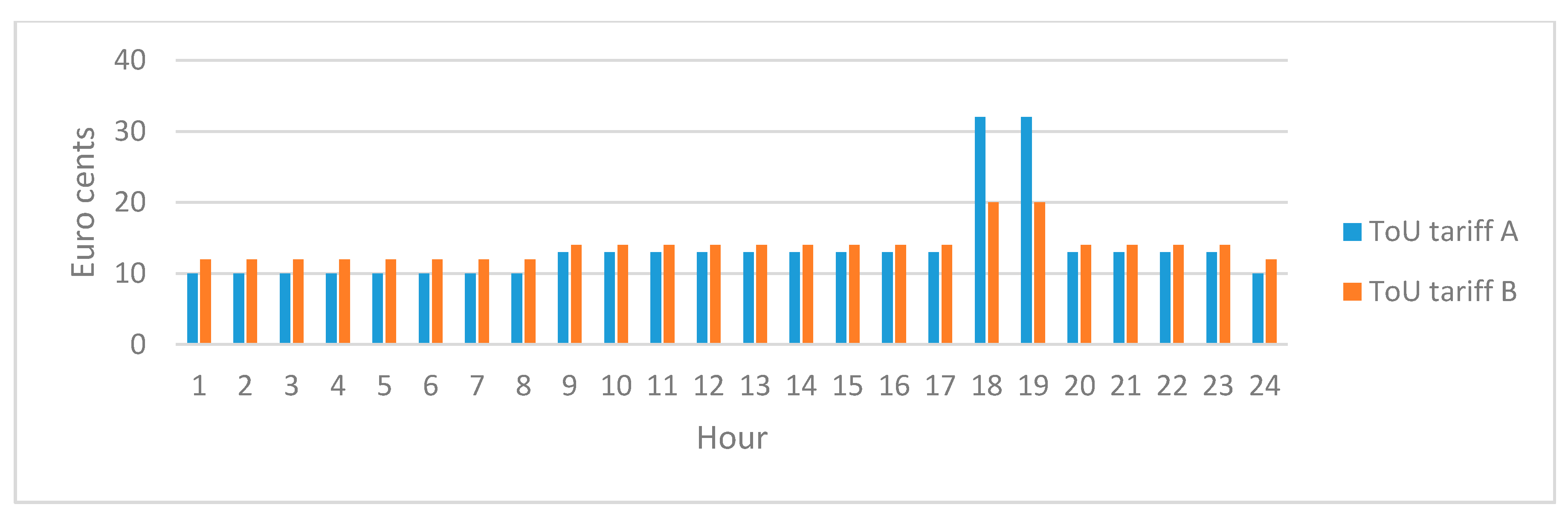
For payment evaluation, we consider two ToU tariffs as in Figure 11 that are applied to the optimized hourly consumption. ToU tariff A discourages the consumption at peak hours (18, 19) being significantly higher than ToU tariff B, but for the rest of the day, it is slightly smaller than ToU tariff B. Both tariffs encourage the night electricity consumption when the tariff is lower. Based on the simulation results, the supplier may transparently choose to implement a specific tariff that is the most convenient for the electricity consumer.
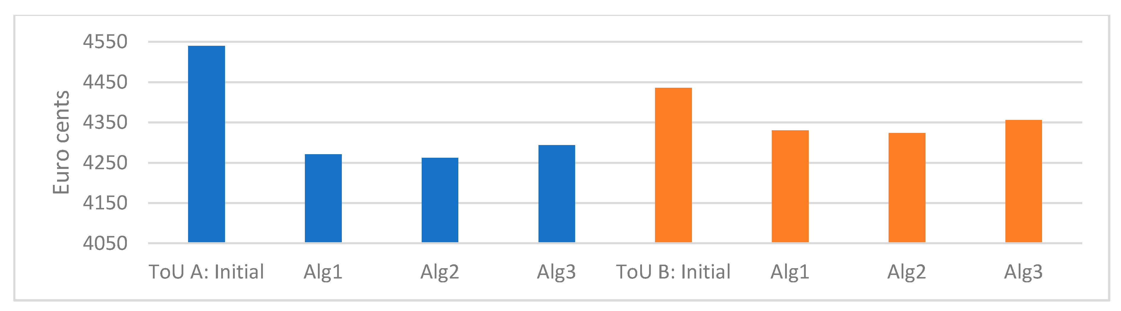
Then, in Figure 12 we show the payment for electricity consumption considering the results of the optimization algorithms and the above ToU tariffs. It results that regardless the ToU tariff, the least expensive case is given when Algorithm 2 is applied.
Although, the three algorithms ensure a consumption peak reduction between 9.1% and 33%, considering the two ToU tariffs, they generate different electricity payments. Further adjustable operation of appliances such as air-conditioning, lighting and heating could be considered to increase the flatness of the load curve. Therefore, for these scenarios, the most expensive algorithm is the third one, while the most rapid algorithm for electricity consumers is the second one; it also provides more savings. Through the web-service interface, the consumers run in parallel all three algorithms, analyze the results and choose the most convenient option in terms of payment.
According to Table 4, the second algorithm with ToU A tariff provides the biggest savings (6.12%). Also the implementation of these algorithms is done with different number of iterations as in Table 4.
From Table 4, we can conclude that ToU A is the most convenient tariff for householder that can be stimulated to shift the operation of the programmable appliances for financial incentives.
5.2. Testing the Load Profile Algorithm
For simulations on the set of 212 consumers’ data, we set the maximum number of iterations tmax = 1000; as for the number of neurons, we test three scenarios: (i) 3 × 3; (ii) 2 × 3 and (iii) 2 × 2. For each option, we run the algorithm and analyse the results.
- (i)
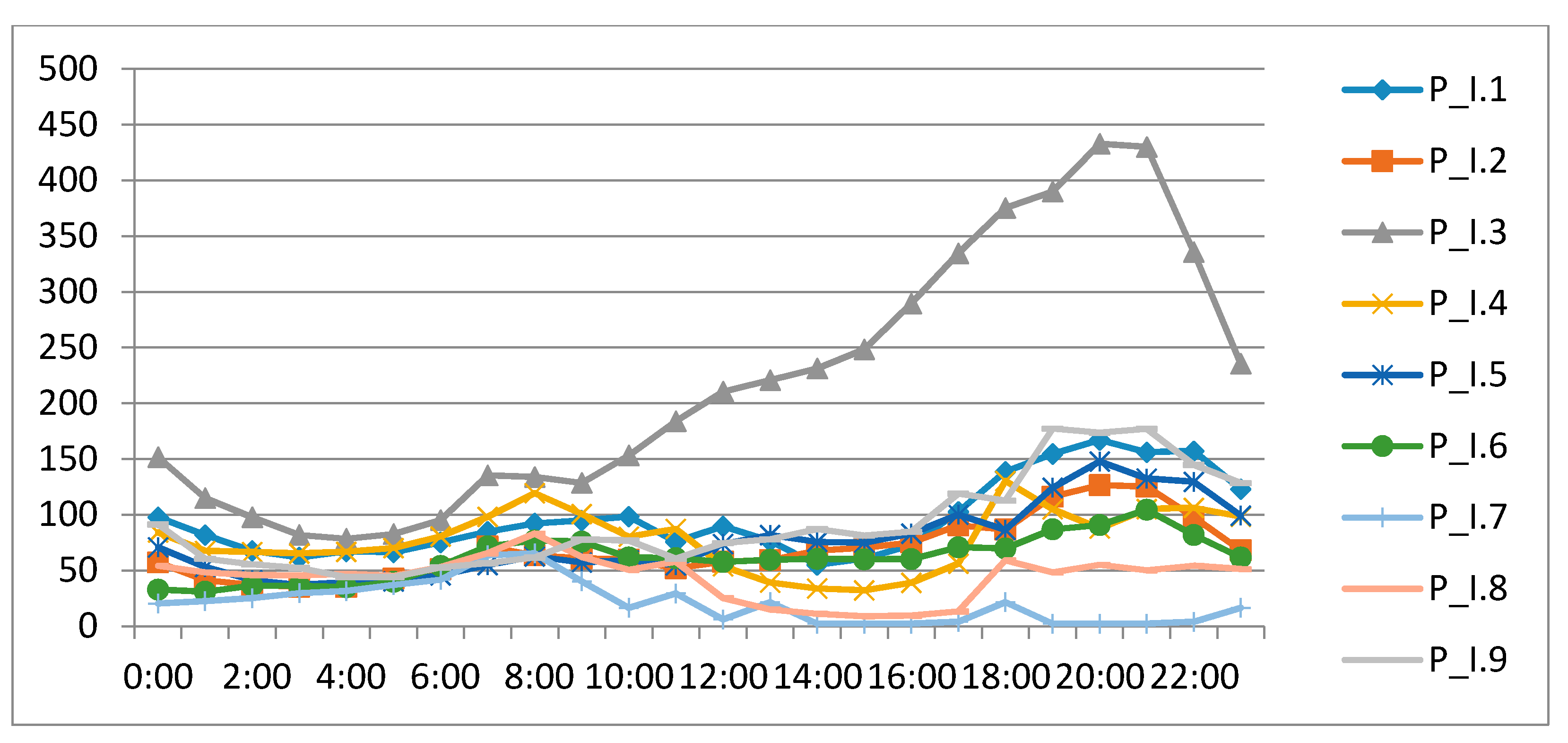
- In the first scenario, the algorithm determined nine load profiles (P_I.1, …, P_I.9) as in Figure 13, where we can observe that there are similarities between several profiles (P_I.1, P_I.2, P_I.4, P_I.5, P_I.6, P_I.9) and only P_I.3, P_I.7 and P_I.8 are well-delimited from other profiles. Also, the most profiles differ only in the amplitude (peak or off-peak consumption level), except P_I.3, P_I.7 and P_I.8 which have a different consumption pattern.
- (ii)
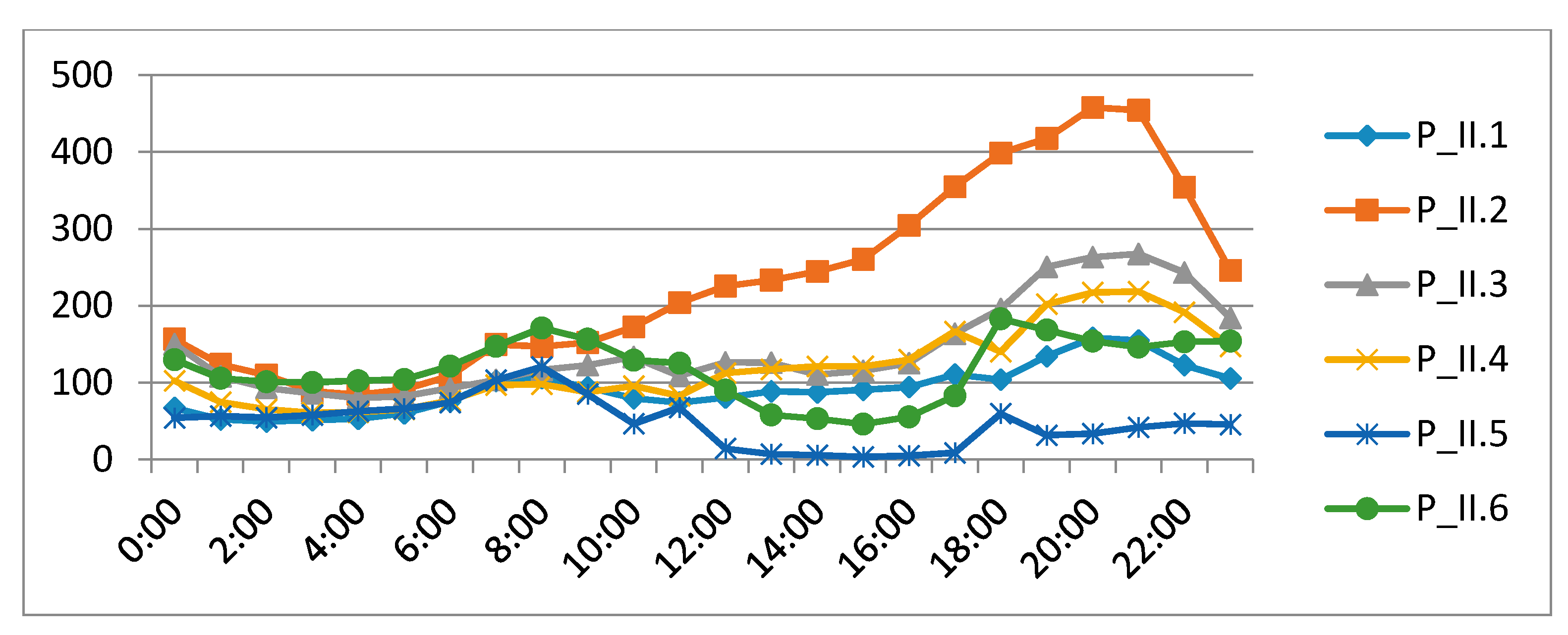
- In the second scenario, we determine six load profiles on a 2 × 3 layers architecture that are shown in Figure 14. Profiles P_I.1, P_I.2, P_I.4, P_I.5, P_I.6, P_I.9 from the first scenario with similar consumption patterns are clustered in 4 profiles better delimited. Also, P_I.3 from the first scenario maintains its cluster, now P_II.2. P_I.7 and P_I.8 from the first scenario are now grouped in one profile, P_II.5. Therefore, this scenario offers better delimitation of the load profiles and provides a more accurate overview over groups of consumers.
- (iii)
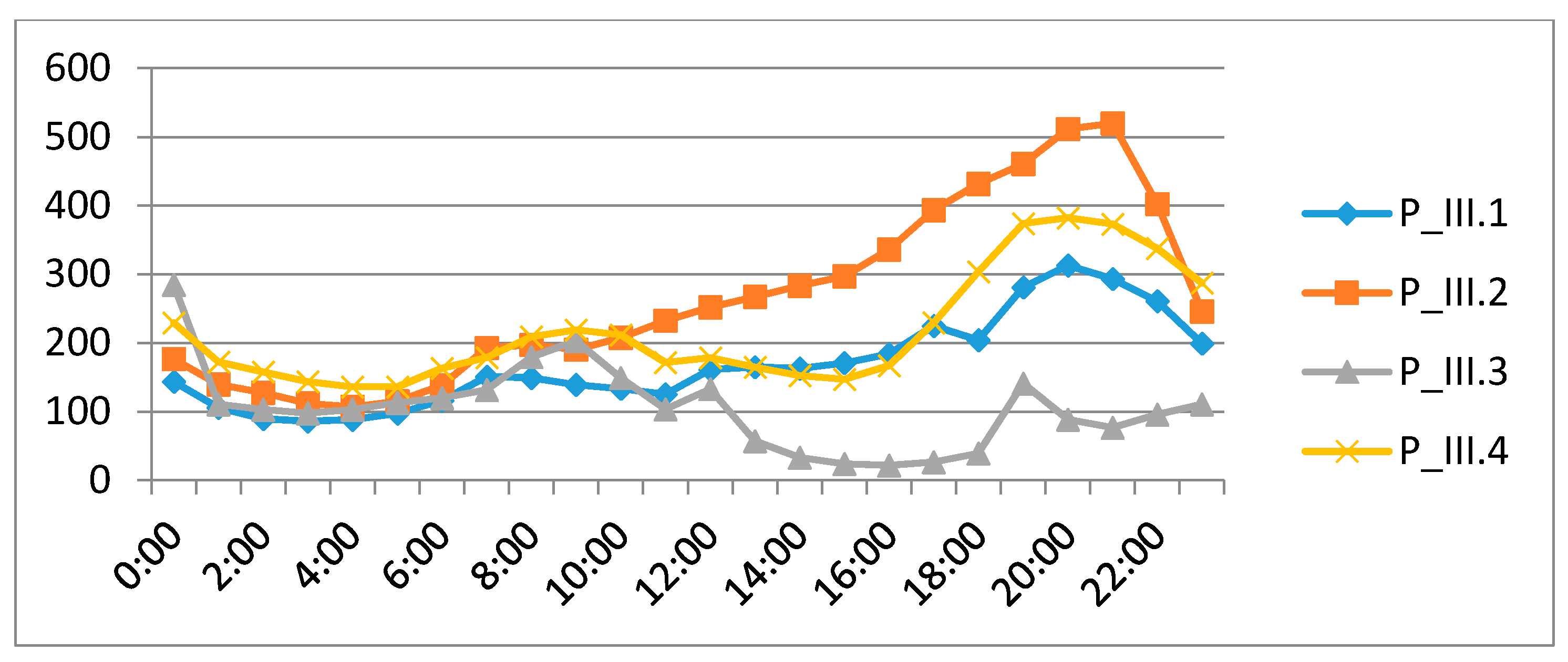
- The third scenario determines four load profiles as depicted in Figure 15. As it can be observed, P_II.2 maintains its place and also P_II.5 from the second scenario. P_III.3 increases its members by adding some members from P_II.6 and P_II.1 from the second scenario. P_III.1 and P_III.4 include members from previous P_II.1 and P_II.6, respectively P_II.3 and P_II.4.
This scenario offers a better delimitation than the second scenario, but in case the electricity supplier needs a more detailed perspective over consumers’ segmentation, the second scenario can be applied. As a consequence, we decided to develop a comparative analysis section in the web-service interface to allow the electricity supplier to visualize, compare and decide over the number of load profiles that can be achieved.
5.3. Testing the Consumption Forecast Algorithm
Simulations are performed on the 212-consumer dataset and, in addition to consumption measurements, we add hourly recorded weather data for temperature, humidity, wind speed and wind direction. Also, we add as inputs three more variables: type of day (working or weekend), hour and cluster (load profile) determined with LOAD_PROF_SOM procedure. The input vector X has the following structure:
where:
- —temperature;
- —humidity;
- —wind speed;
- —wind direction;
- —type of day, ;
- —hour, ;
- —profile, or depending on the electricity supplier’s option.
The output Y is the total electricity consumption of each cluster. For estimating the accuracy, we use root-mean-square error (RMSE) and correlation coefficient (R), the results being centralized in Table 5 for each cluster, testing for the 4 profiles scenario.
In Figure 16, the consumption forecast for profile P_III.1 is compared with the actual consumption. The error is also depicted.
Consumption forecast algorithm is re-validated at every 30 days in order to update its weights and biases with the newest inputs for weather conditions and consumers’ profiles. Thus, any potential change in the consumer behavior is reflected in the load profiles and then in the forecasting algorithm.
6. Interfaces of the Prototype
In order to implement the informatics prototype that is mainly designed to serve the requirements of consumers and electricity suppliers/grid operators, we used the following technologies: Oracle Database 12c for data management, including development of stored procedures described in Section 4, and Oracle JDeveloper 12c with Application Development Framework (ADF) for developing the web-services interfaces. Users access the web-services through online interfaces integrated in a web portal. Each type of user (electricity consumer, supplier or grid operator) may access the portal and interact with customized interfaces.
The electricity consumers access their individual ECMI available in the portal to manage consumption places and visualize the allocated electricity tariffs. Also, they can configure appliances by setting the type of each appliance and hourly consumption (page Scheduler of the portal). In addition, the status matrix of the programmable appliances is also required by the shifting algorithms. After configuration of appliances, consumers access the optimization model M1 (Consumption optimization page). The shifting algorithms are run in parallel, the final schedule and total payment are generated for each algorithm. Consumers choose the best option that minimize the consumption payment. However, the results in terms of savings and peak reduction depend on the flexibility of each consumer and share of programmable appliances.
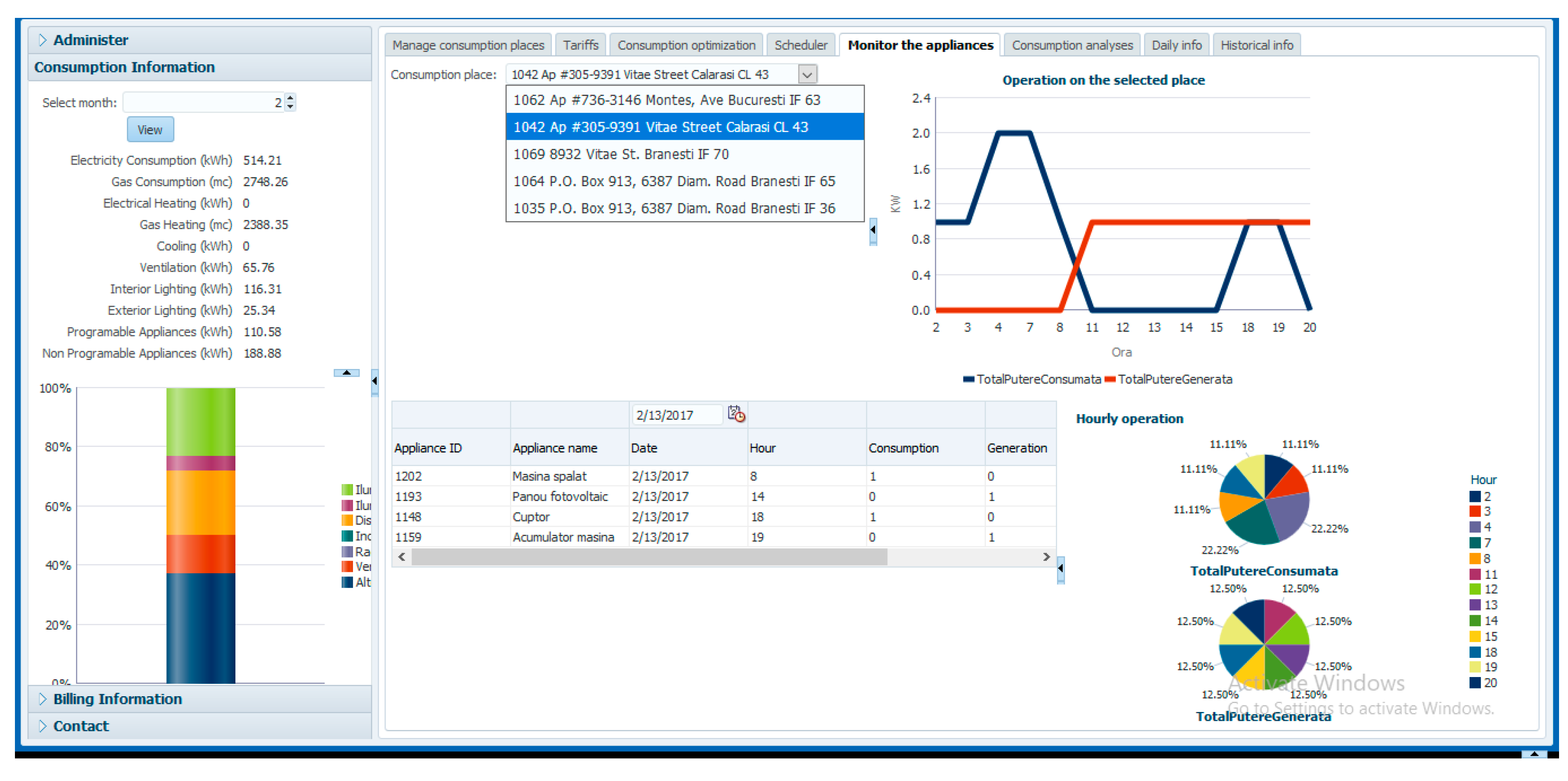
In Figure 17 (page Monitor the appliances), the consumers monitor the electricity consumption by category of consumption (left section of the page) during a selected period and visualize hourly operation of appliances for a given consumption place that can be also selected from a list (top-right section of the page). Also, the hourly consumption data for each appliance is depicted (bottom section of the page). Since the operation of each appliance is displayed, its share can be analyzed and the consumer may identify the energy intensive appliances and choose to replace them and therefore decrease the electricity consumption.
Other pages of the ECMI portal provide access to tariffs, consumption analyses over types of appliances, daily and historical analyses of consumption with charts, tables, selectors and gauges.
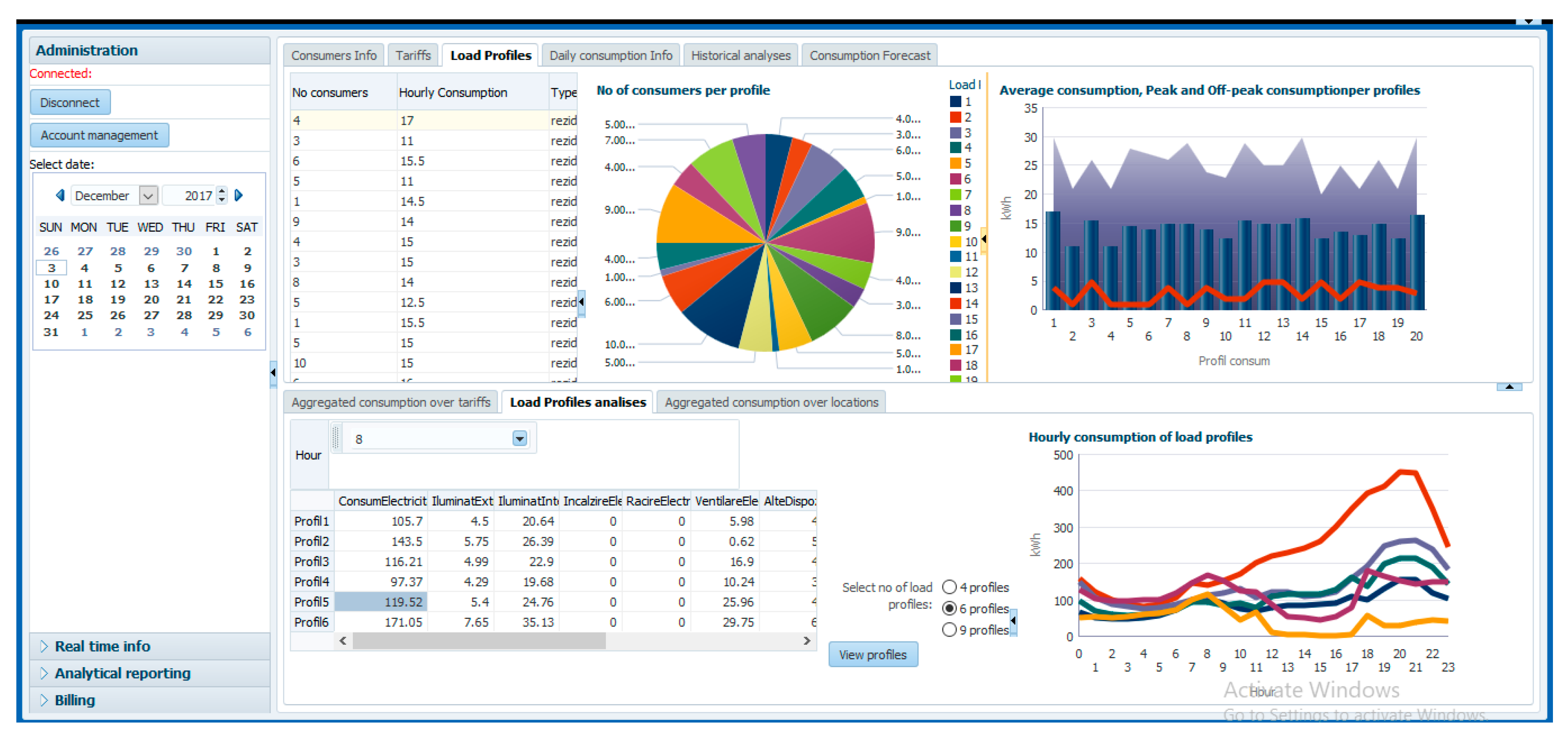
The electricity supplier accesses the CC through the portal interfaces (Figure 18) to manage consumers data (page Consumers Info) and set up tariffs for consumers (page Tariffs). Also, the supplier accesses model M2 (page Load Profiles) to select the number of profiles and run the load profile algorithm (bottom section of the page), visualizing the number of consumers that belong to each profile and their average, peak and off-peak consumption (top section of the page).
Moreover, the supplier analyses the distribution of the average, peak and off-peak consumption for a selected date and hour by customizing the pivot table from the bottom of the page.
The electricity supplier can also analyse consumption for each place or over aggregated locations (in page Daily consumption info) and can perform historical analyses (page Historical analyses) by comparing the actual consumption with records of the previous days. The hourly electricity consumption can be analysed based on types of appliances.
In Consumption Forecast page, the electricity supplier accesses model M3 to run the consumption forecast algorithm selecting the corresponding number of hours to forecast. Then, the accuracy of the model can be calculated for previous forecasts.
Other portal sections provide access to billing system, real-time distribution of the consumption over types of appliances and analytical reports for advanced analyses over locations, type of consumers and profiles.
The portal is currently under development and partially tested by an electricity supplier with 5% market share in Romania. The development involves prosumers, extending the type of appliances, other utilities integration, electric vehicles and improving the optimization algorithms by considering not only shifting, but also adjusting of some appliances. In order to facilitate the use of portal, we also consider to introduce algorithms that can provide suggestion for day-ahead schedule based on consumption patterns.
7. Discussion
Consumption optimization brings significant benefits to consumers, suppliers and grid operators since it reduces the investment requirements related to onerous grid infrastructure. Based on advanced tariffs and other DSM measures, the consumers become more and more active and are motivated to schedule their appliances. For consumption optimization, we propose three algorithms that shift the programmable appliances to flatten the peak, since by this objective, multiple benefits can be achieved by the electricity consumers, suppliers and grid operators. It will also lead to the reduction of electricity consumption payment due to the fact that at off-peak hours the tariff is lower; some investment in grid facilities can be avoided or postponed; the suppliers’ acquisition market strategies will be improved; losses will be reduced; and generators are less stressed. The mere objective of diminishing the electricity payment by shifting the appliances from high rate to low rate tariff intervals is only a temporary solution since new peaks may emerge and thus always new design of ToU tariff is required. Usually, the reduction of electricity payment does not lead to the reduction of peak consumption; on the contrary the peak can be higher than without optimization.
Electricity suppliers combine the optimal schedule with advanced tariffs such as ToU, critical pricing or real-time tariffs that encourage the consumption at off-peak hours. Based on the design of advanced tariffs, the consumers will change their behavior and shift the operation of the appliances accordingly. Therefore, we compare the results of the three algorithms combined with two ToU tariffs. The proposed algorithms shift the programmable appliances from peak to off-peak hours, with significant changes at the off-peak hours. The hourly consumption in the evening when peak occurs decreases between 9.1% (at hour 22) and 33% (at hour 19). For payment evaluation, it results that, the least expensive case is given when Algorithm 2 is applied (6.12% savings with ToU A tariff). Also, Algorithm 2 is the most rapid (lowest number of iterations). Shifting Algorithm 2 identifies consumption peak and shifts all programmable appliances to off-peak hour that is identified at each iteration, while ToU tariff A discourages the consumption at peak hours, but for the rest of the day, it is slightly smaller than ToU tariff B. Regardless the shifting algorithm, the biggest savings are recorded by implementing the ToU tariff A, therefore the consumers are rewarded when they shift the appliances from peak to off-peak hours. We may conclude that Algorithm 2 in combination with ToU A tariff are the most convenient for householder that can be stimulated to shift the operation of the programmable appliances for financial incentives.
For obtaining consumption profiles, we develop a clustering algorithm based on self-organizing maps. By running the algorithm for three scenarios, different well-delimited profiles are performed. Thus, through the prototype’s interface, the supplier can choose to visualize a different number of profiles that are input data in consumption forecast. As for the consumption forecast, feedforward artificial neural networks algorithm with backpropagation is implemented. High accuracy of the results helps supplier to improve market strategy. It also helps grid operators to better plan grid capacity and other resources. Finally, we test algorithms showing their performance and integrate them into an informatics solution as a prototype. This solution can be replicated on other database platforms, even on open source platforms, by implementing the algorithms in other programming languages. To support the replication, we provide detailed flowcharts for the proposed algorithms, refine the main flowchart of the methodology and describe the interaction among the components and architecture of the prototype.
As a further development of our prototype, we consider to include prosumers’ activities and also the effect of electrical vehicles and storage systems will be analyzed. Moreover, we will consider the heat pumps, with additional datasets provided by sensors for measuring the interior temperature and humidity.
However, regardless the incentives provided by supplier, some consumers will not change their behavior. By offering an easy to use mobile or web-serviced applications that are less time-consuming and user-friendly, the share of reluctant consumers may decrease. Based on data mining algorithms, the application can suggest possible day-ahead schedule of appliances and the tasks of consumers will be diminished; they only have to confirm or make minor modifications. Therefore, we will consider data mining algorithms for suggestions of scheduling to improve our prototype.
8. Conclusions
In this paper, we present an informatics solution for consumption management that assists consumers, suppliers and grid operators in finding the best decisions regarding consumption optimization and forecast, identification of intensive appliances and profiles. Also, the solution leads to both peak consumption and payment minimization, improves the consumption forecast accuracy and increases the awareness regarding the consumption management. The solution is developed based on web-services that offer friendly interfaces, both consumers and suppliers/grid operators being able to visualize data through interactive controls such as reports, pivot tables, charts, maps, scenarios and various gauges. It comprises three models for consumption optimization, profiles clustering and forecasts that mainly use input consumption data from smart meters and sensors.
As a novelty, the input data is transformed and loaded into a relational cloud database and also the proposed algorithms are implemented as stored procedures in the same database, increasing the performance of the processing algorithms, avoiding additional software tools for implementation.
For energy efficiency improvement, we propose to shift appliances to reduce the peak consumption and increase savings by avoiding onerous cost related to additional grid infrastructure. Moreover, by this solution, the consumers are able to monitor electricity consumption at the appliance level and identify the energy intensive appliances that can be replaced to reduce the electricity consumption and further increase the savings. Also, by our approach, the consumption profiles and forecast aim to increase the predictability of the consumption, improve the market strategies of suppliers that lead to electricity tariff reduction and enable sustainable development of power systems.
Acknowledgments
This work is supported by a grant of the Romanian National Authority for Scientific Research and Innovation, CNCS/CCCDI—UEFISCDI, project number PN-III-P2-2.1-BG-2016-0286 “Informatics solutions for electricity consumption analysis and optimization in smart grids” and contract No. 77BG/2016, within PNCDI III.
Author Contributions
S.-V.O. designed the shifting algorithms, implemented algorithms in the prototype and wrote the paper. A.B. designed the forecast and profiles clustering algorithms, contributed to implementation of the algorithms in the prototype and wrote the paper. A.R. contributed to the literature review and aspects related to interfaces of the prototype.
Conflicts of Interest
The authors declare no conflict of interest.
References
- European Commission, Climate Action, 2020 Climate & Energy Package. Available online: https://ec.europa.eu/clima/policies/strategies/2020_en (accessed on 8 September 2017).
- Eurostat, Electricity Production, Consumption and Market Overview. Available online: http://ec.europa.eu/eurostat/statistics-explained/index.php/electricity_production,_consumption_and_market_overview (accessed on 10 September 2017).
- EUREL Convention of National Associations of Electrical Engineers of Europe, Electrical Power Vision 2040 for Europe. Available online: http://www.eurel.org/home/TaskForces/Documents/EUREL-PV2040-Short_Version_Web.pdf (accessed on 15 September 2017).
- Entso-E Scenario Outlook & Adequacy Forecast 2015. Available online: https://www.entsoe.eu/Documents/SDC%20documents/SOAF/150630_SOAF_2015_publication_wcover.pdf (accessed on 20 September 2017).
- Electric Power Research institute (EPRI), Assessment of Achievable Potential from Energy Efficiency and Demand Response Programs in the U.S. (2010–2030). Available online: http://www.edisonfoundation.net/IEE/Documents/EPRI_AssessmentAchievableEEPotential0109.pdf (accessed on 17 September 2017).
- Oprea, S.V.; Bâra, A.; Cebeci, E.M.; Tor, O.B. Promoting peak shaving while minimizing electricity consumption payment for residential consumers by using storage devices. Turk. J. Electr. Eng. Comput. Sci. 2017, 25. [Google Scholar] [CrossRef]
- Oprea, S.V. Informatics solutions for electricity consumption optimization. In Proceedings of the 16th IEEE International Symposium on Computational Intelligence and Informatics—CINTI 2015, Budapest, Hungary, 19–21 November 2015. [Google Scholar]
- Oprea, S.V.; Bâra, A. Electricity load profile calculation using self-organizing maps. In Proceedings of the 20th International Conference on System Theory, Control and Computing (ICSTCC), Sinaia, Romania, 13–15 October 2016; pp. 860–865. [Google Scholar]
- Oprea, S.V.; Bâra, A.; Lungu, I. Methods for electricity load profile calculation within deregulated markets. In Proceedings of the 19th International Conference on System Theory, Control and Computing Joint Conference SINTES 19, Comuna Fundata, Romania, 14–16 October 2015; pp. 848–853. [Google Scholar]
- Optimus Decision Support System. Available online: http://www.optimus-smartcity.eu/ (accessed on 17 September 2017).
- Optimising Energy Use in Cities through Smart Decision Support Systems. Available online: http://www.50001seaps.eu/fileadmin/user_upload/Open_Training_Session_EUSEW_2015/5_OPTIMUS_Z%C3%B6llner.pdf (accessed on 30 August 2017).
- Kewo, A.; Munir, R.; Lapu, A.K. IntelligEnSia based Electricity Consumption Prediction Analytics using Regression Method. In Proceedings of the 2015 International Conference on Electrical Engineering and Informatics (ICEEI), Bali, Indonesia, 10–11 August 2015. [Google Scholar]
- Hylton, O.; Tennant, V.; Golding, P. The Impact of a ZigBee Enabled Energy Management System on Electricity Consumption, Energy Management System using ZigBee. In Proceedings of the 19th Americas Conference on Information Systems (AMCIS), Chicago, IL, USA, 15–17 August 2013. [Google Scholar]
- Khodaei, A.; Shahidehpour, M.; Choi, J. Optimal Hourly Scheduling of Community-Aggregated Electricity Consumption. J. Electr. Eng. Technol. 2013, 8, 1251–1260. [Google Scholar] [CrossRef]
- Logenthiran, T.; Srinivasan, D.; Shun, Z. Demand Side Management in Smart Grid Using Heuristic Optimization. IEEE Trans. Smart Grid 2012, 3, 1244–1252. [Google Scholar] [CrossRef]
- Bonfiglio, A.; Delfino, F.; Invernizzi, M.; Procopio, R. A Methodological Approach to Assess the Impact of Smarting Action on Electricity Transmission and Distribution Networks Related to Europe 2020 Targets. Energies 2017, 10, 155. [Google Scholar] [CrossRef]
- López-González, L.M.; López-Ochoa, L.M.; Las-Heras-Casas, J.; García-Lozano, C. Final and primary energy consumption of the residential sector in Spain and La Rioja (1991–2013), verifying the degree of compliance with the European 2020 goals by means of energy indicators. Renew. Sustain. Energy Rev. 2017, 81, 2358–2370. [Google Scholar] [CrossRef]
- Bel, G.; Joseph, S. Climate change mitigation and the role of technological change: Impact on selected headline targets of Europe’s 2020 climate and energy package. Renew. Sustain. Energy Rev. 2018, 82, 3798–3807. [Google Scholar] [CrossRef]
- Fura, B.; Wojnar, J.; Kasprzyk, B. Ranking and classification of EU countries regarding their levels of implementation of the Europe 2020 strategy. J. Clean. Prod. 2017, 165, 968–979. [Google Scholar] [CrossRef]
- Liobikienėa, G.; Butkusb, M. The European Union possibilities to achieve targets of Europe 2020 and Paris agreement climate policy. Renew. Energy 2017, 106, 298–309. [Google Scholar] [CrossRef]
- Warren, P. The Potential of Smart Technologies and Micro-Generation in UK SMEs. Energies 2017, 10, 1050. [Google Scholar] [CrossRef]
- Godina, R.; Rodrigues, E.M.G.; Pouresmaeil, E.; Catalão, J.P.S. Optimal residential model predictive control energy management performance with PV microgeneration. Comput. Oper. Res. 2017. [Google Scholar] [CrossRef]
- Jiang, B.; Fei, Y. Smart home in smart microgrid: A cost-effective energy ecosystem with intelligent hierarchical agents. IEEE Trans. Smart Grid 2015, 6, 3–13. [Google Scholar] [CrossRef]
- Pîrjan, A.; Oprea, S.V.; Cărutăsu, G.; Petrosanu, D.M.; Bâra, A.; Coculescu, C. Devising Hourly Forecasting Solutions Regarding Electricity Consumption in the Case of Commercial Center Type Consumers. Energies 2017, 10, 1727. [Google Scholar] [CrossRef]
- Mogles, N.; Walker, I.; Ramallo-González, A.P.; Lee, J.H.; Nataraj, S.; Padget, J.; Gabe-Thomas, E.; Lovett, T.; Rena, G.; Hyniewska, S.; et al. How smart do smart meters need to be? Build. Environ. 2017, 125, 439–450. [Google Scholar] [CrossRef]
- Javaid, N.; Hussain, S.M.; Ullah, I.; Noor, M.A.; Abdul, W.; Almogren, A.; Alamri, A. Demand Side Management in Nearly Zero Energy Buildings Using Heuristic Optimizations. Energies 2017, 10, 1131. [Google Scholar] [CrossRef]
- Palensky, P.; Dietrich, D. Demand Side Management: Demand Response, Intelligent Energy Systems, and Smart Loads. IEEE Trans. Ind. Inform. 2011, 7, 381–388. [Google Scholar] [CrossRef]
- Apajalahti, E.L.; Lovio, R.; Heiskanen, E. From demand side management (DSM) to energy efficiency services: A Finnish case study. Energy Policy 2015, 81, 76–85. [Google Scholar] [CrossRef]
- Barbato, A.; Capone, A. Optimization models and methods for demand-side management of residential users: A survey. Energies 2014, 7, 5787–5824. [Google Scholar] [CrossRef]
- Tan, X.; Shan, B.; Hu, Z.; Wu, S. Study on demand side management decision supporting system. In Proceedings of the 2012 IEEE 3rd International Conference on Software Engineering and Service Science (ICSESS), Beijing, China, 22–24 June 2012. [Google Scholar]
- Duah, D.; Syal, M. Intelligent decision support system for home energy retrofit adoption. Int. J. Sustain. Built Environ. 2016, 5, 620–634. [Google Scholar] [CrossRef]
- Smart Metering in Romania. Available online: http://www.anre.ro/download.php?f=gKp%2BhA%3D%3D&t=vdeyut7dlcecrLbbvbY%3D (accessed on 15 December 2017).
- Berges, M.; Rowe, A. Appliance classification and energy management using multi-modal sensing. In Proceedings of the Third ACM Workshop on Embedded Sensing Systems for Energy-Efficiency in Buildings, Seattle, WA, USA, 1–4 November 2011. [Google Scholar]
Figure 1.
Electricity consumption management components.

Figure 2.
Architecture of the prototype.

Figure 3.
Flowchart of the models and algorithms.

Figure 4.
Types of programmable appliances.

Figure 5.
Flowchart of the shifting Algorithm 1.

Figure 6.
Flowchart of the shifting Algorithm 2.

Figure 7.
Flowchart of the shifting Algorithm 3.

Figure 8.
Flowchart of load profiles algorithm and consumption forecast algorithm.

Figure 9.
Initial and optimized daily consumption considering the three algorithms.

Figure 10.
Consumption of different type of appliances for initial schedule and shifting algorithms.
Figure 10.
Consumption of different type of appliances for initial schedule and shifting algorithms.

Figure 11.
Time-of-use tariffs.

Figure 12.
Daily electricity payment.

Figure 13.
Load profiles obtained with 3 × 3 architecture.

Figure 14.
Load profiles obtained with 2 × 3 architecture.

Figure 15.
Load profiles obtained with 2 × 2 architecture.

Figure 16.
Load forecasted values versus actual consumption for profile P_III.1.

Figure 17.
Appliances operation programming.

Figure 18.
Consumption profiles management.


Table 1.
Interaction between users and models.
| Users | Electricity Supplier | Electricity Consumers | |
|---|---|---|---|
| Model Execution | |||
| M1—Consumption optimization | 1. Provides ToU tariffs; 7. Visualises the load schedule for individual/aggregated consumers based on optimization model. | 2. Set appliances type; 3. Provide initial schedule of appliances and status options of programmable appliances for the next day; 4. Optimize consumption for next day by running in parallel three shifting algorithms; 5. Analyse the optimized schedule of appliances and total payment for the next day; 6. Select the best schedule that minimizes the payment and save it to ECMI and central database; | |
| M2—Load profiles | 1. Selects the number of load profiles; 2. Executes the clustering algorithm at least once a month with data collected from previous 3 months; 3. Stores the results in the Control Centre (central database); 4. Analyses the profiles and distribution of total consumption for each profile; | 5. Access the ECMI and visualise own profile information and compare consumption with similar profile. | |
| M3—Consumption forecast | 1. Trains the ANN network with historical data (this step is performed only once); 2. Validates ANN with previous 30 days records (this step is performed periodically, every month); 3. Provides the forecast period (number of hours); 4. Executes the consumption forecast algorithm for each load profile; 5. Analyses the output and compare actual values with forecasts for each profile and for aggregated consumption; | 6. Visualize estimated consumption for own profile. | |
Table 2.
Initial consumption schedule.
| App | 1 | 2 | 3 | 4 | 5 | 6 | 7 | 8 | 9 | 10 | 11 | 12 | 13 | 14 | 15 | 16 | 17 | 18 | 19 | 20 | 21 | 22 | 23 | 24 | |
|---|---|---|---|---|---|---|---|---|---|---|---|---|---|---|---|---|---|---|---|---|---|---|---|---|---|
| Hour | |||||||||||||||||||||||||
| NPA | 10 | 9 | 7 | 7 | 7 | 8 | 9 | 11 | 11 | 10 | 9 | 9 | 9 | 10 | 10 | 11 | 13 | 14 | 14 | 16 | 19 | 20 | 15 | 13 | |
| D1 PIA | 2 | 2 | 1 | 2 | 2 | 1 | |||||||||||||||||||
| D2 PIA | 2 | 3 | 2 | 3 | |||||||||||||||||||||
| D3 PIA | 1 | ||||||||||||||||||||||||
| D4 PIA | 2 | 4 | 2 | ||||||||||||||||||||||
| D5 PNIA | 4 | 1 | 1 | ||||||||||||||||||||||
| D6 PNIA | 2 | 1 | |||||||||||||||||||||||
| D7 PNIA | 1 | 1 | 1 | 1 | |||||||||||||||||||||
| INITIAL | 10 | 9 | 7 | 7 | 9 | 11 | 9 | 15 | 13 | 11 | 10 | 9 | 9 | 10 | 10 | 13 | 16 | 18 | 21 | 21 | 22 | 22 | 18 | 13 | |
Table 3.
Status matrix (S) of the programmable appliances.
| App | 1 | 2 | 3 | 4 | 5 | 6 | 7 | 8 | 9 | 10 | 11 | 12 | 13 | 14 | 15 | 16 | 17 | 18 | 19 | 20 | 21 | 22 | 23 | 24 | |
|---|---|---|---|---|---|---|---|---|---|---|---|---|---|---|---|---|---|---|---|---|---|---|---|---|---|
| Hour | |||||||||||||||||||||||||
| D1 PIA | 1 | 1 | 1 | 1 | 1 | 1 | 1 | 1 | 1 | 0 | 0 | 0 | 0 | 0 | 0 | 0 | 0 | 0 | 1 | 1 | 1 | 1 | 1 | 1 | |
| D2 PIA | 1 | 1 | 1 | 1 | 1 | 1 | 1 | 1 | 1 | 1 | 1 | 1 | 1 | 1 | 1 | 1 | 1 | 1 | 1 | 1 | 1 | 1 | 1 | 1 | |
| D3 PIA | 0 | 0 | 0 | 0 | 0 | 0 | 0 | 1 | 1 | 0 | 0 | 0 | 0 | 0 | 0 | 0 | 0 | 0 | 1 | 1 | 1 | 1 | 1 | 0 | |
| D4 PIA | 1 | 1 | 1 | 1 | 1 | 1 | 1 | 1 | 1 | 1 | 1 | 1 | 1 | 1 | 1 | 1 | 1 | 1 | 1 | 1 | 1 | 1 | 1 | 1 | |
| D5 PNIA | 1 | 1 | 1 | 1 | 1 | 1 | 1 | 1 | 1 | 1 | 1 | 1 | 1 | 1 | 1 | 1 | 1 | 1 | 1 | 1 | 1 | 1 | 1 | 1 | |
| D6 PNIA | 0 | 0 | 1 | 1 | 1 | 1 | 1 | 0 | 0 | 0 | 0 | 0 | 0 | 0 | 0 | 0 | 0 | 0 | 1 | 1 | 1 | 1 | 1 | 1 | |
| D7 PNIA | 1 | 1 | 1 | 1 | 1 | 1 | 1 | 1 | 1 | 1 | 1 | 1 | 1 | 1 | 1 | 1 | 1 | 1 | 1 | 1 | 1 | 1 | 1 | 1 | |
Table 4.
Electricity payment reduction for different optimization algorithms and ToU tariffs.
| Algorithm_No. & ToU Tariff | Electricity Payment Reduction % | No. of Iterations |
|---|---|---|
| Alg1 ToU A | 5.93 | 13 |
| Alg2 ToU A | 6.12 | 8 |
| Alg3 ToU A | 5.42 | 10 |
| Alg1 ToU B | 2.39 | 13 |
| Alg2 ToU B | 2.52 | 8 |
| Alg3 ToU B | 1.80 | 10 |
Table 5.
Performance measures for each profile.
| Performance | RMSE | R | |
|---|---|---|---|
| Profile | |||
| P_III.1 | 4.58 | 0.9978 | |
| P_III.2 | 5.64 | 0.9982 | |
| P_III.3 | 3.67 | 0.9956 | |
| P_III.4 | 4.35 | 0.9974 | |
© 2018 by the authors. Licensee MDPI, Basel, Switzerland. This article is an open access article distributed under the terms and conditions of the Creative Commons Attribution (CC BY) license (http://creativecommons.org/licenses/by/4.0/).
Share and Cite
MDPI and ACS Style
Oprea, S.-V.; Bâra, A.; Reveiu, A. Informatics Solution for Energy Efficiency Improvement and Consumption Management of Householders. Energies 2018, 11, 138. https://doi.org/10.3390/en11010138
AMA Style
Oprea S-V, Bâra A, Reveiu A. Informatics Solution for Energy Efficiency Improvement and Consumption Management of Householders. Energies. 2018; 11(1):138. https://doi.org/10.3390/en11010138
Chicago/Turabian StyleOprea, Simona-Vasilica, Adela Bâra, and Adriana Reveiu. 2018. "Informatics Solution for Energy Efficiency Improvement and Consumption Management of Householders" Energies 11, no. 1: 138. https://doi.org/10.3390/en11010138
Note that from the first issue of 2016, this journal uses article numbers instead of page numbers. See further details here.