Study of Power Flow in an IPT System Based on Poynting Vector Analysis


Electrical and Computer Engineering, The University of Auckland, Auckland 1023, New Zealand
*
Author to whom correspondence should be addressed.
Energies 2018, 11(1), 165; https://doi.org/10.3390/en11010165
Submission received: 7 November 2017
/
Revised: 21 December 2017
/
Accepted: 4 January 2018
/
Published: 10 January 2018
Abstract
:This paper analyzes the power distribution and flow of an inductive power transfer (IPT) system with two coupled coils by using the Poynting vector. The system is modelled with a current source flowing through the primary coil, and a uniformly loaded secondary first, then the Poynting vector at an arbitrary point is analyzed by calculating the magnetic and electric fields between and around of the two coils. Both analytical analysis and numerical analysis have been undertaken to show the power distribution, and it has found that power distributes as a donut shape in three-dimensional (3D) space and concentrates along the edges in the proposed two-coil setup, instead of locating coaxially along the center path. Furthermore, power flow across the mid-plane between the two coils is analyzed analytically by the surface integral of the Poynting vector, which is compared with the input power from the primary and the output power to the secondary coil via coupled circuit theory. It has shown that for a lossless IPT system, the power transferred across the mid-plane is equal to the input and output power, which validates the Poynting vector approach. The proposed Poynting vector method provides an effective way to analyze the power distribution in the medium between two coupled coils, which cannot be achieved by traditional lumped circuit theories.
1. Introduction
Inductive power transfer (IPT) has been developed as an effective method to transfer power wirelessly by non-radiative magnetic field coupling. Generally, power flow analysis of IPT systems can be analyzed by lumped components, such as inductively coupled coils, tuning capacitors, and transformers with the reflected loaded theory (RLT) [1,2,3,4]. System performance such as power transfer capability and efficiency can be analyzed by equivalent circuits and reflected impedances in steady state. Alternatively, physicists from massachusetts institute of technology (MIT) considered the energy stored and exchanged in the wireless power transfer system via the coupled-mode theory (CMT) [5,6]. These two theories have been proven equivalent in non-radiative near field region [7,8], however, they cannot be used for determining the field distribution and power transfer path in the medium between the primary and secondary coils of an IPT system.
Poynting vector, a quantity describing the magnitude and direction of the flow of energy, has been widely used for analyzing electromagnetic waves in radio systems. But, whether it is valid for investigating the power flow in the near field for IPT applications has been questioned. Fan [9] et al. pointed out that power transfer in a near field IPT system is determined by magnetic field coupling between the load and power source without involving electromagnetic wave propagation, therefore, Poynting vector cannot be used to explain the power transfer mechanism.
In a complete opposite direction, Faria used Poynting vector to analyze the power transfer in a contactless magnetic system [10]. In his paper, a power transmitter consisting of a C-shaped magnetic core with a cylindrical coil was modeled as a pair of dipoles, then the power out of the transmitter was analyzed via the short dipole theory in near field. However, the IPT system being studied did not include any power receiver, so the power transfer from the primary to secondary, and power distribution in-between were not studied. Guo et al. presented a theoretical study of the evanescent fields of a two coil system with different terminal loads in [11], and they confirmed the Poynting vector is zero for pure capacitive or inductive loads. But, again, no power distribution or power transfer path were shown even with a resistive load.
Apart from system design for specific applications, there is a need for fundamental research on the power transfer mechanism of two coupled coils in an IPT system. Currently, there is a general lack of understanding on how power transfers between two coupled coils and how it distributes along the transfer path. Clarifying the power transfer mechanism and distribution is useful for researchers to determine the power transfer capability against the coil size, the power transfer distance, etc. for various practical applications, such as wireless charging of mobiles and EV charging with coupled coils. It is also useful for system electromagnetic compatibility (EMC) design after power flow path and power distribution between the two coupled coils are determined.
This paper proposes a Poynting vector based approach to determine the power flow between two coupled coils of an IPT system. Both analytical and numerical analyses will be conducted to show the power transfer distribution in the medium between the two coils. The rest of the paper is organized as follows. In Section 2, a typical two-coil IPT system is set up, and analytical equations for determining the magnetic and electric fields at an arbitrary point between the two coils are given. Then, the total Poynting vector at the arbitrary point is calculated in Section 3. Section 4 presents analytical and numerical analyses in a mid-plane between the two coils. Finally, the power flow across the mid-plane is analyzed quantitatively in Section 5.
2. Electromagnetic Fields at Arbitrary Point of Two-Coil IPT System
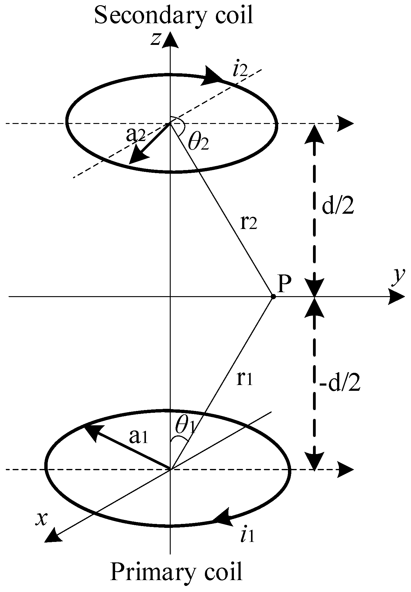
Two single turn loop coils are set up as coupled coils of an IPT system to realize wireless power transfer by magnetic coupling. Figure 1 shows two adjacent, aligned coils of an IPT system, separated by a distance d. The primary coil with a radius a1 is in the plane z = −d/2 and the secondary coil with a radius a2 is in the plane z = d/2. The primary coil is driven by a high frequency AC current i1, and i2 is the induced current in the secondary coil.
The open circuit voltage and the induced current in the secondary (including the amplitude and the phase ) are listed below, respectively,
where ω is the system running frequency, Z2 is the total impedance of the secondary coil, RL is the uniformly distributed load in the secondary, and M is the mutual inductance between two coupled coils. No compensation circuit is used for two coupled coils. The equivalent series resistors (ESR) of the primary and the secondary coils are ignored. The coil currents are expressed in time domain as, respectively,
where and are the amplitude values of currents in both the primary and the secondary coil, and φ is the initial phase difference of the secondary current with respect to the primary current.
The electromagnetic fields at an arbitrary point in the space by two coupled coils are expressed, respectively, as [12],
where ri, θi and φ represents the radial distance, the polar angle, and the azimuthal angle in the spherical coordinates, respectively. , and are the orthogonal unit vectors in the directions of ri, θi and φ in the spherical coordinates. The unit vector represents the direction in which the radial distance from the center of two coils increases, represents the direction in which the angle from the positive z-axis is increasing, and represents the direction in which the angle in the xy plane counterclockwise from the positive x-axis is increasing. E1, H1, and E2 and H2 are electromagnetic fields generated by the primary and the secondary coil, respectively, at an arbitrary point P as shown in Figure 1. ω is system angular frequency and k is the wavelength number, defined as k = 2π/λ = ω/c. r1 and r2 are the distances from the center of two coils to the point P, and η is the wave impedance of the free space.
3. Poynting Vector in an IPT System
At an arbitrary point between two coupled coils, the time-averaged Poynting vector S, by its definition as the half of the cross-product of E and conjugate H (H*), is expressed in (5),
The total time-averaged Poynting vector includes the Poynting vector S1 contributed by the primary coil only, S2 solely by the secondary coil, and the cross components S12 and S21 by interaction between the two coils.
where in (7).
Equation (6) shows the S1 and S2 have components in r direction only. Equation (7) shows that both S12 and S21 have two components in the r direction and in the θ direction, respectively. As aforementioned, the majority of IPT system running frequencies range from tens of kHz [1,4,13] up to 13.56 MHz [14,15,16], so the wavelength number k (k = ω/c) is much less than 1 with the decrease of operating frequency of the system.
In terms of the transferred power from the primary coil to the secondary coil in an IPT system, S1 and S2 are contributed by Poynting vectors that are generated by the primary coil and the secondary coil separately, whose magnitudes decrease as the fourth power of wavelength number k. S1 and S2 are very small at IPT system frequencies, when compared to the interactive components of S12 and S21, which are directly proportional to k. It is obvious that S1 and S2 do not contribute much to the system power transfer, when compared to two coupling components S12 and S21. This suggests at an arbitrary point near the coupled coils in an IPT system, the coupled parts S12 and S21 dominate the system power transfer, and S1 + S2 in (5) could be neglected. Similarly, high order components (≥2) of k in the expressions of the coupled parts S12 and S21 in (7) are neglected for simple calculation.
The interactive parts of time-averaged Poynting vector at a point in an IPT system is then be simplified, as shown in (8).
where in (8).
Then the interactive components from the spherical coordinate are then transformed to the S in the Cartesian coordinate in (9) for consistency where two coils are located physically for straight forward understanding.
Finally, the simplified Poynting vector S is shown in (10) as a vector with components in x, y, and z directions, respectively, in the Cartesian coordinate.
where in (10).
4. Power Distribution Analysis
4.1. Analytical Analysis
The primary coil is driven by a 10 A (peak value) sinusoidal current source at 1 MHz, and the peak current induced in the secondary coil is 5.6242 A. The phase of the secondary current is 0.2734 rad lagging that of the primary current. The primary coil and the secondary coil have equal radii, a1 = a2 = 0.48 m, and equal wire diameter of 0.01 m. These two coils are separated with a distance of d = 0.4 m. As the Poynting vector is generated three-dimensionally in the space between two coils, the two-dimensional (2D) yz cross-section plane in the Cartesian coordinate is chosen to visualize the Poynting vector for straightforward presentation.
The calculated time-averaged Poynting vectors components Sy and Sz are expressed in (11), where the magnitudes and directions of these two components are closely related to the coordinate of the selected point in the yz plane. As the azimuthal angle φ in the yz plane is π/2, Sy, and Sz in the yz plane from (10) are further simplified as (11),
where .
Figure 2 shows the 2D analytical result of the power distribution results between the two coupled coils. The horizontal axis is the y axis, and the vertical axis is the z-axis. The center (y = 0) of the primary coil and the secondary coil is located co-axially along the z axis, where the radius of each coil is 0.48 m. The primary coil (z = −0.2) is below the secondary (z = 0.2) with a distance d = 0.4 m. The y and z components of the time-averaged Poynting vector field, shown in (11), were visualized by using Mathematica. The directions of the time-averaged Poynting vector fields are shown with arrows and the strength of the vectors are shown with colors. The two points (y = −0.48 and y = 0.48) on the y-axis (horizontal axis) are the edges of the coils and the Poynting vector distributes in a round shape between two coils in the yz plane. The strength of the Poynting vector fields, and thus the power density, decreases as the selected point approaches to the symmetrical axis between the two coils, or moves away from the edges of the two coils. The directions of the Poynting vector fields, and thus the power transfer path, are found to be concentrated at the edges of the coils, as opposed to the center path. The maximum magnitude of the Poynting vector in the yz plane is around 0.4 VA/m2, according to the result.
4.2. Numercial Analysis
This section shows the power density distribution simulation results of the proposed IPT system by using the electromagnetic studio (EMS) of computer simulation technology (CST) software package. CST EMS was used to setup the parameters of the coupled coils for power distribution analysis. It is a dedicated software package which can be used for studying the current flow, magnetic and electric field distribution, dynamic power flow, and other static to medium frequency variables of electromagnetic systems. The coil parameters of the system setup are kept the same as before for consistency with the analytical analysis. The same 2D cross-section plane yz is also used to show the Poynting vector distribution in the Cartesian coordinate.
Figure 3 shows 2D simulation result of the power distribution in the yz plane between the primary and the secondary coils from CST. The primary coil is located axially below the secondary coil. The directions of arrows show the directions of Poynting vector fields pointing to and the colors of them present the amplitudes of Poynting vector. The distribution results show that power is transferred from the primary to the secondary coil concentrates along the edges of two coils. Away from the coil edges or along the center path, the strength of Poynting vector fields decrease. The power distributes in a round shape at the edges of two coils in the yz plane.
It can be seen from Figure 2 and Figure 3 that most Poynting vectors between the coupled coils point from the primary coil to the secondary coil. It also shows most power distributes between the two edges of coils instead of focusing along the center axis. As the system is symmetrical, in a three-dimensional (3D) domain, the power density distribution would be in a donut shape between and along the perimeter of the two coils. The magnitudes, directions, and distribution of the Poynting vectors of shown in Figure 2 and Figure 3 are in good agreement. Figure 2 shows the maximum values of the Poynting vector fields are around 0.4 VA/m2, according to the results and Figure 3 shows almost the same amplitudes of the time-averaged Poynting vector, which validates the correctness of the proposed analytical Poynting vector model.
5. Power Flow Analysis
5.1. Power Transfer across Mid-Plane from Primary Coil to Secodnary Coil
The power distribution and transfer path have been determined by analytical analysis and numerical analysis in the last section, and this section presents a further quantitative analysis of power flow. Figure 4 shows the Poynting vector distribution sketch in the xy mid-plane. The Poynting vector at any point has components in x, y, and z directions. Power is transferred from the primary coil to the secondary coil along the z direction, the Poynting vector components in x and y directions do not contribute to system power transfer as the power transfers along the z axis.
From Figure 4, the selected point P is in the xy plane along the y axis, and r is the distance between P and the origin, which indicates the radius of the mid-plane. Then, the coordinate transformation from the spherical coordinate to the Cartesian coordinate is given by (12).
The Poynting vector in the xy plane could be simplified as (13) by substituting all of the known parameters in (12) to (10),
The total Poynting vector includes the z component in the central cross-section plane (xy plane) only, and the x and y component of Poynting vectors are calculated as 0. Then, integrate the z component on the infinite cross-section plane to derive the average power transfer across the mid-plane between two coupled coils,
where kη = ωµ0, µ0 and ε0 are the magnetic permeability and electric permeability in vacuum. (14) is further simplified as,
where ω is system working frequency.
I1 and I2 are RMS values of the currents in both the primary and secondary coil, ϕ is the phase of the secondary current lagging that of the primary current.
Equation (15) shows the surface integral of the perpendicular Poynting vector components is equal to the power transferred from the primary to the secondary. The power transferred across the mid-plane is determined by the system frequency, the radii of the primary and the secondary, the RMS values of two coil currents, the phase between two currents, and the coupling distance. The result is consistent with that from the circuit theory of [18]. Note the xy plane is chosen here as the mid-plane to simplify the calculation, and it is possible to verify that the Poynting vector method in relation to the average power flow applies to any infinite surface perpendicular to the axis between the two coupled coils.
Two extreme conditions, including an open secondary and a shorted secondary, are considered to prove the validity of the Poynting vector in an IPT system. An IPT system is running with the primary driven by a sinusoidal current and the secondary coil is open circuited, so there is an induced voltage across the secondary coil with no current. The Poynting vectors contributed by the secondary coils are zero and the total Poynting vector is simplified as S1. The time-averaged Poynting vector that is generated by the primary coil, is,
The total time-averaged Poynting vector S is equal to 0 as the z component of the Poynting vector is 0 in (17), when the secondary is open. No real power is transferred to the secondary coil, which matches the result from the circuit theory.
Then, the IPT system is running when the primary is driven by a sinusoidal current and the secondary coil shorted. There is an induced voltage across the secondary coil and an induced short current in the secondary coil. The total Poytning vector from (5) is expressed as,
By the coordinate transformation in (12), the Poynting vector is derived as the following form, including only the z component,
is the amplitude value of short current in the secondary coil, and the transferred power is determined by the z component of the total Poynting vector S in (19). The time-averaged Poynting vector is direct proportional to sin ϕ, and ϕ is the phase difference between the secondary current and the primary current. According to Lenz’s law, the induced current in the secondary is in phase with the primary current if the secondary coil is shorted. Consequently, as the term sin ϕ is 0 when the secondary coil is shorted, and this means that no real power flows to a shorted secondary IPT system.
5.2. Example Power Flow Analysis
Table 1 shows the parameters of an example IPT setup for analyzing the power flow between the two coupled coils. These parameters are kept the same for both analytical and numerical analyses. The IPT system operating frequency f is set at 1 MHz so the system angular frequency ω is 6.2832 × 10⁶ rad/s, accordingly. The primary coil is driven by a 10 A (peak value) sinusoidal current source and the secondary coil is assumed to have a uniformly distributed load RL 5 Ω. The primary and the secondary coils have identical geometries, with equal radius a1 and a2 of 0.48 m, and equal wire radius b1 and b2 of 0.005 m. The separate distance d between the primary and the secondary coil is 0.4 m, with the coils aligning along the z-axis at z = +0.2 m and −0.2 m, respectively.
With the parameters given in Table 1, the self-inductance of each circular loop coil can be calculated [19,20] as,
where a is the radius of the coils, and b is the wire radius. Note both a and b should be calculated in inches in (20), which is different from the units shown in Table 1.
The mutual inductance [5,6,17] can also be calculated by (21), which is determined by the radius of two coils and separation distance,
Then, the induced peak current in the secondary coil can be obtained based on the coupled circuit theory,
Now, the input and output power can be calculated. Because the IPT system is assumed to be lossless without considering the ESRs of the primary and the secondary coils, and the power loss in the air is negligible, it is reasonable to predict that the input power to the primary coil Pin is equal to the output power to the secondary coil Pout, which is verified by the following analysis.
The input power Pin provided by the primary coil can be calculated by the reflected impedance from the secondary coil, which is determined by the RMS value of the current in the primary and the real part of the reflected impedance from the secondary. It is calculated as,
Similarly, the output power Pout received by the load is calculated by the coupled circuit theory, which is related to the RMS value of the induced current and load value in the secondary coil,
As expected, these two results are in good agreement from (23) and (24). The previous analyses are based on lumped circuit models.
The power flow across a mid-plane can be calculated by the power distribution described by the Poynting vector analysis in Section 5.1. In the example system setup with parameters shown in Table 1, the power flow across the mid-plane (which equals to the integral of the z component of the Poynting vector over the infinite surface xy plane) can be calculated as,
where µ0 is the magnetic permeability in vacuum (µ0 = 4π × 10−7 H·m−1), and ϕ is the phase of the secondary current lagging that of the primary current (sin ϕ = 0.2734).
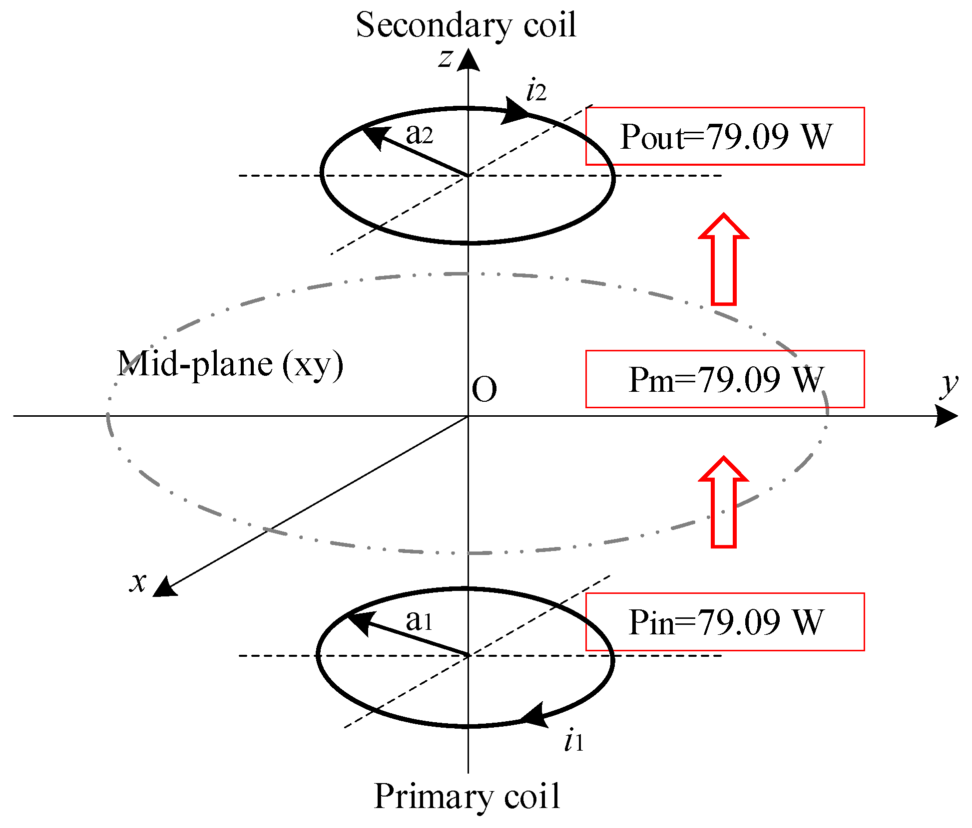
These results show the power transfer across the mid plane Pm is equal to the input and output power calculated in (23)–(25). Figure 5 illustrates that the power flow from the primary coil to the secondary via the mid plane (power transfer direction is shown with red arrows) in the example two-coil IPT system, which verifies that the Poynting vector method is valid to analyze the power flow and power distribution between the coils. The general power results at the input and output ends are consistent with the lumped circuit theories, but the proposed Poynting vector approach can be used for power flow and distribution in the medium between two coupled coils in an IPT system.
6. Conclusions
This paper has analyzed the power distribution and power flow between two coupled coils of an IPT system by using the Poynting vector. A two-coil setup of an IPT system has been modelled with the primary coil driven by a current source, and a uniformly loaded secondary. Then, the Poynting vector at an arbitrary point is analyzed by calculating the magnetic and electric fields between the two coils. Analytical results and numerical results of the power distribution from Mathematica and CST has been obtained and compared, and the result shows that the power distributes as a donut shape in 3D space and concentrates along the edges of two coils in the proposed setup, as opposite to the central path. Additionally, quantitative power flow analysis across a mid-plane between the two coils has been conducted with an infinite mid-plane surface integral of the Poynting vector, which has been compared with the input and the output power from the primary and the secondary coil. The results show that power across the mid-plane, the input power of the primary, and the output power to the secondary are in good agreement, which verifies the Poynting vector method, and demonstrates the power flow from the primary to the secondary coil. The proposed Poynting vector method provides an effective approach to analyze the power flow and distribution between two coupled coils in a near field IPT system, which cannot be achieved by traditional lumped circuit theories.
Acknowledgments
The authors would like to express their gratitude to the Department of Electrical and Computer Engineering of the University of Auckland, as well as PowerbyProxy (Apple) for their financial and technical supports.
Author Contributions
Both authors have contributed to this work. Yuan Liu is the corresponding author of this manuscript and contributed to the theoretical analysis, modeling, simulation, and draft preparation. Aiguo Patrick Hu provided general guidance for this research work and supervised the whole project.
Conflicts of Interest
The authors declare no conflict of interest.
References
- Green, A.W.; Boys, J.T. 10 kHz inductively coupled power transfer-concept and control. In Proceedings of the Fifth International Conference on Power Electronics and Variable-Speed Drives, London, UK, 26–28 October 1994; pp. 694–699. [Google Scholar]
- Hu, A.P. Selected Resonant Converters for IPT Power Supplies. Ph.D. Thesis, University of Auckland, Auckland, New Zealand, 2001. [Google Scholar]
- Wang, C.-S. Design Considerations for Inductively Coupled Power Transfer Systems; Electrical and Electronic Engineering—University of Auckland: Auckland, New Zealand, 2004. [Google Scholar]
- Madawala, U.K.; Thrimawithana, D.J. A bidirectional inductive power interface for electric vehicles in V2G systems. IEEE Trans. Ind. Electron. 2011, 58, 4789–4796. [Google Scholar] [CrossRef]
- Kurs, A.; Karalis, A.; Moffatt, R.; Joannopoulos, J.D.; Fisher, P.; Soljacic, M. Wireless power transfer via strongly coupled magnetic resonances. Science 2007, 317, 83–86. [Google Scholar] [CrossRef] [PubMed]
- Karalis, A.; Joannopoulos, J.D.; Soljačić, M. Efficient wireless non-radiative mid-range energy transfer. Ann. Phys. 2008, 323, 34–48. [Google Scholar] [CrossRef]
- Cheon, S.; Kim, Y.H.; Kang, S.Y.; Lee, M.L.; Lee, J.M.; Zyung, T. Circuit-Model-Based Analysis of a Wireless Energy-Transfer System via Coupled Magnetic Resonances. IEEE Trans. Ind. Electron. 2011, 58, 2906–2914. [Google Scholar] [CrossRef]
- Kiani, M.; Ghovanloo, M. The Circuit Theory behind Coupled-Mode Magnetic Resonance-Based Wireless Power Transmission. IEEE Trans. Circuits Syst. I Regul. Pap. 2012, 59, 2065–2074. [Google Scholar] [CrossRef] [PubMed]
- Fan, J.; Yu, F.; Zhang, G.; Tian, Z.; Liu, J. Two Fundamental Physics Issues Need Paying Great Attention in Wireless Power Transmission. Trans. China Electrotech. Soc. 2013, 28, 61–65. [Google Scholar]
- Faria, J.B. Poynting vector flow analysis for contactless energy transfer in magnetic systems. IEEE Trans. Power Electron. 2012, 27, 4292–4300. [Google Scholar] [CrossRef]
- Guo, Y.; Li, J.; Hou, X.; Lv, X.; Liang, H.; Zhou, J.; Wu, H. Poynting vector analysis for wireless power transfer between magnetically coupled coils with different loads. Sci. Rep. 2017, 7, 741. [Google Scholar] [CrossRef] [PubMed]
- Li, L.-W.; Leong, M.-S.; Kooi, P.-S.; Yeo, T.-S. Exact solutions of electromagnetic fields in both near and far zones radiated by thin circular-loop antennas: A general representation. IEEE Trans. Antennas Propag. 1997, 45, 1741–1748. [Google Scholar]
- Boys, J.T.; Covic, G.A.; Green, A.W. Stability and control of inductively coupled power transfer systems. IEE Proc. Electr. Power Appl. 2000, 147, 37–43. [Google Scholar] [CrossRef]
- Chen, W.; Chinga, R.; Yoshida, S.; Lin, J.; Chen, C.; Lo, W. A 25.6 W 13.56 MHz wireless power transfer system with a 94% efficiency GaN class-E power amplifier. In Proceedings of the 2012 IEEE MTT-S International Microwave Symposium Digest (MTT), Montreal, QC, Canada, 17–22 June 2012; pp. 1–3. [Google Scholar]
- Fu, M.; Zhang, T.; Zhu, X.; Ma, C. A 13.56 MHz wireless power transfer system without impedance matching networks. In Proceedings of the 2013 IEEE Wireless Power Transfer (WPT), Perugia, Italy, 15–16 May 2013; pp. 222–225. [Google Scholar]
- Li, X.; Tsui, C.Y.; Ki, W.H. A 13.56 MHz Wireless Power Transfer System with Reconfigurable Resonant Regulating Rectifier and Wireless Power Control for Implantable Medical Devices. IEEE J. Solid-State Circuits 2015, 50, 978–989. [Google Scholar] [CrossRef]
- Jackson, J.D. Classical Electrodynamics; Wiley: Hoboken, NJ, USA, 1999. [Google Scholar]
- Li, S.; Mi, C.C. Wireless Power Transfer for Electric Vehicle Applications. IEEE J. Emerg. Sel. Top. Power Electron. 2015, 3, 4–17. [Google Scholar]
- Grover, F.W. Inductance Calculations: Working Formulas and Tables; Courier Corporation: North Chelmsford, NA, USA, 2004. [Google Scholar]
- Terman, F.E. Radio Engineers’ Handbook; McGRAW-Hill Book Company, Inc.: New York, NY, USA; London, UK, 1943. [Google Scholar]
Figure 1.
Primary coil and secondary coil setup of an inductive power transfer (IPT) system.

Figure 2.
Two-dimensional (2D) analytical result of the power distribution between the primary and secondary coil using Mathematica.
Figure 2.
Two-dimensional (2D) analytical result of the power distribution between the primary and secondary coil using Mathematica.
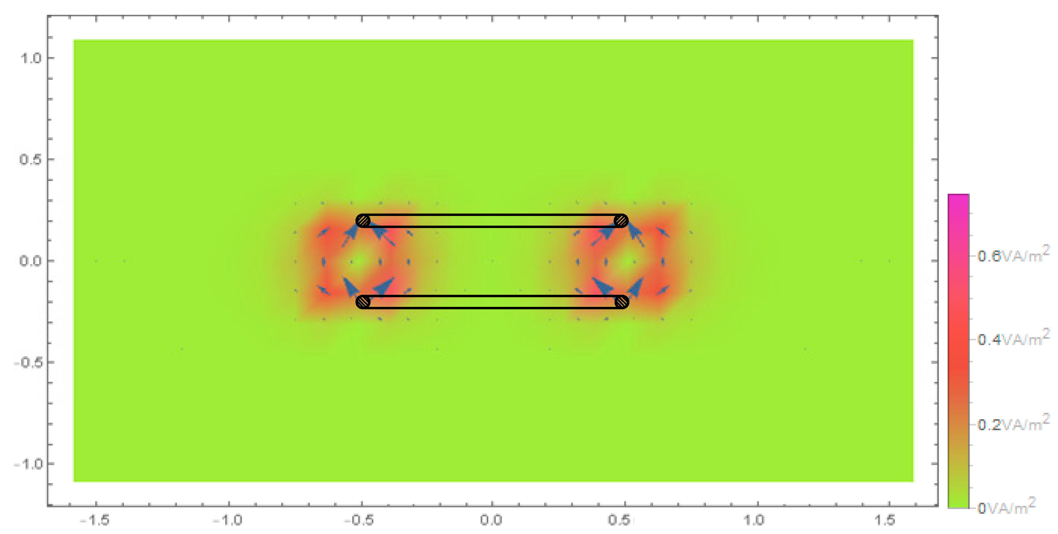
Figure 3.
2D simulation result of the power distribution between the primary and secondary coil using computer simulation technology (CST).
Figure 3.
2D simulation result of the power distribution between the primary and secondary coil using computer simulation technology (CST).
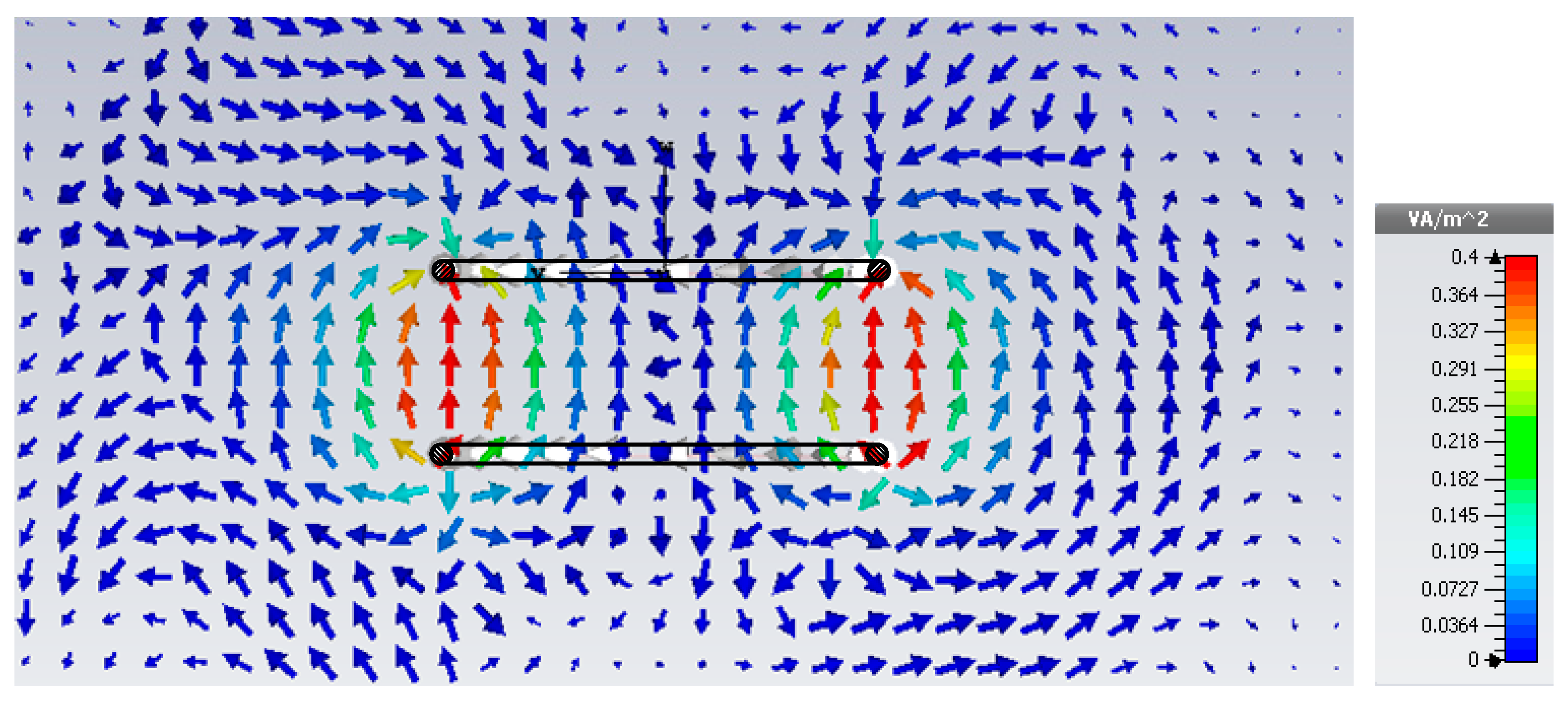
Figure 4.
Poynting vector distribution sketch in the xy mid-plane.
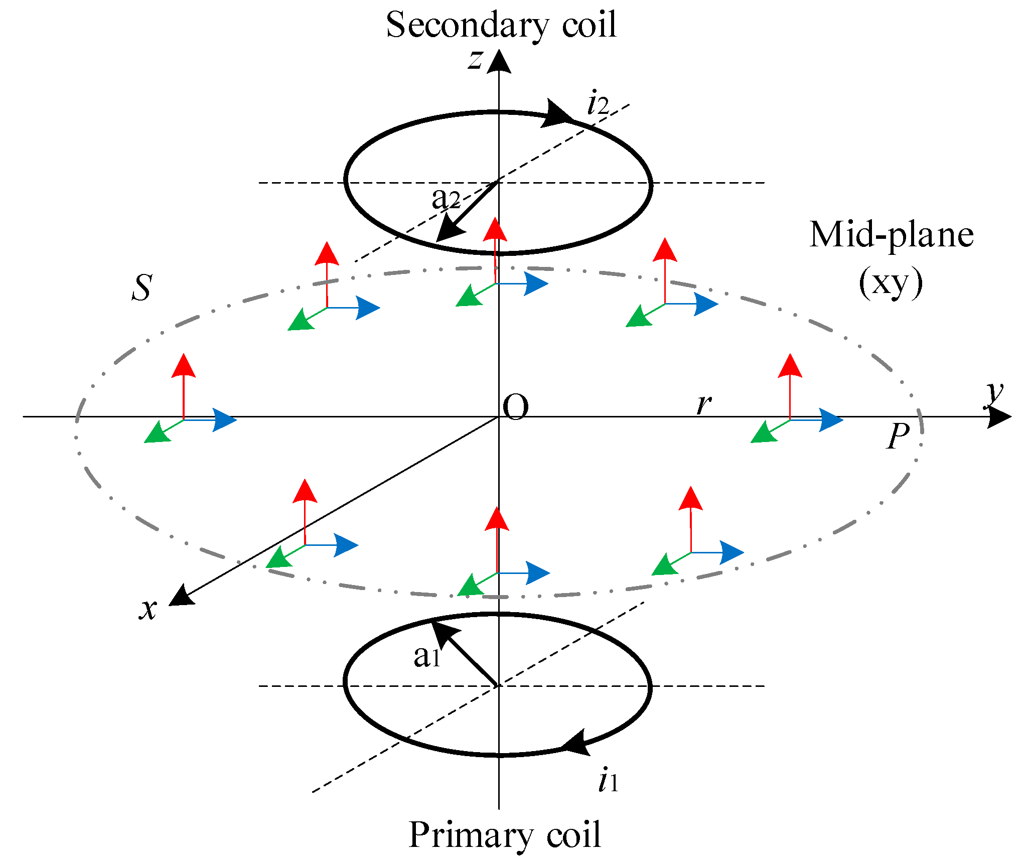
Figure 5.
Input power, power across the mid-plane and output power of the example two-coil IPT system.
Figure 5.
Input power, power across the mid-plane and output power of the example two-coil IPT system.

Table 1.
Parameters of an example IPT setup.
| Parameters | Values | Parameters | Values |
|---|---|---|---|
| f | 1 MHz | a1 = a2 | 0.48 m |
| ω | 6.2832 × 10⁶ rad/s | b1 = b2 | 0.005 m |
| 10 A | d | 0.4 m | |
| N1 = N2 | 1 | RL | 5 Ω |
© 2018 by the authors. Licensee MDPI, Basel, Switzerland. This article is an open access article distributed under the terms and conditions of the Creative Commons Attribution (CC BY) license (http://creativecommons.org/licenses/by/4.0/).
Share and Cite
MDPI and ACS Style
Liu, Y.; Hu, A.P. Study of Power Flow in an IPT System Based on Poynting Vector Analysis. Energies 2018, 11, 165. https://doi.org/10.3390/en11010165
AMA Style
Liu Y, Hu AP. Study of Power Flow in an IPT System Based on Poynting Vector Analysis. Energies. 2018; 11(1):165. https://doi.org/10.3390/en11010165
Chicago/Turabian StyleLiu, Yuan, and Aiguo Patrick Hu. 2018. "Study of Power Flow in an IPT System Based on Poynting Vector Analysis" Energies 11, no. 1: 165. https://doi.org/10.3390/en11010165
Note that from the first issue of 2016, this journal uses article numbers instead of page numbers. See further details here.