A Novel Algorithm for Optimal Operation of Hydrothermal Power Systems under Considering the Constraints in Transmission Networks

Abstract

This paper proposes an effective novel cuckoo search algorithm (ENCSA) in order to enhance the operation capacity of hydrothermal power systems, considering the constraints in the transmission network, and especially to overcome optimal power flow (OPF) problems. This proposed algorithm is developed on the basis of the conventional cuckoo search algorithm (CSA) by two modified techniques: the first is the self-adaptive technique for generating the second new solutions via discovery of alien eggs, and the second is the high-quality solutions based on a selection technique to keep the best solutions among all new and old solutions. These techniques are able to expand the search zone to overcome the local optimum trap and are able to improve the optimal solution quality and convergence speed as well. Therefore, the proposed method has significant impacts on the searching performances. The efficacy of the proposed method is investigated and verified using IEEE 30 and 118 buses systems via numerical simulation. The obtained results are compared with the conventional cuckoo search algorithm (CCSA) and the modified cuckoo search algorithm (MCSA). As a result, the proposed method can overcome the OPF of hydrothermal power systems better than the conventional ones in terms of the optimal solution quality, convergence speed, and high success rate.

1. Introduction

Optimal power flow (OPF) is a complex problem for the operation of a power system due to its dependence on many equality and inequality constraints, such as the limit of active and reactive powers of electric generators, transformer tap positions, switchable capacitor banks, bus-voltage values, and capacity of lines transmission [1]. The purpose of the OPF problem is to determine the values of control variables and how to carry out an OPF in order to obtain all dependent variables. A solution is considered an optimal result if it gives the minimum fuel cost for all thermal units while satisfying all dependent variables and constraints. Normally, the OPF problem is only run for one sub-interval.

The hydrothermal scheduling (HTS) problem is relatively different from the OPF problem since the thermal and hydro units are included in power systems. The target of the HTS problem is to minimize the fuel cost of the thermal units in various scheduled sub-intervals while satisfying all constraints in the generators’ capacities, the balance of power systems, as well as limitations of water discharge, water balance, etc. In addition, the optimal operation of hydrothermal systems is divided into many sub-intervals, which is more complicated than a single sub-interval in the OPF problem. Apparently, the OPF problem considers all constraints in transmission lines, but hydraulic constraints from hydropower plants are neglected.

Practically, so far the HTS and OPF problems have been studied independently. For instance, the HTS problem was discussed in [1,2,3,4,5,6,7,8,9,10,11,12] and the OPF problem was presented in [13,14,15,16,17,18,19,20,21,22,23,24,25,26,27,28,29,30,31,32,33,34,35,36,37,38,39,40,41,42,43,44,45,46,47]. However, combining the OPF and HTS problems was attempted by the authors in [48,49,50,51,52,53,54]; but they only use methods belonging to the deterministic algorithms [48,49,50,51,52,53] applied in the past three decades. In order to solve this combined problem, Newton’s is the first method applied, where IEEE systems from 5 to 118 buses accompanied by a fixed-head short-term hydropower plant model are tested. The study objective is only to indicate the ability of the Newton approach to deal with the complicated problem and to satisfy all constraints such as the voltage, generation limitations on units, as well as other constraints in transmission lines. The whole data of the test systems was not given in these papers and the objective function values were not considered for comparisons. The two difficulties have restricted to attract attention from researchers, leading to a small number of published papers regarding the problem. In [49,50,51,52], the authors only considered the transmission network constraints when dealing with the hydrothermal system scheduling problem. They have built and solved their own problem data and their applied method could handle the problem. On the contrary, in [53], the authors have proposed an improved particle swarm optimization (PSO) algorithm to solve the eight-bus system; as in previous studies, the improved PSO is used in order to obtain the optimal solution for the HTS problem while satisfying the constraints of the OPF problem. The authors of [54] have developed a conventional cuckoo search algorithm (CCSA) for solving the hydrothermal optimal power flow problem (HTOPF) and the performance of the conventional CSA was also compared via conventional PSO. They supposed that the capacitor bank and tap changer were the continuous variables and the load demands between different subintervals were identical to the given data in the OPF problem. This assumption could help verify the effectiveness and robustness of conventional CSA compared to the conventional PSO. However, the capacitors and tap should be the discrete variables in practice and the load demands of different subintervals should be different. Consequently, in order to solve the hydrothermal OPF problem, this paper proposes an effective novel cuckoo search algorithm (ENCSA) for optimizing the operation of hydrothermal power systems, taking into account all constraints belonging to the transmission power networks and considering the minimization of electricity and fuel costs as the objective function. The procedure for searching CCSA [55] is constructed of five main steps: step 1, the first update of new solutions via the theory of Lévy flights; step 2, comparison and selection; step 3, the second update of new solutions via a mutation operation; step 4, comparison and selection; and step 5, the determination of the best solution. Modified CSA (MCSA) [56] has focused on the improvement in the first update of new solutions using Lévy flights, while the next four steps have remained unchanged in MCSA. This MCSA has divided all current solutions into two subgroups by quality, in which the first one contains lower fitness function solutions and the second one contains higher fitness function solutions. Each solution in the first subgroup is newly produced by using its old solution and two other ones in the group, while each solution in the second subgroup is newly updated as in step 1 of CCSA, i.e., using an old solution and the best solution. In addition, MCSA has suggested an adaptive value for the scaling factor, with the change depending on the iteration. In ENCSA, we focus on improvement of steps 3 and 4, corresponding to the second update of new solutions and the comparison and selection. In the second update of new solutions, we propose an adaptive mutation technique by using two mutation modes simultaneously for current solutions. Solutions far away from the so-far best solution will use a jumping step with two random solutions and they are newly updated. On the contrary, solutions close to the so-far best solution will use four random solutions to produce a jumping step and solutions are sought around the so-far best solution instead of around the current solution. In step 4, CCSA makes a comparison between each old solution and each new solution at the same nest and keeps the better one. The selection can cope with a mistake (i.e., a better solution at one nest can be worse in quality than another one at other ones). For this case, CCSA omitted promising solutions. Thus, we have tackled the cons of CCSA by suggesting a second modification: firstly, all old solutions and all new solutions are mixed together; secondly, identical solutions are identified, and only one solution is retained, while others are eliminated; finally, a set of the best solutions is stored for the next step of determining the best solution. To investigate the improvement of ENCSA over CCSA and MCSA, we perform simulation experiments on IEEE 30 and 118 buses systems. The obtained results are analyzed and compared to those from CCSA and MCSA. More concretely, the main contribution includes the following aspects:

(i)

Successfully improve the optimal solution search ability of ENCSA;

(ii)

Successfully formulate a hydrothermal power system scheduling problem considering all constraints in transmission power networks;

(iii)

Successfully deal with all constraints such that they can be satisfied completely thanks to the appropriate selection of decision variables.

This paper is divided into one appendix and six sections. Starting with an introduction in Section 1, Section 2 covers the formulation of the hydrothermal optimal power flow problem while Section 3 gives the proposed algorithm for optimal power flow problem of the hydrothermal power systems. Section 4 presents an application of the proposed method to deal with the optimal power flow problems, while simulation results are handled in Section 5 and Appendix A. Finally, conclusions are reported in Section 6.

2. Hydrothermal Optimal Power Flow Problem Formulation

The main formulation for dealing with the optimal power flow problems of hydrothermal power systems is as follows.

2.1. Fuel Cost Objective

The objective optimization of the considered problem is to reduce the total electricity generation and fuel costs of all available generating units as [3]:

$$\mathrm{Min} {\displaystyle \sum _{\mathrm{i}=1}^{N_g}{F}_i(P_{gi})},$$

(1)

where F_i(P_gi) is the electricity generation cost of the ith generating thermal unit and can be described by the following second-order equation:

$$F_i(P_{gi})=a_i+b_i{P}_{gi}+c_i{P}_{gi}^2.$$

(2)

2.2. Hydrothermal System Constraints

Water availability constraints can be described as follows [4]:

$${\displaystyle \sum _{m=1}^M{t}_m{q}_{j,m}}=W_j;j=1,\dots ,N_2,$$

(3)

where q_j,m is the water discharge via hydro turbine j in subinterval m and can be calculated by:

$$q_{j,m}=a_{hj}+b_{hj}{P}_{hj,m}+c_j{P}_{hj,m}^2.$$

(4)

Generator Operating Limits: The active and reactive powers of thermal and hydro units are constrained between their minimum and maximum values as follows:

$$\begin{array}{l}{P}_{gi,\min }\le P_{gi}\le P_{gi,\max };i=1,\dots ,N_g,\\ Q_{gi,\min }\le Q_{gi}\le Q_{gi,\max }; i=1,\dots ,N_g\end{array}.$$

(5)

Generation bus voltage limits: The operating voltage of all generators is constrained within their boundaries:

$$V_{gi,\min }\le V_{gi}\le V_{gi,\max }; i=1,\dots ,N_g.$$

(6)

2.3. Transmission Network Constraints

Power balance: The active and reactive power balance between the load and generator at each bus is considered [13]:

$$\begin{array}{l}{P}_{gi}-P_{di}=V_i{\displaystyle \sum _{j=1}^{N_b}{V}_j\left[G_{ij}\cos ({\delta }_i-{\delta }_j)+B_{ij}\sin ({\delta }_i-{\delta }_j)\right]}; i=1,\dots ,N_b,\\ Q_{gi}+Q_{ci}-Q_{di}=V_i{\displaystyle \sum _{j=1}^{N_b}{V}_j\left[G_{ij}\sin ({\delta }_i-{\delta }_j)-B_{ij}\cos ({\delta }_i-{\delta }_j)\right]}; i=1,\dots ,N_b\end{array}.$$

(7)

Minimum and maximum limits of shunt compensators: The reactive power generated for the grid by capacitor banks must be within the following limitations:

$$Q_{ci,\min }\le Q_{ci}\le Q_{ci,\max }; i=1,\dots ,N_c.$$

(8)

Practically, the reactive power generated for the grid by the capacitor banks is not a continuous variable but a discrete variable. Therefore, the exact value of the capacitor banks should follow the equation [46]:

$$Q_{ci}=Q_{ci,\min }+N_{ci}·\Delta Q_{ci},$$

(9)

where ∆Q_ci is the rated power of each capacitor and N_ci is the selected number of capacitors among the set of available capacitors. However, in some cases, the number of available capacitors and the rated power are not given and only the minimum and the maximum values are given; the value Q_ci is newly generated within its boundaries and then is rounded up or down to the nearest unit.

Limits of transformer tap selection: The selection of transformer taps with aim to stabilize power network voltage but it should be one of a set of specific values of each available transformer at buses by the model below:

$$T_{k,\min }\le T_k\le T_{k,\max }; k=1,\dots ,N_t.$$

(10)

Similar to the capacitor banks variable, the magnitude of the load tap changer is also not a continuous variable but a discrete variable since the tap is changing by a certain increment. This increment is also dependent on the size of the specified transformer, as in the following equation [46]:

$$T_k=T_{k,\min }+N_{tk}·\Delta T_k.$$

(11)

Limitations of voltage at load buses: The operating voltage of each load must be within valid range and can be described as follows:

$$V_{li,\min }\le V_{li}\le V_{li,\max }; i=1,\dots ,N_d.$$

(12)

Limitations of transmission lines: The apparent power flow in each line must be lower than the allowable capacity of conductor, and can be calculated as follows:

$$S_l\le S_{l,\max }; l=1,\dots ,N_l,$$

(13)

where $S_l=\max \left\{\right|S_{ij}|,|S_{ji}\left|\right\}$.

2.4. Control and Dependent Variables

The sets of control and dependent variables of the HTOPF problem are shown in Equations (14) and (15). It is clear that the control variables consist of active power of all generators at all buses except at the slack bus, the voltage of all generators, the transformer tap, and the reactive power of shunt capacitors. The control variables will be added into the program of power flow and then we will obtain the dependent variables given in Equation (15). When all dependent variables can satisfy their boundaries and the objective function can be minimized, the search process is terminated.

$$u=\{P_{g2}, \dots , P_{g{N}_g}, V_{g1}, \dots , V_{g{N}_g}, T_1, \dots , T_{N_t}, Q_{c1}, \dots , Q_{c{N}_c}\}{ }^T,$$

(14)

$$x=\{P_{g1}, Q_{g1}, \dots , Q_{g{N}_g}, V_{l1}, \dots , V_{l{N}_d}, S_{l1}, \dots , S_{l{N}_l}\}{ }^T.$$

(15)

3. The Proposed Algorithm for the Optimal Power Flow Problem of the Hydrothermal Power Systems

This paper develops an improved version of CCSA by carrying out modifications on two existing techniques of CCSA. For the sake of simplicity, the construction of the CCSA is first described in detail as follows.

3.1. Conventional Cuckoo Search Algorithm

The CCSA method is constructed of two random walks and one selection operation. The three phases can be described as follows.

Lévy flights random walk: CCSA utilizes the random walk technique based on the behavior of Lévy flight to produce the first update of new solutions to its search procedure. For solution d, its new solution $X_d^{new}$ is updated by using a jumping step to a nearby old solution X_d. The jumping step is created using the so-far best solution G_best, old solution X_d and Lévy flights random walk, as seen in Equation (16):

$$X_d^{new}=X_d+{\mathsf{\alpha }}_0\left(X_d-G_{best}\right)\mathrm{L}\mathsf{é}\mathrm{vy}(\mathsf{\beta }).$$

(16)

Selective random walk: The selective random walk also plays a role similar to the mutation operation of DE to perform the second update of new solutions for CCSA. A probability of solution replacement P_ro with the range of [0, 1] is selected to balance the old and new solutions effectively. The selective random walk can be employed as in the following model:

$$X_d^{new}=\{\begin{array}{ll}{X}_d+rand.(X_{randper1}-X_{ranper2})& if ran{d}_d < P_{ro}\\ X_d& otherwise\end{array}.$$

(17)

Selection Operation: CCSA utilizes selection operation to perform a comparison between each old solution and each new solution at each nest and retain more promising solutions to avoid accepting worse quality solutions. The selection is based on fitness comparison, as seen in Equation (18):

$$X_d^{}=\{\begin{array}{ll}{X}_d^{new}& if Fitness (X_d^{new})< Fitness(X_d)\\ X_d& otherwise\end{array}, d=1,...., N_p.$$

(18)

The model in Equation (18) is applied twice: first after Lévy flights random walk, and a second time after selected random walk. However, the task of determining the best solution G_best is carried out only one time at each iteration because the best solution will be used in Equation (16) at the beginning of each iteration.

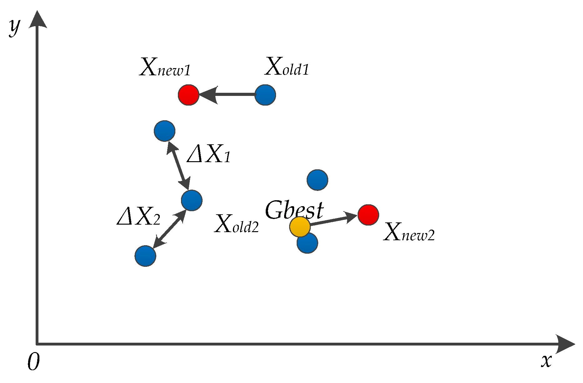
3.2. Proposed Cuckoo Search Algorithm

As described in Section 3.1, CCSA is comprised of three stages including two new solution generations via Lévy flights and discovery of alien eggs, and selection operation. Between the two ways for searching new solutions, the Lévy flight technique focuses on global search while discovery of alien eggs aims to exploit a local search. Moreover, selection operation will be carried out to retain a set of so-far dominant solutions. However, the results obtained from applications of the CCSA to different optimization problems in different fields have indicated that the method has many weak points such as lower-quality solutions, a slow convergence speed, and a high number of iterations. In this paper, an effective novel cuckoo search algorithm (ENCSA) is introduced to tackle the drawbacks of CCSA by constructing two modifications on CCSA. The first modification aims to determine a feasible local search zone for each solution via the discovery of alien eggs while the second modification on selection operation will enable ENCSA to select the potential solutions. The details of the improvements are as follows.

The proposed self-adaptive technique for the second update of new solutions: In the second update of new solutions via selective random walk, CCSA employs two arbitrary solutions to produce a jumping step away from the old solutions for updating a new solution, as shown in Equation (17). However, the impact of this step will be smaller and narrower since the distribution of solutions tends to be close together and the zone near the best solution is ignored when the search process goes to higher iterations. Furthermore, the last iterations are the improvement of solutions near the current best solution because these solutions tend to update their position near the best solution, while searching around the best solution is performed only one time, as the old solution is also the best solution. This issue can lead to a local optimum and low convergence to the highest optimal solution. The restrictions of CCSA can be overcome by employing the search strategy included in Equations (19) and (20):

$$X_d^{new}=X_d+rand.(X_{randper1}^{}-X_{ranper2}^{}) ,$$

(19)

$$X_d^{new}=Gbest+rand.(X_{randper1}^{}-X_{ranper2}^{}+X_{randper3}^{}-X_{ranper4}^{}) .$$

(20)

Obviously, the search methods using the models in Equations (19) and (20) are completely different because the method of Equation (19) is to exploit a small zone around individuals while the aim of applying Equation (20) is to reach the zone around the best solution. Thus, using Equation (20) can produce a jump large enough in the search zone to avoid a local optimum and a fall into a zone very close to the so-far best solution G_best or even at the same position of the best solution. For a better understanding, the assumptions are illustrated in Figure 1, in which X_old2 is much closer to G_best than X_old1, and thus Equation (19) is more appropriate for X_old1 and Equation (20) is better for the case of X_old2. Consequently, using such two models simultaneously for the most effective impact is important to determine an exact criterion. The criterion of small or high distance can be measured mathematically using the fitness function value of each individual and of the best solution, as shown in the model below:

$$D_d=\frac{Fitnes{s}_d-Fitnes{s}_{best}}{Fitnes{s}_{best}}.$$

(21)

Equations (19) or (20) compare D_d and a predetermined tolerance (tol). If D_d is higher than tol, it means the current solution d is far from the best one; Equation (19) should be used. Otherwise, if D_d is equal to or lower than tol, it means the current solution d is closer to the best solution; Equation (20) should be used instead. In the demonstration of this paper, tol is the tolerance picked from one value in the range of [10⁻⁵–10⁻¹]. The procedure for the self-adaptive technique for the second update of new solutions via the discovery action of alien eggs is proposed in

Table 1. Self-adaptive technique for the second update of new solutions.

if randd < Pro   Calculate Dd     if Dd > tol        $X_d^{new}=X_d+rand.(X_{randper1}^{}-X_{ranper2}^{})$     else        $X_d^{new}=Gbest+rand.(X_{randper1}^{}-X_{ranper2}^{}+X_{randper3}^{}-X_{ranper4}^{})$     end   else     $X_d^{new}=X_d$ end

.

The top solutions-based selection technique: As shown in Equation (18), after generating new solutions in the population, at each nest the old solution and its new solution are compared to keep the one with the better fitness function and eliminate the worse one. However, there is no guarantee that all new solutions meet the constraints of the application, thus a retained solution is possibly not the better of the two compared solutions. Additionally, there is a possibility that an abandoned solution at a nest is better than a retained solution at another nest and the selection technique of CCSA could miss some promising solutions to reach the global optimization faster because the current population is not a set of the best candidates. To enhance the alternative technique of CCSA, we propose a new alternative mechanism called the alternative technique-based dominant solution. It is described in

Table 2. The top solutions-based selection technique.

Step 1. Mix all old solutions and all new solutions

Step 2. Identify identical solutions. Keep only one and eliminate rest of identical ones

Step 3. Sort all solutions in order of ascending fitness function values

Step 4. Keep the first Np solutions

.

Applying the proposed high-quality selection technique can retain the best different solutions with lower fitness function and can eliminate worse solutions. In other words, it can keep a set of the best candidates in the population. Therefore, it can support the proposed method converges to global optimal solutions fast and increases the probability of finding solutions meeting all constraints, leading to a high success rate for a number of trial runs.

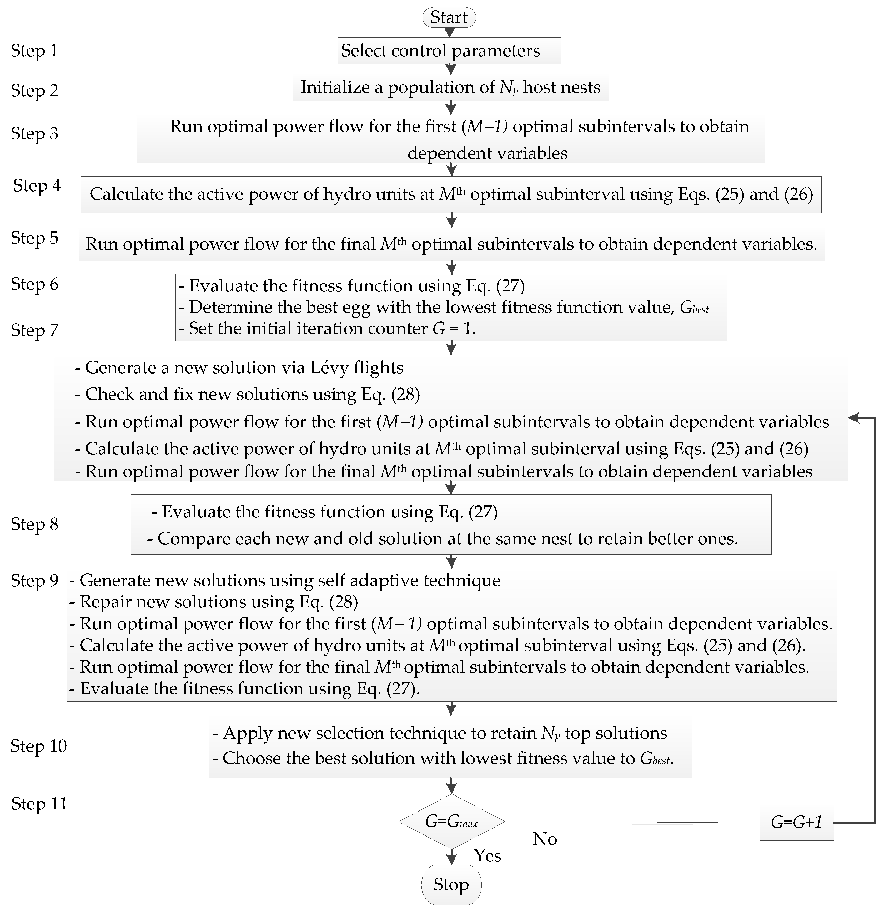
4. Application of the Proposed Method to Deal with the Optimal Power Flow Problems

4.1. Initialization

There are nests N_p in the population of the proposed method and each nest d will contain almost all the control variables in Equation (13). The chosen element in each nest plays a very important role in handling all constraints from hydropower plant reservoirs and transmission lines. Each nest includes all control variables in Equation (13) for M − 1 subintervals, while the output power of all hydropower plants is not included for the last subinterval M. The variables in each nest and the initialization for each nest are as follows:

$$X_{d,m}^{}=[P_{g2}, \dots , P_{g{N}_g}, V_{g1}, \dots , V_{g{N}_g},Q_{c1}, \dots , Q_{c{N}_c}, T_1, \dots , T_{N_t}]; m=1, \dots , M-1,$$

(22)

$$X_{d,m}^{}=[P_{g2}, \dots , P_{g{N}_1}, V_{g1}, \dots , V_{g{N}_g},Q_{c1}, \dots , Q_{c{N}_c}, T_1, \dots , T_{N_t}]; m=M,$$

(23)

$$X_{d,m}^{}=X_{\min }^{}+rand.(X_{\max }^{}-X_{\min }^{}); m=1, 2, \dots , M.$$

(24)

4.2. Calculate the Remaining Control Variables for the Last Subinterval M

All control variables are available for the first M − 1 subintervals, as shown in Equation (22). However, all hydro generations are not given for the last subinterval. Certainly, running power flow will be done only for the first M − 1 subintervals. Consequently, the remaining control variables are found by calculating the water discharges for the first M − 1 subintervals q_j,_m (where j = 1, …, N₂ and m = 1, …, M − 1) for all hydropower plants by substituting generations into Equation (4); then using Equation (3), the water discharges for the last subinterval Mq_j,M are obtained under the conditions of Equation (3), as follows:

$$q_{j,M}=(W_j-{\displaystyle \sum _{m=1}^{M-1}{t}_m{q}_{j,m})/t_M}; j=1,\dots ,N_2.$$

(25)

As a result, all hydro generations during the last subinterval P_hj,M are determined using Equation (4), as follows:

$$P_{hj,M}=\frac{-b_{hj}\pm \sqrt{b_{hj}^2-4c_{hj}(a_{hj}-q_{j,M})}}{2c_{hj}}.$$

(26)

4.3. Calculate Fitness Function

All the control variables are given and the power flow can be run for all M subintervals to obtain dependent variables, as shown in Equation (15). Then, it is necessary to calculate the fitness function for evaluating the solution quality. The fitness function of each solution is a sum of the total electricity generation fuel costs of all generators and the penalty terms for limitation violations of dependent variables. The following equation can enable the calculation of such a fitness function [54]:

$$\begin{array}{ll}FT=& F_1+K_1{\displaystyle \sum _{j=1}^{N_2}{\left(P_{hjM}-P_{hjM}^{\lim }\right)}^2}+K_2{\displaystyle \sum _{m=1}^M{\left(P_{g1,m}-P_{g1,m}^{\lim }\right)}^2}+K_3{\displaystyle \sum _{m=1}^M{\displaystyle \sum _{i=1}^{N_g}{\left(Q_{gi,m}-Q_{gi,m}^{\lim }\right)}^2}}\\ & +K_4{\displaystyle \sum _{m=1}^M{\displaystyle \sum _{i=1}^{N_d}{\left(V_{li}-V_{li}^{\lim }\right)}^2}}+K_5{\displaystyle \sum _{m=1}^M{\displaystyle \sum _{l=1}^{N_l}{\left(S_l-S_l^{\lim }\right)}^2}}\end{array},$$

(27)

where K₁, K₂, K₃, K₄, and K₅ are penalty factors associated with dependent variables.

Before going on to the search procedure of the proposed method, starting with the first update of new solutions, the best solution G_best with the lowest fitness function is determined.

4.4. Handling New Solutions Violating Limitations

Generate new solutions by using Lévy flights, as shown in Equation (16), and using the adaptive selective random walk technique, as shown in Section 3.2; after each generation, all new solutions do not always satisfy their limitations. Thus, they need to be checked and repaired in case of violation, as below:

$$X_{d,m}^{new}=\{\begin{array}{l}{X}_{}^{\max } \mathrm{if} X_{d,m}^{new}> X_{}^{\max } \\ X_{}^{\min } \mathrm{if} X_{d,m}^{new}< X_{}^{\min }\\ X_{d,m}^{new} \mathrm{otherwise}\end{array}m=1, \dots , M; .$$

(28)

4.5. Termination Criteria

The iterative algorithm will be stopped when the current iteration is equal to the predetermined maximum value.

4.6. The Effective Novel Cuckoo Search Algorithm for the Considered Problem

The entire search process of the proposed method to the considered problem is shown in Figure 2; below is the detailed explanation.

5. Simulation Results

The proposed method is tested on the IEEE 30 and 118 buses power systems. In addition, CCSA and MCSA are also implemented in these systems as a basis for comparison.

5.1. Selection of Control Parameters

In order to implement the proposed method, CCSA, and MCSA for solving the HTOPF problem, the update probability of new solutions ranges from 0.1 to 0.9 with a step of 0.1, where the tolerance (tol) for ENCSA is set to 10⁻³. In addition, the number of nests and the maximum number of iterations for the applied methods are given in

Table 3. Selection of control parameters for the applied algorithms.

Method	System
	30 Buses		118 Buses
	Parameter
	Np	Gmax	Np	Gmax
CCSA	10	150	20	300
MCSA	10	150	20	300
ENCSA	10	150	20	300

. For each study case, each method is run for 50 successful independent trials and the success rate (SR) is calculated by dividing the 50 successful independent runs by the total number of independent runs. The SR is also a comparison criterion to assess the handling constraints of the applied methods.

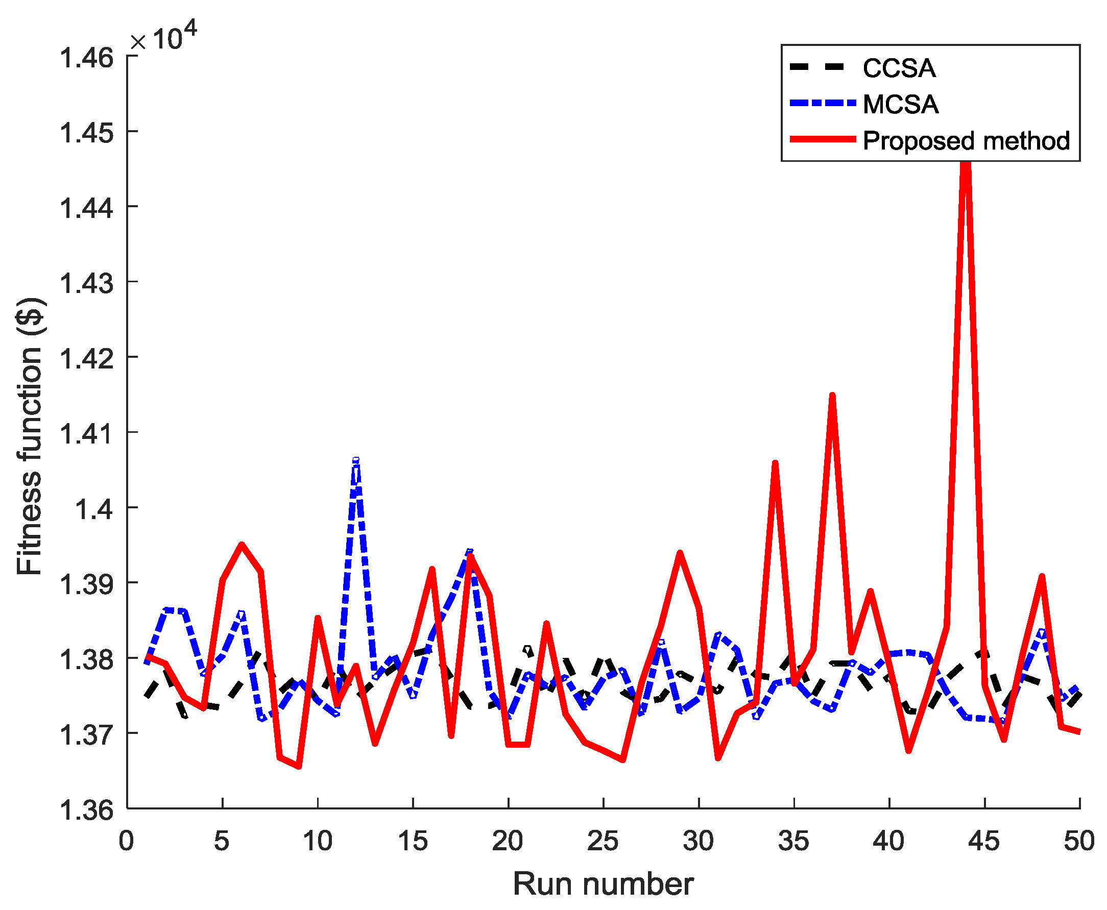
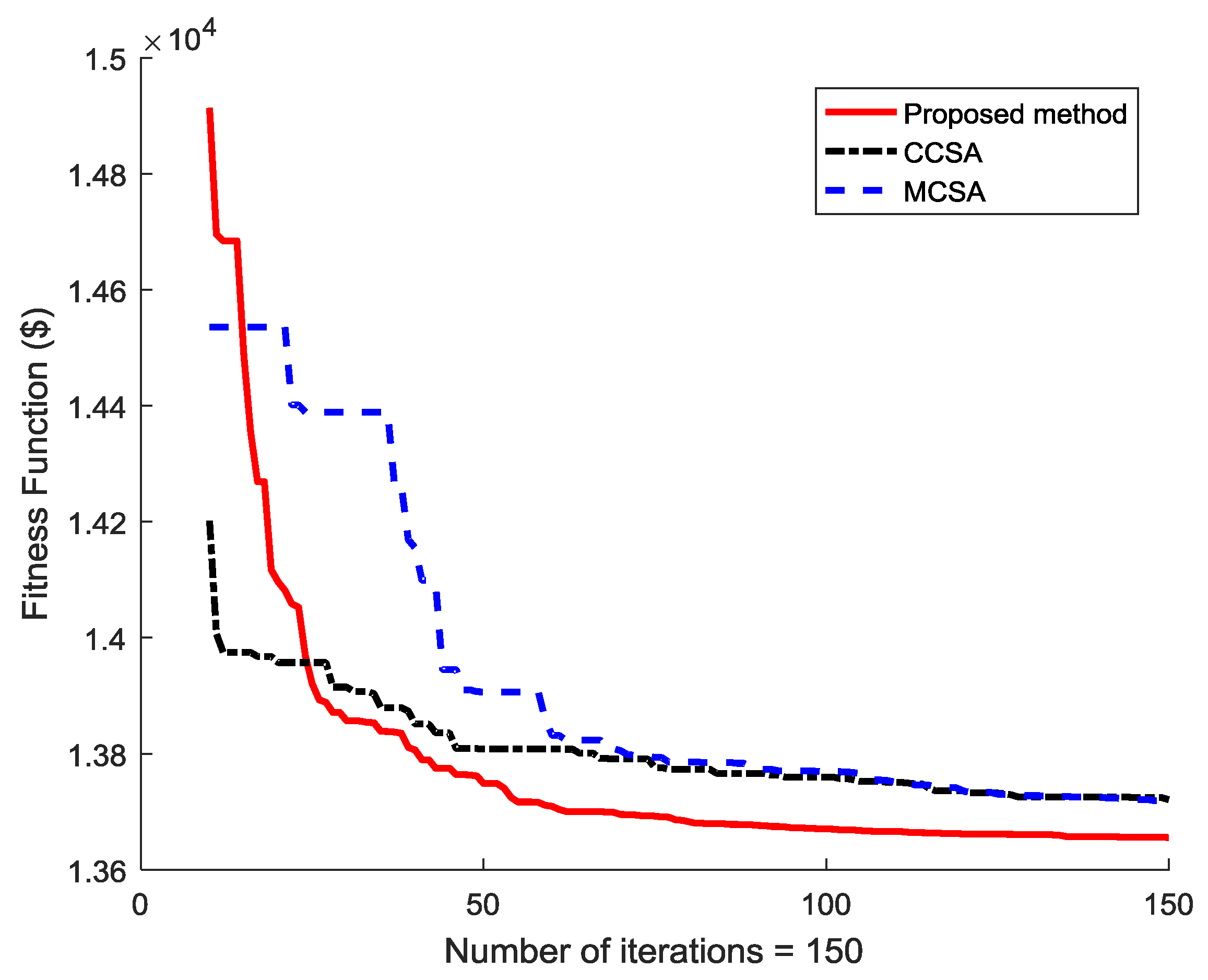
5.2. Results Obtained from the IEEE 30 Buses System

The test system comprises 30 buses, among which are six-generation buses, 24-load buses, and 41 branches. The information on the 30 IEEE buses systems, thermal units and hydro units is taken from [54]. The optimal operation plan is carried out in 24 h, divided into two 12-h optimal subintervals. The load of the first subinterval is fixed at values of the IEEE 30 buses system but the load of the second is reduced to 85% of the first subinterval. The data on the hydro and thermal units are listed

Table A1. Coefficients of cost function of four thermal units of the IEEE 30 buses system.

Unit No.	ai ($/h)	bi ($/MWh)	ci ($/MW2h)
1	0	2.00	0.00375
2	0	1.75	0.01750
3	0	1.00	0.06250
4	0	3.25	0.00834

and

Table A2. Hydraulic data of hydro units of the IEEE 30 buses system.

Hydro Plant	ahj (MCF/h)	bhj (MCF/MWh)	chj (MCF /MW2h)	Wj (MCF)
1	1.980	0.306	0.000216	200
2	0.936	0.612	0.000360	400

, respectively.

The results obtained from three applied methods such as minimum, average, maximum, standard deviation, and execution time, in addition to the SR for obtaining 50 successful runs, are shown in

Table 4. Comparison of obtained results for the IEEE 30 buses system.

Parameter	Method
	CCSA	MCSA	ENCSA
Pro	0.9	0.8	0.9
Min. cost ($)	13,722.208	13,718.230	13,655.538
Mean cost ($)	13,759.815	13,783.937	13,808.732
Max. cost ($)	13,815.143	14,066.094	14,548.909
Std dev. ($)	16.895	53.707	171.314
CPU time (s)	67.036	65.695	65.871
Successes rate (SR)	76%	91%	98%

. As observed from this table, that ENCSA has the lowest cost of $13,655.538 while MCSA has the second best ($13,718.230) and CCSA has the highest cost ($13,722.208). The exact comparison indicates that ENCSA has a lower cost than CCSA and MCSA by $66.67 and $62.692, respectively. Furthermore, ENCSA is also superior in its handling constraints over CCSA and MCSA because its SR is approximately 100%, whereas that of CCSA and MCSA is 76% and 91%, respectively. The SR of ENCSA is higher than that of CCSA and MCSA by approximately 22% and 7%, respectively, due to the contribution of the proposed selection technique-based dominant solutions. This result proves the benefit of the proposed selection technique-based dominant solutions in ENCSA, keeping the best candidates among N_p old solutions and N_p new solutions, as explained in Section 3.2. Moreover, the optimal value (lowest fuel cost) of ENCSA is the best solution among the compared methods. According to the general compared indices, we can conclude that ENCSA is more efficient than CCSA and MCSA when applied to solve the IEEE 30 buses system because it is superior among the three methods in having the lowest cost (optimal solution quality) and the highest SR (ability to deal with constraints).

Figure 3 depicts the convergence characteristics of fitness functions of the three methods. As observed in this figure, at the iteration of 25 there is a distinction in the performance of the ENCSA over CCSA and MCSA. In fact, at beginning iterations ENCSA obtains higher fitness function values than both CCSA and MCSA, but later it decreases dramatically and from the iteration of 25 to the final iteration the fitness function of ENCSA is much less than that of CCSA and MCSA. Furthermore, the improvement of the fitness functions in CCSA and MCSA is slight from the 50th iteration onward. Thus, we can conclude that applying the self-adaptive technique in ENCSA enhances the research ability and avoids convergence to a local optimum, while CCSA and MCSA can be easily trapped into the local optimal.

Summarily, ENCSA is superior to CCSA and MCSA in terms of fast convergence to a global optimum and higher SR thanks to the contribution of the proposed self-adaptive technique as well as the selection technique-based dominant solutions.

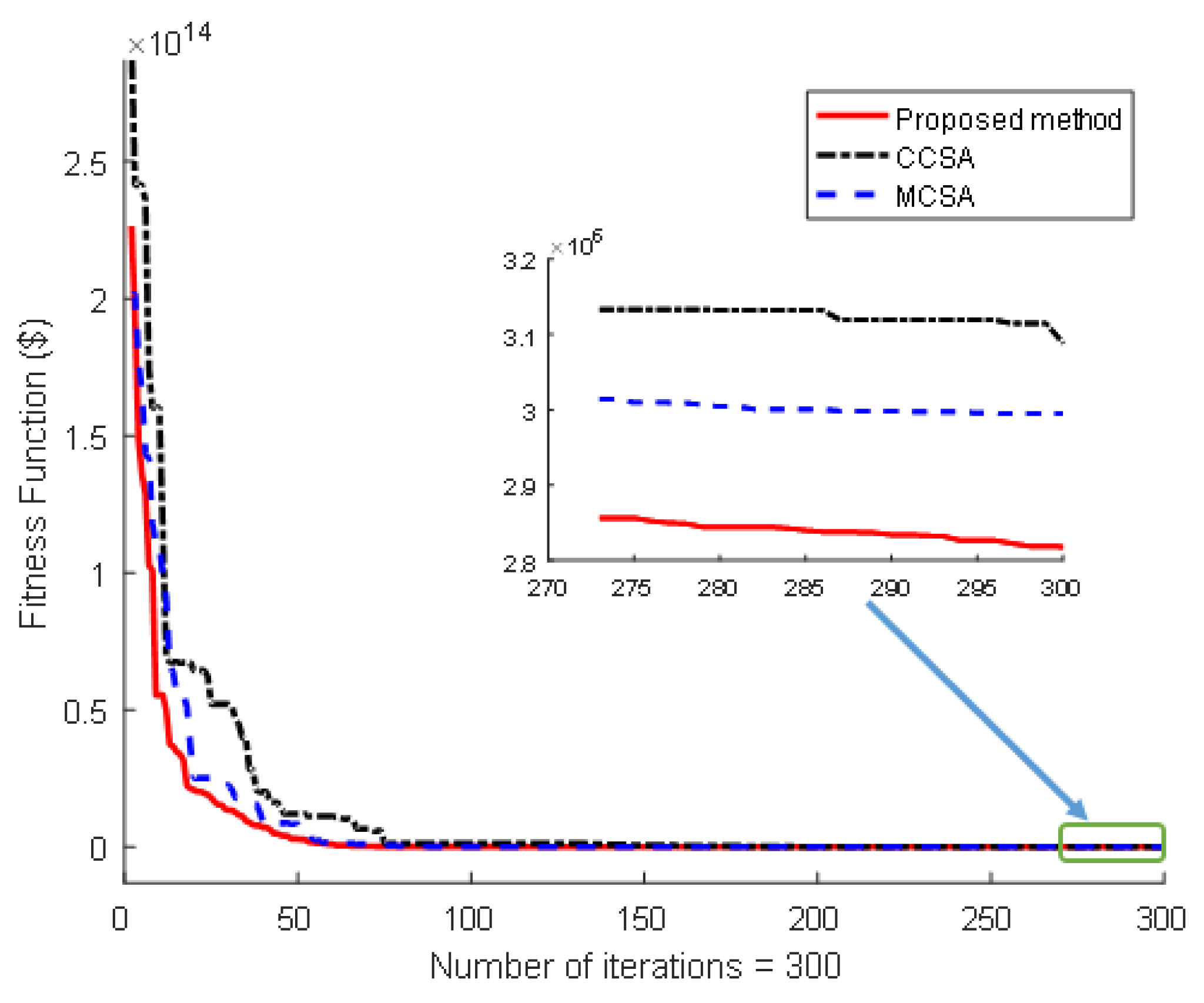
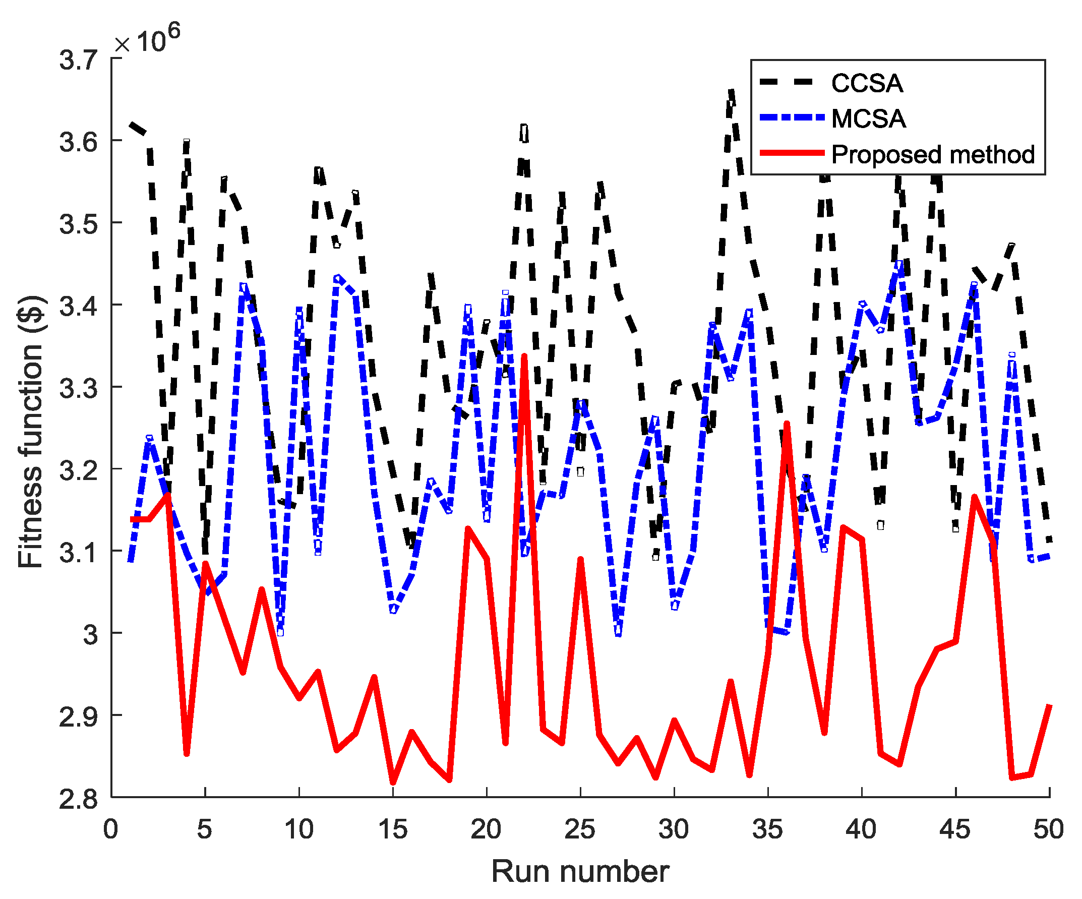
5.3. Obtained Results of the IEEE 118 Buses System

In this section, the IEEE 118 buses system [48], considering hydraulic constraints from reservoirs, generation capacity constraints of generators, and constraints from transmission lines, is employed to demonstrate the applicability of the CSA methods for dealing with a very large-scale system. The schedule time horizon is 24 h, divided into two subintervals including a 20 h subinterval and a 4 h subinterval. The load demand in the first subinterval is from the base case of the system and the load demand in the second is equal to 70% that of the first subinterval. The whole data of the IEEE 118 buses system is taken from [48] and other information on hydro and thermal units is taken from [54]. The data on the hydro units are given in

Table A3. The data of hydro units included in the IEEE 118 buses system.

Hydro Plant	Bus	ahj (MCF/h)	bhj (MCF/MWh)	chj (MCF/(MW)2h)	Wj (MCF)
1	111	1.0836	0.2159	0.000232	400
2	112	0.36	0.07197	7.73 × 10−5	120
3	113	1.0836	0.2159	0.000232	400
4	116	0.36	0.07197	7.73 × 10−5	120

.

The results comparison listed in

Table 5. Comparison of obtained results for the IEEE 118 buses system.

Parameter	Method
	CCSA	MCSA	ENCSA
Pro	0.9	0.9	0.8
Min. cost ($)	3,088,459.0	2,994,592.1	2,818,001.7
Mean cost ($)	3,358,689.2	3,216,312.3	2,961,433.3
Max. cost ($)	3,665,459.0	3,491,042.1	3,336,941.4
Std dev. ($)	153,667.7	129,941.3	123,993.9
CPU time (s)	278	286	282
SR	21%	46%	66%

reveals that ENCSA obtained the best minimum cost, the best standard deviation, and the highest SR ($2,818,001.70, $123,993.90, and 66%), while CCSA yields the worst results ($3,088,459.00, $153,667.70, and 21%). The best cost and standard deviation from ENCSA are less than those from CCSA by $270,457.30 and $29,673.80, respectively, and less than those from MCSA by $176,590.40 and $5947.40, respectively. In addition, the SR from ENCSA is also the best value among the three methods, at 66%. As observed in Figure 4, the performance of ENCSA over CCSA and MCSA is outstanding, where the searching speed (change rate of fitness values) of ENCSA is much greater than that of CCSA and MCSA for the first 60 iterations. After the 60th iteration later, the improvement still occurs in ENCSA but there is no significant improvement in CCSA and MCSA. Clearly, the impact of the self-adaptive technique on the performance can lead to a fast convergence to the global optimum and a high-quality solution; in addition, the impact of selection technique-based dominant solutions on the performance can lead to higher SR in ENCSA. Thus, we can conclude that ENCSA is the strongest method among the three compared methods due to the lowest minimum cost, the lowest standard deviation, and the highest SR. The optimal solutions obtained by ENCSA for the two test systems are shown in Table 4, Table 5 and

Table 6. The p values of Welch’s t-test for pairwise comparisons.

Tested System	Method	Size	Mean	Std.	t	df	p Value
30 buses	ASCSA	50	13,808.73	171.314	NA	NA	NA
	CCSA	50	13,759.82	16.895	2.0093251	0.08428355	≈0.3
	MCSA	50	13,783.94	53.707	2.30637854	0.01628009	≈0.3
118 buses	ASCSA	50	2,961,433.30	123,993.9	NA	NA	NA
	CCSA	50	3,358,689.20	153,667.7	14.2261863	1.2031E-07	<0.05
	MCSA	50	3,216,312.30	129,941.3	9.50689037	1.6885E-07	<0.05

.

5.4. Discussion of ENCSA and Further Analysis of Results

The proposed method has been developed with the aim of overcoming the disadvantages of CCSA such as the convergence to local optimums or near global optimums and a low SR for complicated systems. In the first improvement of ENCSA, we open the search zone as the current solution and the so-far best solution are close together and avoid adopting large jumping step missing promising zone with high-quality as current solution is far away the so-far best solution. Consequently, the first advantage of the proposed method over CCSA is to choose a suitable search zone for each considered solution. In the second improvement of ENCSA, all old and new solutions are mixed together and identical solutions are abandoned, keeping only one. Finally, the best N_p solutions are retained. Thus, the second advantage of ENCSA over CCSA is to retain N_p different solutions with higher quality than N_p abandoned ones. As to combining the two improvements, firstly, ENCSA can converge to a global optimum with faster speed than CCSA and secondly, ENCSA also gets a higher SR with optimal solutions, satisfying all constraints. However, ENCSA can also cope with several disadvantages that CCSA has not overcome, such as a high number of control parameters and the major effect of parameters on the obtained results. In fact, CCSA has three main parameters consisting of two basic ones of meta-heuristic algorithms—the population size (the number of nests) and the maximum number of iterations—and one advanced control parameter, the new solution update probability in each nest P_ro. The selection of the two basic control parameters is based on experience and the trial-error method, with a note that large-scale systems need a higher number of nests and a higher number of iterations. The selection of P_ro is not based on experience but should be set to a range from 0.1 to 0.9, and then the best P_ro is determined by evaluating the minimum fitness function and standard deviation. On the other hand, ENCSA has one more control parameter than CCSA, which is tol. The selection of tol is not dependent on the scale as well as the complex level of systems but should be set to a range consisting of five values such as 10⁻¹, 10⁻², 10⁻³, 10⁻⁴, and 10⁻⁵. Consequently, the selection of control parameters of ENCSA should be carefully tuned.

Further analysis of results: Derrac et al. [57] have pointed out that statistical tests should be performed for the obtained results in order to improve performance evaluation of different meta-heuristic algorithms, and the authors have presented the application of testing the sign and Wilcoxon rank-sum for the pairwise comparisons among results obtained by different methods. In Section 5.2 and Section 5.3, this paper has compared the results obtained by the proposed method with CCSA and MCSA with respect to the minimum cost, average cost, maximum cost, standard deviation, and SR. The results have indicated that the proposed method obtained a better minimum cost and higher SR than CCSA and MCSA for IEEE 30 and 118 buses power systems but other measures as the average cost, maximum cost, and standard deviation of the proposed method are lower than those of CCSA and MCSA (only for the IEEE 118 buses power system). For further investigation of the proposed method performance, we have chosen the Wilcoxon rank-sum test and Welch’s t-test for the analysis of results of the proposed method, CCSA, and MCSA. For implementation of the two tests on the two considered power systems, a level of significance α = 0.05 has been considered and obtained p values can result in two different cases, in which the first case is that p values are less than 0.05 and the second case is that p values are equal to or higher than 0.05. In the first case, the proposed method is a significant improvement; otherwise, the proposed method cannot provide solutions with a significant improvement over CCSA and MCSA [57]. The p values of Welch’s t-test and Wilcoxon’s rank-sum test are reported in Table 6 and

Table 7. The p values of Wilcoxon’s rank-sum test for pairwise comparisons.

Tested System	Method	p Value
30 buses	CCSA	0.184
	MCSA	0.251
118 buses	CCSA	0.0298
	MCSA	0.0312

, respectively. As shown in Table 6, the p values for comparison of the proposed method with CCSA and MCSA are approximately 0.3 for IEEE 30 buses hydrothermal power system and less than 0.05 for IEEE 118 buses hydrothermal power system. As observed in Table 7, p values are equal to 0.184 and 0.251, respectively, for an IEEE 30 buses hydrothermal power system corresponding to the comparison of the proposed method with CCSA and MCSA, and are 0.0298 and 0.0312, respectively, for IEEE 118 buses hydrothermal power system corresponding to the comparison of the proposed method with CCSA and MCSA. Clearly Welch’s t-test provides a range of p values, while Wilcoxon’s rank-sum test provides a particular value for each comparison. In spite of the difference, such numbers present the same results for evaluation. Both 0.184 and 0.251 are approximately equal to 0.3 and much higher than 0.05, while 0.0298 and 0.0312 are less than 0.05. Consequently, both Welch’s t-test and Wilcoxon’s rank-sum test point out that the proposed method is a significant improvement than CCSA and MCSA for IEEE 118 buses hydrothermal power system; however, the same evaluation is not seen for the IEEE 30 buses hydrothermal power system. The proposed method reached a success rate of 98%, while CCSA and MCSA have obtained success rates of 76% and 91%, respectively; thus, for 50 successful runs, the proposed method has executed only 51 runs while CCSA and MCSA have executed 66 and 55 runs, respectively.

The fitness function values obtained by the proposed method, CCSA, and MCSA over 50 successful runs are illustrated in Figure 5 and Figure 6 for the IEEE-30 bus system and the IEEE 118 buses system for further analysis on results. Figure 5 shows a high fluctuation of optimal solutions obtained by the proposed method, while CCSA and MCSA have smaller fluctuations. However, many red points of the proposed method have a lower fitness function than the black points of CCSA and blue points of MCSA, and such red points have approximate fitness values close to the best fitness. Clearly, the obtained results, the p-values of Welch’s t-test, and the p-values of Wilcoxon’s rank-sum test indicate the highly unstable search ability of the proposed method for the IEEE-30 bus system. In spite of this, the proposed method is still considered more effective than CCSA and MCSA because it finds a better optimal solution and many such better solutions nearby, while CCSA and MCSA cannot reach the zone near the optimal solutions of the proposed method. On the contrary, Figure 6 shows a completely different result since most red points of the proposed method have a much lower fitness function than the black points and blue points from CCSA and MCSA; even the best black point and the best blue point have a better fitness function than a few red points. In addition, the proposed method has a smaller fluctuation than CCSA and MCSA. Clearly, the obtained results, the p-values of Welch’s t-test, and the p-values of Wilcoxon’s rank-sum test can result in the same conclusion that the proposed method outperform CCSA and MCSA in terms of the best optimal solution and the stabilization of the search ability for the IEEE 118 buses system.

6. Conclusions

In this paper, an effective novel cuckoo search algorithm (ENCSA) has been proposed to deal with the optimal power flow problems of hydrothermal power systems, considering the constraints in transmission networks. The proposed method is an improved version of the conventional CSA in that it applies two techniques—the self-adaptive technique, which is used for the second step of generating new solutions, and the top solutions-based selection technique to keep the best solutions among all new and old solutions. To verify the performance of ENCSA, two tests cases have been implemented in the IEEE 30 and 118 buses systems. The results from both test cases have proved that ENCSA is a better method compared to CCSA and MCSA in terms of the optimal solution quality, success rate, and convergence speed. The self-adaptive technique can enable ENCSA to overcome the local optimum trap and the selection technique-based dominant solutions can allow ENCSA to reach a better optimal value faster. The results indicate that the proposed ENCSA is efficient at solving the hydrothermal optimal power flow problem.

References

1. El-Hawary, M.E.; Landrigan, J.K. Optimum operation of fixed-head hydro-thermal electric power systems: Powell’s Hybrid Method Versus Newton-Raphson Method. IEEE Trans. Power Appar. Syst. 1982, PAS-101, 547–554. [Google Scholar]
2. Wood, A.; Wollenberg, B. Power Generation, Operation and Control; Wiley: New York, NY, USA, 1996. [Google Scholar]
3. Zaghlool, M.F.; Trutt, F.C. Efficient methods for optimal scheduling of fixed head hydrothermal power systems. IEEE Trans. Power Syst. 1988, 3, 24–30. [Google Scholar] [CrossRef]
4. Rashid, A.H.A.; Nor, K.M. An efficient method for optimal scheduling of fixed head hydro and thermal plants. IEEE Trans Power Syst. 1991, 6, 632–636. [Google Scholar] [CrossRef]
5. Salam, M.S.; Nor, K.M.; Hamdam, A.R. Hydrothermal scheduling based Lagrangian relaxation approach to hydrothermal coordination. IEEE Trans. Power Syst. 1998, 13, 226–235. [Google Scholar] [CrossRef]
6. Basu, M. Hopfield neural networks for optimal scheduling of fixed head hydrothermal power systems. Electr. Power Syst. 2003, 64, 11–15. [Google Scholar] [CrossRef]
7. Sharma, A.K. Short Term Hydrothermal Scheduling Using Evolutionary Programming. Master’s Thesis, Thapar University, Patiala, India, 2009. [Google Scholar]
8. Basu, M. Artificial immune system for fixed head hydrothermal power system. Energy 2011, 36, 606–612. [Google Scholar] [CrossRef]
9. Farhat, I.A.; El-Hawary, M.E. Fixed-head hydro-thermal scheduling using a modified bacterial foraging algorithm. In Proceedings of the 2010 IEEE Electric Power and Energy Conference (EPEC), Halifax, NS, Canada, 25–27 August 2010; pp. 1–6. [Google Scholar] [CrossRef]
10. Sasikala, J.; Ramaswamy, M. Optimal gamma based fixed head hydrothermal scheduling using genetic algorithm. Expert Syst. Appl. 2010, 37, 3352–3357. [Google Scholar]
11. Kumar, B.R.; Murali, M.; Kumari, M.S.; Sydulu, M. Short-range Fixed head Hydrothermal Scheduling using Fast Genetic Algorithm. In Proceedings of the 2012 7th IEEE Conference on Industrial Electronics and Applications (ICIEA), Singapore, 18–20 July 2012; pp. 1313–1318. [Google Scholar]
12. Naranga, N.; Dhillonb, J.S.; Kothari, D.P. Scheduling short-term hydrothermal generation using predator prey optimization technique. Appl. Soft Comput. 2014, 21, 298–308. [Google Scholar] [CrossRef]
13. Dommel, H.W.; Tinny, W.F. Optimal power flow solution. IEEE Trans. Power Appar. Syst. 1968, PAS-87, 1866–1876. [Google Scholar] [CrossRef]
14. Stott, B.; Alsac, O.; Monticelli, A.J. Security analysis and optimization. Proc. IEEE 1987, 75, 1623–1644. [Google Scholar] [CrossRef]
15. Momoh, J.A.; Koessler, R.J.; Bond, M.S.; Stott, B.; Sun, D.; Papalexopoulos, A.; Ristanovic, P. Challenges to optimal power flow. IEEE Trans. Power Syst. 1997, 12, 444–447. [Google Scholar] [CrossRef]
16. Cain, M.B.; O’Neill, R.P.; Castillo, A. History of Optimal Power Flow and Formulations; FERC Staff Technical Paper; Federal Energy Regulatory Commission: Washington, DC, USA, 2012.
17. Thukaram, D.; Parhasarathy, K.; Khincha, H.P.; Narendranath, U.; Bansilal, A. Voltage stability improvement: Case studies if Indian power networks. Electr. Power Syst. Res. 1998, 44, 35–44. [Google Scholar] [CrossRef]
18. Yesuratnam, G.; Thukaram, D. Congestion management in open access based on relative electrical distances using Voltage stability criteria. Electr. Power Syst. Res. 2006, 77, 1608–1618. [Google Scholar] [CrossRef]
19. Nagendra, P.; Dey, S.H.n.; Datta, T.; Paul, S. Voltage stability assessment of a power system incorporating FACTS controllers using unique network equivalent. Ain Shams Eng. J. 2014, 5, 103–111. [Google Scholar]
20. Chen, G.; Lu, Z.; Zhang, Z. Improved Krill Herd Algorithm with Novel Constraint Handling Method for Solving Optimal Power Flow Problems. Energies 2018, 11, 76. [Google Scholar] [CrossRef]
21. Martinez, J.L.; Ramous, A.; Exposito, G.; Quintana, V. Transmission loss reduction by Interior point methods: Implementation issues and practical experience. Proc. IEE Gener. Transm. Distrib. 2005, 152, 90–98. [Google Scholar] [CrossRef]
22. Torres, G.L.; Quintana, V.H. An interior point method for non-linear optimal power flow using Voltage rectangular coordinates. IEEE Trans. Power Syst. 1998, 13, 1211–1218. [Google Scholar] [CrossRef]
23. Torres, G.L.; Quintana, V.H. Optimal power flow by a non-linear complementarity method. IEEE Trans. Power Syst. 2000, 15, 1028–1033. [Google Scholar] [CrossRef]
24. Oliveira, E.J.; Oliveira, L.W.; Pereira, J.L.R.; Honório, L.M.; Junior, I.C.S.; Marcato, A.L.M. An optimal power flow based on safety barrier interior point method. Electr. Power Energy Syst. 2015, 64, 977–985. [Google Scholar] [CrossRef]
25. Deb, K. Multi-Objective Optimization Using Evolutionary Algorithms; John Wiley and Sons, Inc.: New York, NY, USA, 2001. [Google Scholar]
26. Osman, M.S.; Abo-Sinna, M.A.; Mousa, A.A. A solution to the optimal power flow using genetic algorithm. Appl. Math. Comput. 2004, 155, 391–405. [Google Scholar] [CrossRef]
27. Yuryevich, J. evolutionary programming based optimal power flow algorithm. IEEE Trans. Power Syst. 1999, 14, 1245–1250. [Google Scholar] [CrossRef]
28. Abido, M.A. Optimal power flow using particle swarm optimization. Int. J. Electr. Power Energy Syst. 2002, 24, 563–571. [Google Scholar] [CrossRef]
29. El Ela, A.A.A.; Abido, M.A.; Spea, S.R. Optimal power flow using differential evolution algorithm. Electr. Power Syst. Res. 2010, 80, 878–885. [Google Scholar] [CrossRef]
30. Abido, M.A. Optimal power flow using tabu search algorithm. Electr. Power Compon. Syst. 2002, 30, 469–483. [Google Scholar] [CrossRef]
31. Bhattacharya, A.; Chattopadhyay, P.K. Application of biogeography-based optimisation to solve different optimal power flow problems. IET Gener. Transm. Distrib. 2011, 5, 70–80. [Google Scholar] [CrossRef]
32. Roa-Sepulveda, C.A.; Pavez-Lazo, B.J. A solution to the optimal power flow using simulated annealing. Int. J. Electr. Power Energy Syst. 2003, 25, 47–57. [Google Scholar] [CrossRef]
33. Vaisakh, K.; Srinivas, L.R.; Meah, K. Genetic eVolving ant direction particle swarm optimization algorithm for optimal power flow with non-smooth cost functions and statistical analysis. Appl. Soft Comput. 2013, 13, 4579–4593. [Google Scholar] [CrossRef]
34. Niknam, T.; Narimani, M.R.; Abarghooee, R.A. A new hybrid algorithm for optimal power flow considering prohibited zones and valve point effect. Energy Convers. Manag. 2012, 58, 197–206. [Google Scholar] [CrossRef]
35. Li, Y.Z.; Li, M.S.; Wu, Q.H. Energy saving dispatch with complex constraints: Prohibited zones, valve point effect and carbon tax. Electr. Power Energy Syst. 2014, 63, 657–666. [Google Scholar] [CrossRef]
36. Bouchekaraa, H.R.E.H.; Abido, M.A.; Boucherma, M. Optimal power flow using teaching-learning-based optimization technique. Electr. Power Syst. Res. 2014, 114, 49–59. [Google Scholar] [CrossRef]
37. Ghasemi, M.; Ghavidel, S.; Gitizadeh, M.; Akbari, E. An improved teaching–learning-based optimization algorithm using Lévy mutation strategy for nonsmooth optimal power flow. Electr. Power Energy Syst. 2015, 65, 375–384. [Google Scholar] [CrossRef]
38. Sayah, S.; Zehar, K. Modified differential evolution algorithm for optimal power flow with non-smooth cost functions. Energy Convers. Manag. 2008, 49, 3036–3042. [Google Scholar] [CrossRef]
39. Amjady, N.; Sharifzadeh, H. Security constrained optimal power flow considering detailed generator model by a new robust differential evolution algorithm. Electr. Power Syst. Res. 2011, 81, 740–749. [Google Scholar] [CrossRef]
40. Tan, Y.; Li, C.; Cao, Y.; Lee, K.Y.; Li, L.; Tang, S.; Zhou, L. Improved group search optimization method for optimal power flow problem considering valve-point loading effects. Neurocomputing 2015, 148, 229–239. [Google Scholar] [CrossRef]
41. Bakirtzis, A.G.; Biskas, P.N.; Zoumas, C.E.; Petridis, V. Optimal power flow by enhanced genetic algorithm. IEEE Trans. Power Syst. 2002, 17, 229–236. [Google Scholar] [CrossRef]
42. Reddy, S.S.; Bijwe, P.R.; Abhyankar, A.R. Faster evolutionary algorithm based optimal power flow using incremental variables. Electr. Power Energy Syst. 2014, 54, 198–210. [Google Scholar] [CrossRef]
43. Alsac, O.; Scott, B. Optimal power flow with steady state security. IEEE Trans. Power Appar. Syst. 1974, 93, 745–751. [Google Scholar] [CrossRef]
44. Lai, L.L.; Ma, J.T.; Yokoyama, R.; Zhao, M. Improved genetic algorithms for optimal power flow under both normal and contingent operation states. Electr. Power Energy Syst. 1997, 19, 287–292. [Google Scholar] [CrossRef]
45. Sivasubramani, S.; Swarup, K.S. Multi-agent based differential evolution approach to optimal power flow. Appl. Soft Comput. 2012, 12, 735–740. [Google Scholar] [CrossRef]
46. Soliman, A.; Mantawy, A.H. Modern Optimizati on Techniques with Applications in Electric Power Systems; Springer: New York, NY, USA, 2010. [Google Scholar]
47. Elsaiah, S.; Cai, N.; Benidris, M.; Mitra, J. A Fast Economic Power Dispatch Method for Power System Planning Studies. IET Gener. Transm. Distrib. 2015, 9, 417–426. [Google Scholar] [CrossRef]
48. El-Hawary, M.E.; Tsang, D.H. The Hydrothermal Optimal Load Flow, A Practical Formulation and Solution Techniques Using Newton’s Approach. IEEE Trans. Power Syst. 1986, 1, 157–166. [Google Scholar] [CrossRef]
49. Habibollahzadeh, H.; Semlyen, G.X.L.A. Hydrothermal optimal power flow based on a combined linear and nonlinear programming methodology. IEEE Trans. Power Syst. 1989, 4, 530–537. [Google Scholar] [CrossRef]
50. Angelidis, G. Short-term Optimal Hydrothermal Scheduling Problem Considering Power Flow Constraint. Can. J. Elect. Comp. Eng. 1994, 19, 81–86. [Google Scholar] [CrossRef]
51. Wei, H.; Sasaki, H.; Kubokawa, J. Interior point method for hydro-thermaloptimal power flow. In Proceedings of the 1995 International Conference on Energy Management and Power Delivery (EMPD ‘95), Singapore, 21–23 November 1995; Volume 2, pp. 607–612. [Google Scholar]
52. Wei, H.; Sasaki, H.; Kubokawa, J.; Yokoyama, R. Large Scale Hydrothermal Optimal Power Flow Problems Based on Interior Point Nonlinear Programming. IEEE Trans. Power Syst. 2002, 15, 396–403. [Google Scholar] [CrossRef]
53. Lin, S.; Huang, J.; Zhang, J.; Tang, Q.; Qiu, W. Short-term optimal hydrothermal scheduling with power flow constraint. In Proceedings of the 27th Chinese Control and Decision Conference (2015 CCDC), Qingdao, China, 23–25 May 2015; pp. 1189–1194. [Google Scholar]
54. Nguyen, T.T.; Vo, D.N.; Truong, A.V.; Ho, L.D. Meta-Heuristic Algorithms for Solving Hydrothermal System Scheduling Problem Considering Constraints in Transmission Lines. Glob. J. Technol. Optim. 2016, 7, 1–6. [Google Scholar] [CrossRef]
55. Yang, X.S.; Deb, S. Cuckoo search via Lévy flights. In Proceedings of the World Congress on Nature & Biologically Inspired Computing (NaBIC 2009), Coimbatore, India, 9–11 December 2009; pp. 210–214. [Google Scholar]
56. Walton, S.; Hassan, O.; Morgan, K.; Brown, M.R. Modified cuckoo search: A new gradient free optimisation algorithm. Chaos Solut. Fractals 2011, 44, 710–718. [Google Scholar] [CrossRef]
57. Derrac, J.; Molina, G.S.D.; Herrera, F. A practical tutorial on the use of nonparametric statistical tests as a methodology for comparing evolutionary and swarm intelligence algorithms. Swarm Evolut. Comput. 2011, 1, 3–18. [Google Scholar] [CrossRef]
Figure 1. Two ways for updating the second new solution generation.
Energies 11 00188 g001
Figure 2. The flowchart of using the proposed method to solve the considered problem.
Energies 11 00188 g002
Figure 3. Fitness function convergence characteristics for the IEEE 30 buses system.
Energies 11 00188 g003
Figure 4. Fitness function convergence characteristics for the IEEE 118 buses system.
Energies 11 00188 g004
Figure 5. Fitness function values obtained by CCSA, MCSA, and the proposed method over 50 runs for the IEEE 30 buses system.
Energies 11 00188 g005
Figure 6. Fitness function values obtained by CCSA, MCSA, and the proposed method over 50 runs for the IEEE 118 buses system.
Energies 11 00188 g006