Stochastic Model Predictive Fault Tolerant Control Based on Conditional Value at Risk for Wind Energy Conversion System


Key Lab of Field Bus and Automation of Beijing, North China University of Technology, Beijing 100144, China
*
Author to whom correspondence should be addressed.
Energies 2018, 11(1), 193; https://doi.org/10.3390/en11010193
Submission received: 20 December 2017
/
Revised: 5 January 2018
/
Accepted: 10 January 2018
/
Published: 12 January 2018
(This article belongs to the Special Issue Emerging Power Electronics Technologies for Power Systems and Machine Drives)
Abstract
:Wind energy has been drawing considerable attention in recent years. However, due to the random nature of wind and high failure rate of wind energy conversion systems (WECSs), how to implement fault-tolerant WECS control is becoming a significant issue. This paper addresses the fault-tolerant control problem of a WECS with a probable actuator fault. A new stochastic model predictive control (SMPC) fault-tolerant controller with the Conditional Value at Risk (CVaR) objective function is proposed in this paper. First, the Markov jump linear model is used to describe the WECS dynamics, which are affected by many stochastic factors, like the wind. The Markov jump linear model can precisely model the random WECS properties. Second, the scenario-based SMPC is used as the controller to address the control problem of the WECS. With this controller, all the possible realizations of the disturbance in prediction horizon are enumerated by scenario trees so that an uncertain SMPC problem can be transformed into a deterministic model predictive control (MPC) problem. Finally, the CVaR object function is adopted to improve the fault-tolerant control performance of the SMPC controller. CVaR can provide a balance between the performance and random failure risks of the system. The Min-Max performance index is introduced to compare the fault-tolerant control performance with the proposed controller. The comparison results show that the proposed method has better fault-tolerant control performance.
1. Introduction
Wind energy is drawing considerable attention as an important kind of green energy [1]. Wind turbines with variable speed and pitch angle have become the main Wind Energy Conversion System (WECS) since they have the advantages of maximizing wind energy capture and providing stable output power. However, WECSs have many real difficulties such as high rates of facility faults, maintenance inconvenience caused by their poor reliability, and high outage losses [2,3]. Therefore, how to realize the fault-tolerant control of WECS is significant to improve the utilization rate of wind energy and reduce maintenance costs.
Modeling WECSs and investigating suitable controllers are hard since they are mathematically integrated with the characteristics of high order, multi-variable and strong coupling. Meanwhile, the randomness of wind speed magnitude and direction, the fluctuation of the grid parameters, and the atmospheric conditions are all possible disturbances of a WECS, which makes the WECS a typical stochastic hybrid system. Scenario-based stochastic model predictive control (SMPC) has been one of the hot topics in the field of model predictive control in recent years, which is a good control method for stochastic Markov jump liner systems. The advantage of Scenario-based SMPC is that it can consider the full probability information of the disturbance for prediction. The SMPC approach has been applied in constrained network control systems [4], energy management [5], and stock option market studies [6,7,8,9]. In [10], Bemporad proposed the Discrete Hybrid Stochastic Automata (DHSA) model and gave an SMPC optimization algorithm of this model. However, this algorithm only considers the expected optimal performance index of the system under normal conditions, without considering the random failure risk of the discrete hybrid system. To the authors’ limited knowledge, the scenario-based SMPC has not been applied to solve the control problem of WECS [11].
For the fault problems of WECSs, in recent years, there is a great deal of research work focusing on the fault-tolerant control of WECS [12,13,14,15,16,17,18,19]. Shahbazi [12] designed a six/five-leg converter to realize active fault-tolerant control for open-circuit switch faults to solve unknown but bounded noise and modeling errors. In [13], an adaptive step-by-step sliding mode observer and a compensation fault-tolerant control (FTC) strategy were developed for wind turbine pitch systems to maintain nominal pitching performance and compensate the considered low pressure actuator faults. Schulte [14] presented a T-S sliding mode observer for actuator fault diagnosis and fault compensation fault-tolerant control of hydrostatic transmission wind turbine. For a WECS system at a given operating point, Shi [15] formulated its Stochastic Piece Wise Affine (SPWA) model and implemented fault-tolerant control of WECS. The main limitation of the current research on WECS modeling and fault-tolerant control is that it does not provide a thorough description of the stochastic and nonlinear switching dynamic characteristics of wind turbines at random wind speeds. Some works regard the wind speed as a Gaussian or bounded disturbance [15,20], thus failing to fully discover the statistical properties of wind speed. To the authors’ limited knowledge, there is no fault-tolerant control research on WECS with actuator faults under real-time and random wind speed conditions in the literature.
Model Predictive Control (MPC) is an advanced fault-tolerant control method since it has many benefits arising from its features, such as prediction model [21,22,23], constraints [24,25,26], objective function [23,27], etc. Based on these features, the MPC controller can effectively deal with the influence on a WECS suffering from a fault. Notably, how to properly adjust the objective function of an MPC controller for fault-tolerant control is a very attractive research area [28]. Most of the existing research works on fault-tolerant model predictive control use the objective function adding the fault loss to realize a penalty on the objective function. However, this objective function cannot completely describe the fault risk of the WECS. CVaR is a performance indicator that can provide a balance between the performance and random failure risks of the system and it can achieve optimal performance control in the event the system runs into failure with a certain probability. CVaR is widely used for risk measurement in areas such as finance [29,30], energy [31], etc. The main advantages of CVaR are as follows [29]: (1) it is a coherent risk measure that satisfies variability, orthonormality, subadditivity and monotonicity; (2) it satisfies convexity, and can be transformed into a linear programming problem which is easy to solve.
This paper focuses on the fault-tolerant control of WECS, and proposes a new scenario-based SMPC fault-tolerant controller with the Conditional Value at Risk (CVaR) objective function. First, a linear stochastic Markov jump linear model is used to describe the nonlinear switching of wind turbines and stochastic factors in WECS, which fully uses the probability information of the wind. Second, the scenario-based SMPC controller is used as the controller to solve the control problem of WECS. With this controller, all the possible realizations of the disturbance in the prediction horizon are enumerated by scenario trees, so that the uncertain stochastic model predictive control problem can be transformed into a deterministic model predictive control problem. Besides, the online optimization property of SMPC can incorporate many important factors to enable the control of systems subject to faults and changing dynamics. Finally, to improve the fault-tolerant control performance, the CVaR objective function is adopted in the scenario-based SMPC controller. With CVaR objective function, a certain risk probability is transformed into a Linear Programming (LP) problem, and the fault-tolerant control performance of WECS probabilistic failures is guaranteed. The Min-Max index is introduced to compare with the proposed method [32]. The comparison results suggest that the proposed method has better fault-tolerant control performance than the controller with Min-Max index.
This paper is organized as follows: Section 2 formulates the Markov Jump Linear Model of WECS. Section 3 designs the scenario-based SMPC controller. In Section 4, the design of our SMPC fault-tolerant controller is presented. Section 5 is the simulation results and analysis. Conclusions are drawn in Section 6.
2. Markov Jump Linear Model of Wind Energy Conversion System
Wind turbines exhibit complex nonlinear characteristics and the stochastic wind speed causes the frequent switching of wind turbine operating points. The Markov jump system has been well investigated due to the probabilistic description of model parameters switching induced by external causes (e.g., random faults, unexpected events, uncontrolled configuration changes). In this section, a Markov jump linear model is established for the wind turbine to describe the switching of the system between different operating conditions (e.g., normal and faulty). For the specified wind turbine, it can sample the low-frequency wind speed data in separate speed intervals. With these sampled data, the stochastic characteristic of the wind speed can be represented as a Markov process, and then the traditional operating points of the wind turbine can be divided into separate sub regions, where the model parameters and the control mode can be fixed in each region. In this section, the Markov Transition Matrix of the Wind Speed is introduced first, and then the modeling process of the WECS is given.
2.1. Markov Transition Matrix of the Wind Speed
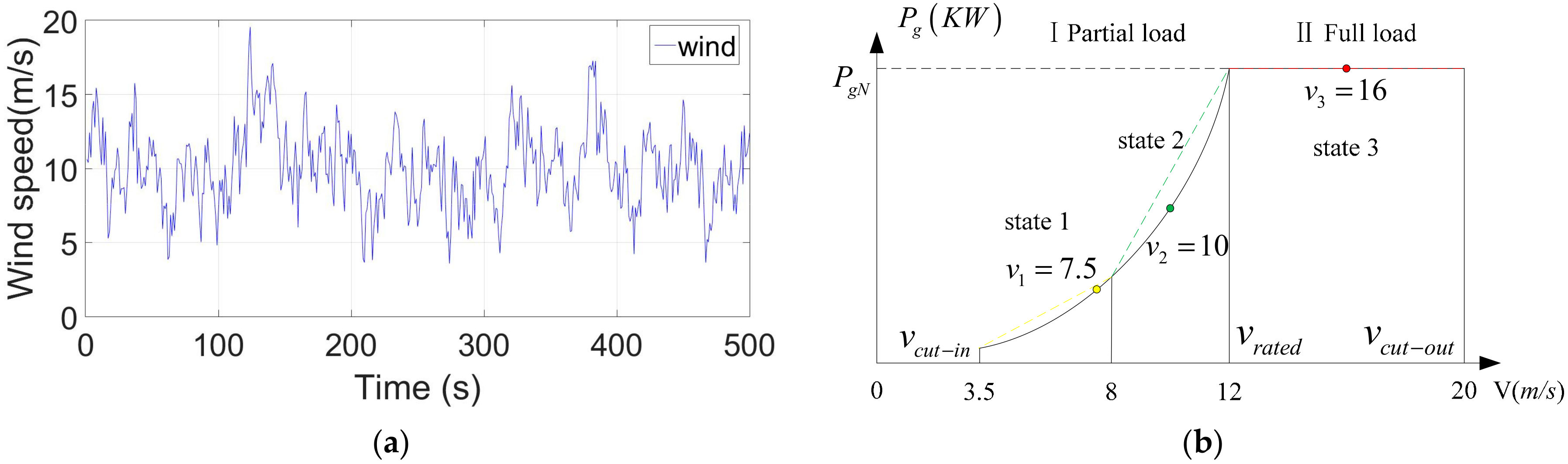
Given a set of continuous wind speed data, as shown in Figure 1a, the relationship between wind speed and generator power is given in Figure 1b. In Figure 1b, is the cut-in wind speed, is the rated wind speed, and is the cut-out wind speed. When , the WECS does not start, and its generated power . When , WECS should adjust its pitch angle to minimize the wind energy capture, brake the system, and disconnect it from the grid. When , the WECS is working in the partial load region, and the control objective is to maximize the harvested wind power. During , the wind speed is divided into three sections, corresponding to the three working states of WECS .
To illustrate the switching characteristics of the wind speed, we define the wind speed status intervals as follows:
and the working state points are , , .
To make the Markov Transition Matrix of the wind speed more accurate, it can take multiple wind speed intervals (i.e., , etc.). However, adding intervals will increase the computational burden, therefore, this paper only chooses three working state points to calculate the Markov Transition Matrix.
The one-step probability transition matrix P of the wind speed contains the probability information of the wind speed time series [33]. This paper uses statistical method to calculate the one-step Markov Transition Matrix. To take the advantages of Markov chain theory, the wind speed is discretized into , . The state transition probability of the wind speed is the probability that the state of wind speed is (i.e.,) in period t, and is in period t + 1, :
Let denote the number of wind speeds that were in state at time t and are in state at time , then:
The one-step transition matrix could be expressed as:
where [34].
2.2. Modeling of Wind Energy Conversion System
The inputs of the Wind Energy Conversion System (WECS) (Figure 2) are the wind speed , generator torque reference and pitch angle reference . The outputs of the system are generator speed and generator power .
2.2.1. Aerodynamics Model
The power captured by the rotor is:
where is the rotor swept area, is the rotor effective wind speed, is the air density, and is the power coefficient.
The tip-speed ratio is defined as the ratio between the tip speed of the blades and the rotor effective wind speed:
where is the rotor speed, and is the blade length.
2.2.2. Drive Train Model
The drive train dynamics function is given:
where and are the moments of inertia of the low-speed and high-speed shaft; is the gear ratio; is the torsion damping coefficient of the drive train; is the torsion stiffness of the drive train; is the twist of the flexible drive train with . and are the viscous friction of the high and low speed shaft, respectively. is the aerodynamic torque applied to the rotor.
2.2.3. Pitch System Model
The hydraulic pitch system can be modeled by a second order transfer function [37], described as:
where is the damping ratio of the pitch actuator model.
2.2.4. Generator and Converter Model
The generator and converter dynamics can be approximated by a first-order system:
where is the time constant.
The real-time power is described by:
2.2.5. The Dynamics of the Wind Energy Conversion System
Combining Equations (5)–(10), the dynamics of the WECS can be obtained:
Let be the state, be the input, be the disturbance. Then a linearized overall state space model describing the dynamics of the WECS can be given:
. and are the linearized parameters in different wind speed state working points (see Table 1).
In Equation (12), the wind speed can be considered as a combination of the mean wind speed and a stochastic component :
where is the average wind speed, corresponding to low-frequency variation; and is the fast, high-frequency variation.
Following [37,38,39], the stochastic component can be approximated by a linear second order transfer function driven by a white noise process:
where ,, and are parameters depending on the mean wind speed.
Finally, the dynamics of WECS can be obtained:
2.2.6. Discrete Markov Jump Linear Model of Wind Energy Conversion System
This paper adopts the tracking control algorithm with augmented state variables [41]. Discretize and linearize model (15) at three operating points where wind speed is 7.5, 10 and 16 m/s, respectively. Then it can get the WECS discrete-time linear system:
where , is the time index, is the output reference, is the state, is the input, is the disturbance, and R is a finite set. , , and are the system model matrixes corresponding to the three working states of WECS . Model (16) jumps stochastically from state to state with wind speed Markov transition probability introduced in Section 2.1.
3. Design of Scenario-Based Stochastic Model Predictive Controller
3.1. Scenario Tree Design
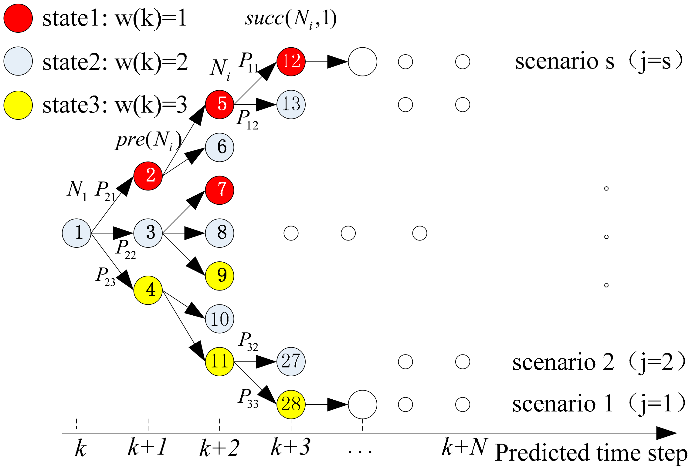
According to the Markov Transition Matrix described in the Section 2.1, we can build a scenario tree to describe the possible disturbance realization at every time step in the future. Let us make the following definition [42]:
- (1)
- : the set of the tree nodes. (i.e., is the root node and is the leaf node);
- (2)
- : the predecessor of node ;
- (3)
- : the successor of node ;
- (4)
- , , : the state, input and disturbance of node , respectively. Where , ;
- (5)
- : the set of leaf nodes.
The scenario tree is shown in Figure 3. In Figure 3, each node represents a system state in the prediction horizon. Red, yellow and gray represent three different states (), respectively. The abscissa axis represents the predicted horizon, which starts from time and end at time . The scenarios number is equal to the leaf nodes number at the termination moment .
The numbering method of the scenario node is numbered from the root node to the leaf node sequentially when they are added to the scenario tree. Each path of the scenarios represents a disturbance realization of the optimization problem. However, the number of nodes in the scenario tree generated in this way will increase exponentially with the prediction horizon. From an engineering point of view, it makes no sense to consider far-reaching disturbances in the prediction horizon, as the MPC controller runs in a receding horizon manner [43]. After a certain layer of the scenario tree, we assume that the disturbances are the same as the nodes corresponding to the layers , and extend to the prediction horizon . In this way, the complexity of the problem will be reduced to linear from the exponential order .
Here, it only shows the case root node , and are similar. At every time step online, the prediction is the scenario tree with the root node . Therefore, it can generate three scenario trees based on different root nodes, and calculate the corresponding controller . When implementing receding horizon optimization, call the controller according to the current state of the system.
In Figure 3, each scenario has its own evolution. For the sake of simplicity, it uses , , , and to denote , , , and , respectively. The state equation of a scenario transferred from the previous node to the current node is:
and the transition probability of (16) is:
where is calculated in Section 2.1.
3.2. Control Problem Formulation
In a general point of view, the optimization object of the stochastic model predictive control is the following equation:
where is expectation, is the state reference, is the input at prediction time step in the scenario tree (Figure 3).
To solve problem (19), this paper considers the realization and the probability of the disturbance to minimize the quadratic function performance index of state and input. In other words, the common quadratic performance index of scenario , multiplied by the probability of its realization, is the expectation of scenario . With this procedure, the expectation is transformed into a simple sum of all the , which makes an easy way to solve problem (19). In this way, the uncertain SMPC problem can be transformed into a deterministic MPC problem. At time k, based on the scenario trees, the following stochastic MPC problem is formulated:
where is the realization probability of scenario . and are the weight matrixes. is the current state of the system. and are coefficient matrixes in state and input constrains. Problem (20) is a quadratic constrained quadratic programming (QCQP) problem. The input of the root node is the first element of the solution to the problem (20). Problem (20) is an open-loop optimization problem, and the real-time control law is obtained by receding horizon optimization.
4. Design of Stochastic Model Predictive Fault Tolerant Controller
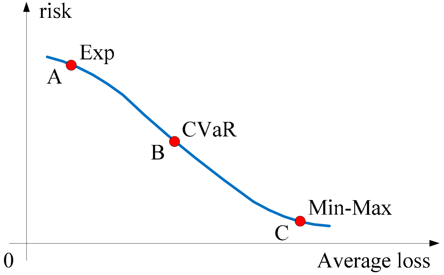
For a stochastic system with fault risk, system performance and system risk are two independent system events, and there are two kinds of classic control methods: (1) When increasing the proportion of system performance in the control target, the average system loss is reduced and the system risk is increased; (2) When increasing the proportion of system risk in the control target, the average system loss is increased and the system risk is decreased. The relationship of the system performance and system risk is represented in Figure 4. To achieve the first control method, the expectation performance index is introduced into the standard SMPC optimal control algorithm [10] as shown in Figure 4 (point A). Expectation optimization algorithm can get better system performance, but it will increase the risk of system failure. In some extreme cases, it may bring irreparable damage to the system. To achieve the second control method, the Min-Max optimization control algorithm is introduced to minimize the risk of the system [32], as shown in Figure 4 (point C). Although the Min-Max optimization algorithm ensures the system security and has better fault-tolerant performance, its control law is too conservative, which seriously reduces the system performance.
To address the issues of the two control methods mentioned above, the CVaR is introduced in this paper. The CVaR makes a balance between system performance and failure risk so that it can make a trade-off according to the specific control problem. By introducing CVaR to SMPC framework, this paper proposes a new fault-tolerant control optimization algorithm. Its relationship between the performance and the risk is shown in Figure 4 (point B).
4.1. Actuator Failure of Wind Energy Conversion System
This article only considers actuator failure, and the proposed method is also suitable for the sensor failure. Consider the discrete random model of a WECS with actuator gain loss:
where is the loss of gain under risk, is the partial loss of the actuator fault. The relationship between the gain loss under risk and the degree of system failure is shown in Table 2, where is a second order diagonal matrix.
4.2. Design of CVaR Fault Tolerant Controller
Conditional value at risk is a new stochastic calculation method to solve the optimization problem of WECS. This algorithm can figure out the optimal control law under different probability levels ,, and it can effectively deal with the impact of extreme conditions beyond the level . Conditional value at risk is defined as following.
Let be a loss function associated with the decision vector and random disturbances . is the probability density of . For a given probability , the (value at risk) is defined as the lowest risk value . is a fixed value, usually or . The main drawback of is that the information of extreme loss occurring with probability () is not considered directly. To avoid this, Rockafellar [29] introduced the concept of Conditional Value at Risk (CVaR). CVaR can quantify the average value that the loss function exceed , with probability . Therefore, it can calculate , and then solve the performance index.
4.2.1. Evaluate
There are many ways to calculate VaR, such as historical simulation, Monte Carlo simulation and variance-covariance method. Among them, the historical simulation method is a widely used approach [44,45].
The probability of which is not exceeding the threshold is:
where is the prediction error, is the output and is the output reference. Assuming its distribution is shown as Figure 5
In Figure 5, is defined as:
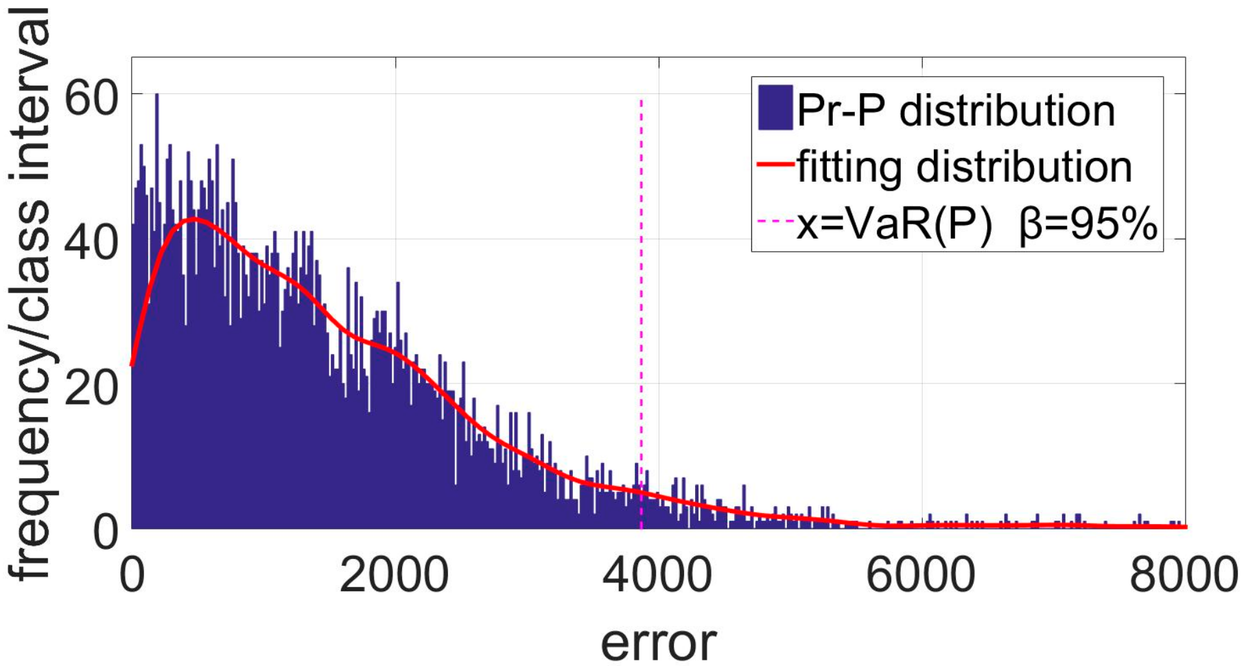
If the probability density of is calculated, then the value of () can be found. The probability density of can be statistically derived from the operational data of WECS, as shown in Figure 6.
The probability density curve of the output error is similar to Figure 6. While , by statistics, the value of are , .
4.2.2. Minimization of Conditional Value at Risk (LP-CVaR)
is defined as:
The loss function of is related to the decision vector , and it is could be determined by the formula:
where:
It is hard to get an explicit expression of (26). Therefore, CVaR is usually calculated through discretization. is sampled in its probability density . If there are trajectories of disturbance realization in SMPC, the probability of scenario is . Then the approximate value of (26) can be expressed as:
Let , the scenario-based SMPC problem can be redefined using the CVaR performance index [46]:
where is the prediction of path , represents excess loss over VaR. The fault-tolerant control of CVaR is to penalize the excess losses:
where , , , and contain the jumping information of prediction trajectory .
When is given, is a constant, and (28) can be rewritten as:
where:
Let , Equation (31) is transformed into a standard linear programming problem (LP) [47]. This description could have all the scenario information. The input of the root node is the first element of the solution to Problem (31). Problem (31) is an open-loop optimization problem, and the SMPC control law is obtained in a receding horizon manner. The Algorithm 1 is as follow:
| Algorithm 1: SMPC algorithm of CVaR objective function |
| 1. Prepare the controller |
| 1.1. Generate scenario trees according to different root node |
| 1.2. Calculate corresponding controllers |
| 2. Calculate VaR |
| set ; |
| solve SMPC problem (20); |
| The VaR is given by (22), (23); |
| 3. Calculate SMPC of CVaR |
| for i = 1:3 |
| % decision vectors weights |
| Calculate other parameters; |
| end for |
| set ; %Simulation time |
| for k = 1:T |
| measure (or estimate) ; |
| solve CVaR SMPC problem (31) and obtain ; |
| apply ; |
| end for |
4.3. Design of Min-Max Fault Tolerant Controller
In 1996, Kothare [32] proposed LMI-based robust predictive control for polytopic uncertain systems. When the model parameters change arbitrarily in the polytopic, this algorithm gives the optimal infinite horizon quadratic performance index under the worst case.
Considering the discrete-time linear system (16), let be the system state reference and be the input reference, the:
According to the method of dealing with the unnominal system in [48], the model (16) is processed as follows. According to the (16)–(39), it derives:
Then (40) becomes a regulation problem of a nominal system. According to the solution of Min-Max MPC optimization problem, we have:
where F is the state feedback control law.
From (39):
Substituting (42) into (41) yields:
Then the receding horizon control law is obtained by solving Equation (43) online.
5. Simulation Result and Analysis
To verify the effectiveness of scenario-based SMPC in WECS control under normal operating conditions and good fault tolerance performance of CVaR performance indicator, the WECS model (15) is discretized and linearized to model (16) at three operating points where wind speed is 7.5, 10 and 16 m/s, respectively. Then we use the algorithm mentioned above to track the constant value and dynamic set points generated by WECS under real-time wind.
The following WECS stochastic model of (16) can be obtained according to the modeling process in Section 2.2. The input and state constraints , , prediction horizon , scenario tree layer , the Markov transition matrix , weight matrix , .
Here, the method of LMI-based RMPC mentioned in [32] is used by the Min-Max performance index. For the model (16), the feedback control law is:
The simulation runs on an environment equipped with an Intel(R) Core(TM) i7-4770 CPU 3.40GHz RAM 8GB, using Matlab R2015a. The major computation burden is solving an instance of the QCQP (20) and of the LP (31), which costs 2.0 and 1.6 ms, respectively.
5.1. Wind Energy Conversion SystemTracking Constant Value when Normal
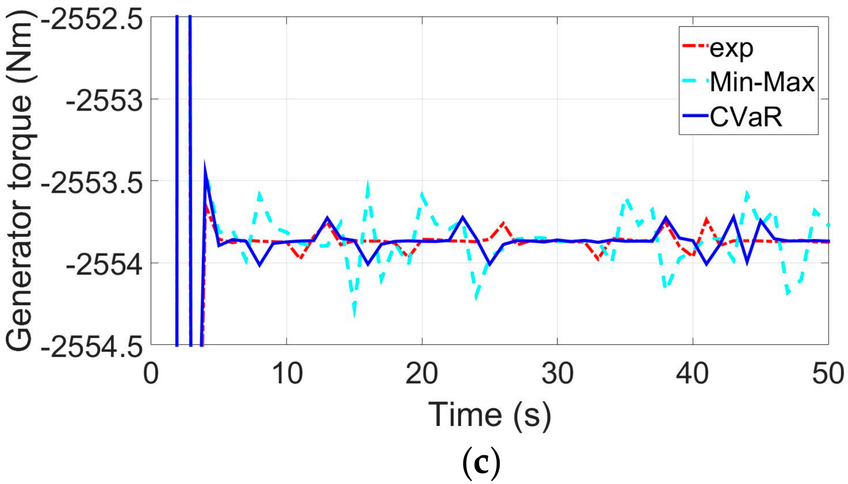
The simulation is adopted to verify the control performance of the SMPC controller with three different objective functions (Exp, CVaR, Min-Max). The control purpose is making the generator speed and generator power track constant values under random wind speed (the generator power ’s reference is 114,974 W. The fluctuations of are small, and we do not show them here). As shown in Figure 7a, the reference of generator speed is 100 rad/s, and the simulation results suggest that the proposed SMPC controller with each kind of performance index could have good control performance of WECS. Furthermore, it can be seen that the tracking performance of the SMPC controller with expectation and CVaR objective functions are better than the Min-Max strategy (Min-Max has the most performance loss since it has the most conservative control law). Figure 7b,c are the corresponding control input of the WECS. In Figure 7b, the fluctuation range of pitch angle is about . In Figure 7c, the calculated generator torque reference is about −2554 Nm. (negative values indicate that the WECS is working in generating status). It can be seen that the input pitch angle reference fluctuation range of expectation and CVaR performance indexes are and , which is smaller than Min-Max performance index (Figure 7b). The calculated generator torque reference also has the similar circumstance (Figure 7c). The proposed SMPC controller has the ability to make prediction of the WECS with the probability information of wind speed. Therefore, its control law is less conservative than the Min-Max strategy, and its control output is more stable so that the WECS could have less mechanical loss in real situations.
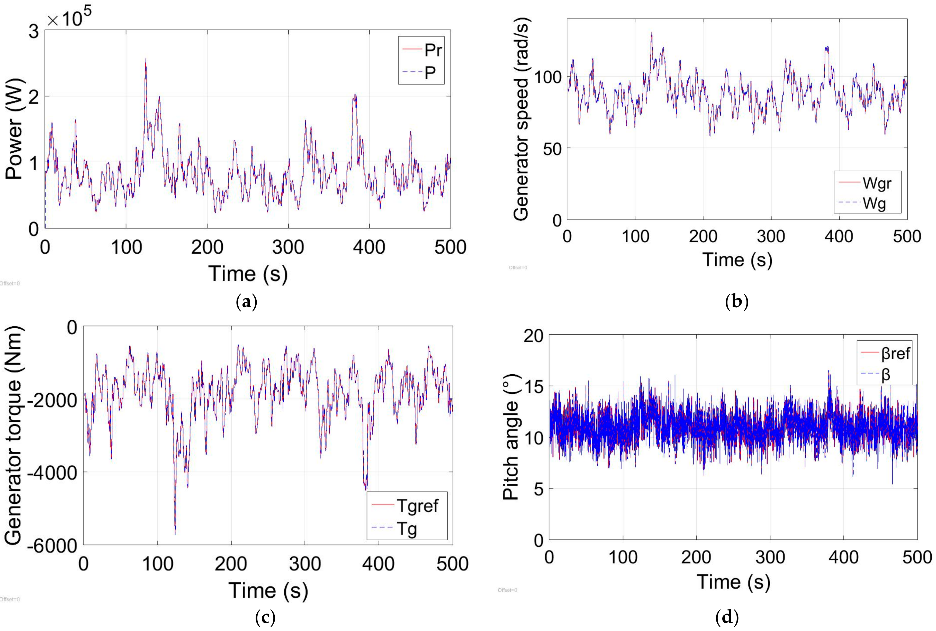
5.2. Wind Energy Conversion System Dynamic Value Tracking under Real-Time Wind
The maximum power reference can be obtained through look-up the table [49]. Given the best tip speed ratio , the generator speed reference can be calculated. With the expectation performance index (or CVaR, Min-Max), the proposed controller can calculate the real-time predictive control law.
Figure 8 shows the WECS maximum wind energy capture performance under real-time wind speed. All blue dotted lines are the outputs of WECS, and the red solid lines are references. When there is no system failure, the control performance of the proposed controller with CVaR and Min-Max are almost the same. And the tip speed ratio generally surrounds its optimal working point . The pitch angle and its fluctuation range are very small (within ), which is a reasonable range in the practical situations. The simulation results in Figure 8 suggest that the proposed scenario-based SMPC controller can track the maximum power set points well when the system is in the normal status.
5.3. Wind Energy Conversion SystemTracking Constant Value when Actuator Failure Probability is 5%, Gain Loss Γ = 0.8
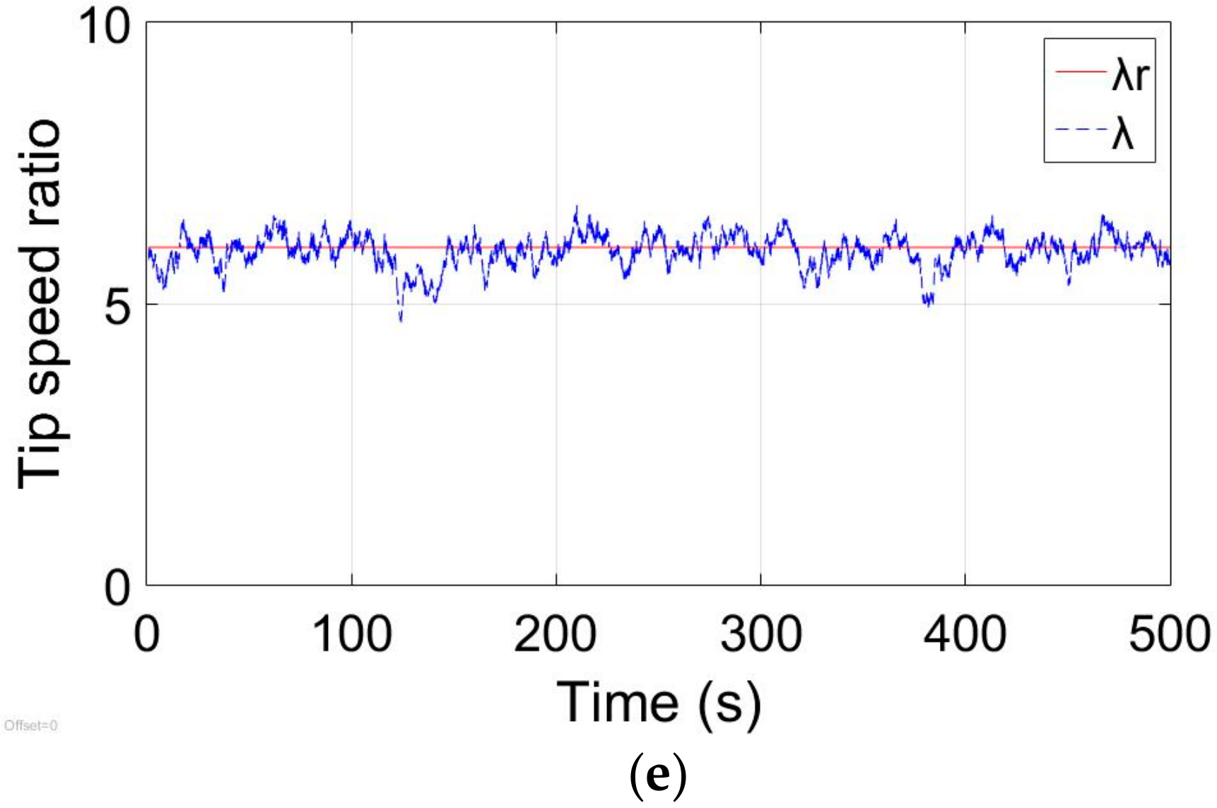
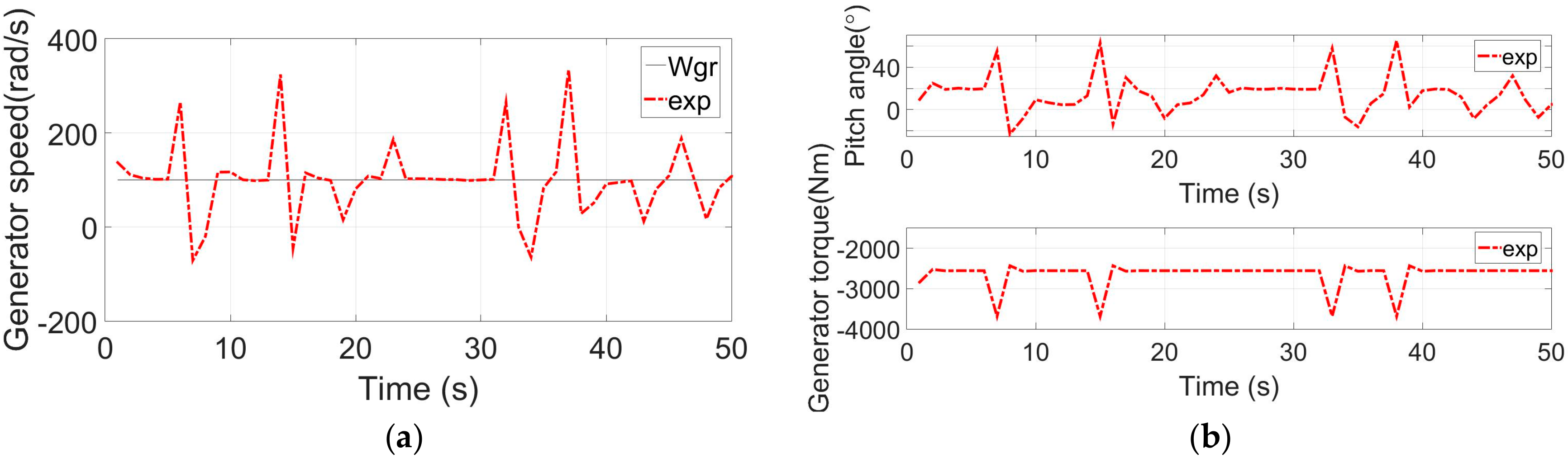
The purpose of this simulation is comparing the control performance of the SMPC controller with different objective functions with actuator fault. In this simulation, WECS actuator failure probability is set to 5% and gain loss is set to . Figure 9 gives the result of the proposed controller with expectation objective function. Figure 10 gives the result of the controller with the CVaR and the Min-Max objective function.
It can be observed from Figure 9 that the generator speed and the have been suffered in a bad situation under the control effort of the SMPC controller with the expectation objective function (some negative values even occurred during the control process). The input and output of the controller have obvious fluctuations, and the control performance is much worse than the proposed controller with the CVaR and Min-Max objective function (as shown in Figure 10). The simulation result indicates that the proposed controller with the expectation objective function has poor fault-tolerant control performance.
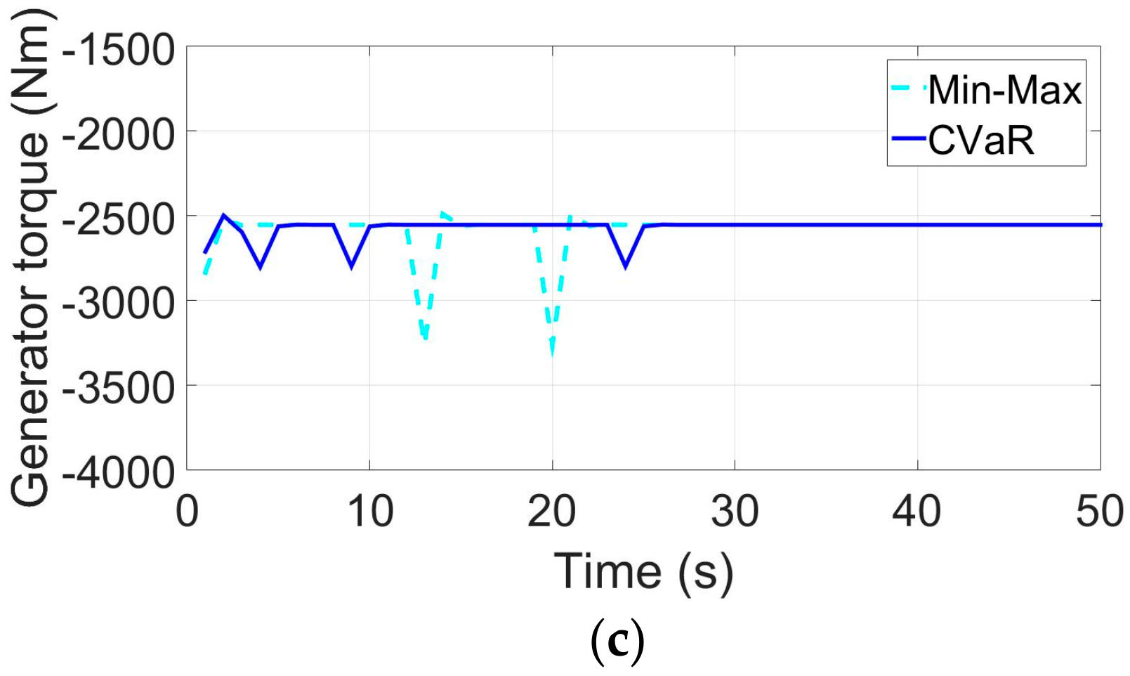
Figure 10 shows that the proposed controller with the CVaR or the Min-Max objective functions all have a good ability to address the actuator fault in the WECS. Meanwhile, the proposed controller with the CVaR objective function exhibits the best fault-tolerant control performance. It can maintain good fault-tolerant control performance when a probability 5% fault occurs in the WECS actuator. In Figure 10a, the fluctuation range of output generator speed is , which is smaller than the controller with the Min-Max objective function. This suggests that the controller with the CVaR objective function can track the power set points more precisely. In Figure 10b, the fluctuation range of pitch angle is in a reasonable range (about ); its fluctuations are not intense, which can reduce the loss of pitch systems. In Figure 10c, the generator torque reference under the controller with the CVaR objective function has minimum fluctuation amplitude, which can ensure the generator operates stably.
The simulation results above suggest that the CVaR is a good index of the SMPC fault-tolerant controller because this index can balance between the system risk and the control performance loss. Expectation objective functions are not suitable for fault-tolerant control problems, and the Min-Max control performance index suffers from heavy control performance loss, although its system risk is small. From the fluctuation range of the simulation results, the controller with the CVaR objective function is 40% less conservative than the one with the Min-Max objective function.
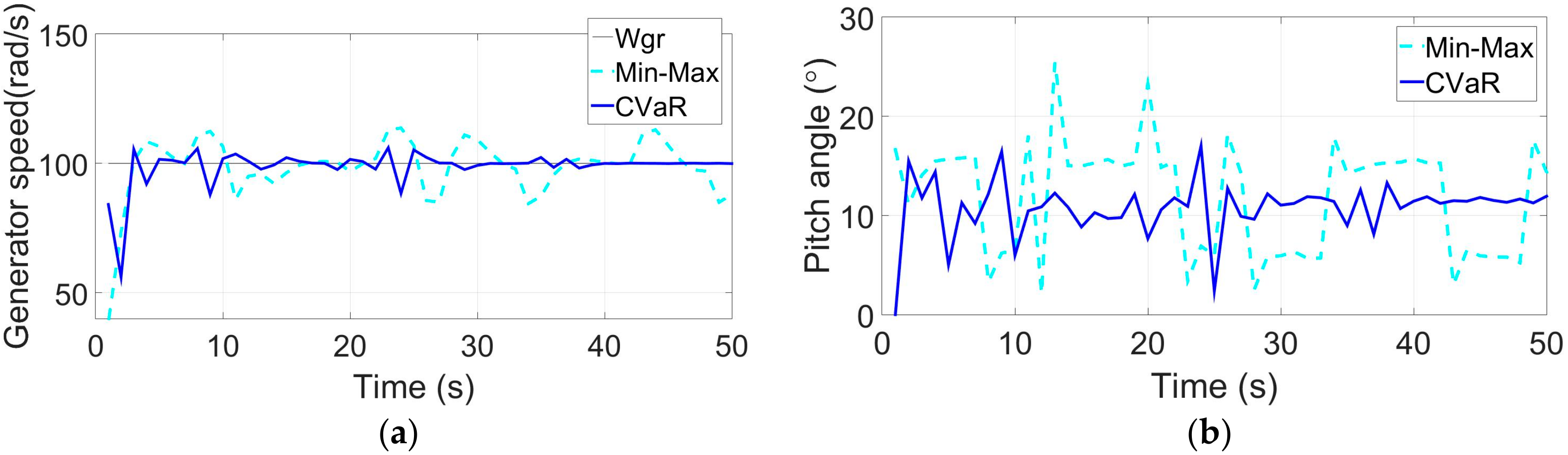
5.4. Wind Energy Conversion System Dynamic Value Tracking under Real-Time Wind when Actuator Failure Probability is 5%, Gain Loss Γ = 0.8
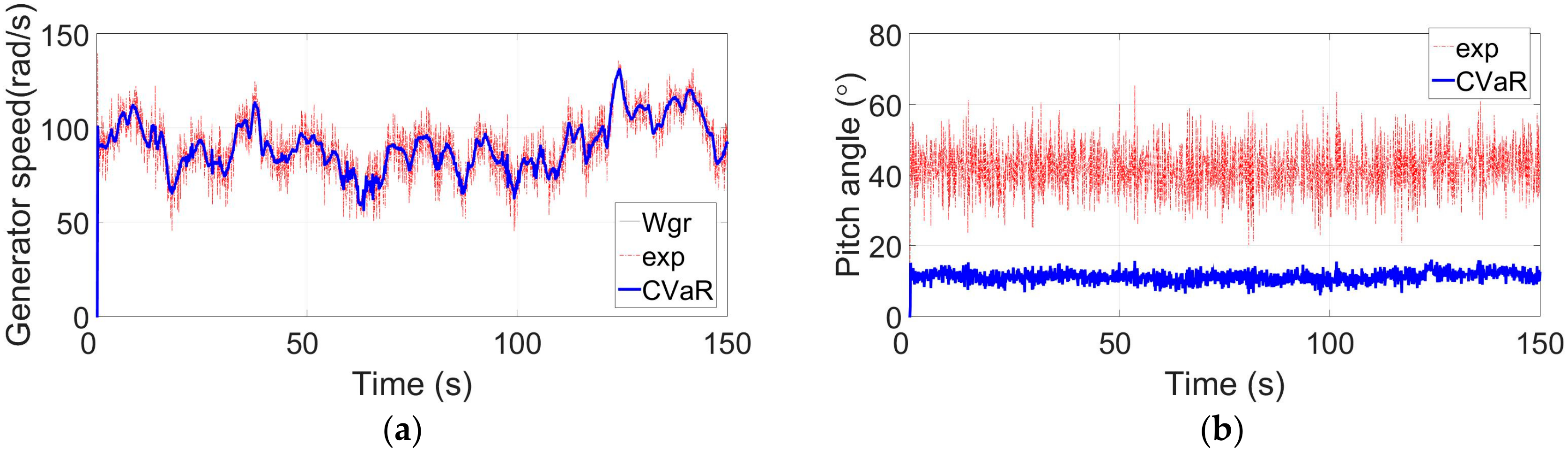
Figure 11 shows the control result of expectation and CVaR performance indexes when WECS actuator fails with probability 5%. In Figure 11, the CVaR has good dynamic fault-tolerant control performance and the expectation performance index behaves abnormally when the actuator fails with a probability of 5%. In Figure 11a, the controller with expectation performance index leads a large oscillation amplitude of the generator speed (about ±20 rad/s) and very high oscillation frequency. These issues will increase the mechanical losses of the pitch system. Notably, the CVaR tracks the dynamic references of generator speed very well. Its performance is slightly worse than the WECS under normal situation. In Figure 11b, the input pitch angle references under the controller with CVaR are in the normal range. However, the expectation objective function leads the input pitch angle reference deviating greatly from the normal range . These results suggest that the proposed controller with CVaR has better fault-tolerant control performance than the controller with expectation index.
6. Conclusions
WECSs are widely adopted to utilize wind energy. However, due to the randomness of the wind and the many nonlinear factors affecting the WECS, it is always necessary to guarantee the security and performance of the WECS under actuator faults. To solve the fault tolerance control problem of WECS with actuator probability faults, this paper proposes a scenario-based SMPC controller with the CVaR objective function. First, the Markov jump linear model of the wind turbine can be formulated with the help of the probability information of the wind. With this model, the randomness of the wind can be properly described. Notably, if the MPC controller is directly constructed with the Markov jump model, it will obtain an uncertain SMPC problem. For this reason, the proposed method uses scenario trees to formulate the probable states of the WECS under the wind. With the scenario trees, the uncertain SMPC problem is transformed into a deterministic MPC problem and the deterministic MPC problem can be more easily solved. Finally, the fault-tolerant controller is implemented using the CVaR performance index to punish excessive loss, which can provide a better balance between the system performance and failure risk. The simulation results show that the proposed SMPC with the CVaR objective function can solve the modeling and fault tolerance control problems of WECSs under actuator faults. Its control performance is 40% higher than the common Min-Max performance index. However, the proposed method has to solve the SMPC problem with the CVaR performance index in two steps. This is not the best solution. In the future, we’ll try to solve the SMPC problem with the CVaR objective function in one step, which will have a higher practical value.
Acknowledgments
This work is partly supported by the National Natural Science Foundation of China under Grant 61473002. The authors would like to thank Zhenwu Lei and Weichuan Liu for revising this paper.
Author Contributions
Yuntao Shi initiated and directed the study on the fault-tolerant control of WECS. Xiang Xiang designed the simulations, solved the SMPC fault-tolerant controller with the Conditional Value at Risk (CVaR) objective function. All authors performed the simulations, carried out data analysis, discussed the results and contributed to write the paper.
Conflicts of Interest
The authors declare no conflict of interest.
References
- Shehata, E.G. A comparative study of current control schemes for a direct-driven PMSG wind energy generation system. Electr. Power Syst. Res. 2017, 143, 197–205. [Google Scholar] [CrossRef]
- Jadhav, H.T.; Roy, R. A comprehensive review on the grid integration of doubly fed induction generator. Int. J. Electr. Power Energy Syst. 2013, 49, 8–18. [Google Scholar] [CrossRef]
- Spahic, E.; Underbrink, A.; Buchert, V.; Hanson, J.; Jeromin, I.; Balzer, G. Reliability model of large offshore wind farms. In Proceedings of the 2009 IEEE Bucharest PowerTech, Bucharest, Romania, 28 June–2 July 2009. [Google Scholar]
- Li, L.; You, S.; Yang, C.; Yan, B.; Song, J.; Chen, Z. Driving-behavior-aware stochastic model predictive control for plug-in hybrid electric buses. Appl. Energy 2016, 162, 868–879. [Google Scholar] [CrossRef]
- Di Cairano, S.; Bernardini, D.; Bemporad, A.; Kolmanovsky, I.V. Stochastic MPC with Learning for Driver-Predictive Vehicle Control and its Application to HEV Energy Management. IEEE Trans. Control Syst. Technol. 2014, 22, 1018–1031. [Google Scholar] [CrossRef]
- Velarde, P.; Valverde, L.; Maestre, J.M.; Ocampo-Martinez, C.; Bordonsa, C. On the comparison of stochastic model predictive control strategies applied to a hydrogen-based microgrid. J. Power Sources 2017, 343, 161–173. [Google Scholar] [CrossRef]
- Moser, D.; Schmied, R.; Waschl, H.; del Re, L. Flexible Spacing Adaptive Cruise Control Using Stochastic Model Predictive Control. IEEE Trans. Control Syst. Technol. 2017, 26, 114–127. [Google Scholar] [CrossRef]
- Raimondi Cominesi, S.; Farina, M.; Giulioni, L.; Picasso, B.; Scattolini, R. A Two-Layer Stochastic Model Predictive Control Scheme for Microgrids. IEEE Trans. Control Syst. Technol. 2017, 26, 1–13. [Google Scholar] [CrossRef]
- Parisio, A.; Rikos, E.; Glielmo, L. Stochastic model predictive control for economic/environmental operation management of microgrids: An experimental case study. J. Process Control 2016, 43, 24–37. [Google Scholar] [CrossRef]
- Bemporad, A.; Cairano, S.D. Model-Predictive Control of Discrete Hybrid Stochastic Automata. IEEE Trans. Autom. Control 2011, 56, 1307–1321. [Google Scholar] [CrossRef]
- Baloch, M.H.; Wang, J.; Kaloi, G.S. A review of the state of the art control techniques for wind energy conversion system. Int. J. Renew. Energy Res. 2016, 6, 1277–1295. [Google Scholar]
- Shahbazi, M.; Saadate, S.; Poure, P.; Zolghadri, M. Open-circuit switch fault tolerant wind energy conversion system based on six/five-leg reconfigurable converter. Electr. Power Syst. Res. 2016, 137, 104–112. [Google Scholar] [CrossRef] [Green Version]
- Lan, J.; Patton, R.J.; Zhu, X. Fault-tolerant wind turbine pitch control using adaptive sliding mode estimation. Renew. Energy 2016, 116, 219–231. [Google Scholar] [CrossRef]
- Schulte, H.; Gauterin, E. Fault-Tolerant Control of Wind Turbines with Hydrostatic Transmission using Takagi-Sugeno and Sliding Mode Techniques. Annu. Rev. Control 2015, 40, 82–92. [Google Scholar] [CrossRef]
- Shi, Y.T.; Kou, Q.; Sun, D.H.; Li, Z.X.; Qiao, S.J.; Hou, Y.J. H∞ Fault Tolerant Control of WECS Based on the PWA Model. Energies 2014, 7, 1750–1769. [Google Scholar] [CrossRef]
- Blesa, J.; Rotondo, D.; Puig, V.; Nejjari, F. FDI and FTC of wind turbines using the interval observer approach and virtual actuators/sensors. Control Eng. Pract. 2014, 24, 138–155. [Google Scholar] [CrossRef]
- Gonçalves, P.F.C.; Cruz, S.M.A.; Abadi, M.B.; Caseiro, L.M.A.; Mendes, A.M.S. Fault-tolerant predictive power control of a DFIG for wind energy applications. IET Electr. Power Appl. 2017, 11, 969–980. [Google Scholar] [CrossRef]
- Sellami, T.; Berriri, H.; Jelassi, S.; Darcherif, A.M.; Mimouni, M.F. Short-Circuit Fault Tolerant Control of a Wind Turbine Driven Induction Generator Based on Sliding Mode Observers. Energies 2017, 10, 1611. [Google Scholar] [CrossRef]
- Lin, Z.; Liu, J.; Wu, Q.; Niu, Y. Mixed H2/H∞ Pitch Control of Wind Turbine with a Markovian Jump Model. Int. J. Control 2016, 91, 156–169. [Google Scholar] [CrossRef]
- Sloth, C.; Esbensen, T.; Stoustrup, J. Robust and fault-tolerant linear parameter-varying control of wind turbines. Mechatronics 2011, 21, 645–659. [Google Scholar] [CrossRef]
- Camacho, E.F.; Alamo, T.; Peña, D.M.D.L. Fault-tolerant model predictive control. In Proceedings of the 2010 IEEE Conference On Emerging Technologies and Factory Automation, Bilbao, Spain, 13–16 September 2010. [Google Scholar]
- Patwardhan, S.C.; Manuja, S.; Narasimhan, S.; Shah, S.L. From data to diagnosis and control using generalized orthonormal basis filters. Part II: Model predictive and fault tolerant control. J. Process Control 2006, 16, 157–175. [Google Scholar] [CrossRef]
- Rodil, S.S.; Fuente, M.J. Fault tolerance in the framework of support vector machines based model predictive control. Eng. Appl. Artif. Intell. 2010, 23, 1127–1139. [Google Scholar] [CrossRef]
- Almeida, F.D.; Leissling, D. Fault-Tolerant Model Predictive Control with Flight Test Results on ATTAS. Eng. Appl. Artif. Intell. 2013, 33, 363–375. [Google Scholar]
- Kale, M.M.; Chipperfield, A.J. Stabilized MPC formulation for robust reconfigurable flight control. Control Eng. Pract. 2005, 13, 771–788. [Google Scholar] [CrossRef]
- Ocampo-Martinez, C.; Puig, V.; Quevedo, J.; Ingimundarson, A. Fault Tolerant Model Predictive Control applied on the Barcelona Sewer Network. In Proceedings of the 44th IEEE Conference on Decision and Control, 2005 and 2005 European Control Conference (CDC-ECC ’05), Seville, Spain, 12–15 December 2005; IEEE: Piscataway, NJ, USA, 2006; pp. 1349–1354. [Google Scholar]
- Hartley, E.N.; Maciejowski, J.M. A longitudinal flight control law based on robust MPC and H2 methods to accommodate sensor loss in the RECONFIGURE benchmark. IFAC PapersOnline 2015, 48, 1000–1005. [Google Scholar] [CrossRef] [Green Version]
- Maciejowski, J.M.; Yang, X. Fault tolerant control using Gaussian processes and model predictive control. In Proceedings of the 2013 Conference on Control and Fault-Tolerant Systems, Nice, France, 9–11 October 2013; IEEE: Piscataway, NJ, USA, 2015; pp. 1–12. [Google Scholar]
- Rockafellar, R.T.; Uryasev, S. Optimization of Conditional Value-At-Risk. J. Risk 2000, 29, 1071–1074. [Google Scholar] [CrossRef]
- Capiński, M.J. Hedging Conditional Value at Risk with options. Eur. J. Oper. Res. 2015, 242, 688–691. [Google Scholar] [CrossRef]
- Hosseini-Firouz, M. Optimal offering strategy considering the risk management for wind power producers in electricity market. Int. J. Electr. Power Energy Syst. 2013, 49, 359–368. [Google Scholar] [CrossRef]
- Kothare, M.V.; Balakrishnan, V.; Morari, M. Robust constrained model predictive control using linear matrix inequalities. In Proceedings of the 1994 American Control Conference, Baltimore, MD, USA, 29 June–1 July 1994; IEEE: Piscataway, NJ, USA, 2002; Volume 1, pp. 440–444. [Google Scholar]
- Song, Z.; Geng, X.; Kusiak, A.; Xu, C. Mining Markov chain transition matrix from wind speed time series data. Expert Syst. Appl. 2011, 38, 10229–10239. [Google Scholar] [CrossRef]
- Ross, S.M. Introduction to Probability Models, 1st ed.; Elsevier: New York, NY, USA, 2007. [Google Scholar]
- Zitzler, E.; Laumanns, M.; Thiele, L. SPEA2: Improving the Strength Pareto Evolutionary Algorithm; ETH Library: Zürich, Switzerland, 2001. [Google Scholar]
- Zitzler, E.; Thiele, L. Multiobjective evolutionary algorithms: A comparative case study and the strength Pareto approach. IEEE Trans. Evol. Comput. 1999, 3, 257–271. [Google Scholar] [CrossRef]
- Esbensen, T.; Sloth, C. Fault Diagnosis and Fault-Tolerant Control of Wind Turbine; Aalborg University: Aalborg, Denmark, 2009. [Google Scholar]
- Højstrup, J. Velocity spectra in the unstable planetary boundary layer. J. Atmos. Sci. 1982, 39, 2239–2248. [Google Scholar] [CrossRef]
- Østergaard, K.Z.; Brath, P.; Stoustrup, J. Estimation of effective wind speed. J. Phys. 2007, 75, 1–9. [Google Scholar] [CrossRef]
- Burkart, R.; Margellos, K.; Lygeros, J. Nonlinear control of wind turbines: An approach based on switched linear systems and feedback linearization. In Proceedings of the 2011 50th IEEE Conference on Decision and Control and European Control Conference, Orlando, FL, USA, 12–15 December 2011; IEEE: Piscataway, NJ, USA, 2011; pp. 5485–5490. [Google Scholar]
- Bryson, A.E. Applied Linear Optimal Control: Examples and Alogrithms; Cambridge University Press: Cambridge, UK, 2002. [Google Scholar]
- Bernardini, D.; Bemporad, A. Stabilizing Model Predictive Control of Stochastic Constrained Linear Systems. IEEE Trans. Autom. Control 2012, 57, 1468–1480. [Google Scholar] [CrossRef]
- Pena, D.M.D.L.; Alamo, T.; Bemporad, A.; Camacho, E.F. Feedback min-max model predictive control based on a quadratic cost function. In Proceedings of the 2006 American Control Conference, Minneapolis, MN, USA, 14–16 June 2006. [Google Scholar]
- Andersen, T.; Bollerslev, T. Volatility and correlation forecasting. In Handbook of Economic Forecasting; Elsevier: New York, NY, USA, 2006; Volume 1, pp. 777–878. [Google Scholar]
- Escanciano, J.C.; Pei, P. Pitfalls in backtesting Historical Simulation VaR models. J. Bank. Financ. 2012, 36, 2233–2244. [Google Scholar] [CrossRef]
- Bemporad, A.; Puglia, L.; Gabbriellini, T. A stochastic model predictive control approach to dynamic option hedging with transaction costs. In Proceedings of the American Control Conference, San Francisco, CA, USA, 29 June–1 July 2011. [Google Scholar]
- Camacho, E.F.; Bordons, C. Model Predictive Control; Springer: Berlin, Germany, 1999. [Google Scholar]
- Kwakernaak, H.R. Linear Optimal Control Systems; Wiley: Hoboken, NJ, USA, 1972. [Google Scholar]
- Munteanu, I. Optimal Control of Wind Energy Systems; Springer: Berlin, Germany, 2008. [Google Scholar]
Figure 1.
(a) Wind speed; (b) Wind speed and the corresponding working point.

Figure 2.
The structure of wind energy conversion system.
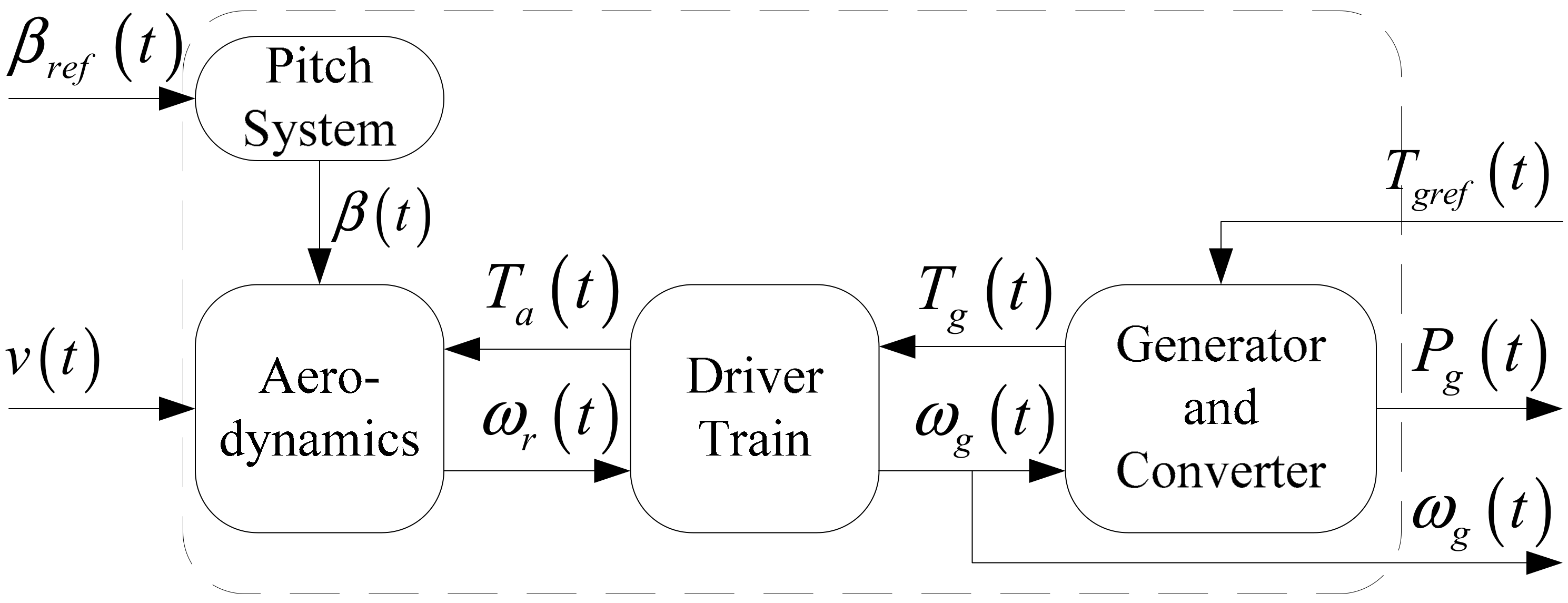
Figure 3.
Scenario tree with root node .

Figure 4.
The relationship of the system performance and risk.

Figure 5.
probability density.
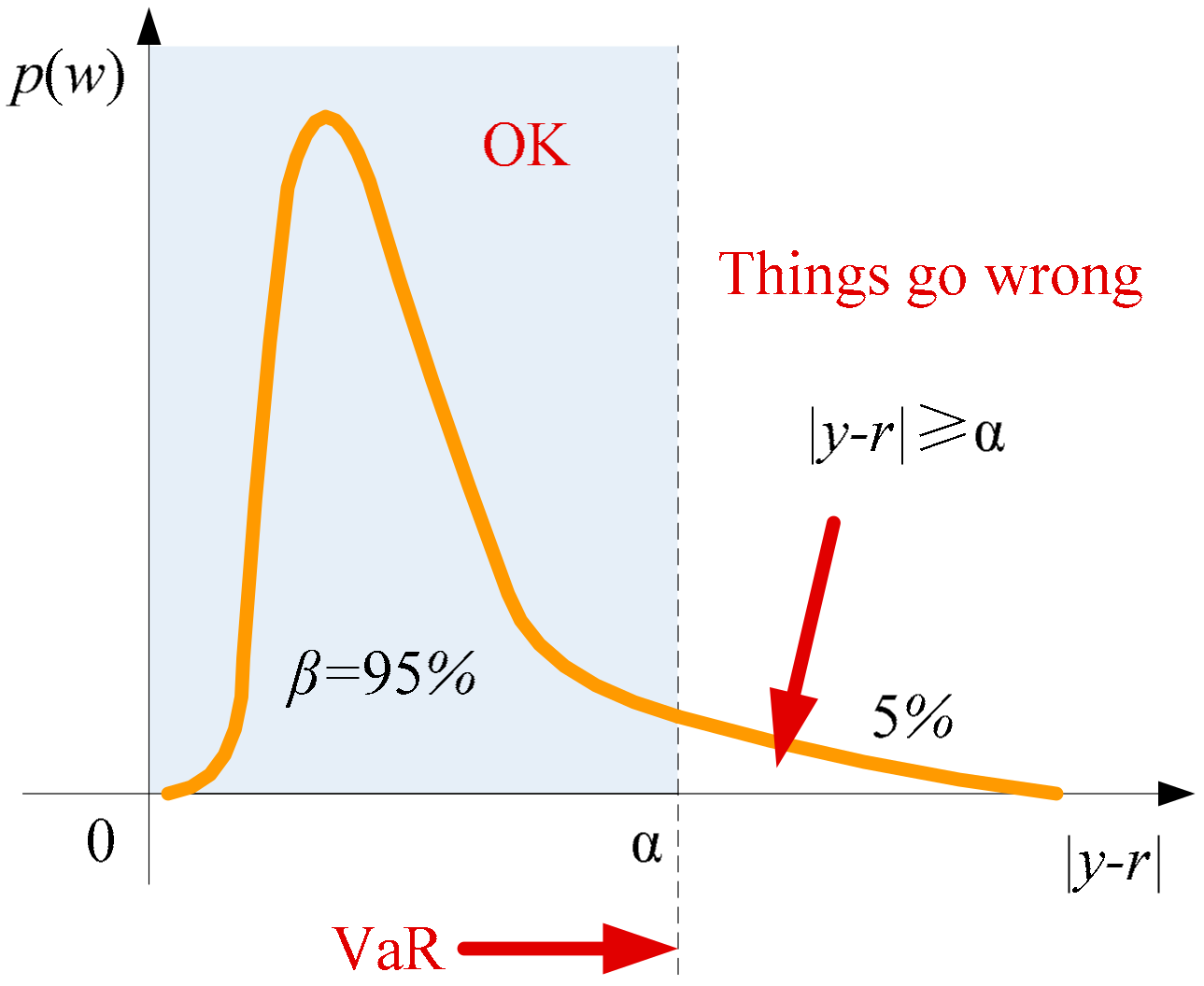
Figure 6.
Power error probability density.

Figure 7.
This figure shows the WECS output and input of constant power tracking with three objective function (Exp, CVaR, Min-Max): (a) Output generator speed tracking set points; (b) input pitch angle reference; (c) input generator torque reference .
Figure 7.
This figure shows the WECS output and input of constant power tracking with three objective function (Exp, CVaR, Min-Max): (a) Output generator speed tracking set points; (b) input pitch angle reference; (c) input generator torque reference .
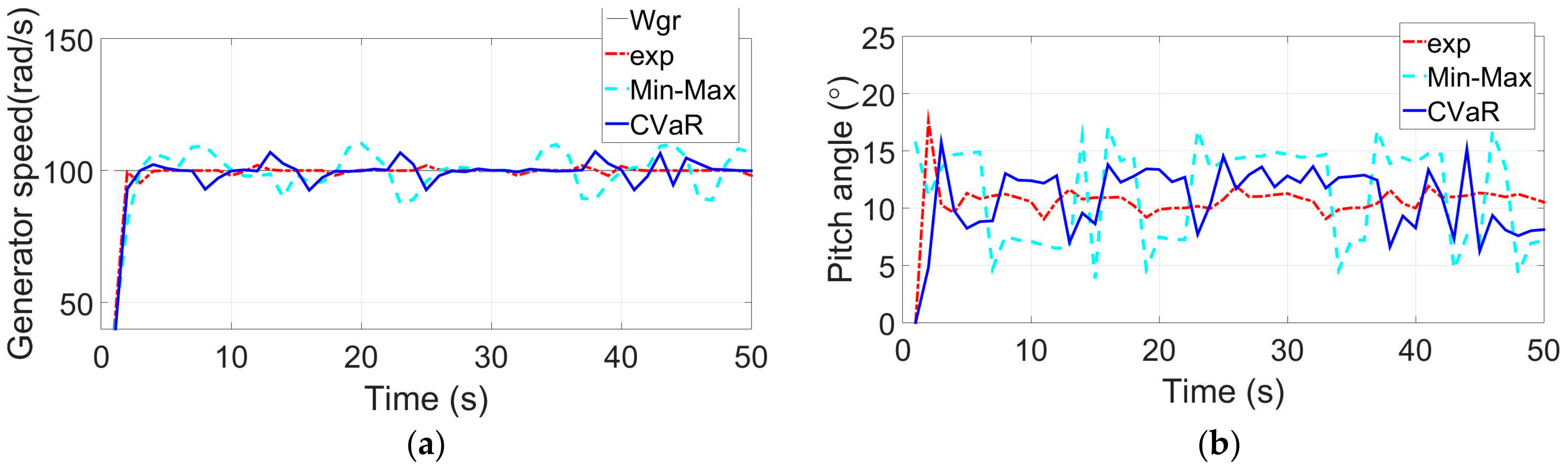

Figure 8.
WECS maximum wind energy capture under real-time wind: (a) Maximum power tracking; (b) Generator speed tracking; (c) Generator torque tracking; (d) Pitch angle tracking; (e) Tip speed ratio tracking.
Figure 8.
WECS maximum wind energy capture under real-time wind: (a) Maximum power tracking; (b) Generator speed tracking; (c) Generator torque tracking; (d) Pitch angle tracking; (e) Tip speed ratio tracking.


Figure 9.
The output and input when WECS under the control of expectation performance index, actuator failure probability is 5%, gain loss is : (a) Output generator speed ; (b) input generator torque reference and pitch angle reference .
Figure 9.
The output and input when WECS under the control of expectation performance index, actuator failure probability is 5%, gain loss is : (a) Output generator speed ; (b) input generator torque reference and pitch angle reference .

Figure 10.
The output and input when WECS under the control of CVaR, Min-Max objective functions, actuator failure probability is 5%, gain loss is : (a) Output generator speed ; (b) pitch angle reference ; (c) input generator torque reference .
Figure 10.
The output and input when WECS under the control of CVaR, Min-Max objective functions, actuator failure probability is 5%, gain loss is : (a) Output generator speed ; (b) pitch angle reference ; (c) input generator torque reference .


Figure 11.
The control result of expectation and CVaR performance indexes when WECS actuator fails with probability 5%, gain loss : (a) Output generator speed ; (b) Input pitch angle reference .
Figure 11.
The control result of expectation and CVaR performance indexes when WECS actuator fails with probability 5%, gain loss : (a) Output generator speed ; (b) Input pitch angle reference .


Table 1.
Parameters of linearized model in different working points.
| Parameters | ||||||
|---|---|---|---|---|---|---|
| a84 | a88 | e81 | a1 | a2 | a3 | |
| 0.409 | 0.50 | 1.90 | 0.3125 | 2.92 | 0.9375 | |
| 0.479 | 0.53 | 2.31 | 0.33 | 3.65 | 2.3 | |
| 0.833 | 0.53 | 2.50 | 0.625 | 5 | 5 | |
Table 2.
Gain loss.
| Loss of Gain | Fault Degree | ||
|---|---|---|---|
| 1 | 0 | ||
| actuator | normal | partial loss | complete failure |
© 2018 by the authors. Licensee MDPI, Basel, Switzerland. This article is an open access article distributed under the terms and conditions of the Creative Commons Attribution (CC BY) license (http://creativecommons.org/licenses/by/4.0/).
Share and Cite
MDPI and ACS Style
Shi, Y.-T.; Xiang, X.; Wang, L.; Zhang, Y.; Sun, D.-H. Stochastic Model Predictive Fault Tolerant Control Based on Conditional Value at Risk for Wind Energy Conversion System. Energies 2018, 11, 193. https://doi.org/10.3390/en11010193
AMA Style
Shi Y-T, Xiang X, Wang L, Zhang Y, Sun D-H. Stochastic Model Predictive Fault Tolerant Control Based on Conditional Value at Risk for Wind Energy Conversion System. Energies. 2018; 11(1):193. https://doi.org/10.3390/en11010193
Chicago/Turabian StyleShi, Yun-Tao, Xiang Xiang, Li Wang, Yuan Zhang, and De-Hui Sun. 2018. "Stochastic Model Predictive Fault Tolerant Control Based on Conditional Value at Risk for Wind Energy Conversion System" Energies 11, no. 1: 193. https://doi.org/10.3390/en11010193
Note that from the first issue of 2016, this journal uses article numbers instead of page numbers. See further details here.