The Energy Saving Potential of Occupancy-Based Lighting Control Strategies in Open-Plan Offices: The Influence of Occupancy Patterns


Building Lighting Group, Department of the Built Environment, Technical University Eindhoven, Groene Loper 6, 5600 MB Eindhoven, The Netherlands
*
Author to whom correspondence should be addressed.
Energies 2018, 11(1), 2; https://doi.org/10.3390/en11010002
Submission received: 27 October 2017
/
Revised: 4 December 2017
/
Accepted: 18 December 2017
/
Published: 21 December 2017
(This article belongs to the Special Issue Smart Lighting Environments: Sensing and Control)
Abstract
:Occupancy-based lighting control strategies have been proven to be effective in diminishing offices’ energy consumption. These strategies have typically worked by controlling lighting at the room level but, recently, lighting systems have begun to be equipped with sensors on a more fine-grained level, enabling lighting control at the desk level. For some office cases, however, the savings gained using this strategy may not outweigh the costs and design efforts compared to room control. This is because, in some offices, individual occupancy patterns are similar, hence the difference in savings between desk and room control would be minimal. This study examined the influence of occupancy pattern variance within an office space on the relative energy savings of control strategies with different control zone sizes. We applied stochastic modeling to estimate the occupancy patterns, as this method can account for uncertainty. To validate our model, simulation results were compared to earlier studies and real measurements, which demonstrated that our simulations provided realistic occupancy patterns. Next, office cases varying in both job-function type distribution and office policy were investigated on energy savings potential to determine the influence of occupancy pattern variance. The relative energy savings potential of the different control strategies differed minimally for the test cases, suggesting that variations in individual occupancy patterns negligibly influence energy savings. In all cases, lighting control at the desk level showed a significantly higher energy savings potential than strategies with lower control zone granularity, suggesting that it is useful to implement occupancy-based lighting at the desk level in all office cases. This strategy should, thus, receive more attention from both researchers and lighting designers.
1. Introduction
Office building energy consumption has long received attention from researchers, but it has become a necessity since the European Commission formulated the goal of diminishing its CO2 emissions by 80% by the year 2050 [1]. This goal requires a decrease in energy consumption in all cases. Artificial lighting still comprises about 5–15% of the total energy consumption of offices [2]; this is the case even with recent developments in lighting technologies, such as solid-state lighting [3].
Yet, advances are being made. In addition to new lighting sources, automatic lighting control strategies are being applied to provide lighting based on the real-time needs of offices [4]. The main variables determining these needs are (1) the availability of daylight, and (2) the presence of occupants in an office space. These factors can be determined with light and occupancy sensors, respectively. Occupancy sensors have been applied for many years in offices and have been proven to produce energy savings of between 20% and 60% [5,6,7]. However, to achieve maximal energy savings, occupancy sensors should be combined with daylight controls [8,9].
Currently, lighting systems are increasingly applying smart technology by using occupancy sensors that enable smaller control zones (higher granularity) compared to traditional systems with global presence detection [10,11,12]. With these smaller control zones, lighting is used optimally, since it is tailored to the occupancy patterns of individuals. In North America, two studies have evaluated lighting control at the desk level on energy savings potential [6,13], finding that the relative savings were 42% and 40% compared to baseline cases, where, respectively, lighting was used according to the daily work schedule and where lighting was switched on and off manually [6,13]. Additionally, several other studies have investigated the energy savings potential of occupancy-based lighting control, but always for specific office cases (e.g., [7,14]). Consequently, as discussed by Chew et al. [12], the results differed greatly. This might have been due to the job-function types of the occupants—their occupation, e.g., secretary or manager—differing across the studies; research found that, among other factors, job-function type caused occupancy patterns to differ [15,16]. Chang et al. [17] showed that users’ occupancy patterns could be categorized into five different types, and argued that job characteristics are likely to underlie these distinct types. Hence, for office cases with occupants who differ in function type, energy savings might deviate from the numbers found by [6,13]. Even more importantly, lighting control at the desk level might not be useful to implement. Instead, in certain cases, it is just as efficient to control the lighting by larger control zones, e.g., by subgroup or room. For example, in office spaces where all occupants have the same function type, and, thus, highly similar occupancy patterns, lighting control at the desk level might not result in significantly higher energy savings compared to control at the room level. To investigate this further, this study focused on the influence of occupancy pattern variance on relative energy savings of various lighting control strategies that differed in control zone granularity.
In their work, Chew et al. [12] argued that the variations in the reported results on energy savings from occupancy-based lighting control might impede widespread implementation of smart lighting, in part, because of its generally high installation costs. Therefore, it is important to determine the mixtures of office employees where fine-grained lighting control will outweigh the costs of installation. More specifically, for current office buildings, it is key to compare fine-grained occupancy-based lighting control to the strategies with larger control zones, as these offices are rarely equipped with fine-grained sensor networks. However, even in those cases when such a sensor network is present, control at a granularity level lower than the desk level might be preferred; at the desk level, additional design and assessment efforts are required to assure compliance with regulations. In contrast to room control, where lighting conditions remain constant throughout space and time, control at the desk level results in dynamic lighting. This might affect the comfort of users, specifically for open-plan offices during times of limited occupancy; in these offices, users are able to see the entire workspace, in contrast to the more obstructed views of cubicle offices [18]. As a result, a sudden change in illuminance or reduced background illuminance may cause discomfort or reduce task performance [4]. This discomfort might be overcome by dimming the lighting only to certain levels and by using a dimming speed that makes changes imperceptible to occupants [19]. This provides another reason for utilizing highly granular lighting control only when it results in a significant reduction of an office’s energy consumption.
Recent studies have compared the potential energy savings of occupancy-based lighting control to other lighting control strategies—for example, to daylight dimming [20], time scheduling [21], and personal control [6]. However, this research did not examine potential energy savings of control strategies that differed in zone granularity, which further increases the significance of this study. Researchers have investigated the zone control strategy at just one control zone size, e.g., a subgroup of desks [14] or at individual desks [22]. Additionally, the influence of control settings on potential energy savings has also been studied, e.g., the effect of a time delay setting [5]. However, as far as we know, no work has examined the influence of zone granularity.
In our investigation, simulations were performed for office cases that differed on two factors: (1) office policy, and (2) function type distribution. Both of these factors can affect occupancy pattern variations in office spaces. In our work, the energy savings of occupancy-based lighting control was calculated in three different control zone sizes—room, subgroup, and desk level—and compared to a manual control baseline case. From this, it could be determined whether occupancy pattern variations caused variances in energy savings across the three zone control sizes, and more specifically, which control zone size provided the greatest degree of energy savings for the different office cases.
This paper describes how we developed the model and then presents the results from a first validation study and those from simulations for fictive office cases that differed depending on (1) the office policy, and (2) the function type distribution.
2. Methodology
In Section 2.1, we first explain the modeling techniques that we used, and then we elaborate on the four different steps of the model successively. In Section 2.2, we describe the simulations that we performed to validate the model and we discuss the office cases that were tested to determine the influence of (1) function type distribution; and (2) office policy.
2.1. The Model
2.1.1. Modeling Techniques
In line with recent studies investigating occupancy behavior [23], we applied a stochastic modeling approach. Building energy simulations (BESs), such as the ASHRAE 90.1-2013 occupancy profiles, have used homogenous profiles [24,25]; however, as these profiles do not account for the stochastic characteristic of human behavior [26,27], research has moved away from this method, and has taken up stochastic modeling. As the stochastic modeling technique randomizes events, it makes it possible to include a reasonable estimation of real-life variance.
In stochastic modeling, multiple iterations are performed to converge to an average, representative solution. In our examination, one iteration involved a full day of occupancy behavior at a one-minute time interval, i.e., whether the occupants were present or absent for each minute of the workday—a shorter time interval would have been impractical.
The parameters defining the office policy and function distribution of the office case at hand were included through agent-based modeling [28], as this method was expected to increase the prediction accuracy of the occupants’ behavior. For office cases where these parameters were missing, a standard set of averaged data was used as the inputs. We utilized MATLAB (The MathWorks, Inc., Natick, MA, USA) to create the white box model.
As illustrated in Figure 1, the model consisted of four major parts, each of which will be explained in the following sections.
2.1.2. Model Setup
The model consisted of five categories of input parameters that had to be set for the specific office case before simulations could be performed. Table 1 provides an overview of these parameters. Four categories of parameters were created that affected the presence of employees in the office, while the fifth category determines the energy use of the lighting control strategy. In this study, the parameters of the categories “function type” and “office policy” were varied as they were of main interest; in Section 2.2.2, we explain at which values of these parameters simulations were performed. The parameters of the other three categories were constant across simulations; their values will be described in this section.
Job-Function Type
First of all, each individual was assigned a job-function type. Eight different job-function types were pre-defined to enhance the utility of our model: Secretary, Manager, Drafter, Designer, Helpdesk employee, Team leader, Sales representative, and Consultant. The types differed by the number and length of absence events. For example, as Sales representatives often have to visit clients, they are likely to be absent more often and for longer periods in contrast to, for example, Helpdesk employees, who often sit behind their desks all day. We differed their daily average number of absence events for seven different duration categories: 1–5, 5–15, 15–30, 30–60, 60–90, 90–120, and 120–240 min (see Table 2). The absence events could occur at three moments during the day—morning, lunch, or afternoon—and their lengths were randomized at each iteration, within the category limits using a one-minute interval. The number of the absence events was also randomized, so that the long-term average would conform to the value set for a particular job-function type. No other parameters required randomization, as they did not vary over the course of a day.
Special Absences
The second category, “special absences”, was created because the number of holidays, for example, can also vary between employees. By including the parameter the full-time equivalent (FTE), the model could define how many hours an occupant works per week; this aspect needed to be included because it causes absences when the number of hours is less than a full work week. We set the number of holidays at 25 per year, the chance of a sick day at 0.02 and the FTE at 1. These values were chosen to represent a typical Dutch office; they were all based on government data (SCP, 2013).
Office Policy
Thirdly, the category “office policy” included parameters defining how much flexibility a company grants to his employees regarding working times, e.g., allowed start time and lunch length. Some occupants lunch at their desks, therefore, the lower limit of the lunch duration was set to 0 min.
Absence Type
When occupants within the office space had the same job-function type, they were modeled to attend group meetings together, just as occurs in a real office environment. To account for the ratio between group and individual absence events, we included the category “absence type”. We set its value at 0.5 for all job-function types, as we had no prior knowledge on which to base this value.
Lighting System Settings
The fifth category comprised of the settings of the lighting system. First of all, all simulations were performed for a fictive office consisting of 16 desks, each equipped with their own occupancy sensor and LED luminaire. We used a dimming level of 0.2 and activity timer of 15 min in all simulations. This means that in the case of control zone vacancies, luminaires in the zone were dimmed to 20% of their power 15 min after a vacancy was detected, as this is the time delay setting typically used in offices. The 20% setting was chosen so that a horizontal illuminance of approximately 100 lx would be maintained in background areas for the remaining occupants, as recommended by the European lighting standard EN 12464-1 [29]. Additionally, this percentage was also chosen because office luminaires are typically designed to provide 500 lx horizontally on desk areas when fully-switched on. The norm also recommends 300 lx horizontally in the surrounding area; as this surrounding area is defined as a band of 0.1 m around the task area, this illuminance level is likely to be achieved by the fully-switched on luminaire above the desk of the present occupant.
As explained in the Introduction, the goal was to compare the lighting energy use of control strategies differing on the degree of control zoning. Hence, the control zone size was set at 1 for individual control, 2, 4, and 8 for subgroup control, and 16 for room control. This means that when an occupant was present within the control zone, all luminaires in the zone were switched on, but they were only switched off when all occupants had left the control zone. With subgroup control, occupants with the same job-function type (see Table 2) were placed in the same zone, as this would provide the most energy-efficient lighting use.
As the aim of this study was to provide a first estimation of the lighting energy use of a particular office workspace, advanced lighting needs that come into play when considering the whole building were not taken into account. For example, the need for aisles to remain lit until the last person leaves the office was not taken into account in the energy calculations. In addition, the control algorithm did not take into account of daylight availability because this would highly complicate the calculations while we were interested in the relative energy saving potential of occupancy-based lighting control strategies.
2.1.3. Occupancy Generation
After the input parameters were set, the occupancy behavior could be generated. First, the model determined whether a special absence event had occurred (as mentioned in Table 1), as this would mean that an occupant was absent the whole day. If not, the daily occupancy behavior of the individuals was generated in four steps: (1) start and end time; (2) lunch-break absence; (3) individual absence events; and (4) group absence events (see Figure 2). The group absence events were not created individually, but for each function type and were included in the occupancy patterns of each occupant assigned to that function type. The model also generated standard deviations and anticipated minimum and maximum values for each iteration, allowing for an analysis of the spread and the robustness of a specific scenario.
2.1.4. Data Aggregation
The resulting individual occupancy patterns and their statistics were aggregated in a matrix with each iteration. Consequently, the daily lighting energy use was calculated for the three occupancy-based lighting control strategies using the following formula:
During the time that any of the occupants within the zone was present, lighting was switched on fully, thus multiplied by 1; during total absences, it was dimmed to 0.2, as explained in Section 2.1.2. The total number of minutes that the workday compromised was calculated from the moment that the first occupant arrived in the office until the time that the latest occupant left the office; it varied per iteration due to the variable start time of the last occupant. The maximum lighting energy use of 1 occurred when the first occupant arrived at the earliest time possible and the last occupant left at the latest time possible. We then took the average of lighting energy usages over the 1000 iterations; hence, the value of the lighting energy use was always lower than 1.
In addition, we calculated their energy saving potential compared to central manual control to determine the relevance of implementing the different types of occupancy-based lighting control for the office test cases. With central manual control, all luminaires are switched on by the first occupant arriving in the morning and switched off by the last person leaving. In our model, it was assumed that occupants always performed these actions, regardless of, for example, the availability of daylight. Between the start-of-the-day and end-of-the-day times, it was assumed that all lighting remained switched on. We felt that this provided a more realistic comparison baseline than, for example, scheduled switching.
The occupancy pattern variation, our second variable of interest in addition to energy use, was presented by the variable “relative spread”—or variance—between the individual occupancy patterns in the office space (range = 0–1). By “individual occupancy patterns,” we are referring to the occupancy states (thus, present or absent) of an individual over a day. We performed several calculations to determine the relative spread.
First, we calculated the real-time room occupancy (OccRT) and the mean room occupancy over the course of a day (OccMean). The room occupancy comprised the occupancy rate of the room (range = 0–1). For example, when five of the 12 occupants were present, the room occupancy would have been 0.417. The difference between OccRT and OccMean was defined as the real-time spread (SpreadRT) between the individual occupancy patterns. The spread between the individual occupancy patterns was maximal when OccRT was equal to OccMean, as this would mean that the variance in individual occupancy states (present or absent) was as large as possible while still resulting in the same average occupancy that was simulated, thus when 50% of the room was occupied. In a space that has an average room occupancy of 80%, periods of 50% real-time occupancy must be compensated for with periods of real-time occupancy >80%, as the room would be almost entirely occupied at this occupancy rate, resulting in periods of low spread. The absolute spread only provides information on the deviation of the spread from 50% occupancy, and this makes the spread highly dependent of the average occupancy. Therefore, we chose to calculate the relative spread—the deviation from the average occupancy—instead of the absolute spread. The spread was minimal (SpreadMin) when the real-time occupancy deviated maximally from the mean occupancy. This would mean that all occupants always arrived and left at the same time. In the example of an average room occupancy of 80%, the occupancy of the room would be 100% for 80% of the time and 0% for 20% of the time to achieve the minimal spread. A representation of this value for the minimum spread is found by the following equation:
The real-time spread (SpreadRT) is calculated as follows:
Finally, the average daily value for the spread relative to the minimal spread provides the relative spread (0–1) between the individual occupancy patterns for the whole iteration:
2.1.5. Data Presentation
During this last step, graphs were generated showing the simulated minimum and maximum values of the real-time room occupancy for a single day, the average room occupancy pattern, and its standard deviation. These were used as a basis for the graphs required to answer our research questions, which will be explained in Section 2.2.2. In Section 2.2.1, we first explain which calculations were made and which graphs were plotted to validate our model.
2.2. Simulations
2.2.1. Validating the Model
Occupancy Patterns
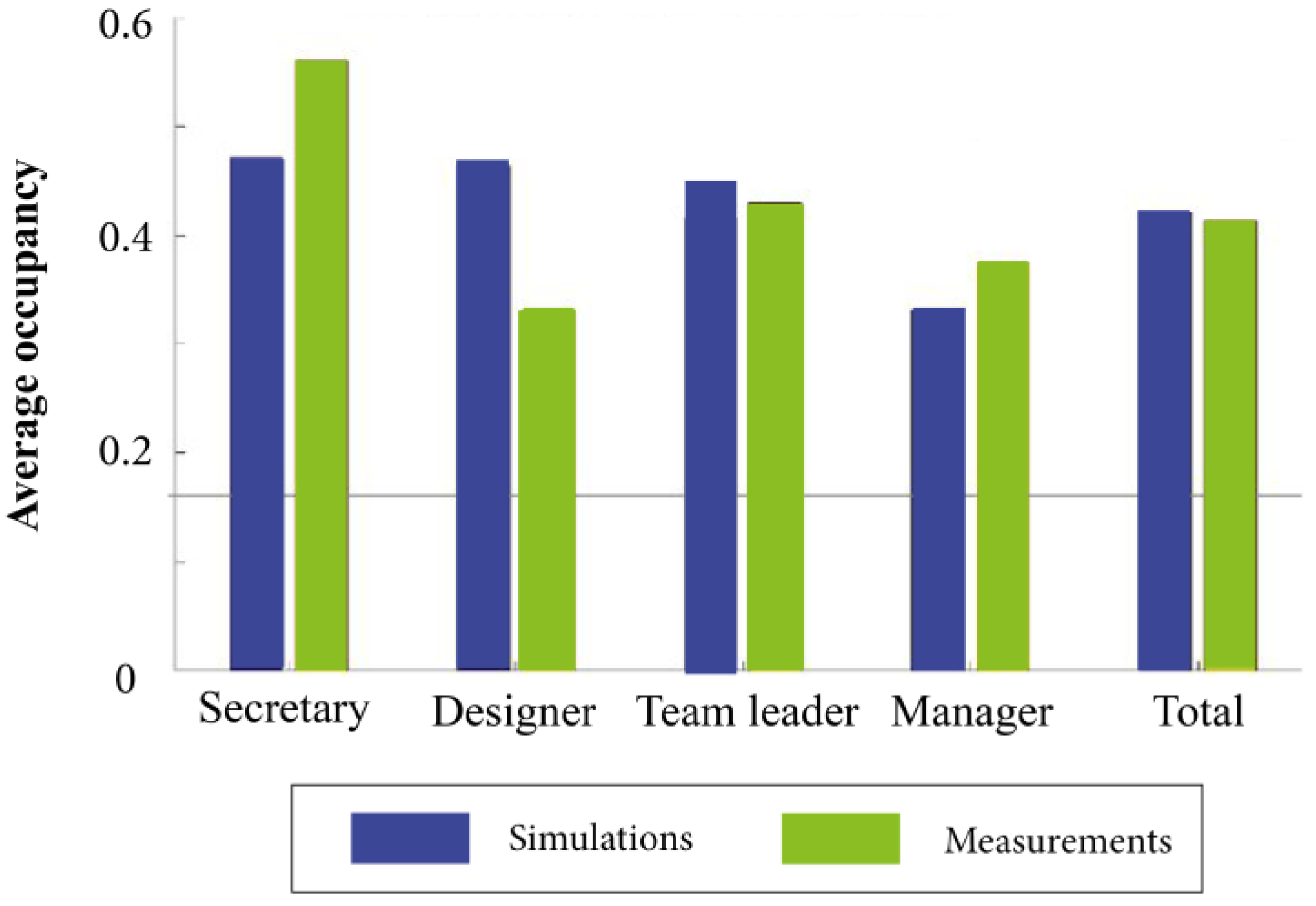
To validate the occupancy patterns generated by the model, two simulations were ran. To test the general validity of the model (1), we calculated the average room occupancy for a typical Dutch office setup of 16 occupants with varying job-function types (the mixed distribution from Table 2) and a loose policy (see Table 3). These results were compared to values found in the literature, specifically, those by ASHRAE 90.1-2004 [25] and in the studies of Bouffaron [16] and Duarte et al. [15]. To test the validity of the job-function type (2), simulations were performed for an office case with actual occupancy data on four job-function types: Secretary, Designer, Team Leader, and Manager [30]; this data was collected in a Dutch office environment through an observation study. To be able to compare the simulation results to this data, the model was set according to the measured and documented results regarding (a) function distribution; (b) daily start time; and (c) the number of working hours. Full-day absences were excluded because the measurement period was too short to confidently express annual values for these occurrences.
Relationship between Occupancy Spread, Lighting Energy Use, and Average Occupancy
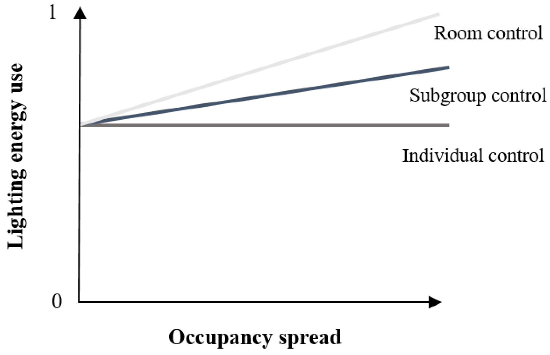
To validate the relationship between the occupancy spread and the lighting energy use, we plotted it; we expected it to be shaped as depicted in Figure 3. We reasoned that the trend lines of the individual, subgroup, and room control would meet where the occupancy spread was zero. In addition, the lighting energy use of individual control should be independent of the spread in occupancy patterns, as this strategy tailors the lighting precisely to individual occupancy patterns. Therefore, we expected its trend line to be horizontal. For both subgroup and room control, energy use should increase when the occupancy spread increases.
Additionally, for each of the points in these relationships, we calculated the average occupancy values to test our calculation method for the relative spread from Section 2.1.4: the average room occupancy should be high with a low spread and low with a high spread.
Convergence Analysis
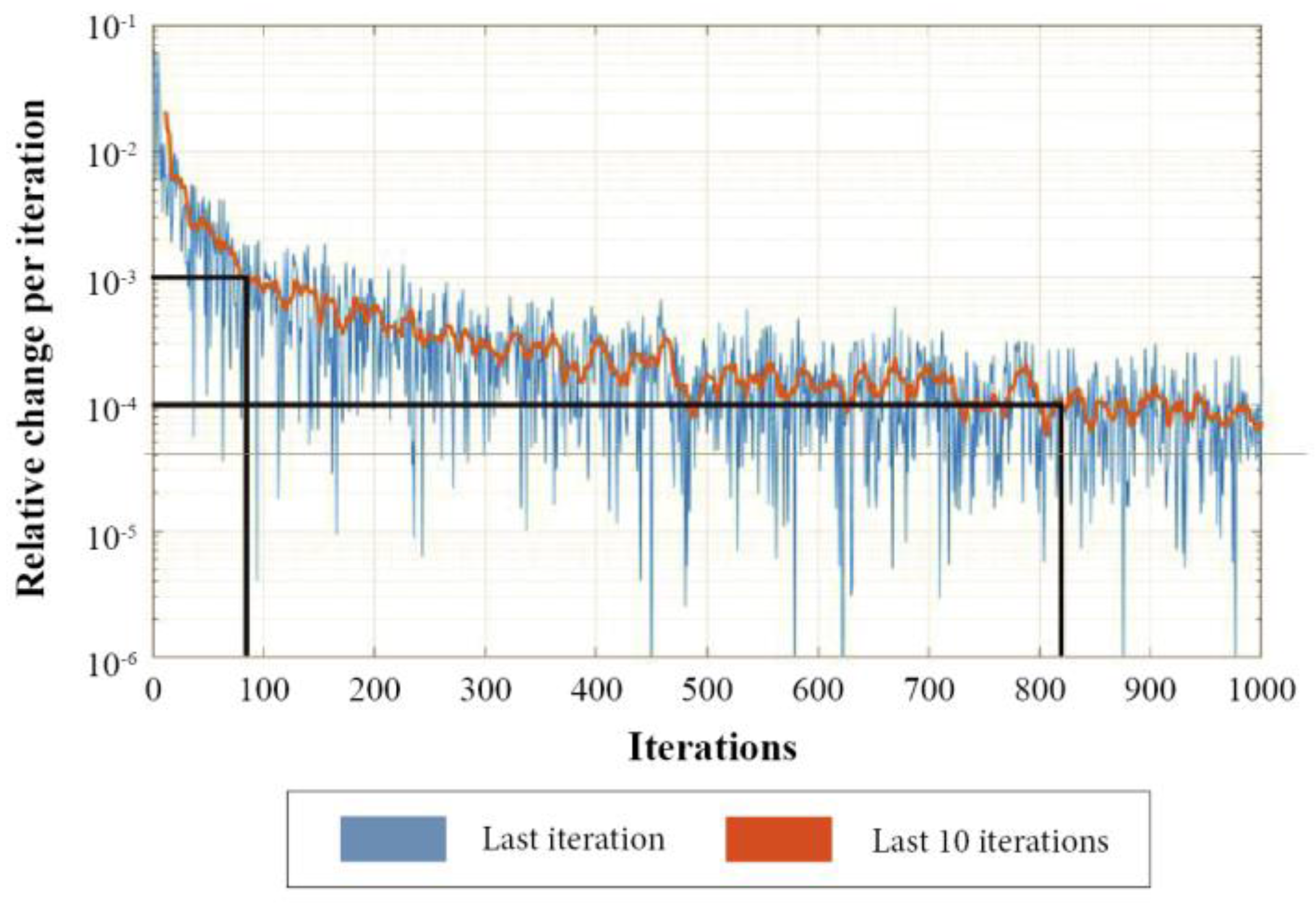
Lastly, in stochastic modeling, it is necessary to run a large number of simulations to converge toward a reliable average outcome, as each iteration can provide different results. Therefore, a convergence analysis was performed, meaning that we determined how many iterations were required to have an average relative change in of roughly 10−4; this is the value recommended by the literature for a converged solution in stochastic modeling [31].
2.2.2. Assessing the Influence of Occupancy Pattern Variance
As explained above, all simulations were performed for a fictive office consisting of 16 desks, each equipped with their own occupancy sensor and LED luminaire.
Office Policies
Two different office policies were tested. With a strict policy (1), office workers had less flexibility regarding both their start and lunch-break times, compared to a loose office policy (2). This meant that with a strict policy, individual occupancy patterns might varied less than with a loose policy. Table 4 shows the input parameters used for the two policies; though they varied in work start times and lunch start times, all other parameters were set similarly. Their values were chosen to represent a typical Dutch office; they were all based on government data (SCP, 2013).
Function Type Distributions
To determine the influence of function type distribution, five different mixtures of 16 employees having eight different function types were investigated. The differences between the occupancy patterns of the function types can be found in Table 2 in Section 2.1.2. The mixtures—or function type distributions—ranged across the extremes: from highly mixed, consisting of eight different function types (see the column ‘Mixed’ in Table 3), to completely uniform, with all 16 occupants holding the same job-function type (see the column ‘Uniform’ in Table 3). The three cases within these extremes decreased in the number of different job-function types, which can be seen in the last row of Table 3.
The five function type distributions found in Table 4 were tested for the two different office policies, resulting in a total of 10 test cases. For each of these cases, the lighting energy use was calculated for individual, subgroup, and room control, as explained in Section 2.1.4. The results were plotted to be able to determine the influence of occupancy pattern variation on the energy use (Section 3.2) and to determine the relevant control zone size for the different office cases (Section 3.3).
3. Results
3.1. Validating the Model
3.1.1. Occupancy Patterns
Figure 4 shows the occupancy diversity factor for the simulated typical Dutch office case, the ASHRAE 90.1-2013 profile [25], and the profiles found in [15,16]. By “occupancy diversity factor,” we mean real-time occupancy in relation to the maximum number of possible occupancies in the space (range = 0–1). The average occupancy profile of our simulation fell within the bounds of the measured values in the literature. Its shape most closely resembled the ASHRAE profile.
For the real office case where the observations were performed, Figure 5 shows the average occupancy from these observations and from the simulations. These are provided for four job-function types and for the total office space. The results showed that our model slightly overestimated the presence of the Designers, but slightly underestimated the presence of the Team leaders, Secretaries, and Managers. However, the simulated average for the entire office space only deviated 1.6% from the measured average.
3.1.2. Relationship between Occupancy Spread, Lighting Energy Use, and Average Occupancy
For the three different control strategies, Figure 6 shows the relationships between the occupancy spread and lighting energy use. The trend line of the individual control is horizontal, meaning that the lighting energy use was independent of the relative occupancy spread with this type of control, as expected. The energy use was most sensitive to the occupancy spread with the room control; its trend line was the steepest. Thus, all the relationships met our expectations (see Figure 3). The trend lines nearly meet where the spread would be minimal, or, in other words, when all occupants always leave and enter the room together. They approximately intersect at the vertical axis; close enough to conclude that our model met this expectation, as well.
Figure 7 shows the average occupancy rates of all points from Figure 6. For all three control strategies, the values should gradually shift from red—indicating high average occupancy—to blue—indicating low average occupancy. This confirms that our calculation method of the relative spread relates correctly to the average room occupancy. With individual control, this graduation can be clearly distinguished, however, with the other two control strategies, we find that the points cluster more. This means that the relative lighting energy use was less dependent on the average room occupancy for room and subgroup control than for individual control.
3.1.3. Convergence Analysis
Figure 8 shows the relative change of the average occupancy per iteration and the moving average of the last ten iterations. After almost 1000 iterations, the relative change per iteration was only 10−4.
3.2. Assessing the Influence of Occupancy Pattern Variance
Figure 9 and Figure 10 show the average daily lighting energy use of the three control strategies for the five function type distributions for the strict and loose office policy, respectively. The energy usages differ minimally between the function type distributions for all three strategies. Between the office policies, the differences are larger; with individual control, the average energy use over the five function type distributions is 0.60 with a strict office policy and 0.67 with a loose office policy. For both subgroup and room control, the differences between the policies were, on average, 0.05.
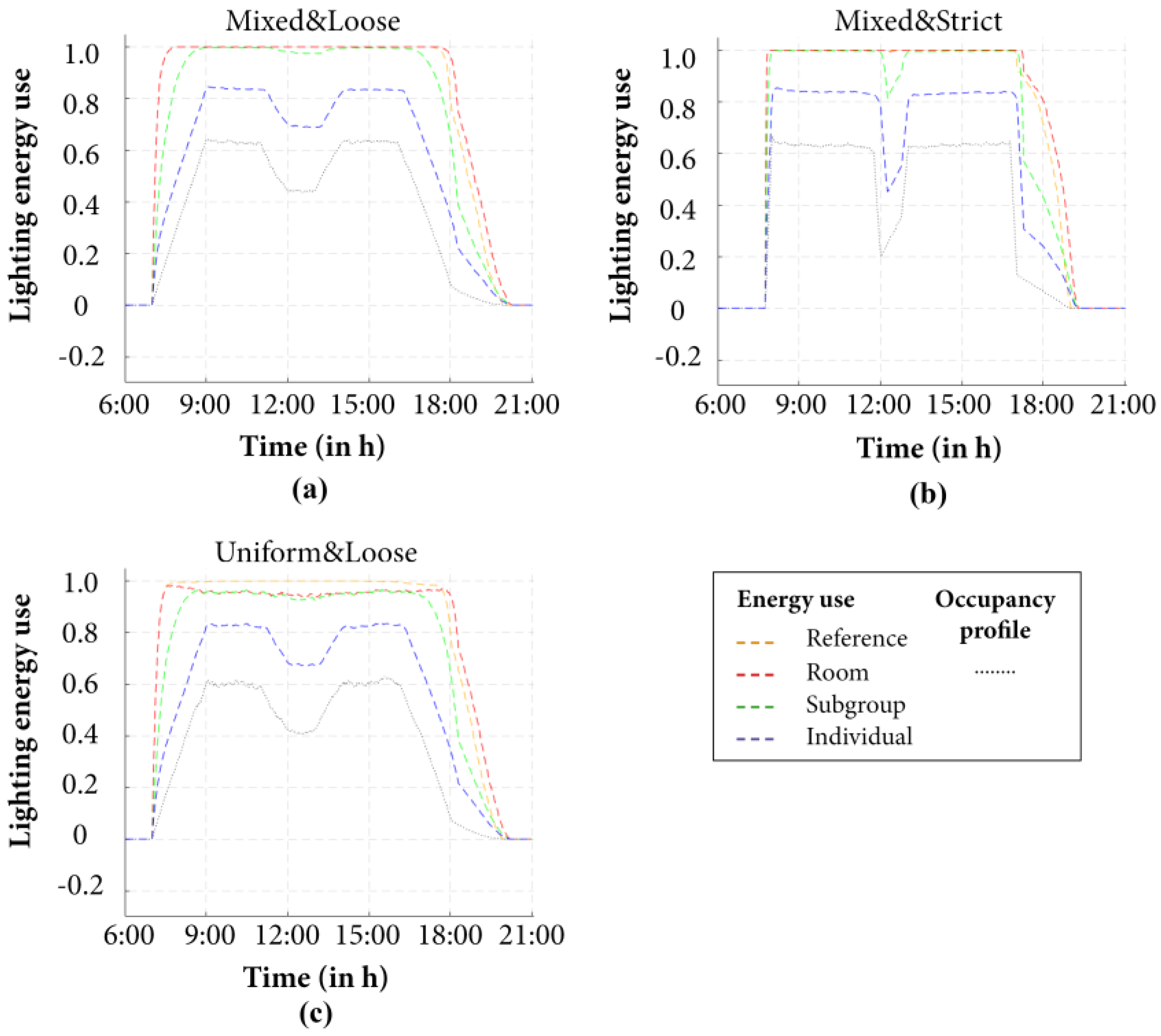
To gain a better understanding of the influence of occupancy variation, the energy use of the three control strategies were plotted over the day for three example office cases: Mixed and Strict, Mixed and Loose, and Uniform and Loose, as shown in Figure 11. These cases enabled us to compare the two office policies and the two most extreme function type distributions. The figure also provides the average room occupancy. Overall, one can see that all three strategies saved the most energy at the start and end of the day, as well as during the lunch-break period when compared to the reference case. In line with the results shown in Figure 9 and Figure 10, significantly less energy was used with individual control in all three office cases compared to the other strategies. When comparing the two office policies across the Mixed cases, we see that, with the loose policy, individual lighting control saved more energy during lunch over a longer period of time than with the strict policy. This can be explained by the larger flexibility in start times and lunch duration with the loose office policy. It also causes the finding that only with the strict policy, subgroup control used less energy during lunch break than room control and the reference case. When comparing the Mixed and Uniform job-function type distributions, the Uniform case had lower energy use with the room control and the subgroup control compared to the reference case, while they were similar with the Mixed case. In the figure, one can also see that room control used more energy than the reference case at the end of the day with all three office cases.
3.3. Determining the Relevant Control Zone Size for the Office Cases
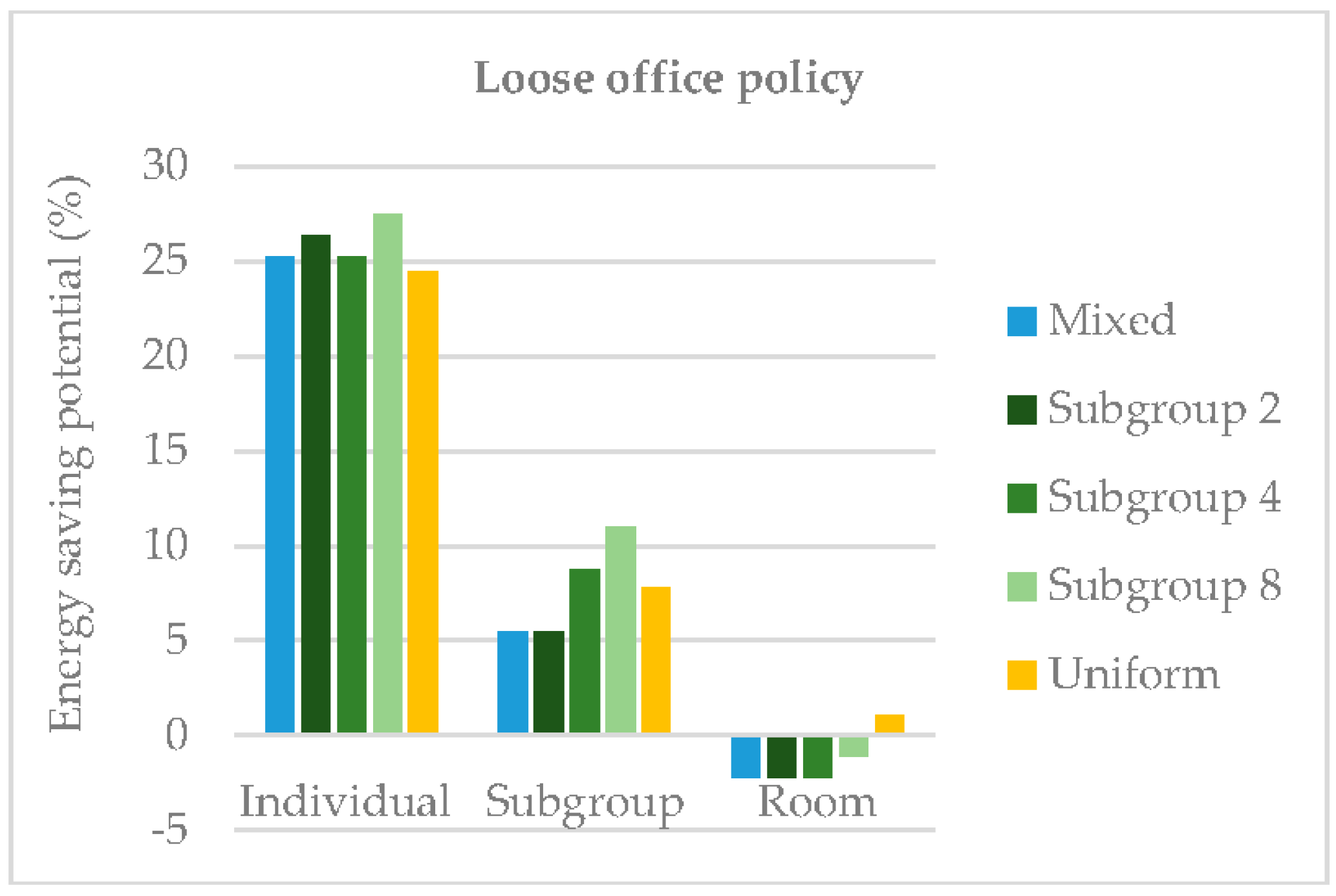
Figure 12 and Figure 13 show the energy saving potential of the three control strategies for the five function type distributions with a strict and loose office policy, respectively. They show that for all office cases, the energy savings potential of individual control is much higher than with either the subgroup control or the room control strategies: on average 30% with a strict policy and 25% with a loose policy. With room control, we found a negative relative energy savings potential with all function type distributions, except for the uniform case.
4. Discussion
4.1. Validating the Model
For this study, we developed a model to assess the energy savings potential of different control strategies for a specific office case. Most importantly, the model had to account for the stochastic nature that occurs in real life regarding users’ occupancy patterns. Overall, the different validation tests showed that the model provided realistic occupancy profiles. The average occupancy profile was a similar shape as the profiles of earlier studies, and also had similar values (Figure 4). The simulated average occupancy rates of the function types differed slightly from the measured average occupancy rates, but the overall occupancy of the space deviated only slightly—a 1.6% difference—thus demonstrating that our tool was accurate (Figure 5). In addition, the trend lines of the three control strategies for the relationship between lighting energy use and occupancy spread also met our expectations (Figure 6).
Yet, these results also suggest that more data are needed on occupancy patterns of different job-function types to make more accurate estimations. Thus, we believe more measurements should be performed—preferably in different office spaces and in different countries, to enable the use of our model internationally. More extensive data collection would also enable further fine-tuning of the model. For example, in the current model, the chance that occupants with the same job-function type were simultaneously absent due to group meetings was included, but this, of course, might also occur with occupants of different job-function types.
4.2. Assessing the Influence of Occupancy Pattern Variance
The energy savings differed only minimally between the different function type distributions (Figure 9 and Figure 10), especially with individual control. These results suggest that the job-function type distribution has almost no effect on the energy use of the different lighting control strategies. When comparing the two office policies, individual control used 7% more energy with a loose policy than with a strict policy. This can be explained by the fact that, with a loose office policy, occupants can start their day at more varying times; hence, the lighting is used a larger part of the day. In addition, when plotting the energy use over the day (Figure 11) some subtle differences came apparent during lunch break between the two office policies: subgroup control was more relevant with a strict than loose office policy. Nevertheless, as the differences were limited, our findings imply that office policy does not significantly affect the energy savings potential of the varying lighting control strategies. It suggests that the energy savings of individual lighting control found in [6,13] are likely to deviate by 7% or less when implemented in office cases with different individual occupancy patterns.
The daily profiles from Figure 11 also revealed that the highest relative energy savings potential of all three occupancy-based lighting control strategies occurs at the start and end of the day and during lunchtime. This can be explained by the average occupancy number—having the lowest value at these times. Moreover, we found that at the end of the day, lighting control at the room level used more energy than the reference case. This is in line with the negative relative energy savings potential found in Figure 12 and Figure 13, which can be explained by the time delay setting that causes the lighting to remain switched on for a while after all occupants have left the office; this does not occur with manual control.
4.3. Determining the Relevant Control Zone Size for the Office Cases
Individual control had a significantly higher energy saving potential for all office cases than the control strategies with a larger control zone when comparing their energy use to central manual control. We found the largest difference between room and individual control for the office case with the function type distribution “subgroup 8” and a strict office policy (−2% vs. 31% in Figure 13), but also the smallest difference was still 23% (for the uniform office case with a strict office policy, see Figure 13). In addition, in the worst case, individual control saved 16% more energy than subgroup control, namely with the function type distributions subgroup 4 and 8 with a loose policy. Thus, individual lighting control seems always relevant to apply in offices, independent of occupancy pattern variation. In the case of an energy savings of 16%, the installation costs might not be earned back within a five-year-period—the payback limit for commercial applications—nonetheless, its implementation would still be beneficial to the environment.
These saving amounts fall within the range of 20–60%, as identified by earlier studies for occupancy-based lighting control strategies. However, for individual lighting control, we found a relative energy savings potential of 25–30% while [6,13] found a potential of 40%. However, in these other studies, the lighting was switched off during an occupant’s absence, while in our case, we only dimmed the lighting.
4.4. Limitations
It is important to note that our model did not consider behavior where occupants might switch on the lighting for more than one control group; for example, they might trigger sensors while crossing the room to reach their desks. In addition, our model did not take into account the fact that users might forget to manually switch off the lighting in the reference scenario. However, this would result in even greater energy savings potential for automatic, occupancy-based control strategies. On the other hand, the model did assume perfect sensor accuracy, whereas, in reality, false positives or false negatives can occur. Furthermore, most parameters in our simulations, like the chance for overtime and the number of sick days, were set to the same values for all occupants, while individual differences are likely to exist in reality. However, this would argue even more in favor of individual lighting control.
4.5. Future Research Directions
This investigation focused on the influence of occupancy patterns on the energy savings potential of occupancy-based lighting control of different control zone sizes. Future research could address the effect of lighting system settings, such as dimming levels, on energy savings potential, especially because these settings seem to have a larger effect than occupancy patterns. Another important next step would be the inclusion of daylight-linked control, as this would provide more realistic energy savings numbers than can be achieved with occupancy-based lighting control. This strategy would limit the amount of time that lighting can be dimmed based on occupancy [9]. In addition, more advanced lighting needs could be incorporated. The simulation tool provides an easy and accessible method to do so, as no extensive measurements are required, and the calculations can be performed quickly over an extended period of time.
Overall, our results suggest that individual lighting control saves energy in all office cases. That said, the energy savings potential was most apparent with the loose office policy. As greater flexibility regarding work times and locations is becoming a much more common practice, researchers need to investigate this strategy further. In particular, further research is required to determine whether such practices provide comfortable work environments for office workers. As we discussed at the outset, in open-plan, European office spaces, local lighting control might not be comfortable. Additionally, while this study used the dimming levels recommended by international standards, users might have individual preferences that differ from the international standards. However, our model is able to calculate how much energy is saved when these individual preferences are met. Furthermore, the model can be used to assess other aspects of buildings’ energy use that are influenced by occupancy patterns, such as, for example, demand for controlled ventilation.
5. Conclusions
In this study, we investigated whether occupancy pattern variance within an office space influenced the energy savings potential of occupancy-based lighting control under different control zone sizes. Here, we developed a stochastic model and then undertook several validation efforts. Our work indicates that our model satisfactorily approaches real-life occupancy patterns. However, as this was just the first effort made regarding such a model, many improvements are possible, as are various extensions of the model.
Simulations were performed using the model for fictive office cases that varied in job-function type distribution and office policy to determine the possible influence of occupancy pattern variance. Our results showed that the energy savings potential at the different control zone sizes varied very minimally between the different mixtures, suggesting that the influence of occupancy pattern variance is negligible. For all office cases, individual lighting control resulted in significant relative energy savings potential of 25–30% over manual control. Especially at the start and end of the day and during lunch breaks, more energy was saved using individual lighting control compared to either subgroup or room control. These results are promising, but more research needs to done to continue investigating individual lighting control, especially with a focus on the users’ comfort.
Acknowledgments
This research was performed within the framework of the strategic joint research program on Intelligent Lighting between TU/e and Koninklijke Philips N.V. and the Impuls II SPARK program.
Author Contributions
Tom van de Voort and Christel de Bakker conceived and designed the experiments; Tom van de Voort performed the experiments; Tom van de Voort and Christel de Bakker analyzed the data; and Christel de Bakker and Alexander Rosemann wrote the paper.
Conflicts of Interest
The authors declare no conflict of interest.
References
- Commission, E. 2050 Energy Strategy. Available online: https://ec.europa.eu/energy/en/topics/energy-strategy-and-energy-union/2050-energy-strategy (accessed on 20 June 2017).
- Ryckaert, W.R.; Lootens, C.; Geldof, J.; Hanselaer, P. Criteria for energy efficient lighting in buildings. Energy Build. 2010, 42, 341–347. [Google Scholar] [CrossRef]
- Shur, M.; Zukauskas, R. Solid-state lighting: Toward superior illumination. Proc. IEEE 2005, 93, 1691–1703. [Google Scholar] [CrossRef]
- Wang, Q.; Zhang, X.; Boyer, K.L. Occupancy distribution estimation for smart light delivery with perturbation-modulated light sensing. J. Solid State Light. 2014, 1, 17. [Google Scholar] [CrossRef]
- Chung, T.M.; Burnett, J. On the Prediction of Lighting Energy Savings Achieved by Occupancy Sensors. Energy Eng. 2009, 98, 6–23. [Google Scholar] [CrossRef]
- Galasiu, A.D.; Newsham, G.R.; Suvagau, C.; Sander, D.M. Energy Saving Lighting Control Systems for Open-Plan Offices: A Field Study. LEUKOS 2013, 4, 7–29. [Google Scholar]
- Von Neida, B.; Manicria, D.; Tweed, A. An Analysis of the Energy and Cost Savings Potential of Occupancy Sensors for Commercial Lighting Systems. J. Illum. Eng. Soc. 2001, 30, 111–125. [Google Scholar] [CrossRef]
- Bellia, L.; Fragliasso, F. New parameters to evaluate the capability of a daylight-linked control system in complementing daylight. Build. Environ. 2017, 123, 223–242. [Google Scholar] [CrossRef]
- Rossi, M.; Pandharipande, A.; Caicedo, D.; Schenato, L.; Cenedese, A. Personal lighting control with occupancy and daylight adaptation. Energy Build. 2015, 105, 263–272. [Google Scholar] [CrossRef]
- Caicedo, D.; Li, S.; Pandharipande, A. Smart lighting control with workspace and ceiling sensors. Light. Res. Technol. 2017, 49, 446–460. [Google Scholar] [CrossRef]
- Pandharipande, A.; Caicedo, D. Smart indoor lighting systems with luminaire-based sensing: A review of lighting control approaches. Energy Build. 2015, 104, 369–377. [Google Scholar] [CrossRef]
- Chew, I.; Karunatilaka, D.; Tan, C.P.; Kalavally, V. Smart lighting: The way forward? Reviewing the past to shape the future. Energy Build. 2017, 149, 180–191. [Google Scholar] [CrossRef]
- Rubinstein, F.; Enscoe, A. Saving energy with highly-controlled lighting in an open-plan office. LEUKOS 2010, 7, 21–36. [Google Scholar] [CrossRef]
- Fernandes, L.L.; Lee, E.S.; DiBartolomeo, D.L.; McNeil, A. Monitored lighting energy savings from dimmable lighting controls in The New York Times Headquarters Building. Energy Build. 2014, 68, 498–514. [Google Scholar] [CrossRef]
- Duarte, C.; Van Den Wymelenberg, K.; Rieger, C. Revealing occupancy patterns in an office building through the use of occupancy sensor data. Energy Build. 2013, 67, 587–595. [Google Scholar] [CrossRef]
- Bouffaron, P. Revealing Occupancy Diversity Factors in Buildings Using Sensor Data. In Proceedings of the Behavior, Energy and Climate Change Conference, Washington, DC, USA, 7–10 December 2014. [Google Scholar]
- Chang, W.; Hong, T. Statistical analysis and modeling of occupancy patterns in open-plan offices using measured lighting-switch data. Build. Simul. 2013, 6, 23–32. [Google Scholar] [CrossRef]
- De Bakker, C.; Aries, M.; Kort, H.; Rosemann, A. Occupancy-based lighting control in open-plan office spaces: A state-of-the-art review. Build. Environ. 2017, 112, 308–321. [Google Scholar] [CrossRef]
- Creemers, P.T.J.; van Loenen, E.J.; Aarts, M.P.J.; Chraibi, S.; Lashina, T.A. Acceptable fading time of a granular controlled lighting system for co-workers in an open office. In Proceedings of the Experiencing Light 2014: International Conference on the Effects of Light on Wellbeing, Eindhoven, The Netherlands, 10–11 November 2014; p. 70. [Google Scholar]
- Roisin, B.; Bodart, M.; Deneyer, A.; D’Herdt, P. Lighting energy savings in offices using different control systems and their real consumption. Energy Build. 2008, 40, 514–523. [Google Scholar] [CrossRef]
- Jennings, J.; Colak, N.; Rubinstein, F. Occupancy and time-based lighting controls in open offices. J. Illum. Eng. Soc. 2002, 31, 86–100. [Google Scholar] [CrossRef]
- Rubinstein, F.; Bolotov, D.; Levi, M.; Powell, K.; Schwartz, P. The Advantages of Highly Controlled Lighting for Offices and Commercial Buildings. In Proceedings of the 2008 ACEEE Summer Study on Energy Efficiency in Buildings, Pacific Grove, CA, USA, 17–22 August 2008. [Google Scholar]
- Feng, X.; Yan, D.; Hong, T. Simulation of occupancy in buildings. Energy Build. 2015, 87, 348–359. [Google Scholar] [CrossRef]
- Davis, J.A.; Nutter, D.W. Occupancy diversity factors for common university building types. Energy Build. 2010, 42, 1543–1551. [Google Scholar] [CrossRef]
- ANSI/ASHRAE/IESNA. ASHRAE Standard 90.1-2016. Energy Standard for Buildings Except Low-Rise Residential Buildings; ASHRAE/IES/ANSI: Atlanta, GA, USA, 2016. [Google Scholar]
- Virote, J.; Neves-Silva, R. Stochastic models for building energy prediction based on occupant behavior assessment. Energy Build. 2012, 53, 183–193. [Google Scholar] [CrossRef]
- Ahn, K.-U.; Park, C.S. Different Occupant Modeling Approaches for Building Energy Prediction. Energy Procedia 2016, 88, 721–724. [Google Scholar] [CrossRef]
- Gaetani, I.; Hoes, P.-J.; Hensen, J.L.M. Occupant behavior in building energy simulation: Towards a fit-for-purpose modeling strategy. Energy Build. 2016, 121, 188–204. [Google Scholar] [CrossRef]
- Cowles, M.K.; Carlin, B.P. Markov Chain Monte Carlo Convergence Diagnostics: A Comparative Review. J. Am. Stat. Assoc. 1996, 91, 883–904. [Google Scholar] [CrossRef]
- European Committee for Standardization. EN 12464-1:2011 Light and Lighting—Lighting of Work Places—Part 1: Indoor Work Places; CEN: Brussels, Belgium, 2011. [Google Scholar]
- De Bakker, C.; Aries, M.; Helianthe, K.; Rosemann, A. Occupants’ behaviour: An observation study for energy saving potential on lighting. In Proceedings of the BEHAVE 2016 4th European Conference on Behaviour and Energy Efficiency, Coimbra, Portugal, 8–9 September 2016. [Google Scholar]
Figure 1.
Overview of the steps taken by the simulation model.
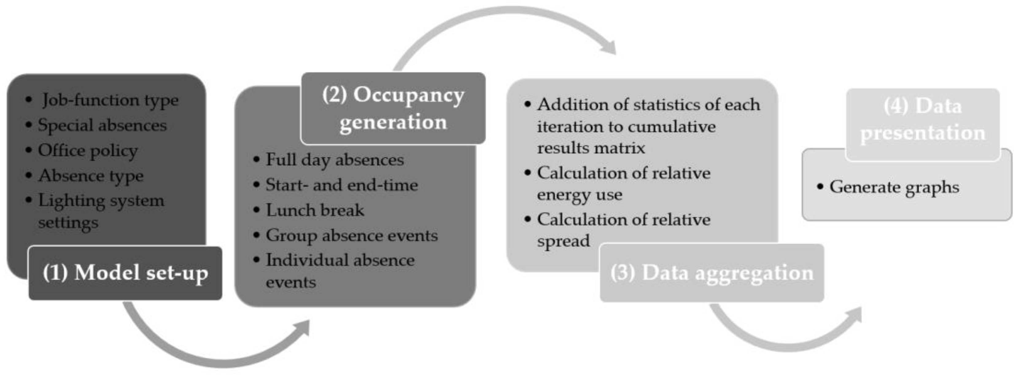
Figure 2.
Stepwise individual occupancy generation.
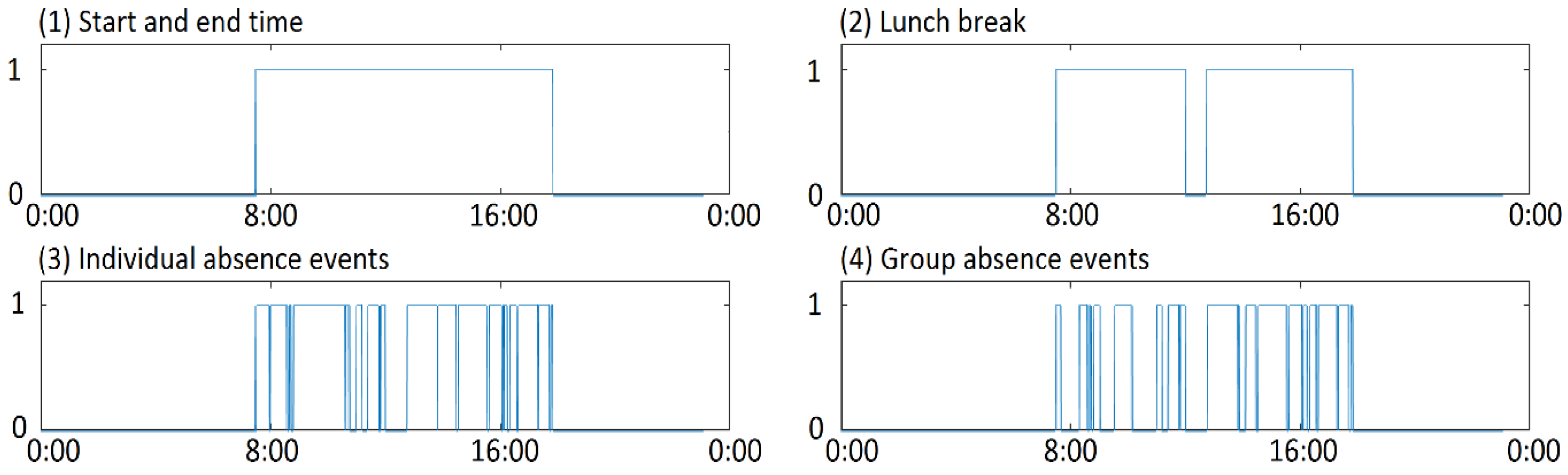
Figure 3.
The expected relationship between the relative occupancy spread and lighting energy waste for the different control strategies for an open-plan office space.
Figure 3.
The expected relationship between the relative occupancy spread and lighting energy waste for the different control strategies for an open-plan office space.

Figure 4.
Occupancy diversity factors of the validation case simulated in this study and occupancy diversity factors of earlier studies.
Figure 4.
Occupancy diversity factors of the validation case simulated in this study and occupancy diversity factors of earlier studies.
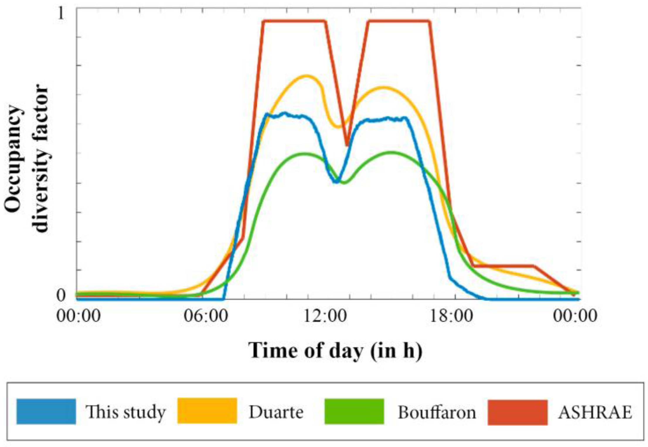
Figure 5.
Average simulated and measured occupancy for the four job-function types and the entire office space.
Figure 5.
Average simulated and measured occupancy for the four job-function types and the entire office space.

Figure 6.
Relationship between lighting energy use and occupancy spread for the three different control strategies (individual control = green, subgroup control = blue, room control = red).
Figure 6.
Relationship between lighting energy use and occupancy spread for the three different control strategies (individual control = green, subgroup control = blue, room control = red).

Figure 7.
Average occupancy versus lighting energy use and relative occupancy spread for room control (crosses), subgroup control (triangles), and individual control (circles).
Figure 7.
Average occupancy versus lighting energy use and relative occupancy spread for room control (crosses), subgroup control (triangles), and individual control (circles).
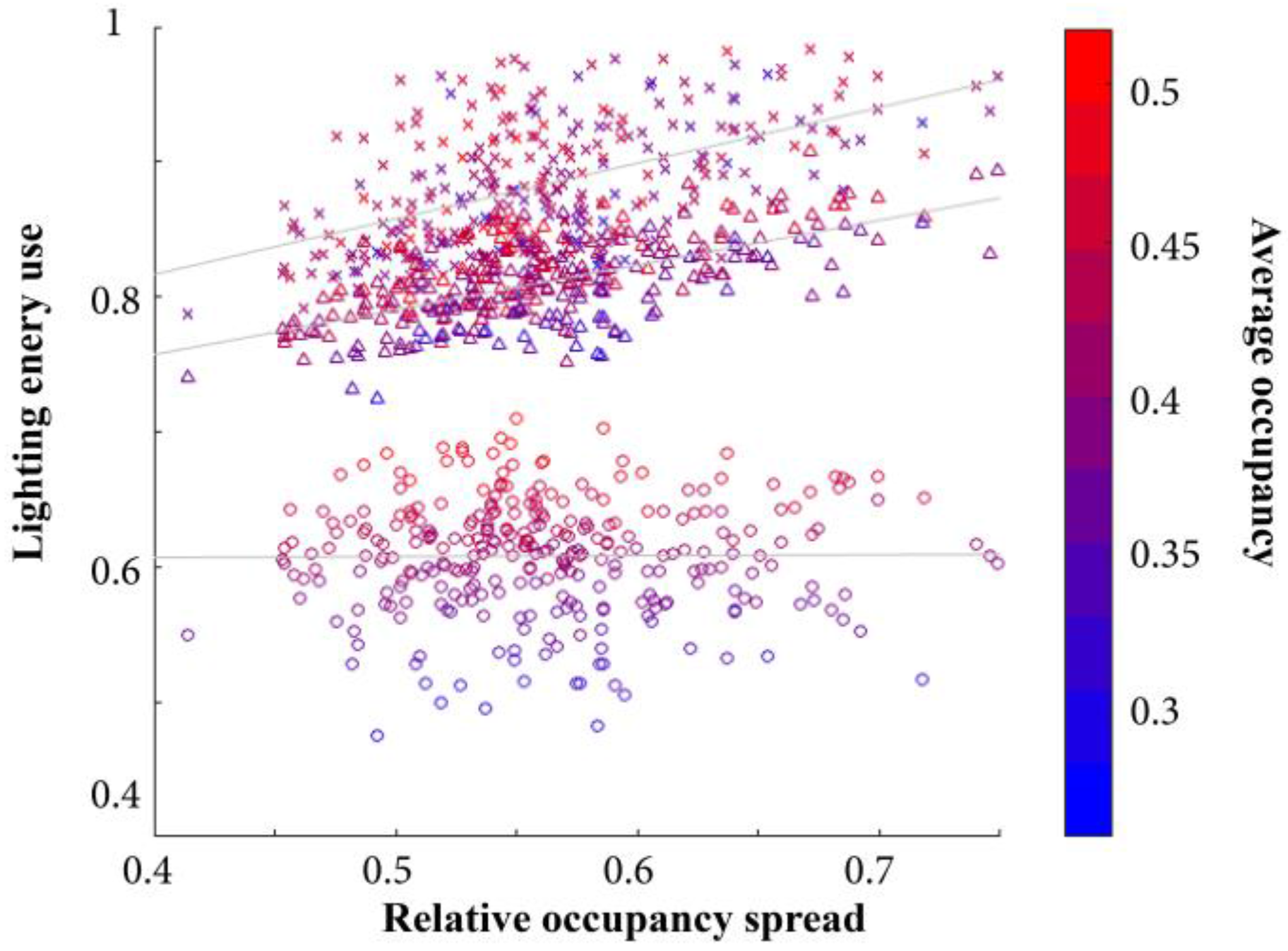
Figure 8.
Relative change in the average occupancy per iteration.

Figure 9.
Lighting energy use of the three control strategies for the five function distributions with a strict office policy.
Figure 9.
Lighting energy use of the three control strategies for the five function distributions with a strict office policy.
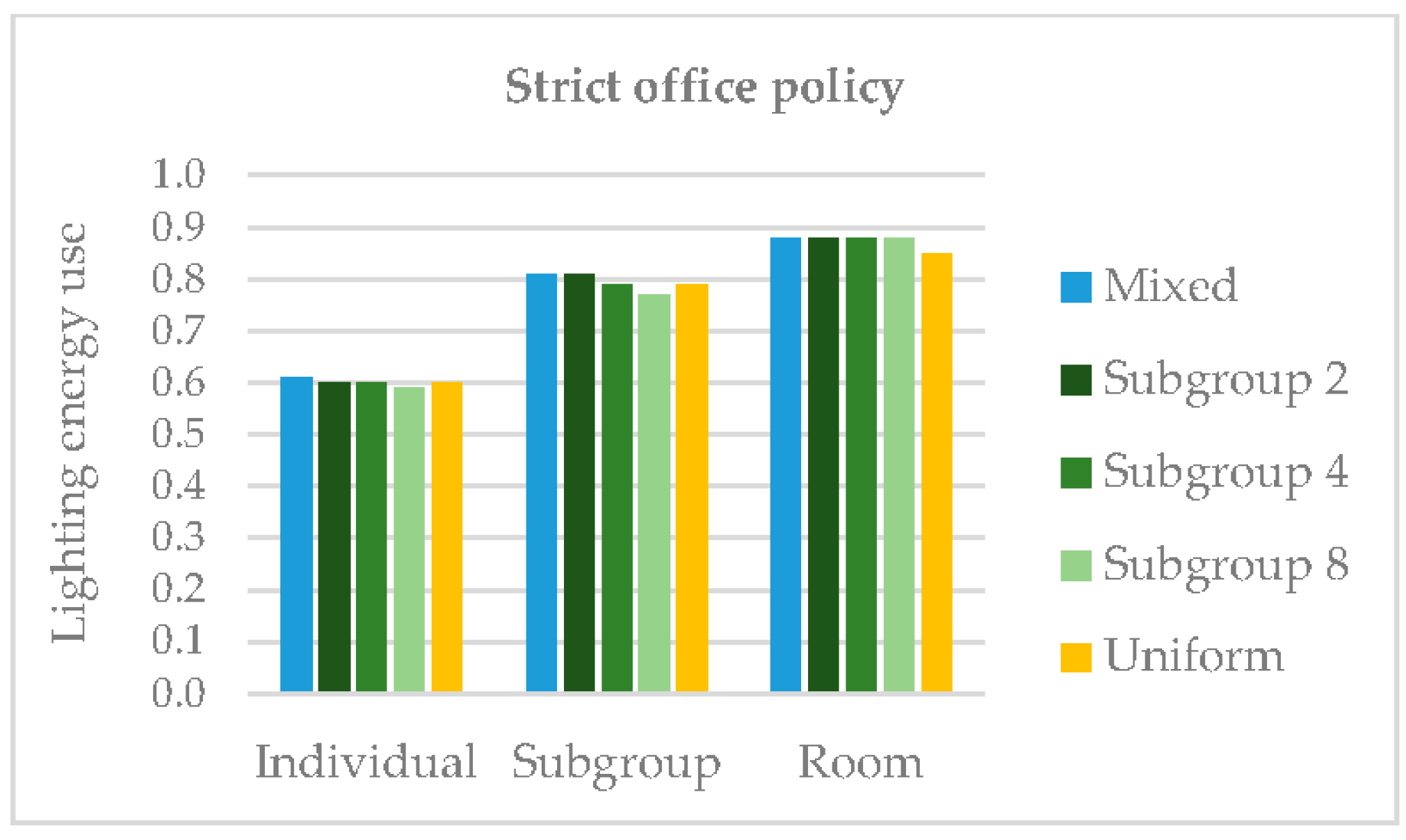
Figure 10.
Lighting energy use of the three control strategies for the five function distributions with a loose office policy.
Figure 10.
Lighting energy use of the three control strategies for the five function distributions with a loose office policy.
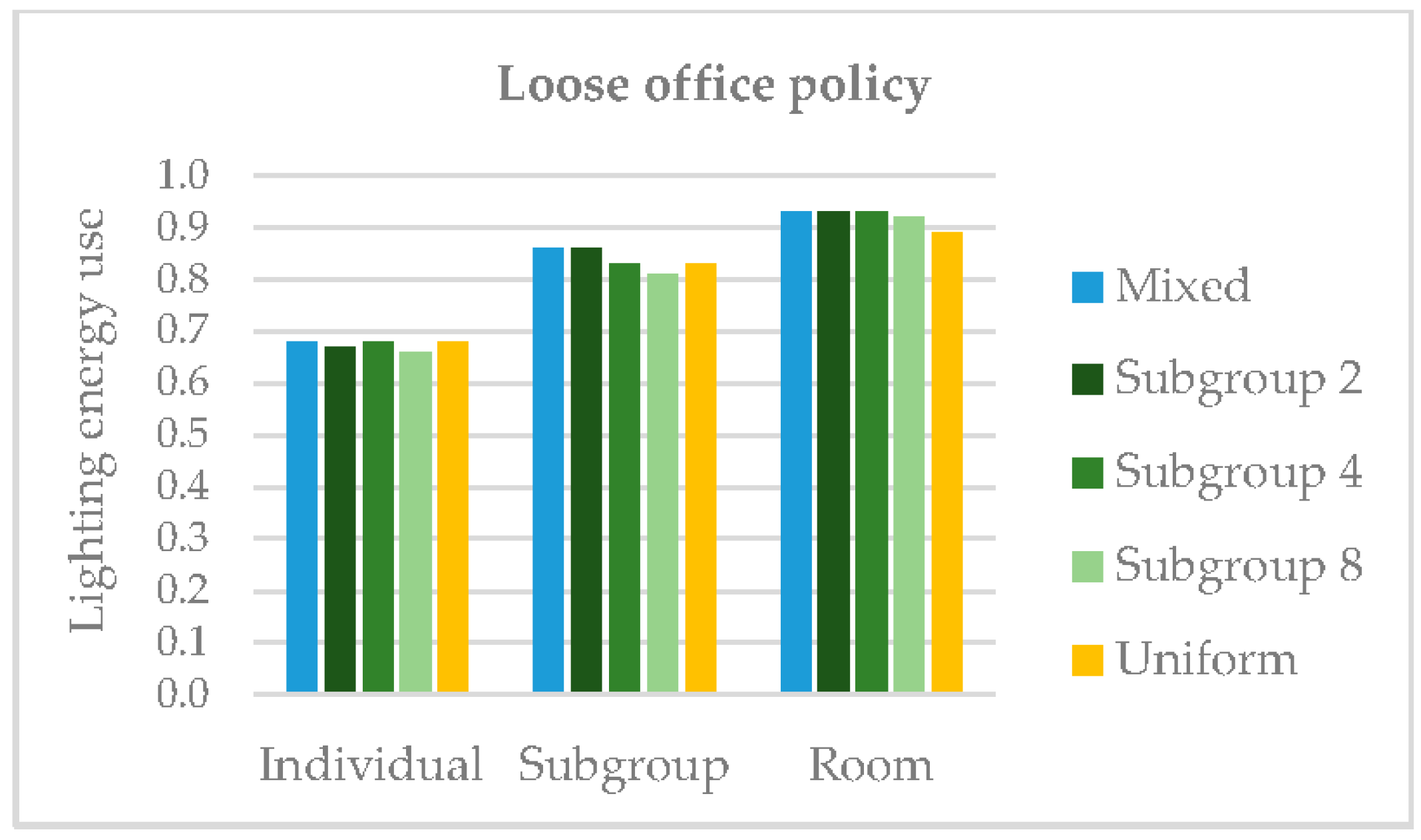
Figure 11.
Energy use over the day for the three control strategies (reference case = yellow, room control = red, subgroup control = green, individual control = purple), as well as the average occupancy profile (in grey) for three example office cases: (a) Mixed&Loose; (b) Mixed&Strict; and (c) Uniform&Loose.

Figure 12.
Energy saving potential of the three control strategies for the five function distributions with a strict office policy.
Figure 12.
Energy saving potential of the three control strategies for the five function distributions with a strict office policy.
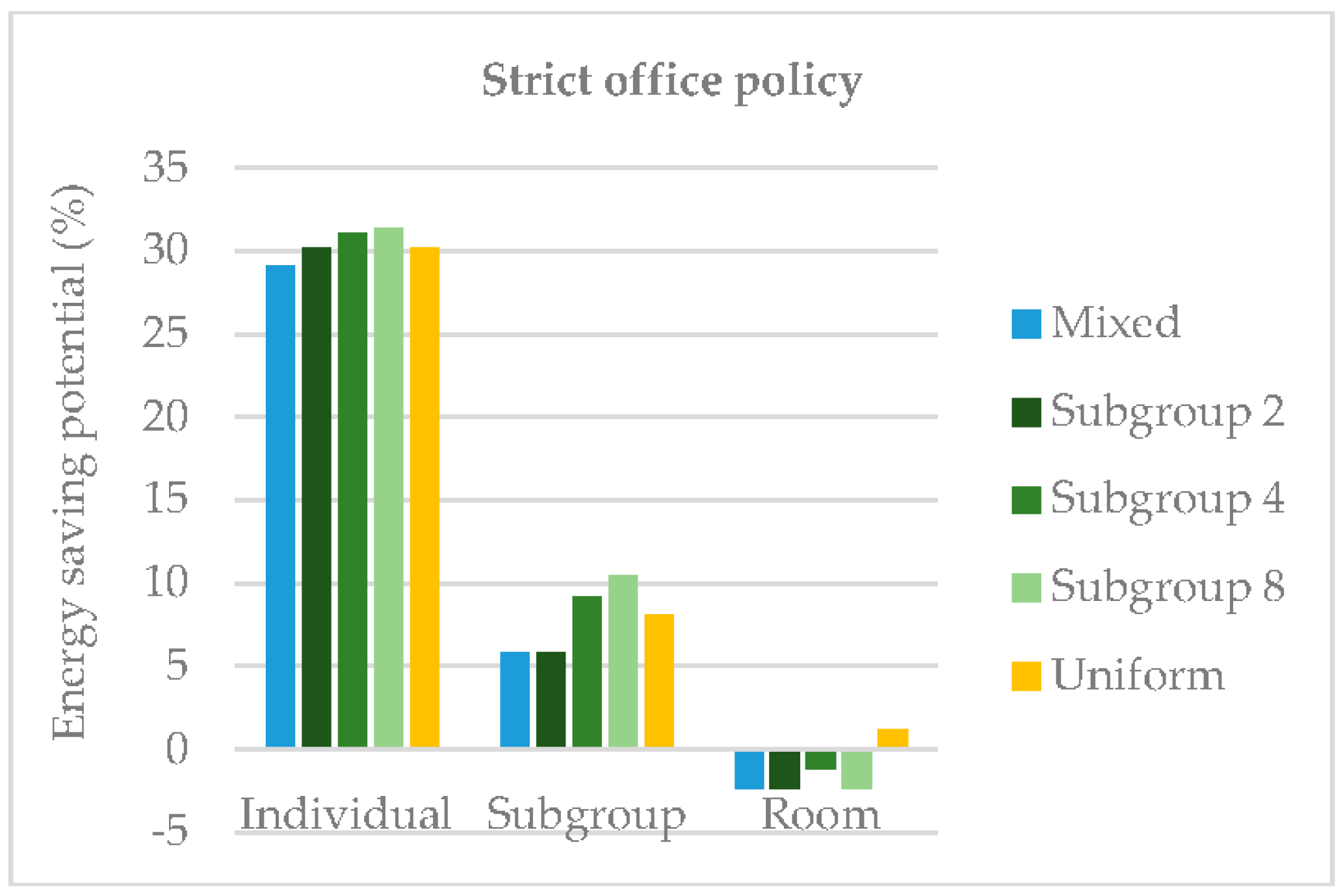
Figure 13.
Energy saving potential of the three control strategies for the five function distributions with a strict office policy.
Figure 13.
Energy saving potential of the three control strategies for the five function distributions with a strict office policy.

Table 1.
Input parameters used to define the office case when setting up the model.
| Category | Input Parameters |
|---|---|
| Job-function type | Number of absence events |
| Length of absence events | |
| Special absences | Number of holidays |
| Number of sick days | |
| FTE | |
| Office policy | Start time |
| Chance of overtime | |
| Length of overtime | |
| Number of working hours | |
| Lunch length | |
| Absence type | Ratio between individual and group absence events |
| Lighting system settings | Dimming level |
| Inactivity timer | |
| Control zone size |
Table 2.
Number of absences per duration category for the different job-function types.
| Job-Function Type | Number of Absences per Duration Category (in Minutes) | ||||||
|---|---|---|---|---|---|---|---|
| 0–5 | 5–15 | 15–30 | 30–60 | 60–90 | 90–120 | 120–240 | |
| Manager | 15 | 7 | 3 | 1.3 | 0.5 | 0.3 | 0.12 |
| Secretary | 8 | 4 | 0.5 | 0.8 | 0 | 0 | 0 |
| Designer | 25 | 4 | 1 | 0.3 | 0 | 0 | 0 |
| Drafter | 20 | 6 | 0.07 | 0.3 | 0.2 | 0 | 0 |
| Helpdesk employee | 10 | 5 | 0.2 | 0.4 | 0.1 | 0.05 | 0.05 |
| Team leader | 20 | 6 | 2 | 0.2 | 0.1 | 0.2 | 0.1 |
| Sales representative | 12 | 4 | 1 | 0.45 | 0.3 | 0.3 | 0.3 |
| Consultant | 10 | 6 | 1 | 0.2 | 0.1 | 0.4 | 0.6 |
Table 3.
Input parameters for a loose and a strict office policy.
| Category | Input Parameters | Loose Policy | Strict Policy |
|---|---|---|---|
| Office policy | Start time | 7:00 a.m.–9:00 a.m. | 7:45 a.m.–8: 00 a.m. |
| Chance of overtime | 0.2 | 0.2 | |
| Length of overtime | 1 h | 1 h | |
| Number of working hours | 8 | 8 | |
| Lunch length | 0.75 h | 0.75 h | |
| Lunch start | 3.5–4.5 h | 4 h |
Table 4.
Function type distributions for the simulation case (in bold) and the test cases.
| Function Type | Function Type Distributions | ||||
|---|---|---|---|---|---|
| Mixed | Subgroup 2 | Subgroup 4 | Subgroup 8 | Uniform | |
| Manager | 1 | 2 | 4 | 8 | 0 |
| Secretary | 1 | 2 | 4 | 8 | 0 |
| Designer | 4 | 2 | 0 | 0 | 0 |
| Drafter | 2 | 2 | 4 | 0 | 0 |
| Helpdesk employee | 2 | 2 | 0 | 0 | 0 |
| Team leader | 3 | 2 | 4 | 0 | 16 |
| Sales representative | 1 | 2 | 0 | 0 | 0 |
| Consultant | 2 | 2 | 0 | 0 | 0 |
| Number of different function types | 8 | 8 | 4 | 2 | 1 |
© 2017 by the authors. Licensee MDPI, Basel, Switzerland. This article is an open access article distributed under the terms and conditions of the Creative Commons Attribution (CC BY) license (http://creativecommons.org/licenses/by/4.0/).
Share and Cite
MDPI and ACS Style
De Bakker, C.; Van de Voort, T.; Rosemann, A. The Energy Saving Potential of Occupancy-Based Lighting Control Strategies in Open-Plan Offices: The Influence of Occupancy Patterns. Energies 2018, 11, 2. https://doi.org/10.3390/en11010002
AMA Style
De Bakker C, Van de Voort T, Rosemann A. The Energy Saving Potential of Occupancy-Based Lighting Control Strategies in Open-Plan Offices: The Influence of Occupancy Patterns. Energies. 2018; 11(1):2. https://doi.org/10.3390/en11010002
Chicago/Turabian StyleDe Bakker, Christel, Tom Van de Voort, and Alexander Rosemann. 2018. "The Energy Saving Potential of Occupancy-Based Lighting Control Strategies in Open-Plan Offices: The Influence of Occupancy Patterns" Energies 11, no. 1: 2. https://doi.org/10.3390/en11010002
Note that from the first issue of 2016, this journal uses article numbers instead of page numbers. See further details here.