A Hybrid Fault-Tolerant Strategy for Severe Sensor Failure Scenarios in Late-Stage Offshore DFIG-WT


1
State Key Laboratory of Alternate Electrical Power System with Renewable Energy Sources, North China Electric Power University, Changping District, Beijing 102206, China
2
Department of Electrical Engineering and Electronics, University of Liverpool, Liverpool L69 3GJ, UK
*
Author to whom correspondence should be addressed.
Energies 2018, 11(1), 21; https://doi.org/10.3390/en11010021
Submission received: 1 November 2017
/
Revised: 16 December 2017
/
Accepted: 20 December 2017
/
Published: 22 December 2017
(This article belongs to the Section F: Electrical Engineering)
Abstract
:As the phase current sensors and rotor speed/position sensor are prone to fail in the late stage of an offshore doubly-fed induction generator based wind turbine (DFIG-WT), this paper investigates a hybrid fault-tolerant strategy for a severe sensor failure scenario. The phase current sensors in the back-to-back (BTB) converter and the speed/position sensor are in the faulty states simultaneously. Based on the 7th-order doubly-fed induction generator (DFIG) dynamic state space model, the extended Kalman filter (EKF) algorithm is applied for rotor speed and position estimation. In addition, good robustness of this sensorless control algorithm to system uncertainties and measurement disturbances is presented. Besides, a single DC-link current sensor based phase current reconstruction scheme is utilized for deriving the phase current information according to the switching states. A duty ratio adjustment strategy is proposed to avoid missing the sampling points in a switching period, which is simple to implement. Furthermore, the additional active time of the targeted nonzero switching states is complemented so that the reference voltage vector remains in the same position as that before duty ratio adjustment. The validity of the proposed hybrid fault-tolerant sensorless control strategy is demonstrated by simulation results in Matlab/Simulink2017a by considering harsh operating environments.
1. Introduction
Doubly-fed induction generator based wind turbines (DFIG-WTs), due to their high efficiency, variable-speed constant-frequency (VSCF) operation, bidirectional power flow regulation capability, and small power electronic converter size, are widely installed, which takes over 50% of the total number of wind turbines all over the world [1,2,3,4]. Different from a fully rated wind energy conversion system (WECS), which is usually based on a permanent magnet synchronous generator (PMSG), the stator of DFIG-WT is directly connected to the grid, while the rotor is fed by a back-to-back (BTB) converter [5]. By employing this topology, the overall volume and cost of the power electronic converters are greatly reduced since only the slip power is to be regulated. However, a more complex control system is introduced. The rotor-side converter (RSC) and grid-side converter (GSC) are independently controlled, and the three-phase currents in the stator and GSC are separately measured, which means that more current sensors are equipped, adding to the hardware complexity. In addition, the rotor speed and position information should be captured by using a speed/position sensor. Therefore, the reliability of these sensors in the control system of DFIG-WT is of paramount significance to the normal operation of doubly-fed induction generator (DFIG) WECS.
It was reported in [6] that the failure rate of electrical control subsystem is around 40% for a wind turbine (WT) per year, which takes the second highest frequency of failure, and it is only lower than that of electrical system in WT. According to [7], over 14% of failures of WTs are caused by the failure of sensors. At the late stage of DFIG-WTs, the failure rate of each device swiftly increases, and it is highly possible that different categories of sensors are out of service at the same time. For example, the phase current sensors and speed/position sensor fail simultaneously, which is a severe sensor failure scenario, and the information of phase currents, rotor speed and position is lost, leading to the fact that the DFIG-WT becomes uncontrollable and has to disconnect from the grid. Especially for an offshore WT, once there is a fault that impedes the normal operation, maintenance will not be taken immediately due to high maintenance cost and low accessibility [8]. Therefore, a hybrid fault-tolerant strategy for dealing with the severe sensor failure scenario is proposed in this paper.
To obtain the rotor speed and position information, mechanical and optical sensors are usually installed in the control system of an electrical machine [9]. In addition to the increased hardware complexity and system cost, the reliability of control system is reduced as these sensors are prone to fail [10]. Therefore, different sensorless control schemes were proposed in response to the aforementioned disadvantages, which can be classified into the methods based on signal injection [11,12,13] and mathematical modeling [14,15,16,17]. Usually, the latter one is chosen for controlling induction machines (IMs) in high speed scenarios, which is also applicable for DFIG-WTs.
Apart from the deterministic sensorless control schemes, stochastic approaches can also be employed, where Kalman filter (KF) [18] is a representative of this kind of method. By taking the system uncertainties and measurement errors into account, the KF continuously minimizes the difference between the real value and the estimated one. However, for a nonlinear system, proper linearization has to be performed, which can be accomplished by applying the extended Kalman filter (EKF) algorithm [19,20]. In [21], position sensorless control of an interleaved current source inverter (CSI) fed permanent magnet synchronous motor (PMSM) drive was presented with EKF. In addition, the design and implementation of a field-programmable gate array (FPGA)-based sensorless PMSM speed control were performed with the employment of a reduced-order EKF (ROEKF) in [22], where the iteration process was significantly simplified. Besides, several studies were published to investigate modified EKF algorithms for controlling IMs. A bi input-EKF was applied in [23,24] to overcome the simultaneous estimation problem caused by the variations in stator and rotor resistances. A robust ROEKF was researched in [25] to demonstrate its superiority over an ordinary ROEKF. In [26] an interfacing multiple-model EKF was applied in the speed-sensorless vector control for IM. On top of that, the research of a speed sensorless finite-state predictive torque control (FS-PTC) based on EKF was carried out for IM sensorless control in [27]. However, there is rare literature focusing on the EKF algorithm for DFIG-WT. In [28], a suitable model was proposed for estimating the mechanical variables of DFIG. In [29], an EKF was proposed as the rotor position estimator and the observability of the DFIG was analyzed. Nevertheless, the methods proposed in these studies are only applicable when other devices are healthy, and complicated operating conditions are not considered.
In a three-phase AC/DC or DC/AC converter, two phase current sensors and a DC-link current sensor are required for obtaining phase current information and preventing the DC bus from overcurrent. To reduce the cost and increase the system reliability, the phase currents can be reconstructed according to the current information derived from the DC-link current sensor and the switching states [30]. Therefore, only one current sensor is required for providing current signals for the DFIG control system. However, immeasurable regions are created when the action time of a targeted switching state is shorter than the minimum required sampling time. A switching state phase shift method was proposed in [31] to prolong the action time for the targeted nonzero switching state so that correct current information can be obtained. While unsymmetrical pulse width modulation (PWM) waveforms are induced, which results in poorer current quality. In addition, the phase currents can be reconstructed based on current prediction strategies [32]. By combining the advantages of space vector pulse width modulation (SVPWM) technique and carrier-based PWM method, a hybrid PWM technique was proposed in [33], while the computational complexity increases. An overmodulation method was proposed in [34], which avoided voltage vector error and reduced the total harmonic distortion (THD). In [35], a tri-state PWM (TSPWM) strategy was proposed for obtaining the three-phase current information by using a single DC-link current sensor. Fixed sampling points are enabled in this method, and it is possible to enlarge the measurable area to almost the whole hexagon of SVPWM diagram, while high THD is induced in the low modulation region. Without modifying the PWM signal, a zero voltage vector sampling method (ZVVSM) [36] was proposed for phase current reconstruction to move the immeasurable regions to the edge of the SVPWM hexagon. However, the practical issues of wiring and choosing the type of current sensor are encountered.
In this paper, a hybrid fault-tolerant strategy for simultaneous failures of the phase current sensors and speed/position sensor is proposed to strengthen the reliability of late-stage offshore DFIG-WTs. A duty ratio adjustment method is proposed to improve the quality of phase current reconstruction, and the corresponding compensation strategy is put forward to avoid the variations in the amplitude and orientation of the reference voltage vector. By employing this strategy, the implementation is easy to realize, and heavy computational burden is not required. Additionally, the 7th-order dynamic model of DFIG is deeply analyzed and the robustness of EKF to system uncertainties and measurement noises is demonstrated in the sensorless control process. The accuracy of rotor speed and position estimation is investigated when wind speed step change and noises are considered. The severe senor failure scenario considered in this paper is displayed in Figure 1.
The paper is arranged in the following structure: In Section 2, the DFIG-WT modeling is carried out in terms of the wind turbine model, DFIG dynamic model and state space model. Then, the sensorless control of DFIG-WT based on the EKF algorithm is explained in Section 3. In Section 4, the phase current reconstruction strategy in BTB converter of DFIG-WT is illustrated in detail, and the proposed duty ratio adjustment scheme is presented. In Section 5, the simulation results are displayed with analysis and discussions of the proposed hybrid fault-tolerant sensorless control scheme. In Section 6, the discussion and future work in an experimental rig are explained. Finally, the conclusion is derived in Section 7.
2. DFIG-WT Modeling
2.1. Wind Turbine Model
According to wind turbine aerodynamics, the wind power input captured can be expressed as
However, only a part of the wind power captured is absorbed, and the output mechanical power of the wind turbine is
The wind power coefficient Cp is a function of the tip speed ratio λ (the ratio of the blade tip linear speed to wind speed) and pitch angle βpitch. When βpitch remains the same, there is always an optimal value of λ that maximizes the value of Cp, which is called the optimum tip speed ratio λopt. The value of Cp decreases as the pitch angle increases, and this characteristic is commonly employed in the constant speed and constant power operation regions to avoid overload of the system and extremely large output power. The expression of Cp is
where c1–c8 are the wind power coefficient parameters, with the values displayed in Table 1.
2.2. DFIG Dynamic Model
For the ease of controlling the operation and analyzing the performance of DFIG-WT, all the variables on the rotor side are referred to the stator side. The three-phase stator and rotor voltage equations are
For the purpose of independently controlling the active and reactive power of DFIG, the coordinate system transformation theory is applied to transform the three-phase variables onto the two-phase arbitrary rotating dq reference frame, and then the dynamic dq model of DFIG can be expressed by the following equations (voltage, flux, torque and kinetic equations, respectively).
2.3. DFIG State Space Model
The state variables of a DFIG include the dq stator and rotor currents isd, isq, ird, irq, rotor angular speed ωm, rotor position θm and mechanical torque Tm. Therefore, a 7th-order state space DFIG model is set up. The stator and rotor currents in the stationary two-phase αβ reference frame isα, isβ, irα, irβ are taken as measurements, and the αβ stator and rotor voltages vsα, vsβ, vrα, vrβ can are the inputs. The input u(t), measurement y(t), and state x(t), and of the DFIG system can be expressed, respectively, as
3. EKF Based Sensorless Control of DFIG
Based on the EKF algorithm, the states of a dynamic nonlinear system can be estimated with the least-square sense. In the case that the speed/position encoder fails, it is feasible to apply EKF algorithm for rotor speed and position estimation as it deals with the system nonlinearity caused by the availability of the information of ωm and θm. The optimal time-varying observer gain K(t) is obtained to minimize the estimation error, by directly taking the process and measurement noises into account.
3.1. Continuous DFIG State Space Nonlinear Model
The continuous state space model of DFIG system can be expressed as
where w(t) and v(t) are the white noises induced in the model and measurements, and they obey normal distribution. The covariance matrices of w(t) and v(t) are Q and R, respectively, which should be designed and tuned according to the model uncertainties and external disturbances in the measurements. In addition, the determination of the initial state covariance matrix P0 is also significant.
The state space DFIG dynamic model is expressed in the general form according to dx(t)/dt, which is the system transition function f(x(t), u(t)).
Based on the dq voltage and current values at the stator and rotor sides and Inverse Park Transformation, the measurement matrix of the system can be derived as
3.2. Discretization of the DFIG State Space Nonlinear Model
A discrete model of DFIG can be obtained for digital control purpose by applying Euler approximation [37]. When the sampling time Ts is relatively small, the changing rate of the state involved from the differential one can be expressed as
In this equation, k and (k + 1) represent the current and next time steps for the state, respectively. Specifically, the electrical variables in the next state are
A more accurate approximation is available for the mechanical rotor speed/position by Taylor series expansion [38,39], and the discrete expressions for ωm and θm are illustrated as
The mechanical torque can be assumed to be a constant during a short period of time, since the turbine inertia is a large value.
Therefore, the discrete process function of the state can be derived as shown below.
The discrete measurement matrix has almost the same format as the continuous one, except that the variables used are discretized ones.
Based on Equations (13), (14), (22) and (23), the system and measurement processes for the discrete DFIG state space model are obtained as
3.3. EKF Algorithm
Two steps are involved in the EKF algorithm: the prediction and update steps. The estimation of the state space variables at the next time step is obtained in the prediction step, while the error between the real and estimated values are minimized in the update step. The EKF algorithm is summarized in Table 2.
4. Phase Current Reconstruction
4.1. Single Sensor Based Phase Current Reconstruction Strategy
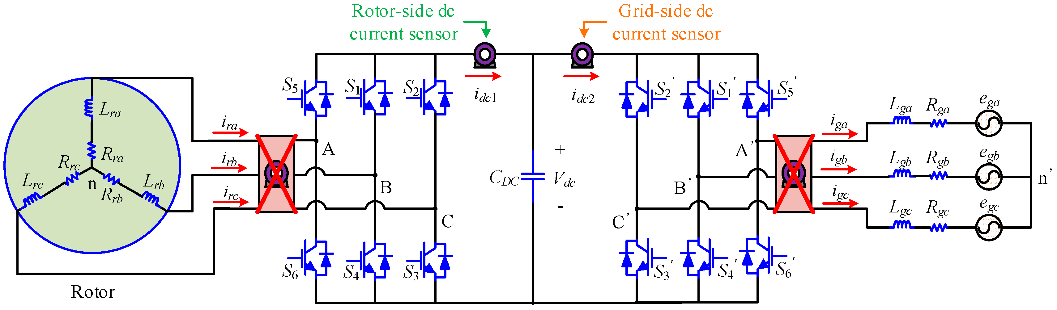
At the late stage of service time for DFIG-WT, phase current sensor failure at the RSC or GSC side is easy to happen. Traditionally, two phase current sensors are required at the AC side of RSC/GSC, and a DC-link current sensor is installed to prevent overcurrent. Considering the severe sensor failure case that the phase current sensors at both the RSC and GSC sides are not available, only one DC-link current sensor is applied for each converter to obtain the phase current information, as shown in Figure 3.
Since the values of idc1 and idc2 are, respectively, related to the switching states of the switches S1–S6 in RSC and those of S1’–S6’ in GSC, along with the three-phase currents flowing through these switches, it is possible to deduce the expressions for the phase currents by using the switching states and the DC current values. The switching state of each bridge arm is defined as Sp (p = a, b, c for RSC or a’, b’, c’ for GSC), which is equal to 0 (upper switch off and lower switch on) or 1 (upper switch on and lower switch off).
In total, there are eight switching states for each converter, which are represented by the voltage space vectors Vabc and Va’b’c’ for RSC and GSC. The connection of either the three-phase load or the three-phase voltage source is in the star format without additional line. Therefore, the following conditions are satisfied.
Take the supersynchronous operation mode of DFIG as an example, where the current flows are depicted in Figure 3, the relationships among the currents at the DC and AC sides for RSC and GSC are derived, as shown in Table 3.
The values of the subscripts a, b, c, a’, b’ and c’ can be either 0 or 1, and the relationship between the dc-link currents and the AC currents can be summarized as
It can be seen in Table 3 and Equations (28) and (29) that the phase current information in one phase can be captured when non-zero switching states are presented, and the currents in other phases can be calculated based on the phase current information obtained in different switching states in a switching period Tsw, and high precision in phase current reconstruction can be ensured when Tsw is small enough. In the space vector modulation (SVM) technique for three-phase converters, there are two zero vectors V000 and V111 that are used to complement the remaining time in a switching period, and it is impossible to get the phase current information from these switching states.
4.2. Current Sampling in Different Sectors
The space vector distribution for a six-switch three-phase converter is shown in Figure 4.
It can be seen in Figure 4 that a regular hexagon is formed in the αβ plane by the six nonzero voltage vectors, and the plane is divided into six sectors. The case when the output voltage vector VO is located in Sector I is illustrated in this figure, and the vector components of VO on the two-phase stationary reference frame are VOα and VOβ, respectively.
According to the algorithm presented in Figure 5, the value of sector indicator N can be calculated, and then the location of the output voltage vector VO will be determined.
The corresponding relationship between the value of N and the position of VO is illustrated in Table 4.
Based on the algorithm in Figure 5 and the relationship given in Table 4, the sector identification process can be accomplished. In each sector, the two basic voltage vectors at the boundaries are used as the active nonzero voltage vectors for synthesizing the output voltage vector. Along with the participation of the two zero voltage vectors in a switching period, seven segment based symmetrical PWM switching patterns are derived for the three switching states Sa, Sb and Sc. By employing this method, the number of switching times is minimized and the current distortions are mitigated to the greatest degree. In a switching period Tsw, the switching time allocated to each active vector is Tabc (the values of a, b and c can be 0 or 1), and the ratio of Tabc to Tsw is defined as the duty ratio, which is a value between 0 and 1 to indicate the proportion of switching period allocated for a specific voltage vector Vabc.
The synthesis principle of the output voltage vector in different sectors can be described as
The expressions for the duty ratios of the switches in three bridge arms are obtained as
The DC-link currents idc1 and idc2 are sampled in the nonzero switching states. Since the current relationships in RSC and GSC are identical, the general expressions for the DC and AC three-phase currents are idc and ia, ib, ic, respectively, for simplicity. The switching patterns and the corresponding values of idc in different switching states are illustrated in Figure 6.
In each switching period Tsw, four samples are derived for idc. For example, the values of ia, −ic, −ic, ia are obtained one by one for calculation of the three-phase current values. The sampling points are located at the end of the active switching state periods to avoid the fluctuations in the current signals at the beginning of new switching states.
4.3. Current Reconstruction Dead Zones
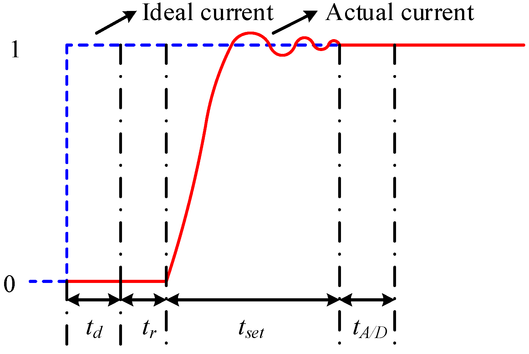
Although the fault tolerance is enhanced and the cost is reduced by applying only one DC-link current sensor for deriving the phase current information, the ever existing problem by utilizing this method is that reliable DC-link current information is not always available since it takes time for current sampling. If the time period for a nonzero switching state in a switching period is smaller than the minimum required time Tmin, then it is impossible to get the required current information at this point. The minimum required time Tmin includes the rise time tr, dead zone time td, settling time tset and A/D conversion time tA/D, and its expression is
Therefore, during the process of activating a power switch, it is impossible for the actual current value to follow the ideal one, and the comparison between the ideal and actual current values in the turning on process is illustrated in Figure 7.
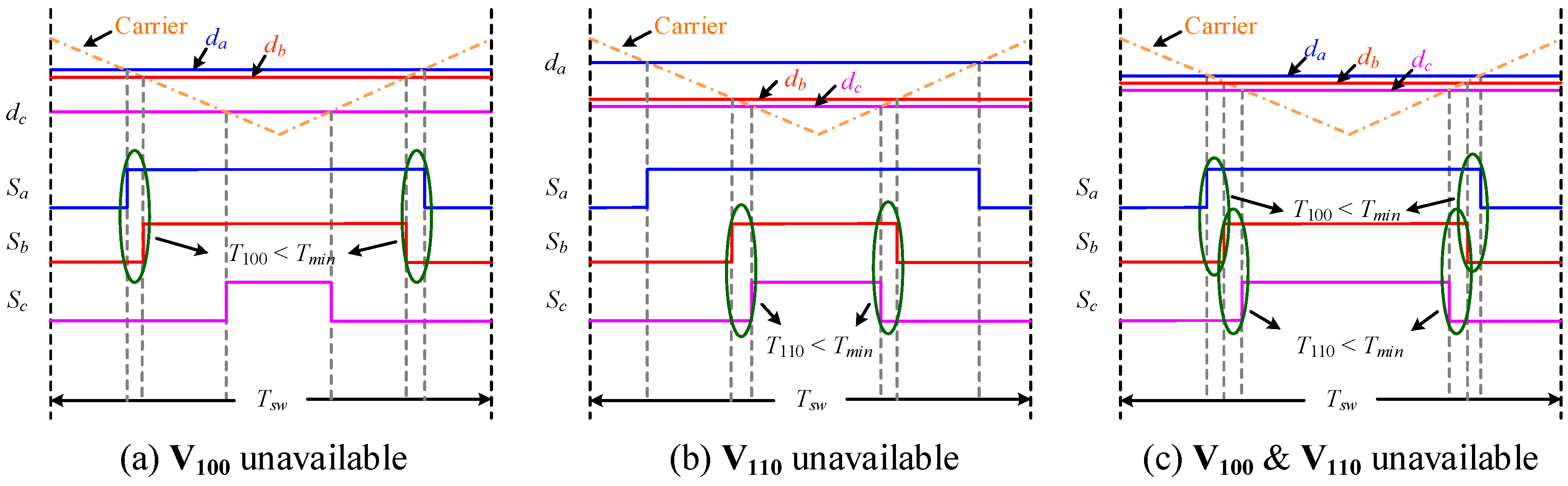
When the lasting time for one nonzero switching state is shorter than Tmin, two sampling points are missing in a switching period, and the reconstructed phase currents are greatly distorted as the DC-link current information for the specific nonzero switching state is based on that derived in previous switching periods. Under this circumstance, a phase current reconstruction dead zone is formed at the boundary of two sectors. Even worse, in the case that both the nonzero switching states are on for no longer than Tmin, more severe reconstructed phase current distortions are presented. In this case, it indicates that low modulation index is used and the output voltage vector is in the low modulation region. Take the case when VO locates in Sector I as an example, the PWM switching patterns for three situations with current sampling failures are displayed in Figure 8.
In Figure 8a, the action time of V100 is smaller than Tmin, and in this case the output voltage vector VO locates in the unmeasurable area at the boundary of Sector I and Sector II. When the situation described in Figure 8b occurs, VO locates in the sector boundary area between Sector I and Sector VI. In addition, when the output voltage vector is in the low modulation region, the corresponding PWM switching patterns are shown in Figure 8c, where no sampling points are presented in a switching period. The current reconstruction dead zones including the sector boundary region and low modulation region in the space vector diagram are depicted in Figure 9, with the cases in Figure 8 illustrated.
In Figure 9, it can be seen that, only when the output voltage vector is neither in the low modulation region nor sector boundary region, the correct phase current information can be captured. In this case, the quality of the reconstructed three-phase currents is poor and not possible for closed-loop control of DFIG. Therefore, it is necessary to solve this problem by providing a feasible compensation scheme.
4.4. Proposed Duty Ratio Adjustment Scheme
To prolong the action time of the nonzero voltage vectors to make sure it exceeds or equals Tmin, a duty ratio adjustment scheme is proposed to shift the PWM switching patterns to the desired positions. Take the case of Figure 8a as an example, as the action time of V100 is not enough, an additional time period T100_add is added to T100 to extend it to the minimum required value. The switch-on time of V100 is related to the distance between da and db, and the relationship between the pulse width and duty ratio difference is displayed in Figure 10.
Since the pulse width pattern is symmetrically placed in a switching period, the active time T100 is evenly distributed into two parts in each half switching period, and the following condition must be satisfied in order to reliably measure the desired current values.
If Equation (34) is not satisfied, then T100_add/2 should be added to T100/2 in each half switching period. It is realized by adjusting the value of da or db, and the duty ratio to be complemented is
Similarly, the compensating duty ratio components for other duty ratios in different sectors are calculated in the same way as that in Equation (35). With the purpose of keeping the pulse width switching patterns symmetrical, only the largest and smallest duty ratios in a switching periods are to be adjusted, i.e., adding the complementary duty ratio component between the largest and medium duty ratios to the largest one, and subtracting that between the smallest and medium duty ratios from the smallest one. The details of duty ratio adjustment in each sector are illustrated in Table 5.
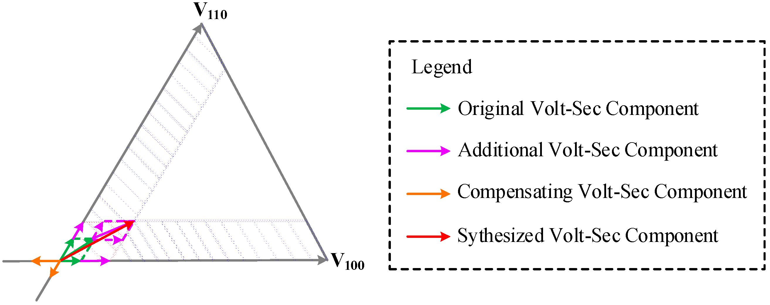
Although the missing switching states are recovered by adjusting the values of corresponding duty ratios, the side effects that are generated by using this method is that the output voltage vector deviates from its original position, along with the variation in its magnitude. Under such a circumstance, the voltage vector locus is not smooth enough for maintaining sinusoidal three-phase waveforms. To mitigate the distortions that occurred in the output voltage vector, compensating switching states are required in a switching period to eliminate the redundant components caused by additional action time on the nonzero basic voltage vectors. Assume the case of Figure 8c happens, where the voltage vector locates in the low modulation region, then the basic voltage vectors V011 and V001 are employed to compensate for the surplus voltage-second integral components in the directions of V100 and V110, respectively. The space vectors after implementing the duty ratio adjustment and switching state compensation are displayed in Figure 11.
By adjusting the duty ratios, it is ensured that four sampling points are available in a switching period, which increases the accuracy of phase current reconstruction. At the end of each switching period, the compensating switching states are added so that the output vector in a switching period is kept the same as that before the implementation of the proposed strategy.
5. Simulation Results
When the severe sensor failure scenario occurs in DFIG-WT, the EKF based position sensorless algorithm and the single DC-link current sensor based phase current reconstruction method are applied simultaneously to maintain continuous operation of the system. The control block diagram of the hybrid sensorless control strategy for post-fault operation of DFIG-WT is illustrated in Figure 12, which is to be verified by simulation studies in Matlab/Simulink2017a (MathWorks, Natick, MA, USA).
The rotor speed and position are estimated by applying the EKF algorithm based on the 7th-order DFIG dynamic state space model. By measuring the DC-link currents idc1 and idc2, along with the duty ratios for the RSC and GSC, the rotor-side and grid-side three-phase AC currents are reconstructed. In the simulation process, the post-fault operation of a 1.5 MW DFIG-WT is investigated, with the initial slip set as −0.2, and the initial rotor position equals 0. The sampling time Ts is set to 5 μs. The system parameters for the 1.5 MW DFIG-WT are shown in Table 6.
In the simulation study, the wind speed change from 15 m/s to 10 m/s at t = 0.5 s is considered to verify if the estimated or reconstructed values track the real values well. The graph of wind speed is shown in Figure 13. All the simulation results shown in this section are derived by considering wind speed step change from 15 m/s to 10 m/s at t = 0.5 s.
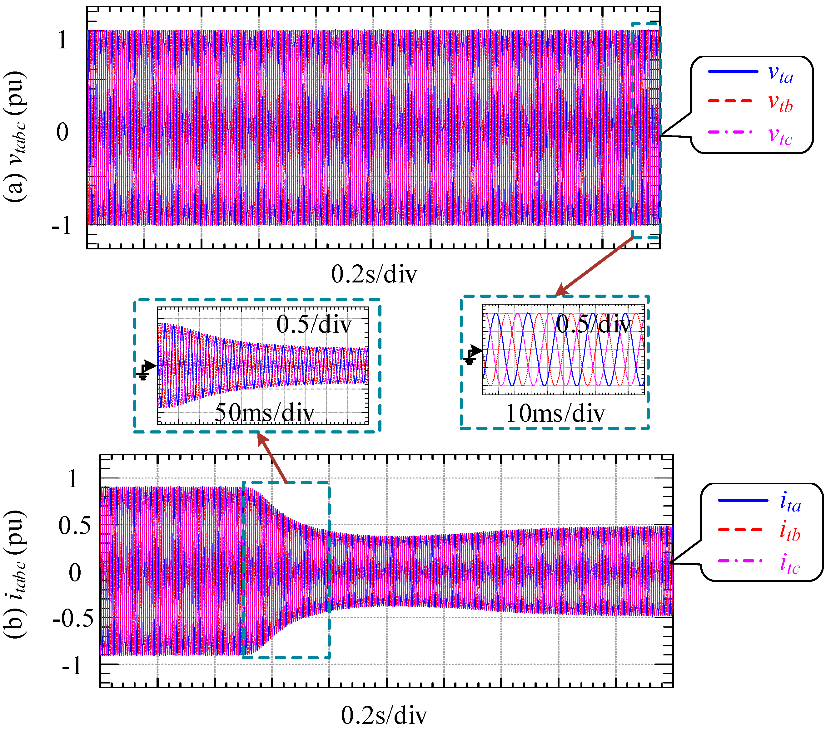
Therefore, the total output electrical power decreases at 0.5 s, and the three-phase total output voltages and currents to the AC grid are displayed in Figure 14.
In Figure 14, it can be seen that the amplitude of the phase current drops to around half the original value to maintain the balance between the input mechanical power and the output electrical power.
The three-phase currents are reconstructed to replace the functions of phase current sensors, and only a DC-link current sensor is required in this case, which saves the cost and improves the fault-tolerant ability of the control system. The real and reconstructed three-phase GSC AC currents are presented in Figure 15.
It can be seen in Figure 15 that the reconstructed current value tracks the real one accurately for each phase, which demonstrates the validity of the proposed current reconstruction strategy. With the purpose of observing the effects of the reconstructed currents on the system performance, the graphs of the total output active power (Pt), reactive power (Qt), and power factor (PF) derived when applying the measured currents and reconstructed currents, are depicted as shown in Figure 16. Moreover, when the DC current offset of 0.1 pu is taken into account in the DC-link current sensors, the corresponding graphs are also illustrated in Figure 16.
In Figure 16, it can be seen that when the measured three-phase grid-side and rotor-side currents are used, the total output active power drops from 1.5 MW to 0.8 MW after the wind speed step change, with a period of around 1 s to adjust the value to a stable one. There is also a slight increase in the reactive power output, which reaches around 0.06 MVar at 1.2 s. However, it moderately declines back to the desired value after that. In terms of the power factor, the minimum value is around 0.996 at 1.2 s, and then it returns back to unity steadily. When the reconstructed phase currents are applied as the inputs for the control system, the graphs of Pt, Qt and PF are shown as the red dashed lines in Figure 16. Although some fluctuations are observed, the errors between the values derived by using the measured and reconstructed currents are relatively small. Therefore, the DFIG-WT with serious sensor fault scenario can still work properly. Furthermore, after taking the inaccuracy of the DC-link current sensors into account, the active power output can still be tracked precisely. Even though the quality of output power is deteriorated, the average value of the power factor is high enough for acceptable operation.
In addition, the rotor speed ωm and position θm are estimated by using the EKF algorithm based on a 7th-order DFIG state space model. By directly taking the uncertainties in the stochastic process into account, the Kalman gain matrix K(k) is calculated that minimizes the error between the real and estimated values. The algorithm is performed online so that the adjustment of the components in the Kalman gain matrix is carried out according to the variations in the errors. The white noises in the model and measurement processes are determined as shown below.
To simulate the scenario that inaccurate initial estimation of the variables is presented and make the EKF estimator minimize the errors over time, the primary error covariance between any two state variables is assumed to be relatively large, and the initial state covariance matrix P0 is set as
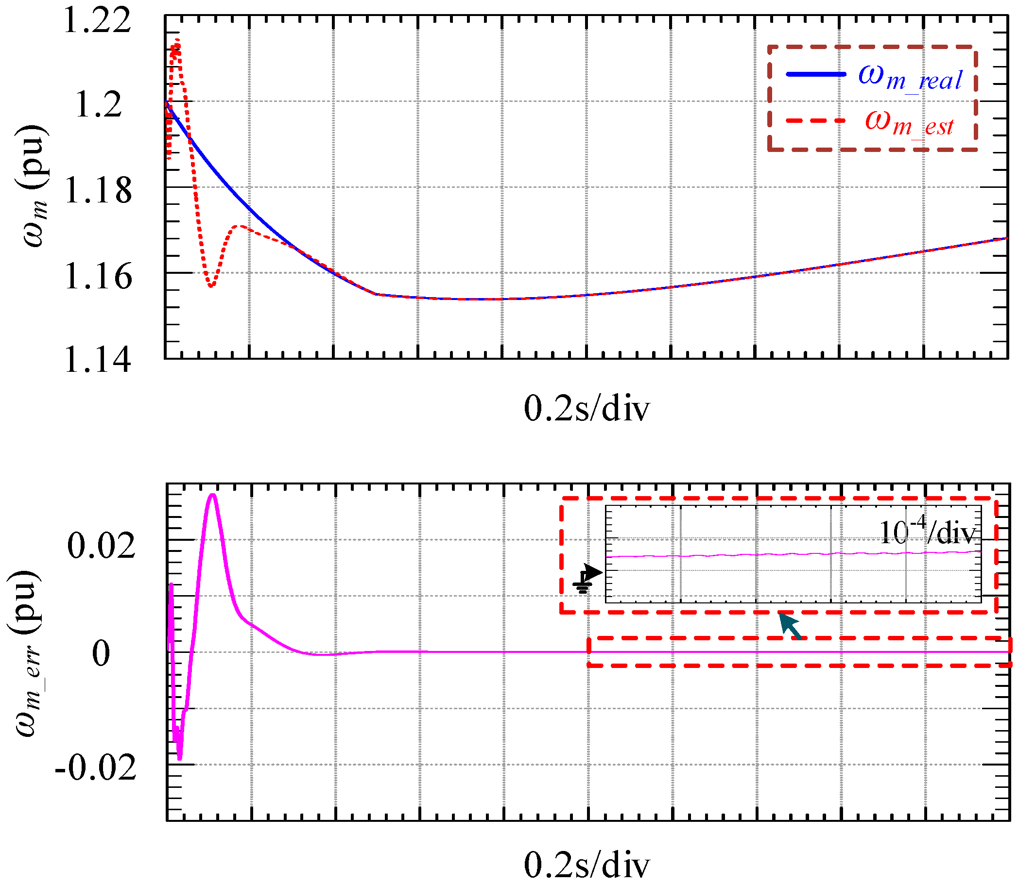
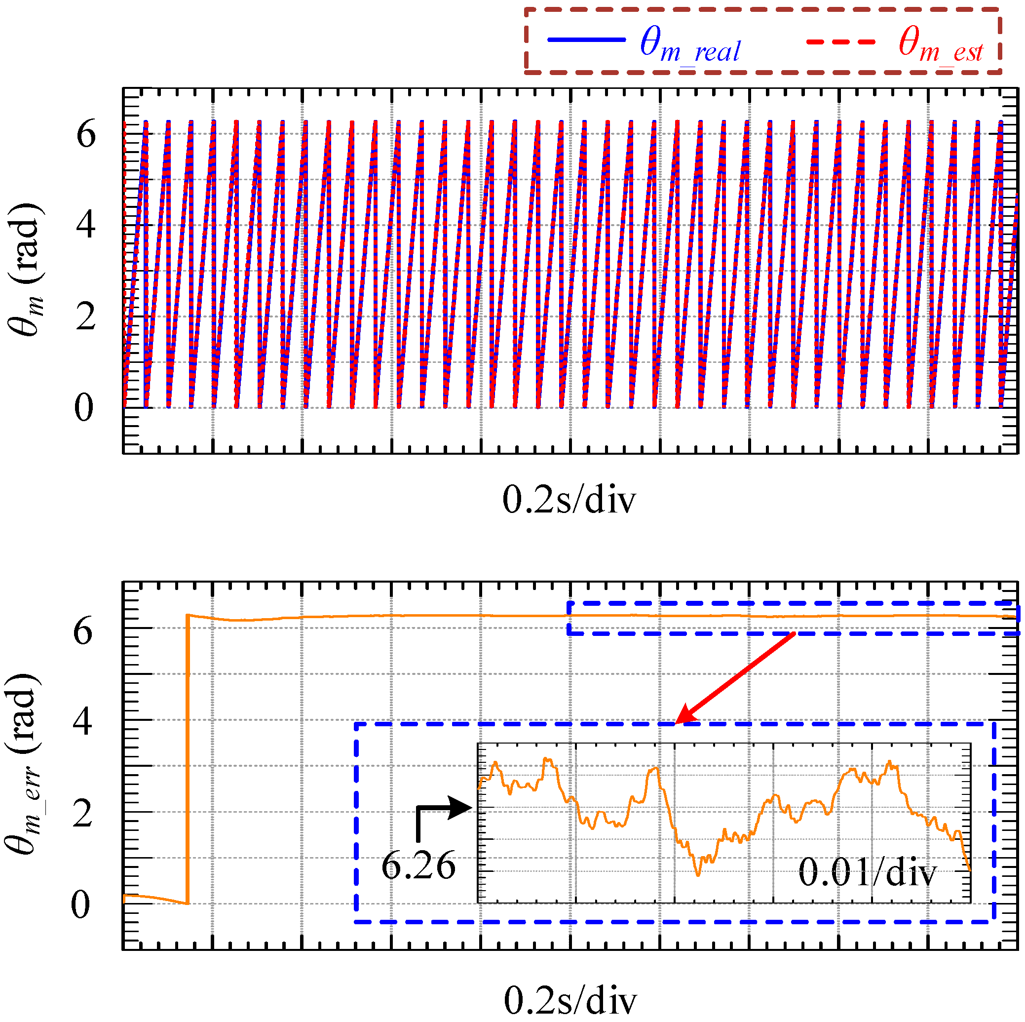
With the stator and rotor voltages as inputs, and the stator and rotor currents as measurements, the estimation of the rotor speed and position can be completed based on the recursive algorithm. The real and estimated rotor speed and position are displayed in Figure 17 and Figure 18, respectively, with the difference illustrated.
It can be seen in Figure 17 that, at the beginning, the rotor speed estimation deviates from the real value by around 0.2 pu, which is large compared to the initial rotor speed of 1.2 pu. However, in around 0.3 s, the tracking performance is good enough for the estimated rotor speed to replace the real one since the difference between them is only about 4 × 10⁻⁵ pu, regardless of the wind speed step change. In addition, the estimated rotor position is almost equal to the real one, which can be observed in Figure 18. It should be noted that the range of rotor angular position is [0, 2π]. Although the error displayed in Figure 18 is approximately 6.271 rad, it can also be expressed as (6.271 − 2π) rad, whose absolute value is only 0.0122 rad, since the rotor position is a periodic function of time. Therefore, the estimated rotor position is accurate enough for sensorless control of DFIG-WT. To demonstrate the mechanical performance of DFIG-WT, the mechanical and electromagnetic torques are displayed in Figure 19.
Since the machine operates in generator mode, the torque values are negative, indicating that the electromagnetic torque Tem functions as the load torque. It can be seen that Tem is almost equal to the mechanical one Tm in the high wind speed period. Then, during a short time period after the wind speed step change, the absolute value of Tem is larger than that of Tm, and the rotor slows down in this case. After that, the distance becomes smaller as the rotor speed tends to be approximately a steady value.
Good robustness to noises in a nonlinear dynamic system is a unique characteristic of EKF, which is also applicable for DFIG dynamic model. To further verify the validity of EFK based sensorless control algorithm for DFIG-WT, system model uncertainties and measurement disturbances are taken into account. After considering the noises in the system model and measurements, the estimations of rotor speed and position along with the differences are illustrated in Figure 20 and Figure 21, respectively.
In Figure 20 and Figure 21, although there are noises caused by system model uncertainties and measurement disturbances, the estimated rotor speed and position still track the real values well, whereas the estimation accuracy decreases. With the noises added, the EKF has to repeatedly calculate the optimal Kalman gain to minimize the error, which takes several time periods. As can be seen from Figure 20, the error between the real and estimated rotor speeds is within 4 × 10⁻³ pu, while it keeps fluctuating. In Figure 21, there is approximately a difference of 6.26 rad (0.0232 rad) between the real and estimated rotor positions, with the fluctuation of ±0.02 rad. Nevertheless, the estimation precision is still good enough as divergence does not occur in this case, and the EKF based speed/position sensorless control algorithm is demonstrated to be robust to noises.
6. Discussion and Future Work with Experiments
Although the proposed hybrid fault-tolerant strategy in a 1.5 MW DFIG-WT is verified by simulation results, experiments are going to be undertaken in the future by using a down-scaled DFIG experimental platform, including a 20 kW DFIG, a 23 kW permanent magnet synchronous motor (PMSM), back-to-back power electronic converters, and a DSpace controller. The parameters of the machines and converters should be cautiously selected according to the specific experimental conditions. In addition, tuning of PI parameters and the parameters in the initial state covariance matrix will be a time-consuming task. In the experiment, an HS01-C hall sensor (BEIJING CHUANG SI FANG ELECTRONICS LIMITED BY SHARE LTD, Beijing, China) will be chosen as the current sensor for DC-link current measurement, since it has good robustness, strong voltage isolation ability, and high reliability. The rated input and output currents of the HS01-C hall sensor are 50 A and 50 mA, respectively, with the measurement range from 0 A to 70 A, and the working temperature is between −20 °C and 75 °C.
In terms of the model behavior in the experimental rig, taking the external disturbances of uncertain grid power quality (current harmonics, grid unbalance, frequency oscillations) and the noises in analog-to-digital (A/D) process into account, deteriorated control performance will be observed. Specifically, obvious spikes will be presented in the voltage and current waveforms, and the output power quality will not be as high as that derived in the simulation results. In addition, due to the unpredictable aging process of the DC-link current sensor, the accuracy of current measurement may not be high enough, which is also detrimental to the performance of DFIG. To exclude the noises produced during the experiments, additional filters should be used.
7. Conclusions
This paper investigates a hybrid fault-tolerant strategy for riding through the severe sensor fault scenario in a late-stage offshore DFIG-WT. Under this circumstance, the phase current sensors in the BTB converter and the rotor speed/position sensor are at the faulty states simultaneously. The 7th-order DFIG dynamic state space model is analyzed, and the EKF algorithm is applied for estimating the unmeasurable rotor speed and position, and the robustness of this algorithm is verified. In addition, a single DC-link current sensor based phase current reconstruction strategy is employed for obtaining the phase current information. The current reconstruction dead zone is analyzed, and a simple duty ratio adjustment scheme is proposed to make sure the action time of each targeted switching state is not shorter than the minimum required sampling time. Moreover, compensating switching states are utilized to ensure the reference voltage vector remain the same as that before the duty ratio adjustment. According to the simulation results, the following points are summarized:
- (1)
- The total output active and reactive power is within the acceptable ranges by considering wind speed step change.
- (2)
- The three-phase AC currents from the BTB converter are properly reconstructed, and heavy computational burden is avoided.
- (3)
- The estimations of rotor speed and position are accurate enough for replacing the speed/position sensor, even if system uncertainties and measurement noises are taken into account.
- (4)
- Good mechanical characteristics of DFIG-WT are derived in the harsh operating conditions.
In the future, experiments will be performed on a 20 kW DFIG platform to further verify the proposed control strategy.
Author Contributions
Wei Li wrote the paper and did the simulations; Gengyin Li supervised the first author in writing the paper and doing simulations; Kai Ni provided technical support and revised the language; Yihua Hu checked the logic of the paper and gave some comments on revising the paper; and Xinhua Li collected some materials for the background of this study.
Conflicts of Interest
The authors declare no conflict of interest.
Nomenclature
| ρ, Sw, vw | The air density, blade area swept by wind, and wind speed |
| Pv, Po | Captured input wind power, output mechanical power of wind turbine |
| λ, βpitch | Tip speed ratio, pitch angle |
| v, e, i, φ | Instantaneous values of voltage, source voltage, current and flux |
| Vdc | DC-link voltage, upper and lower capacitor voltages |
| Em, Vm, Im | Amplitudes of the three-phase source voltages, converter voltages and currents |
| R | Resistance |
| Lm, Lls, Llr | Mutual inductance, stator leakage inductance and rotor leakage inductance |
| Lg, Ls, Lr | Inductances on the grid, stator and rotor (Ls = Lm + Lls; Lr = Lm + Llr) |
| σ | Leakage coefficient (σ = 1 − (Lm2/LsLr)) |
| CDC | DC-link capacitance |
| P, Q | Active and reactive power |
| d | Duty ratio |
| θs, θm, θslip | Synchronous, rotor and slip angular positions |
| np | Number of pole pairs |
| s | Slip |
| J | Wind turbine inertia |
| ωs, ωslip, ωm | Nominal grid angular frequency, slip angular frequency, electrical rotor angular speed |
| Tm, Tem | Mechanical torque, electromagnetic torque |
| Tabc | Action time of the switching state Vabc in a switching period |
| Ts, Tsw | Sampling time and switching time |
| Subscripts | |
| s, r, g, t | Stator, rotor, grid, total |
| a, b, c; A, B, C | Phases A, B, C; Points A, B, C |
| α, β; d, q | Direct and quadrature components referred to the stationary/synchronous reference frame |
| _rec | Reconstructed value |
| _ref | Reference value |
| Superscripts | |
| *, ^, T | Ideal value, estimated value, conjugate, and transpose |
References
- Yaramasu, V.; Wu, B.; Sen, P.C.; Kouro, S.; Narimani, M. High-power wind energy conversion systems: State-of-the-art and emerging technologies. Proc. IEEE 2015, 103, 740–788. [Google Scholar] [CrossRef]
- Hu, J.; Yuan, H.; Yuan, X. Modeling of DFIG-Based WTs for Small-Signal Stability Analysis in DVC Timescale in Power Electronized Power Systems. IEEE Trans. Energy Convers. 2017, 32, 1151–1165. [Google Scholar] [CrossRef]
- Rezaei, E.; Ebrahimi, M.; Tabesh, A. Control of DFIG Wind Power Generators in Unbalanced Microgrids Based on Instantaneous Power Theory. IEEE Trans. Smart Grid 2017, 8, 2278–2286. [Google Scholar] [CrossRef]
- Ashouri-Zadeh, A.; Toulabi, M.; Bahrami, S.; Ranjbar, A.M. Modification of DFIG’s Active Power Control Loop for Speed Control Enhancement and Inertial Frequency Response. IEEE Trans. Sustain. Energy 2017, 8, 1772–1782. [Google Scholar] [CrossRef]
- Abad, G.; Lo´pez, J.s.; Rodrı´guez, M.A.; Marroyo, L.; Iwanski, G. Doubly Fed Induction Machine: Modeling and Control for Wind Energy Generation; Wiley: Hoboken, NJ, USA, 2011. [Google Scholar]
- Qiao, W.; Lu, D. A Survey on Wind Turbine Condition Monitoring and Fault Diagnosis—Part I: Components and Subsystems. IEEE Trans. Ind. Electron. 2015, 62, 6536–6545. [Google Scholar] [CrossRef]
- Ribrant, J.; Bertling, L.M. Survey of Failures in Wind Power Systems With Focus on Swedish Wind Power Plants During 1997–2005. IEEE Trans. Energy Convers. 2007, 22, 167–173. [Google Scholar] [CrossRef]
- Gao, B.; He, Y.; Woo, W.L.; Tian, G.Y.; Liu, J.; Hu, Y. Multidimensional Tensor-Based Inductive Thermography With Multiple Physical Fields for Offshore Wind Turbine Gear Inspection. IEEE Trans. Ind. Electron. 2016, 63, 6305–6315. [Google Scholar] [CrossRef]
- Alsofyani, I.M.; Idris, N.R.N. A review on sensorless techniques for sustainable reliablity and efficient variable frequency drives of induction motors. Renew. Sustain. Energy Rev. 2013, 24, 111–121. [Google Scholar] [CrossRef]
- Holtz, J. Sensorless Control of Induction Machines—With or Without Signal Injection? IEEE Trans. Ind. Electron. 2006, 53, 7–30. [Google Scholar] [CrossRef]
- Wang, G.; Yang, L.; Zhang, G.; Zhang, X.; Xu, D. Comparative Investigation of Pseudorandom High-Frequency Signal Injection Schemes for Sensorless IPMSM Drives. IEEE Trans. Power Electron. 2017, 32, 2123–2132. [Google Scholar] [CrossRef]
- Almarhoon, A.H.; Zhu, Z.Q.; Xu, P.L. Improved Pulsating Signal Injection Using Zero-Sequence Carrier Voltage for Sensorless Control of Dual Three-Phase PMSM. IEEE Trans. Energy Convers. 2017, 32, 436–446. [Google Scholar] [CrossRef]
- Xu, P.; Zhu, Z. Carrier signal injection-based sensorless control for permanent magnet synchronous machine drives with tolerance of signal processing delays. IET Electr. Power Appli. 2017, 11, 1140–1149. [Google Scholar] [CrossRef]
- Verma, V.; Chakraborty, C.; Maiti, S.; Hori, Y. Speed Sensorless Vector Controlled Induction Motor Drive Using Single Current Sensor. IEEE Trans. Energy Convers. 2013, 28, 938–950. [Google Scholar] [CrossRef]
- Zbede, Y.B.; Gadoue, S.M.; Atkinson, D.J. Model Predictive MRAS Estimator for Sensorless Induction Motor Drives. IEEE Trans. Ind. Electron. 2016, 63, 3511–3521. [Google Scholar] [CrossRef]
- Iacchetti, M.F.; Marques, G.D.; Perini, R.; Sousa, D.M. Stator Inductance Self-Tuning in an Air-Gap-Power-Vector-Based Observer for the Sensorless Control of Doubly Fed Induction Machines. IEEE Trans. Ind. Electron. 2014, 61, 139–148. [Google Scholar] [CrossRef]
- Zhang, X.; Li, Z. Sliding-Mode Observer-Based Mechanical Parameter Estimation for Permanent Magnet Synchronous Motor. IEEE Trans. Power Electron. 2016, 31, 5732–5745. [Google Scholar] [CrossRef]
- Auger, F.; Hilairet, M.; Guerrero, J.M.; Monmasson, E.; Orlowska-Kowalska, T.; Katsura, S. Industrial Applications of the Kalman Filter: A Review. IEEE Trans. Ind. Electron. 2013, 60, 5458–5471. [Google Scholar] [CrossRef]
- Simon, D. Optimal State Estimation: Kalman, H ∞ and Nonlinear Approaches; Wiley: Hoboken, NJ, USA, 2006. [Google Scholar]
- Grewal, M.; Andrews, A. Kalman Filtering: Theory and Practice Using MATLAB; Wiley-IEEE Press: New York, NY, USA, 2008. [Google Scholar]
- Wang, Z.; Zheng, Y.; Zou, Z.; Cheng, M. Position Sensorless Control of Interleaved CSI Fed PMSM Drive With Extended Kalman Filter. IEEE Trans. Magn. 2012, 48, 3688–3691. [Google Scholar] [CrossRef]
- Quang, N.K.; Hieu, N.T.; Ha, Q.P. FPGA-Based Sensorless PMSM Speed Control Using Reduced-Order Extended Kalman Filters. IEEE Trans. Ind. Electron. 2014, 61, 6574–6582. [Google Scholar] [CrossRef]
- Barut, M. Bi Input-extended Kalman filter based estimation technique for speed-sensorless control of induction motors. Energy Convers. Manag. 2010, 51, 2032–2040. [Google Scholar] [CrossRef]
- Barut, M.; Demir, R.; Zerdali, E.; Inan, R. Real-Time Implementation of Bi Input-Extended Kalman Filter-Based Estimator for Speed-Sensorless Control of Induction Motors. IEEE Trans. Ind. Electron. 2012, 59, 4197–4206. [Google Scholar] [CrossRef]
- Yin, Z.; Zhao, C.; Liu, J.; Zhong, Y. Research on Anti-Error Performance of Speed and Flux Estimator for Induction Motor Using Robust Reduced-Order EKF. IEEE Trans. Ind. Inform. 2013, 9, 1037–1046. [Google Scholar] [CrossRef]
- Yin, Z.-G.; Zhao, C.; Zhong, Y.-R.; Liu, J. Research on Robust Performance of Speed-Sensorless Vector Control for the Induction Motor Using an Interfacing Multiple-Model Extended Kalman Filter. IEEE Trans. Power Electron. 2014, 29, 3011–3019. [Google Scholar] [CrossRef]
- Habibullah, M.; Lu, D.D.-C. A Speed-Sensorless FS-PTC of Induction Motors Using Extended Kalman Filters. IEEE Trans. Ind. Electron. 2015, 62, 6765–6778. [Google Scholar] [CrossRef]
- Maldonado, E.; Silva, C.; Olivares, M. Sensorless control of a doubly fed induction machine based on an Extended Kalman Filter. In Proceedings of the 2011 14th European Conference on Power Electronics and Applications, Birmingham, UK, 30 August–1 September 2011. [Google Scholar]
- Perez, I.R.; Silva, J.C.; Yuz, E.J.; Carrasco, R.G. Experimental Sensorless Vector Control Performance of a DFIG Based on an Extended Kalman Filter. In Proceedings of the 38th Annual Conference on IEEE Industrial Electronics Society (IECON 2012), Montreal, QC, Canada, 25–28 October 2012. [Google Scholar]
- Boys, J.T. Novel current sensor for PWM AC drives. IEE Proc. B Electr. Power Appl. 1988, 135, 27–32. [Google Scholar] [CrossRef]
- Gu, Y.; Ni, F.; Yang, D.; Liu, H. Switching-State Phase Shift Method for Three-Phase-Current Reconstruction With a Single DC-Link Current Sensor. IEEE Trans. Ind. Electron. 2011, 58, 5186–5194. [Google Scholar]
- Jung-Ik, H. Current Prediction in Vector-Controlled PWM Inverters Using Single DC-Link Current Sensor. IEEE Trans. Ind. Electron. 2010, 57, 716–726. [Google Scholar] [CrossRef]
- Lai, Y.-S.; Lin, Y.-K.; Chen, C.-W. New Hybrid Pulsewidth Modulation Technique to Reduce Current Distortion and Extend Current Reconstruction Range for a Three-Phase Inverter Using Only DC-link Sensor. IEEE Trans. Power Electron. 2013, 28, 1331–1337. [Google Scholar] [CrossRef]
- Sun, K.; Wei, Q.; Huang, L.; Matsuse, K. An Overmodulation Method for PWM-Inverter-Fed IPMSM Drive With Single Current Sensor. IEEE Trans. Ind. Electron. 2010, 57, 3395–3404. [Google Scholar] [CrossRef]
- Lu, H.; Cheng, X.; Qu, W.; Sheng, S.; Li, Y.; Wang, Z. A Three-Phase Current Reconstruction Technique Using Single DC Current Sensor Based on TSPWM. IEEE Trans. Power Electron. 2014, 29, 1542–1550. [Google Scholar]
- Xu, Y.; Yan, H.; Zou, J.; Wang, B.; Li, Y. Zero Voltage Vector Sampling Method for PMSM Three-Phase Current Reconstruction Using Single Current Sensor. IEEE Trans. Power Electron. 2017, 32, 3797–3807. [Google Scholar] [CrossRef]
- Goodwin, G.; Yuz, J.; Aguero, J.C.; Cea, M. Sampling and sampleddata models. In Proceedings of the 2010 American Control Conference (ACC 2010), Baltimore, MD, USA, 30 June–2 July 2010; pp. 1–20. [Google Scholar]
- Yuz, J.; Goodwin, G. On sampled-data models for nonlinear systems. IEEE Trans. Autom. Control 2005, 50, 1477–1489. [Google Scholar] [CrossRef]
- Silva, C.; Yuz, J. On sampled-data models for model predictive control. In Proceedings of the 36th Annual Conference on IEEE Industrial Electronics Society (IECON 2010), Glendale, AZ, USA, 7–10 Novemver 2010; pp. 2966–2971. [Google Scholar]
Figure 1.
The severe sensor fault scenario in a doubly-fed induction generator-based wind turbine (DFIG-WT).
Figure 1.
The severe sensor fault scenario in a doubly-fed induction generator-based wind turbine (DFIG-WT).
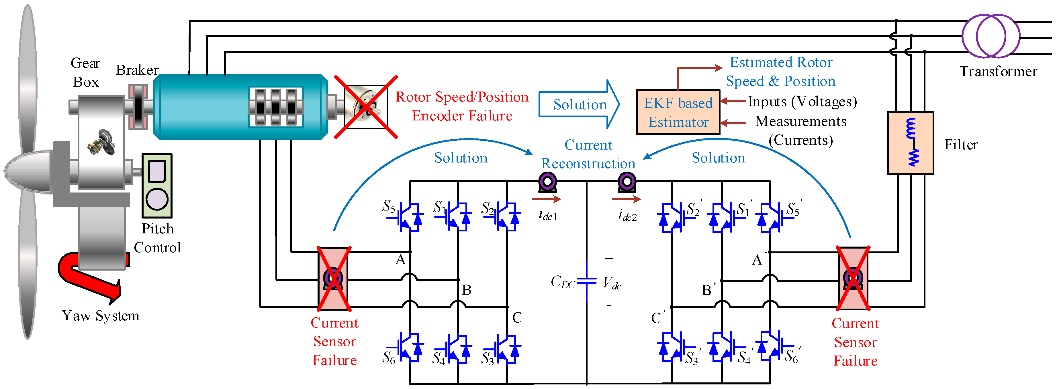
Figure 2.
Prediction and update steps in the extended Kalman filter (EKF) algorithm.
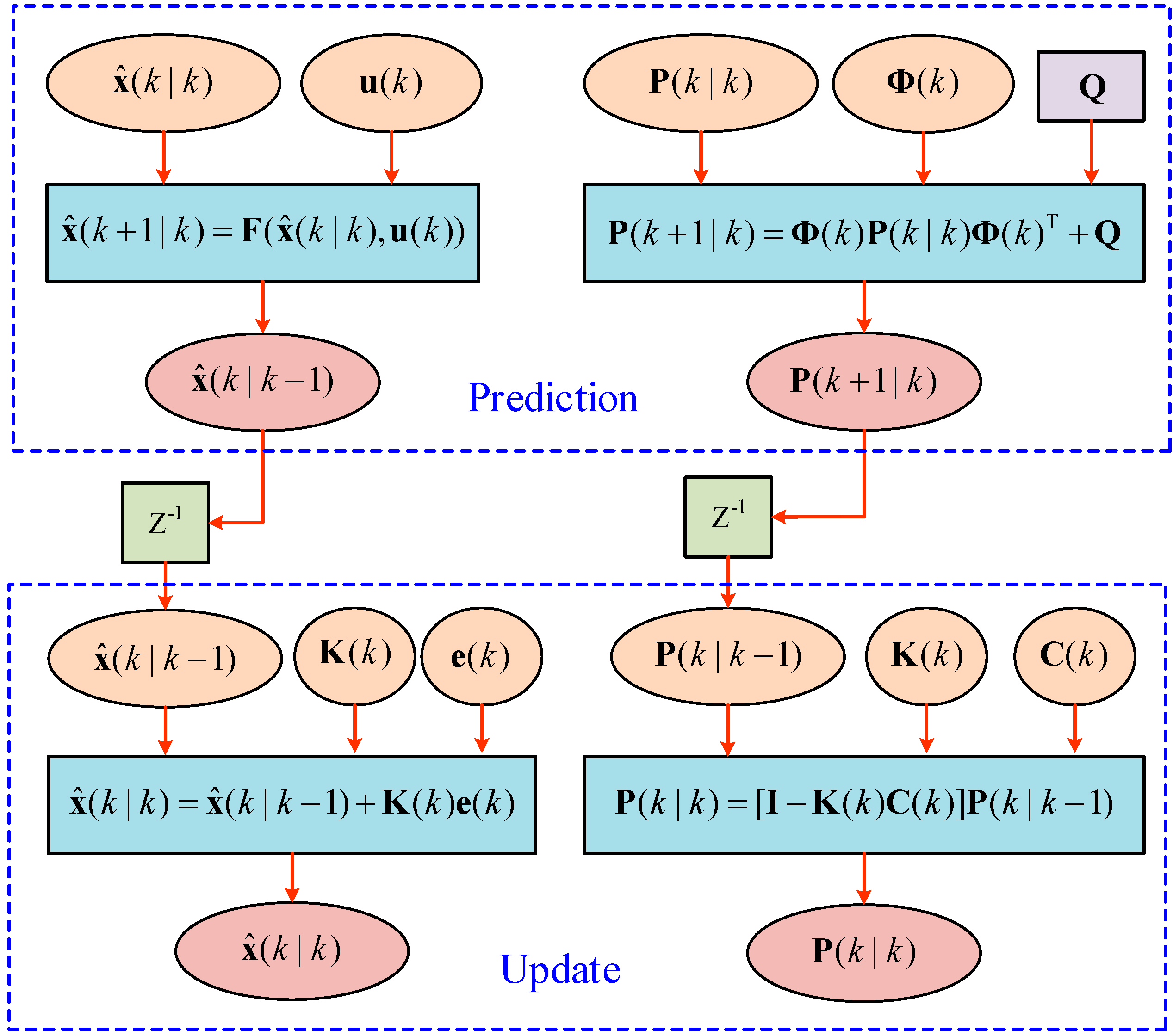
Figure 3.
DC-link current sensor based phase current reconstruction strategy for back-to-back (BTB) of DFIG-WT.
Figure 3.
DC-link current sensor based phase current reconstruction strategy for back-to-back (BTB) of DFIG-WT.

Figure 4.
Space vector distribution for a six-switch three-phase converter.
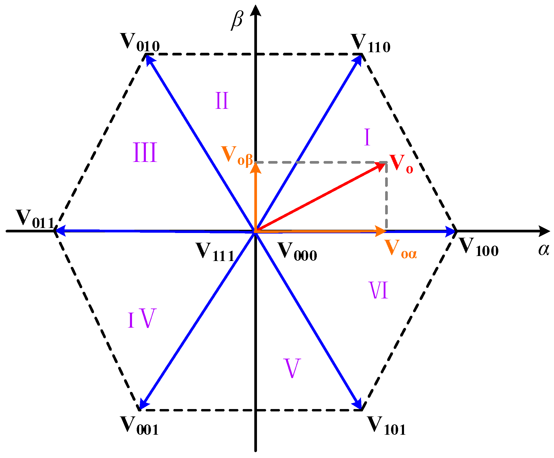
Figure 5.
Sector indicator calculation algorithm.
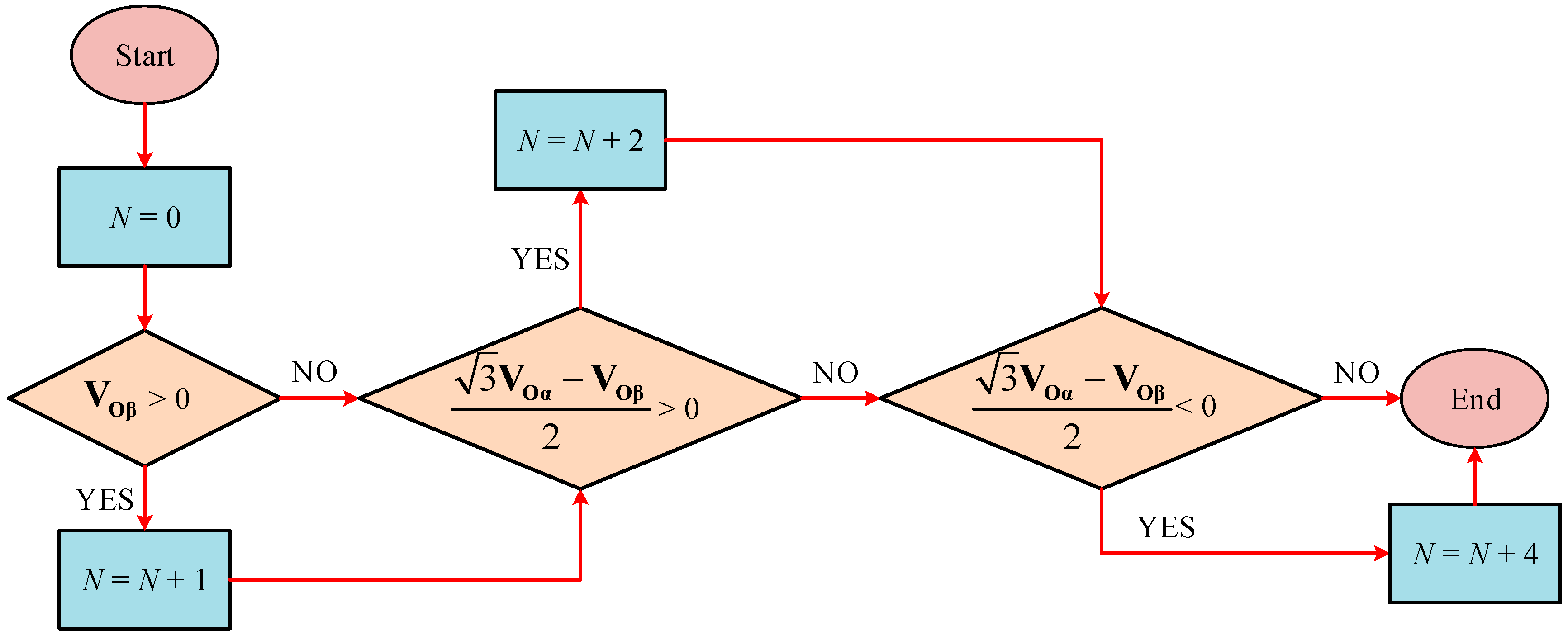
Figure 6.
Switching patterns in different sectors.
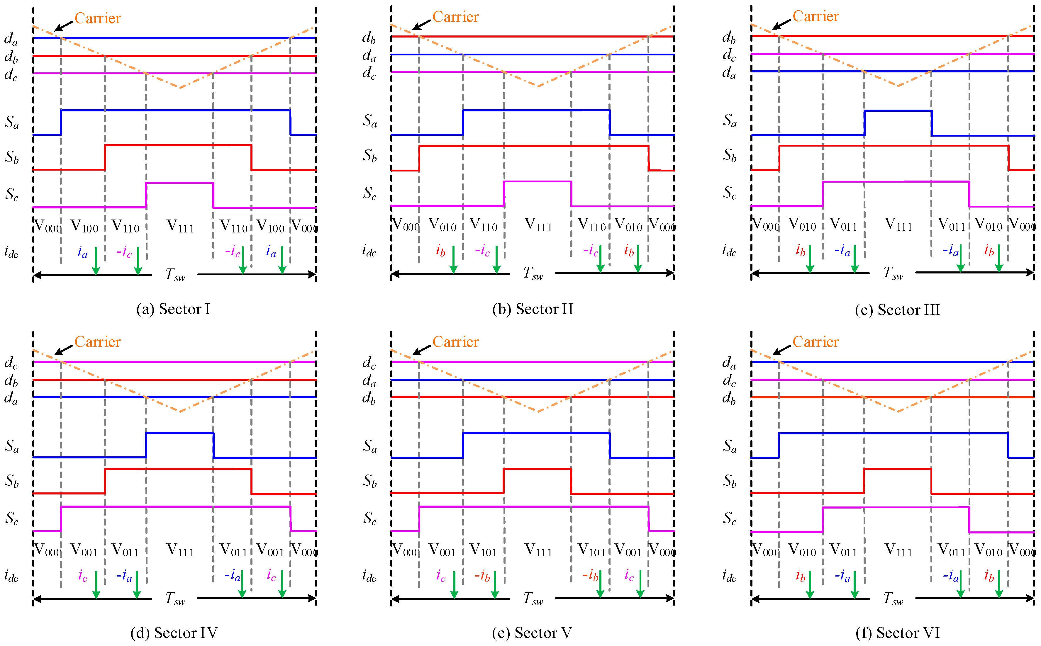
Figure 7.
Ideal and actual current values in the turning on process.

Figure 8.
Three current sampling failure cases in Sector I, when (a) V100 is not available (b) V110 is not available (c) both V100 and V110 are not available.
Figure 8.
Three current sampling failure cases in Sector I, when (a) V100 is not available (b) V110 is not available (c) both V100 and V110 are not available.

Figure 9.
Current reconstruction dead zones and unmeasurable situations in Sector I.
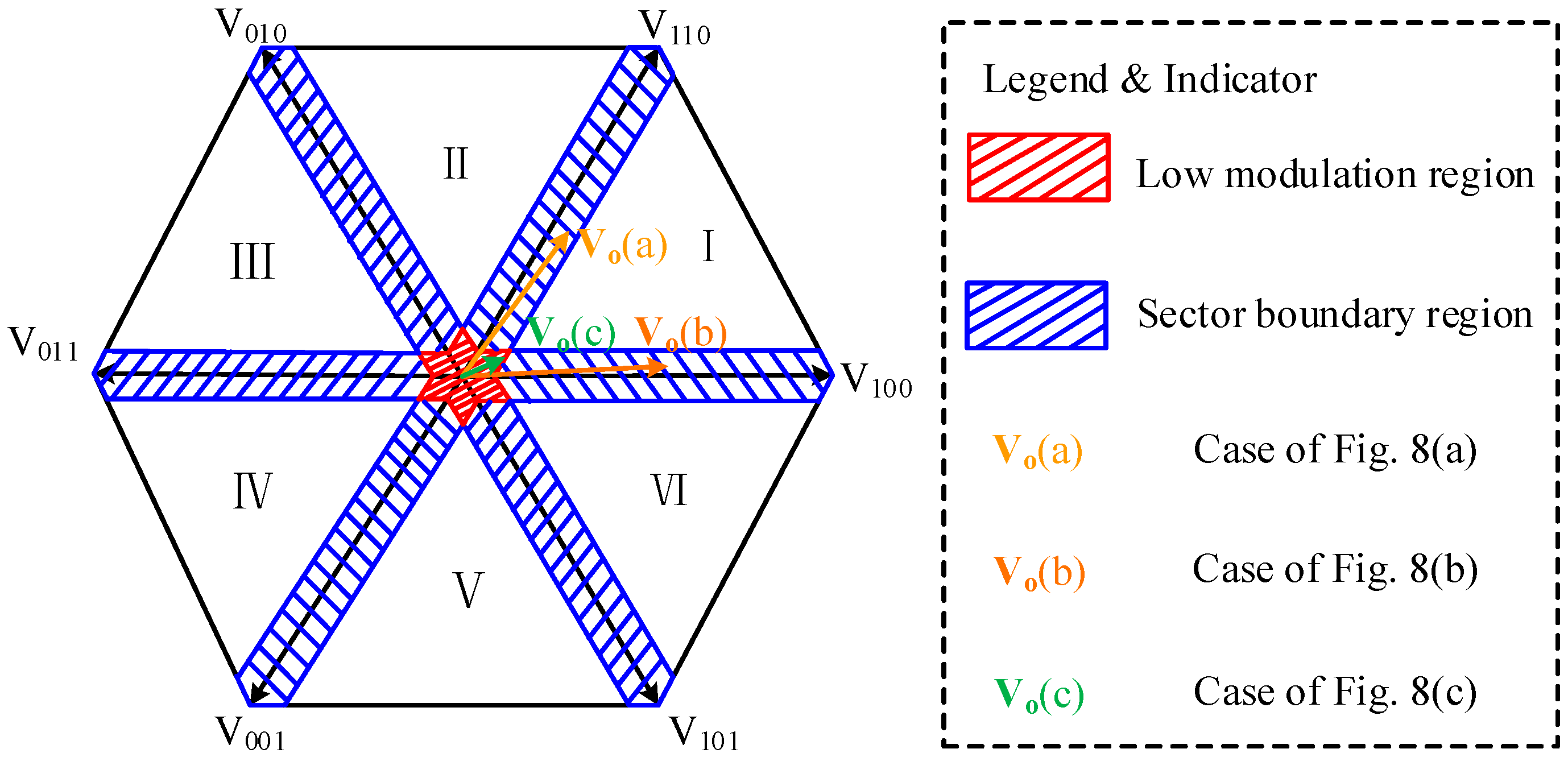
Figure 10.
Relationship between the pulse width and duty ratio difference.
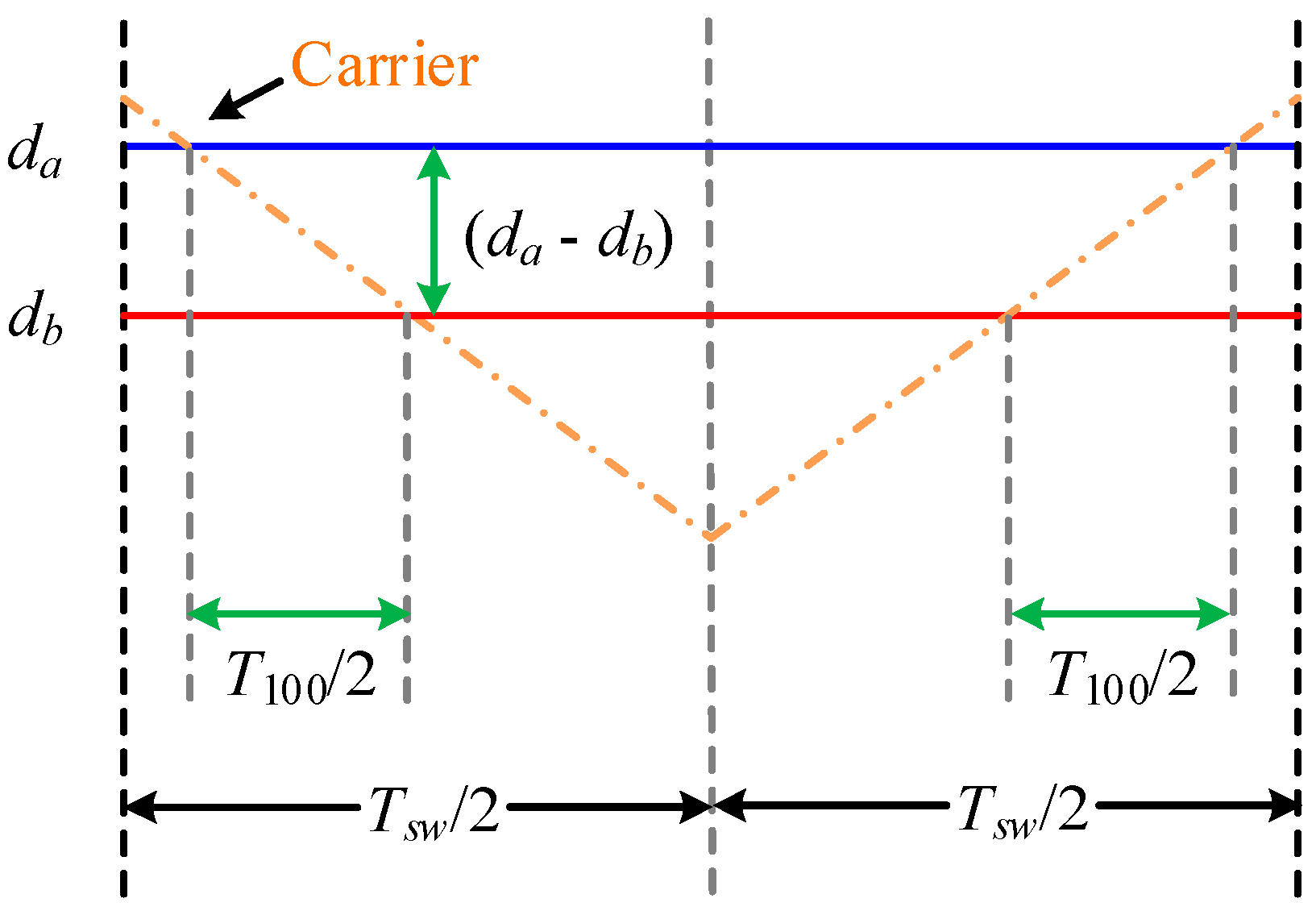
Figure 11.
Space vector allocation with duty ratio adjustment and switching state compensation.

Figure 12.
Hybrid sensorless control strategy for the severe sensor failure scenario in DFIG-WT.

Figure 13.
Wind speed step change at t = 0.5 s.
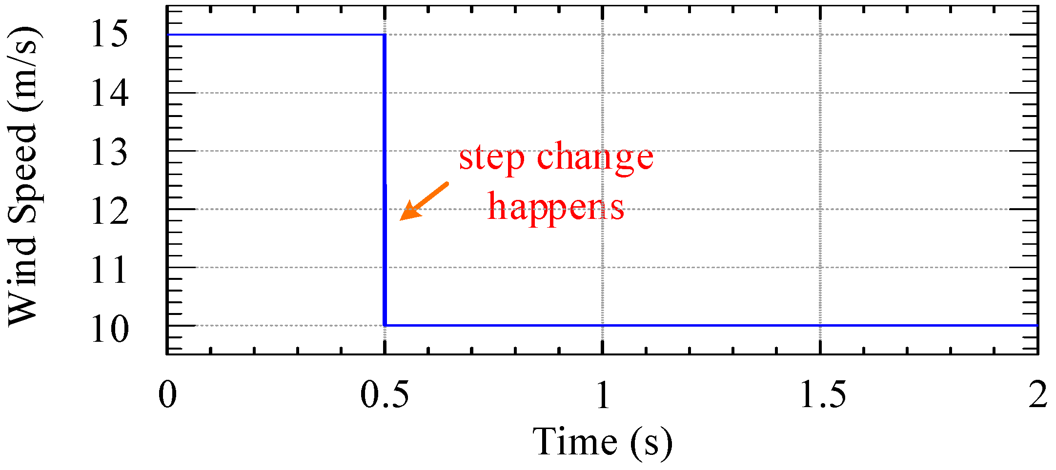
Figure 14.
Three-phase output: (a) voltages; and (b) currents to the AC grid.

Figure 15.
Real and reconstructed three-phase GSC AC currents.
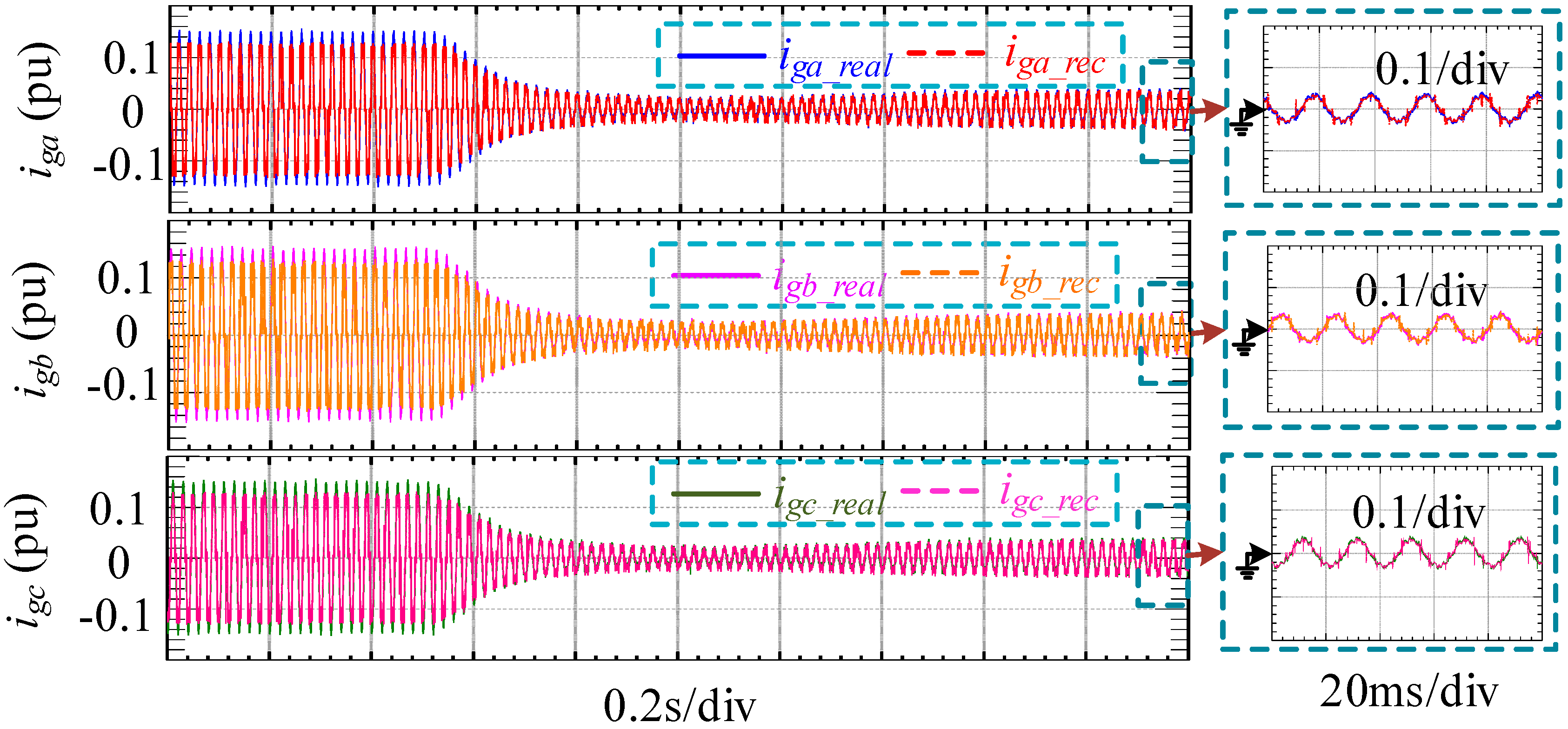
Figure 16.
The total output active power Pt, reactive power Qt and power factor PF under different situations.
Figure 16.
The total output active power Pt, reactive power Qt and power factor PF under different situations.
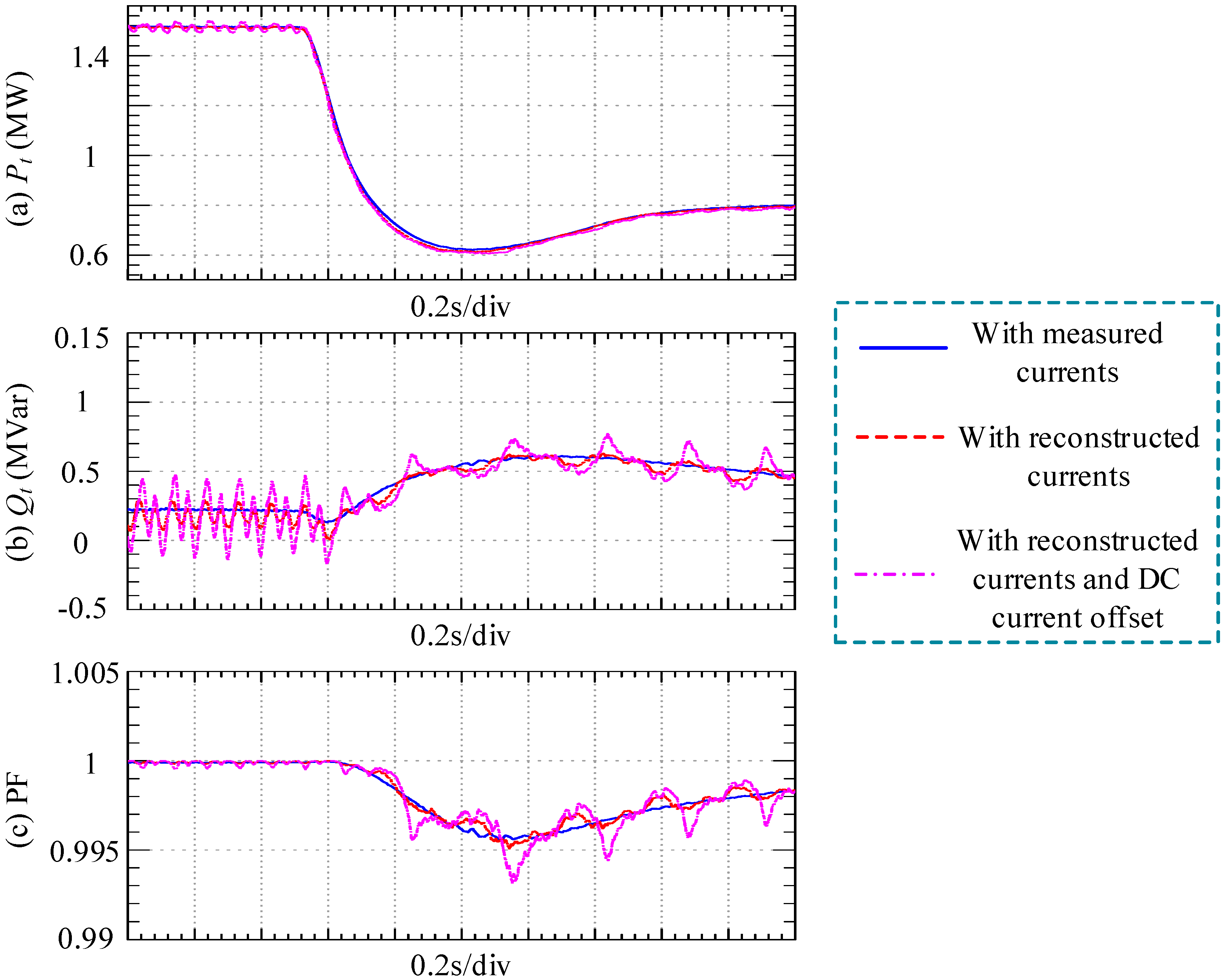
Figure 17.
Real and estimated rotor speeds.

Figure 18.
Real and estimated rotor positions.
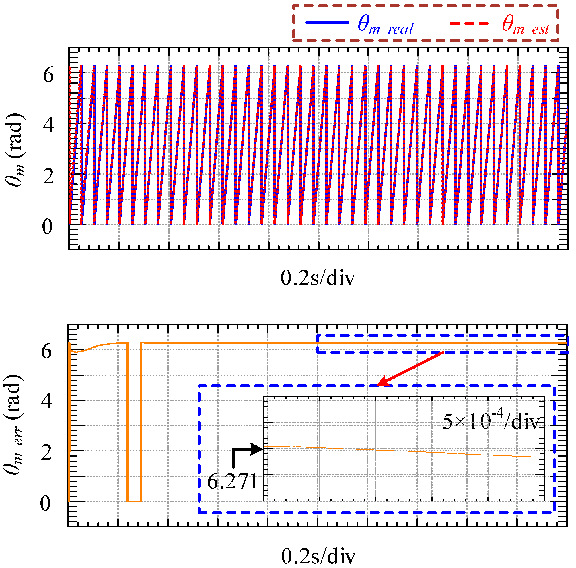
Figure 19.
Mechanical and electromagnetic torques of DFIG-WT.
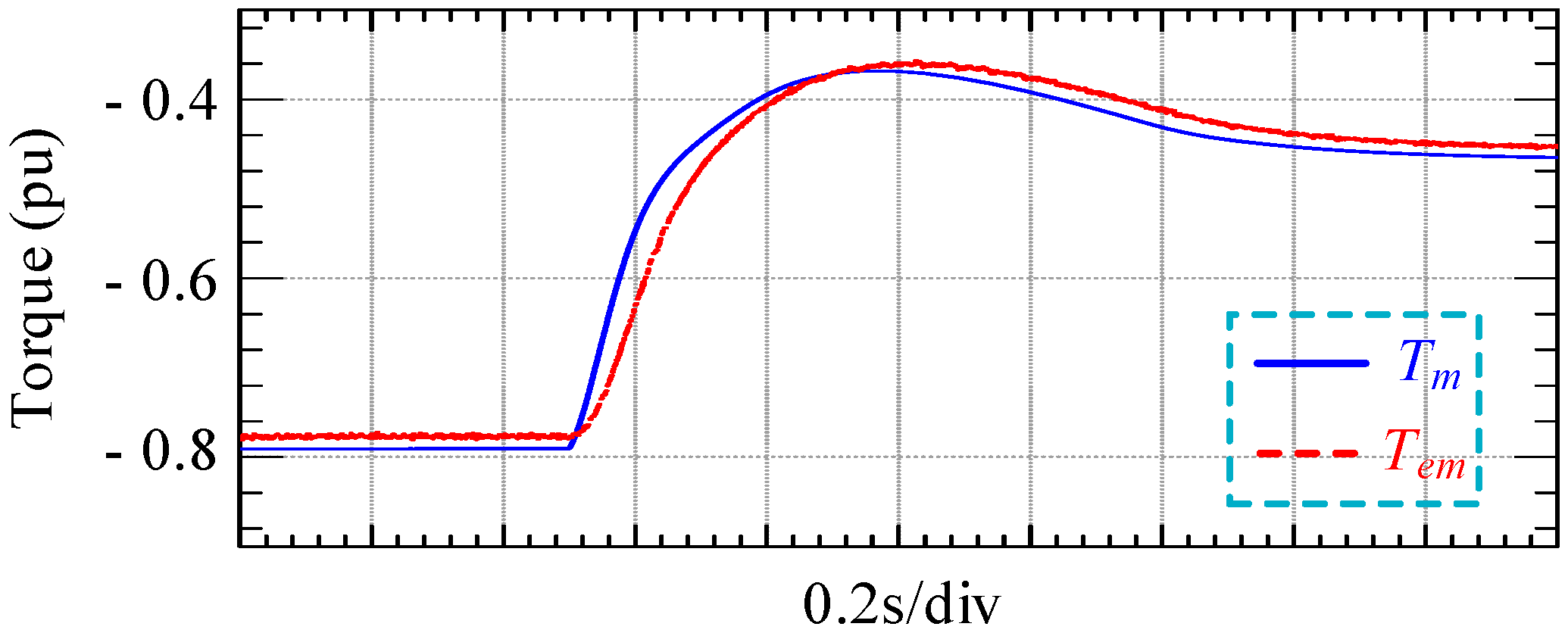
Figure 20.
Real and estimated rotor speeds with noises.
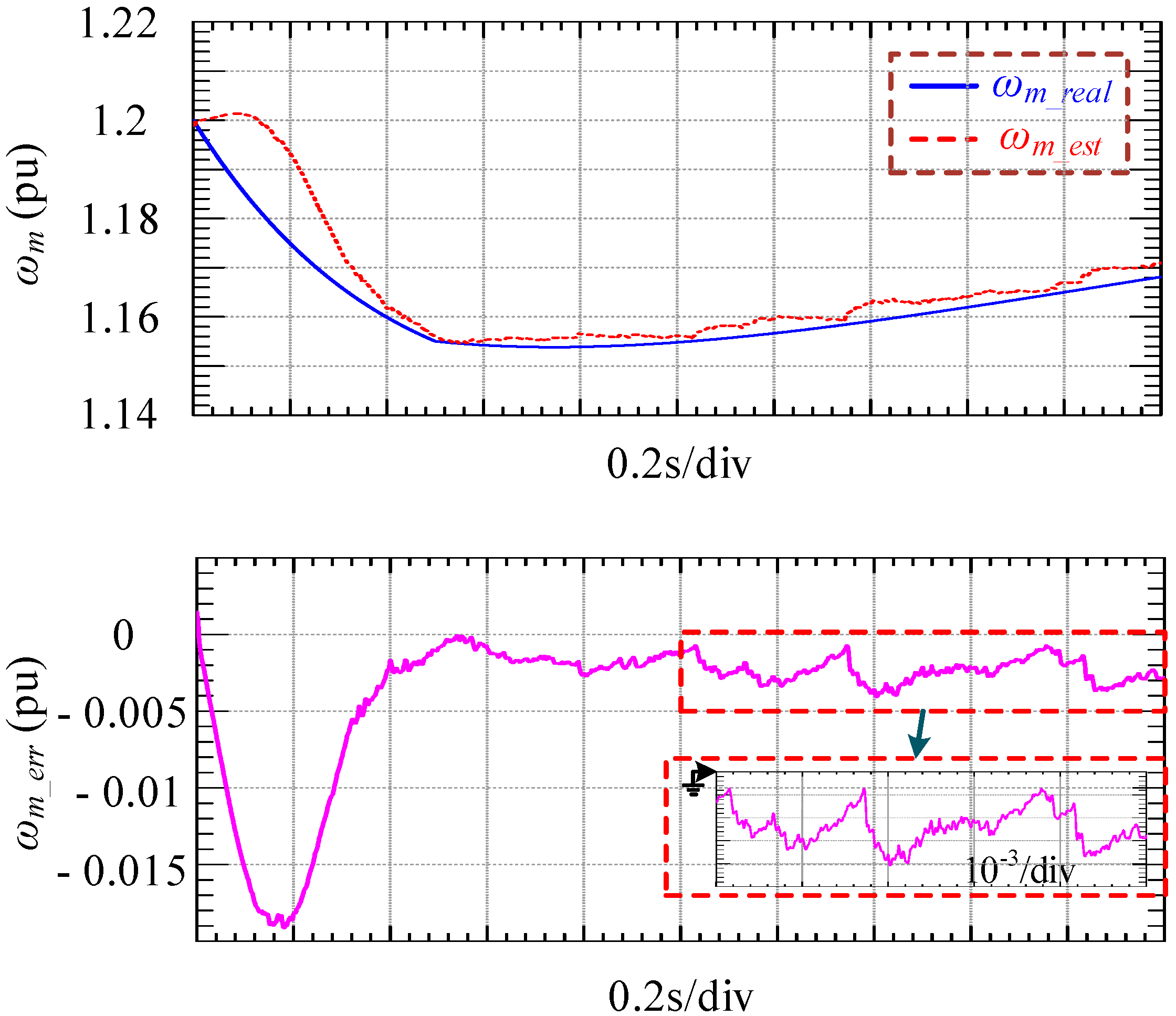
Figure 21.
Real and estimated rotor positions with noises.


Table 1.
Values of parameters c1–c8.
| Parameters | c1 | c2 | c3 | c4 | c5 | c6 | c7 | c8 |
|---|---|---|---|---|---|---|---|---|
| Values | 0.645 | 116 | 0.4 | 5 | 21 | 0.00912 | 0.08 | 0.035 |
Table 2.
Extended Kalman Filter (EKF) algorithm.
| Prediction Step |
|---|
| Update Step |
| Jacobi Matrices |
| Measurement Error |
| Kalman Gain |
Table 3.
Relationships among DC and AC Currents in rotor-side converter (RSC) and grid-side converter (GSC).
Table 3.
Relationships among DC and AC Currents in rotor-side converter (RSC) and grid-side converter (GSC).
| Vabc(a’b’c’) | V100 | V110 | V010 | V011 | V001 | V101 | V000 | V111 |
|---|---|---|---|---|---|---|---|---|
| idc1 | ira | −irc | irb | −ira | irc | −irb | 0 | 0 |
| idc2 | iga | −igc | igb | −iga | igc | −igb | 0 | 0 |
Table 4.
Relationship between N and the sector.
| N | 1 | 2 | 3 | 4 | 5 | 6 |
|---|---|---|---|---|---|---|
| Sector | 2 | 6 | 1 | 4 | 3 | 5 |
Table 5.
Duty ratio adjustment in each sector.
| Sector | Situation | Duty Ratio Adjustment |
|---|---|---|
| I | T100 < Tmin | da + dcom_ab |
| T110 < Tmin | dc − dcom_bc | |
| II | T010 < Tmin | db + dcom_ab |
| T110 < Tmin | dc − dcom_ac | |
| III | T010 < Tmin | db + dcom_bc |
| T011 < Tmin | da − dcom_ac | |
| IV | T001 < Tmin | dc + dcom_bc |
| T011 < Tmin | da − dcom_ab | |
| V | T001 < Tmin | dc + dcom_ac |
| T101 < Tmin | db − dcom_ab | |
| VI | T100 < Tmin | da + dcom_ac |
| T101 < Tmin | db − dcom_bc |
Table 6.
Parameters of DFIG-WT.
| Parameter | Value | Unit |
|---|---|---|
| Rated Power Sg | 1.5 | MVA |
| Rated Frequency Fnom | 50 | Hz |
| Rated Stator Voltage Vs | 575 | V |
| Stator Resistance Rs | 0.023 | pu |
| Rotor Resistance Rr | 0.016 | pu |
| Stator Inductance Lls | 0.18 | pu |
| Rotor Inductance Llr | 0.16 | pu |
| Magnetizing Inductance Lm | 2.9 | pu |
| Friction Factor F | 0.01 | pu |
| Inertia Constant H | 0.685 | s |
| Number of Pole Pairs np | 3 | \ |
| DC Bus Capacitance CDC | 10 | mF |
| Rated Wind Speed vw | 11 | m/s |
© 2017 by the authors. Licensee MDPI, Basel, Switzerland. This article is an open access article distributed under the terms and conditions of the Creative Commons Attribution (CC BY) license (http://creativecommons.org/licenses/by/4.0/).
Share and Cite
MDPI and ACS Style
Li, W.; Li, G.; Ni, K.; Hu, Y.; Li, X. A Hybrid Fault-Tolerant Strategy for Severe Sensor Failure Scenarios in Late-Stage Offshore DFIG-WT. Energies 2018, 11, 21. https://doi.org/10.3390/en11010021
AMA Style
Li W, Li G, Ni K, Hu Y, Li X. A Hybrid Fault-Tolerant Strategy for Severe Sensor Failure Scenarios in Late-Stage Offshore DFIG-WT. Energies. 2018; 11(1):21. https://doi.org/10.3390/en11010021
Chicago/Turabian StyleLi, Wei, Gengyin Li, Kai Ni, Yihua Hu, and Xinhua Li. 2018. "A Hybrid Fault-Tolerant Strategy for Severe Sensor Failure Scenarios in Late-Stage Offshore DFIG-WT" Energies 11, no. 1: 21. https://doi.org/10.3390/en11010021
Note that from the first issue of 2016, this journal uses article numbers instead of page numbers. See further details here.