Remaining Useful Life Estimation of Aircraft Engines Using a Modified Similarity and Supporting Vector Machine (SVM) Approach

1
School of Mechanical and Electrical Engineering, University of Electronic and Science Technology of China, Chengdu 611731, China
2
Department of Mathematics, University of Illinois at Urbana-Champaign, Urbana, IL 61801, USA
*
Author to whom correspondence should be addressed.
Energies 2018, 11(1), 28; https://doi.org/10.3390/en11010028
Submission received: 25 November 2017
/
Revised: 13 December 2017
/
Accepted: 18 December 2017
/
Published: 23 December 2017
(This article belongs to the Special Issue Structural Prognostics and Health Management in Power & Energy Systems)
Abstract
:As the main power source for aircrafts, the reliability of an aero engine is critical for ensuring the safety of aircrafts. Prognostics and health management (PHM) on an aero engine can not only improve its safety, maintenance strategy and availability, but also reduce its operation and maintenance costs. Residual useful life (RUL) estimation is a key technology in the research of PHM. According to monitored performance data from the engine’s different positions, how to estimate RUL of an aircraft engine by utilizing these data is a challenge for ensuring the engine integrity and safety. In this paper, a framework for RUL estimation of an aircraft engine is proposed by using the whole lifecycle data and performance-deteriorated parameter data without failures based on the theory of similarity and supporting vector machine (SVM). Moreover, a new state of health indicator is introduced for the aircraft engine based on the preprocessing of raw data. Finally, the proposed method is validated by using 2008 PHM data challenge competition data, which shows its effectiveness and practicality.
1. Introduction
Recent developments of complex systems, such as aircraft engines, engineering machines, high-speed vehicles and computer numerical control (CNC) systems have been emphasized by the increasing requirements of on-line health monitoring for the purpose of maximizing its operational reliability and safety [1,2,3]. As the core part and power source of aircrafts, the reliable operation of an aero engine is critical for ensuring the reliability and safety of the aircraft, and to maintain its availability, and reduce its maintenance costs [4,5,6]. Among them, prognostics and health management (PHM) is an effective approach and one of the most commonly-used [7,8]. In particular, residual useful life (RUL) estimation is a key technology for PHM. In general, RUL estimation is to indicate the system/component lifetime before it can no longer perform its function, which is also an important way to reduce production loss, save maintenance costs and avoid fatal machine breakdowns of the equipment before its failure [9,10,11,12].
Since the aircraft engine is a complex system, there are various monitored performance data from different positions during its operation. How to estimate RUL of an aircraft engine by utilizing these data has become the focus of most engine industries. Until now, approaches to predict system lifetime can be broadly categorized into three types: physics-based models, data-driven approaches and hybrid approaches [12,13,14]. Generally, a physics-based model utilizes the failure physical model of the system/component to estimate its RUL, which is usually based on the system/component’s physics of failure or physics of dynamics deeply [15,16,17,18,19]. It can usually obtain reasonable and accurate predictions of RUL based on physical models with limited historical data [20]. However, it is usually different or too expensive to apply a physics-based model to a complex system. Besides, this approach has shown significant limitations due to the assumptions and simplifications of the adopted models [21]. The data-driven approach utilizes the monitored operational data relating to system health for RUL estimation [22,23], which is preferred when the system’s failure physics is complicated or unavailable but systems’ degradation procedure and degradation data are available. Note from [3] that the data-driven approach provides accurate RUL predictions for a complex system, which can be applied quickly and cheaply compared to the physics-based model. Furthermore, recent development of sensor technology and simulation capabilities enables us to continuously monitor the healthy situation of a complex system and obtain the related large amount of performance index data. In addition, data-driven approaches can be divided into three categories: statistical techniques and artificial intelligence (AI) techniques. The former includes regression methods such as the auto-regressive and moving average (ARMA) models, and the later includes neural networks and supporting vector machine (SVM), fuzzy logic, etc. The third approach, the so-called hybrid approach proposed by Hansen et al. [24], is the combination of physics-based and data-driven models, in which prognostics results are claimed to be more reliable and accurate, but few studies have been reported [20].
Data-driven RUL prediction models, which are most widely applied in the field of prognostics or PHM, mainly include extrapolation models and statistical models. The extrapolation model is usually used to fit a curve of a system degradation evolution by regression, extrapolate the curve to the failure threshold and obtain the RUL between the current moment and the predicted failure time [25]. The statistical model establishes the relationship between a system’s failure likelihood and its degradation indicator from collected CM (condition maintenance) and failure data [26]. The statistical model approach is classified into the models based on the direct CM data and indirect CM data. The models based on the direct CM data include the proportional hazards model [27,28], proportional covariate model (PCM) [29], Wiener processes, Gamma processes and Markovian-based models. The models based on the indirect CM data include stochastic filtering-based models, covariate-based hazard models and hidden Markov model (HMM) [30], hidden semi-Markov models (HSMM), etc. Statistical models are the most effective ones for RUL estimation when system failure procedure is invisible. Most research has been conducted in RUL estimation based on data-driven models. Stetter and Witczak [31] explored various degradation modeling techniques and how to select the degradation indicator to estimate the RUL. Lee et al. [32] reviewed various methodologies and techniques in PHM research and proposed the systematic PHM design methodology, namely 5S methodology. Moreover, current methodologies of RUL estimation can be summarized as three classes as shown in Figure 1.
Referring to the previous literature and existing methods, a structured form of methodology for RUL prediction is expressed as shown in Figure 1.
When utilizing the data-driven approach for RUL estimation, the whole run-to-failure data of systems are normally needed, but it is difficult to obtain enough run-to-failure data for the long-life systems with high reliability. Thus, it might lead to a large error if the available system history data are lacking. The same problem will arise when the ARMA model is employed. However, if there are some similar systems to the researched system, the failure and performance-deteriorated information of these similar systems are useful for RUL estimation of the researched system. In general, the principle of similarity-based RUL prediction approach is given as follows: if an operating system has similar performance to the reference system during a time range, then assume that they have a similar RUL. Because this reference system is an identical system with the operating system physically, moreover, they operate under the same working conditions and reference systems that have already failed. In addition, if there are more reference systems similar to the researched one, the similarity-based approach can be introduced through a weighted average of the reference systems’ RUL as the researched one’s RUL [33], while the weight is proportional to the similarity between the researched and reference systems. According to this, the similarity-based RUL prediction model gives more reasonable results without modeling the deteriorated process of the researched system. Besides, with the development of PHM, there are abundant historical deteriorated data before failure that could be utilized to perform PHM.
Zio et al. [21] developed a similarity-based approach to predict the RUL by comparing its evolution data to the trajectory patterns of reference samples through fuzzy similarity analysis, and aggregating their time to failure in a weighted sum, which accounts for their similarity to the developing pattern [21]. Gebraeel et al. [22] presents a stochastic process by combining with a data analysis method and deterioration modeling of the components for RUL prediction.
For the traditional similarity-based RUL prediction method, current and past degradation parameters of reference systems have an equal weight when calculating the similarity measure. However, as we all know, a system’s most recent performance to its current health/state is more relative than its earlier performance, and provides more information for its RUL than its earlier performance. Therefore, it is reasonable to assign more weight to a system’s most recent sampling point than its earlier sampling point of performance parameters when measuring its similarity with other systems. However, the traditional similarity-based method ignored this situation. Accordingly, this paper adopts a modified similar-based methodology which introduces a weight-adjusted coefficient to embody the different effect on the calculation of similarity degree from different time ranges while calculating the similarity measure. The more recent sampling point of performance, the bigger weight of the parameter is given. In addition, the earlier value of performance, the parameter is given smaller weight and this paper provides an approach to optimize the weight .
Until now, most research on the similarity-based model for RUL prediction are based on run-to-failure data, but sometimes there are only deteriorated performance data without run-to-failure data. How to utilize these deteriorated performance data, which do not work to failure, to estimate RUL of equipment by similarity-based method, is lacking and expected. Suspension history condition monitoring data usually contain useful information revealing the degradation situation of the system, including environmental factors and loading variations in actual situations, such as degradations and variations of stress amplitudes [10,11,12,34,35]. If these data are properly used, it is helpful to estimate RUL more accurately, particularly when the failure data are insufficient and unavailable in some cases [36,37]. Li et al. [38] used the suspension data to promote the prediction precision of a neural network. However, how to utilize these suspension data to predict RUL of the equipment has not been deeply studied.
This paper attempts to develop a modified similarity and SVM-based method to predict the RUL of an aircraft engine, including two schemes with different reference samples. The first scheme adopts a modified similarity-based method for estimating the RUL of the engine with abundant run-to-failure data of referenced samples, which is named as the modified similarity methodology based on run-to-failure data. The second scheme utilizes deteriorated data of samples without running to failure to estimate the RUL of the operating sample based on SVM and similarity methodology, named as the modified similarity and SVM methodology based on deteriorated data. The structure of this paper is as follows. Section 2 provides a detailed description of two approaches aimed for RUL estimation under two situations. Section 3 introduces how to utilize the proposed approaches to estimate the RUL of an aircraft engine. Section 4 concludes the current research.
2. Proposed Methodology for RUL Estimation
This section is devoted to introducing a similarity-based methodology including two schemes for RUL estimation. The first scheme is to estimate the RUL with abundant run-to-failure data of referenced samples. The other scheme is to estimate the RUL of aircraft engines with some deteriorated data of referenced samples which have no run-to-failure data.
2.1. The Scheme of the Modified Similarity Methodology Based on Run-to-Failure Data
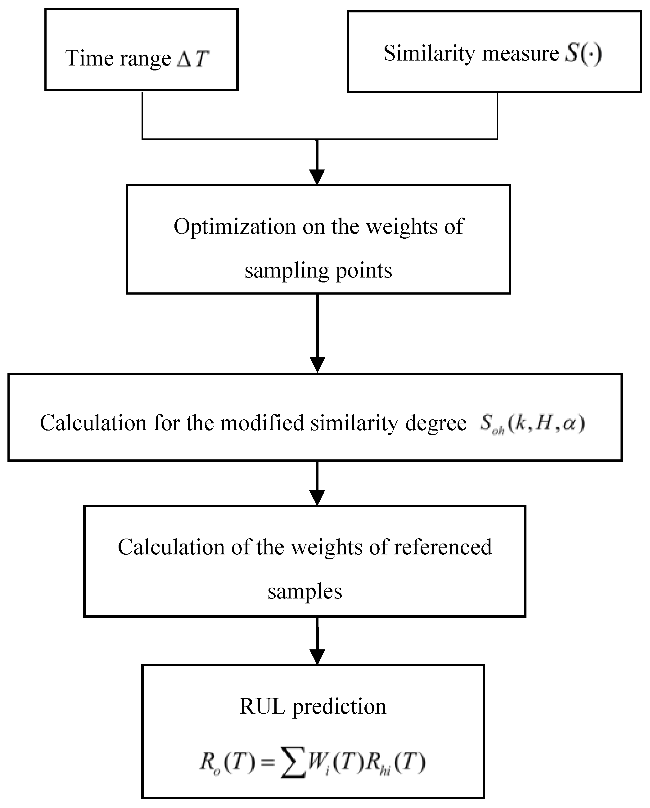
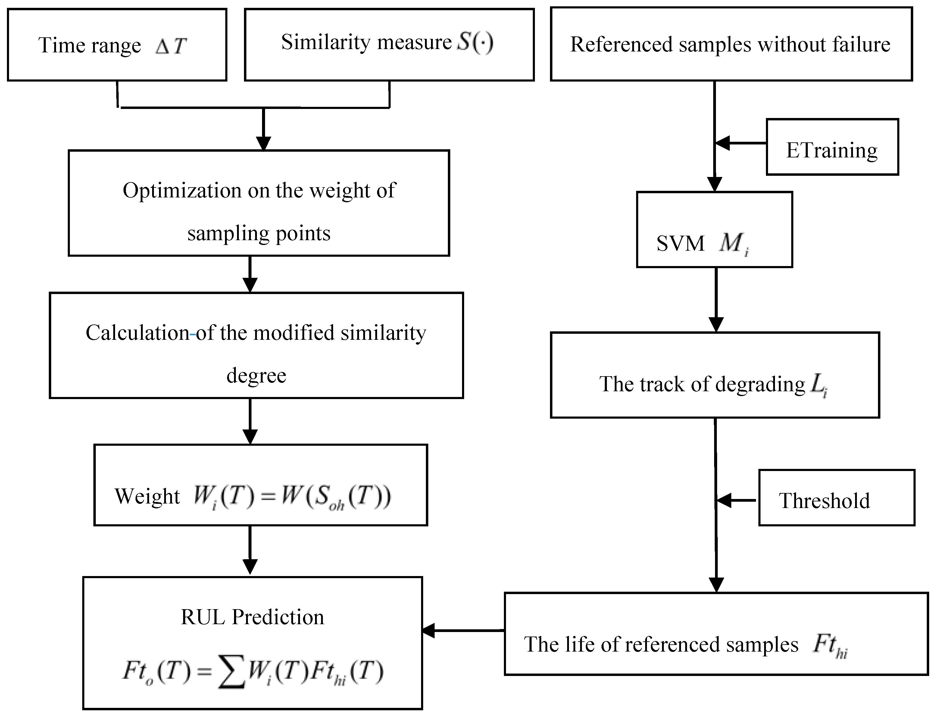
The RUL of an operating sample is the weighted average of RUL of referenced samples. The weights are determined by the similarity degree between referenced samples and the operating one. In particular, the similarity degree is calculated by the weighted average of similarity degrees of sampling points between the reference and operating equipment. This subsection tends to introduce the framework of the modified similarity methodology based on run-to-failure data as shown in Figure 2.
2.1.1. Determination of Time Range for Similarity Measurement
In this analysis, the first step is to set up the time range for similarity measurement, namely, to determine the number of sampling points of the operating system for similarity measurement:
where H is the number of sampling points; represents the time range in which similarity degree between a referenced sample and the operating one; denotes the degradation indicator of the operating sample at the kth sampling point since its operation.
Generally, most of the recent sampling points of the operating system represent its current state. In the traditional similarity-based method, any consecutive sampling points of the condition monitor a reference system before its failure can be used for similarity measurement [15]. In addition, a reasonably long time range can be determined based on operational experience in the lack of prior knowledge. The sampling points in sampling time range are equally considered to be fully representative of the system’s RUL. In this paper, the sampling points of the reference system are confined in the same time range as the operating system, namely, .
2.1.2. Calculation of the Similarity Measure
The second step is to define and calculate the similarity measure, which indicates the similarity degree between the operating and reference systems, and then quantify the degradation duration of the ith reference system that is most similar as the duration of the operating system. The similarity measure S is the function of degradation indicators of the system, which measures the similarity between referenced and operating systems. Note that it may be Euclidean distance, probability function [27] or membership function in fuzzy logic theory [26]. In this paper, the Euclidean distance of degradation indicators between the reference systems and the operating system is introduced as the similarity measure function. The traditional Euclidean distance is expressed as:
where is the similarity measure between the operating system’s degradation process in the time range and reference system’s degradation process in the time range ; where is the failure time of the ith reference system, and . denotes the degradation indicator of the operating system at the sampling point from the sampling point. denotes the degradation indicator of the ith reference system at the sampling point from the sampling point.
The similarity degree between the operating system and the ith reference system at time is defined as:
In this analysis, more weights are assigned to the recent sampling point of degradation indicator than its former sampling points, thus, the Euclidean distance as the similarity measure for illustration is defined as:
where is a weight-adjusting coefficient ranging from 0 to 1. A smaller corresponds to a smaller weight assigned to the former sampling point than recent sampling points of reference systems. can be obtained by optimization for minimal predicting error of operating system’s RUL. An example to obtain is elaborated in Section 3.1.
2.1.3. Definition of the Weight Function
The third step is to define the weight function based on the similarity measure. As aforementioned, the weight is a function of similarity-degree, which is assigned to the reference systems according similarity degree to calculate the RUL of the operating system. The weight of the ith reference system is given by
2.1.4. RUL Estimation of the Operating System
The last step is to estimate the RUL of the operating system. As aforementioned, the RUL of an operating sample at time is the weighted mean value of reference systems at the kth sampling point, and can be obtained by
where n is the number of available reference systems.
The real RUL of the reference system at is , then the operating system’s RUL can be calculated by
2.1.5. Optimization of the Weight-Adjust Coefficient
In order to embody different effects of sampling points of reference systems at different time on RUL estimation of the operating system, the weight-adjust coefficient is introduced in this analysis. The weight-adjust coefficient leads the recent sampling points of reference systems with more weights for the similarity degree calculation, which tends to provide more accurate prediction, specifically, can be obtained by optimization under the goal function
where denotes the first sampling point to deteriorate; is the estimated percentage error at the value of .
2.2. The Scheme of the Similarity and SVM Methodology Based on Deteriorated Data
Research shows that the similarity-based method gives effective and accurate estimation under abundant run-to-failure data of reference samples. However, most equipment operates with high reliability and long life, especially in aerospace applications; the reference samples with enough run-to-failure data are seldom. For this limited or no run-to-failure reference samples, whether the similarity-based method can be used or not needs to be explored. In practices, there is abundant performance deteriorating data and maintenance data during its operating process. These suspension data include useful degradation information relating to the operating system. However, the degradation indicators after halting operating and lifetime of reference samples are unknown since they did not work until failure. Thus, the trend of the degradation indicators and the lifetime of reference samples need to be collected and analyzed. This methodology for RUL estimation consists two essential preprocessing procedures: performance assessment for reference samples and RUL estimation based on reference systems, and then the RUL of the operating system can be derived. In particular, the implementation flowchart is given in Figure 3.
Particularly, SVM is adopted to perform the degradation trend assessment of reference samples and estimate their lifetimes. As is well known, SVM has been commonly used for handling the data of small samples and multiple dimensions. The monitored degradation indicators of reference samples are used to train SVM and obtain the performance-deteriorated pattern of these samples, and fit their relation curve of degradation indicator with time. Based on the curve, the relation function is estimated by using the maximum likelihood estimation method. Once it reaches the failure threshold, the reference systems are considered as failure, so the lifetime of these reference samples can be estimated in this way. The estimated precision regarding the lifetime of these reference systems is the basis for calculating weights of similarity degree. When the estimated precision is higher, the weight assigned to this reference sample is higher. The rest steps are same as that of the modified similarity methodology based on run-to-failure data in Section 2.1.
3. Model Applications to an Aero Engine
This section provides two cases to illustrate the proposed two approaches for RUL estimation of an aero engine.
3.1. The Estimation of RUL for an Airplane Engine with Run-to-Failure Data Though the Modified Similarity Methodology
In this section, the similarity methodology based on run-to-failure data is applied to estimate the RUL of the aircraft engine with multidimensional degraded parameters. The 2008 PHM Data Challenge Competition is introduced for model validation and comparison. The data sets include 21 monitored parameters under 3 different operating modes at a sequence of time, in which three operating modes are flight height (Alt: 0–42 k feet), Mach number (M: 0–0.84) and throttle resolver angle (TRA: 20–100), which reflect the whole operational state of an aero engine. The 21 monitored parameters are different under different operating modes. The raw data of performance parameters from different parts of an aircraft engine is multiple and fluctuated largely without evident regular patterns. It is difficult to estimate the RUL based on these raw data. This paper puts forward a new indicator to characterize the health of the engine based on these raw data. The following section introduces the procedure to obtain the new health indicator.
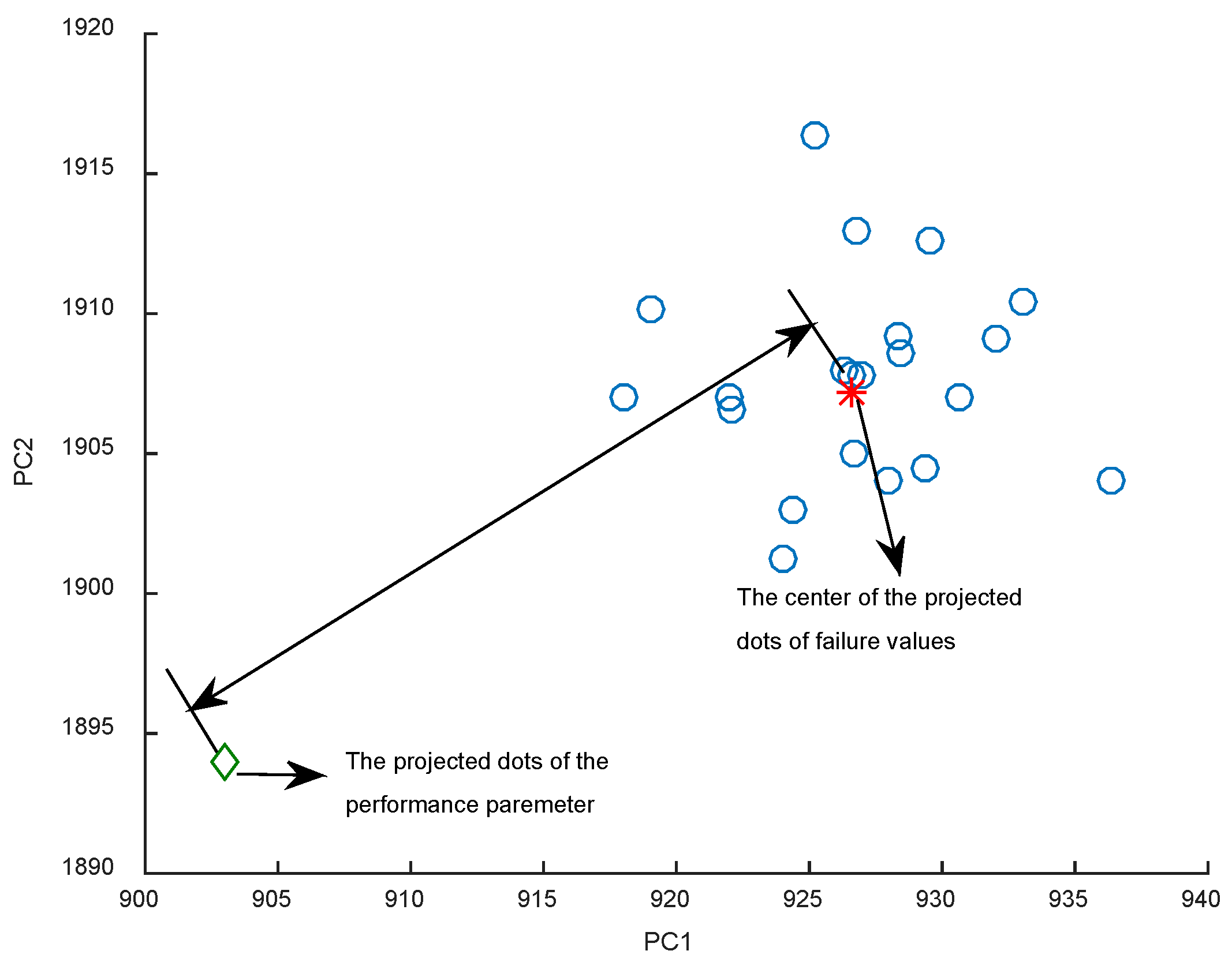
Firstly, the 11 performance parameters that have shown evident changing trend with time are selected after inspecting 21 performance parameters. For the 11 performance parameters, a principal component analysis (PCA) is used to extract the main performance parameters that represent healthy state and degradation trend of the engine system from 11 performance parameters. PCA can reduce the data dimensions. Under different operating modes, the PCA result for 11 parameters is listed as shown in Table 1. Through PCA, the main two-dimensional performance parameters, which occupy more than 98% in all 11 parameters, are derived. Then a new status indicator is established based on the residual two-dimensional performance parameters referring to [22]. The new status indicator is built using the Euclidean distance between the projection of two-dimensional performance parameters at a certain cycle on the failure space and the center of the failure space projection dot in an operating mode.
The detailed steps to construct this healthy status index are shown as follows:
- (1)
- Build the failure space (two-dimensional space) and calculate the projection of the failure values in the failure space, as shown as the hollow dots in Figure 3;
- (2)
- Calculate the center of these projection dots, as shown as star dot in Figure 3;
- (3)
- Calculate the projection dot of the performance parameters on the failure space at a certain cycle;
- (4)
- Calculate the Euclidean distance between the projection dot of the performance parameters in the failure space at a certain cycle and the center of the projected dots in the failure space in an operating mode, which is shown in Figure 4.
Further Euclidean distance means a healthier status of the engine, so this distance is defined as a new healthy status indicator, which represents the engine healthy state and degradation level.
Figure 4 plots the curve of the new health status index of the 196th reference sample. Though this healthy status index shows a certain changing trend, it is still fluctuated intensively. Accordingly, Karman filtering is utilized to further handle this healthy status index. Figure 5 reflects the compared curve of the 196th sample after and before Karman filtering. The red and thick curve is the new degradation indicator of the 196th sample after Karman filtering.
This paper predicted the RUL of five samples No. 196–200 at the 50th cycles, 30th cycles and 10th cycles before failures using the first scheme. An example prediction of the196th samples is given as Table 2.
Firstly, the five sample values from the degradation indicator curve after Karman filtering at every 5 cycles before the 176th cycle are given in Table 2. Then the 10 samples which are most similar with the operated samples are selected as the reference samples according to the new degradation indicator in Equation (1). Time range is , sampling interval is . The weights of these reference samples are calculated by using Equation (4). The results and other information on these 10 reference samples are shown in Table 3.
The predicted RUL of the 196th sample with its actual lifetime 226 cycles are based on these 10 reference samples is given in Table 4. Meanwhile, the estimated RUL of the 196th sample by the traditional similarity method and modified similarity method are compared in Table 4. The weight-adjusted coefficient is preliminarily set as 0.4 in this analysis.
As can be seen from Table 4, the modified method provides better predictions than the traditional one. Moreover, the error by the traditional method increases with time. The prediction precision by the modified method tends to be better when the time is closer to failure. Since the traditional method chooses reference samples that are most similar with the operating sample during a certain time interval in their whole life, the operating sample and this similar reference sample maybe are in different degradation epochs. The modified method constrains the same time range to seek the most similar reference samples. In addition, the modified method assigns larger weight to the more recent sampling point.
Finally, the weight-adjusting coefficient of sampling points is optimized. Through assigning different values to get different predicted precision, the optimized weight-adjusting coefficient value can be obtained at , as shown in Figure 6.
3.2. The Estimation of RUL for an Aero Engine with Deteriorated Data Though the Similarity and SVM Methodology
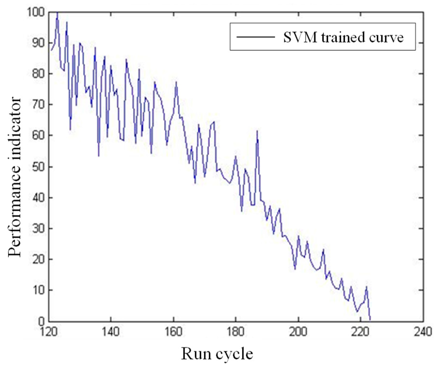
This methodology for RUL estimation includes two essential procedures: assessment for performance of reference samples and RUL estimation of reference samples. The assessment for performance of reference samples is implemented using SVM in this paper. The data are extracted from the same data sets as the previous case, but these whole life data of the original samples are cut off the rear part and only the front part data are applied in this scheme. The degradation indicator pattern of the No. 1 aircraft engine trained by SVM is shown in Figure 7.
The predicted lifetime of all the 20 reference samples by SVM are shown in Table 5. Chi-square test is used to measure the prediction precision, which are used for calculating the weights of reference samples. The No. 11, 13, 18, 17 and No. 3 samples with higher prediction precision are selected to calculate the operating sample’s lifetime as the reference samples. The calculated weights of the reference samples are given in Table 6. The lifetime of No. 196 sample is predicted as shown in Table 7.
It is worth noting from Table 7 that, the proposed methodology has shown better predictions than the traditional one. In particular, the prediction precision is higher when the operational time is closer to the failure point.
4. Conclusions
The RUL prediction of an aircraft engine can not only improve its safety, maintenance, and availability, but also reduce its operation and maintenance costs. This paper presents two schemes to estimate the RUL of an aircraft engine under different situations. The first scheme adopts a modified similarity-based method for estimating the RUL of the aero engine with abundant run-to-failure data of referenced samples. The second scheme utilizes deteriorated data of samples without up-to-failure data to estimate the RUL of the operating sample with less deteriorated performance data than the reference systems. The two schemes are utilized for RUL estimation of an aircraft engine. The model prediction precision shows these two schemes are effective and suitable for RUL estimation of aero engines. More specifically, it is suitable to adopt the modified similarity-based methodology when failed historical samples are abundant and the similarity and SVM methodology is suitable under limited historical samples conditions.
Acknowledgments
The authors acknowledge the support of the National Natural Science Foundation of China (No. 11672070 and 51505067).
Author Contributions
Zhongzhe Chen supervised the projects, and developed the innovative methods and prepared this manuscript. Shuchen Cao and Zijian Mao contributed to the analysis of data, and reviewed and read the final manuscript.
Conflicts of Interest
The authors declare no conflict of interest.
References
- Wang, D.; Peter, W.T.; Tsui, K.L. An enhanced Kurtogram method for fault diagnosis of rolling element bearings. Mech. Syst. Signal Process. 2013, 35, 176–199. [Google Scholar] [CrossRef]
- Zhu, S.P.; Huang, H.Z.; Li, Y.; Liu, Y.; Yang, Y. Probabilistic modeling of damage accumulation for time-dependent fatigue reliability analysis of railway axle steels. Proc. Inst. Mech. Eng. Part F 2015, 229, 23–33. [Google Scholar] [CrossRef]
- Wang, D.; Tsui, K.L. Brownian motion with adaptive drift for remaining useful life prediction: Revisited. Mech. Syst. Signal Process. 2018, 99, 691–701. [Google Scholar] [CrossRef]
- Zhu, S.P.; Huang, H.Z.; Peng, W.; Wang, H.; Mahadevan, S. Probabilistic physics of failure-based framework for fatigue life prediction of aircraft gas turbine discs under uncertainty. Reliab. Eng. Syst. Saf. 2016, 146, 1–12. [Google Scholar] [CrossRef]
- Zhu, S.P.; Yang, Y.J.; Huang, H.Z.; Lv, Z.; Wang, H. A unified criterion for fatigue-creep life prediction of high temperature components. Proc. Inst. Mech. Eng. Part G 2017, 231, 677–688. [Google Scholar] [CrossRef]
- Yu, Z.Y.; Zhu, S.P.; Liu, Q.; Liu, Y. A new energy-critical plane damage parameter for multiaxial fatigue life prediction of turbine blades. Materials 2017, 10, 513. [Google Scholar] [CrossRef] [PubMed]
- Wang, D.; Sun, S.; Peter, W.T. A general sequential Monte Carlo method-based optimal wavelet filter: A Bayesian approach for extracting bearing fault features. Mech. Syst. Signal Process. 2015, 52, 293–308. [Google Scholar] [CrossRef]
- Wang, D.; Tsui, K.L.; Miao, Q. Prognostics and Health Management: A Review of Vibration-based Bearing and Gear Health Indicators. IEEE Access 2017, in press. [Google Scholar] [CrossRef]
- Wang, D.; Peter, W.T.; Guo, W.; Miao, Q. Support vector data description for fusion of multiple health indicators for enhancing gearbox fault diagnosis and prognosis. Meas. Sci. Technol. 2010, 22, 25102. [Google Scholar] [CrossRef]
- Peng, W.; Li, Y.; Yang, Y.J.; Zhu, S.; Huang, H. Bivariate analysis of incomplete degradation observations based on inverse Gaussian processes and copulas. IEEE Trans. Reliab. 2016, 65, 624–639. [Google Scholar] [CrossRef]
- Peng, W.; Li, Y.F.; Yang, Y.J.; Mi, J.; Huang, H. Bayesian degradation analysis with inverse Gaussian process models under time-varying degradation rates. IEEE Trans. Reliab. 2017, 66, 84–96. [Google Scholar] [CrossRef]
- Peng, W.; Shen, L.; Shen, Y.; Sun, Q. Reliability analysis of repairable systems with recurrent misuse-induced failures and normal-operation failures. Reliab. Eng. Syst. Saf. 2018, 171, 87–98. [Google Scholar] [CrossRef]
- Chiang, L.H.; Russel, E.; Braatz, R. Fault Detection and Diagnosis in Industrial Systems; Springer: London, UK, 2001. [Google Scholar]
- Si, X.S.; Wang, W.B.; Hu, C.H.; Zhou, D.H. Remaining useful life estimation: A review on the statistical data driven approaches. Eur. J. Oper. Res. 2011, 213, 1–14. [Google Scholar] [CrossRef]
- Kacprzynski, G.J.; Sarlashkar, A.; Roemer, M.J.; Hess, A.; Hardman, W. Predicting remaining life by fusing the physics of failure modeling with diagnostics. J. Miner. 2004, 56, 29–35. [Google Scholar] [CrossRef]
- Li, C.J.; Lee, H. Gear fatigue crack prognosis using embedded model, gear dynamic model and fracture mechanics. Mech. Syst. Signal Process. 2005, 19, 836–846. [Google Scholar] [CrossRef]
- Zhu, S.P.; Huang, H.Z.; He, L.; Liu, Y.; Wang, Z. A generalized energy-based fatigue-creep damage parameter for life prediction of turbine disk alloys. Eng. Fract. Mech. 2012, 90, 89–100. [Google Scholar] [CrossRef]
- Wang, R.Z.; Zhang, X.C.; Tu, S.T.; Zhu, S.; Zhang, C. A modified strain energy density exhaustion model for creep-fatigue life prediction. Int. J. Fatigue 2016, 90, 12–22. [Google Scholar] [CrossRef]
- Zhu, S.P.; Foletti, S.; Beretta, S. Probabilistic framework for multiaxial LCF assessment under material variability. Int. J. Fatigue 2017, 103, 371–385. [Google Scholar] [CrossRef]
- Ahmadzade, F.; Lundberg, J. Remaining useful life estimation: Review. Int. J. Syst. Assur. Eng. Manag. 2014, 5, 461–474. [Google Scholar] [CrossRef]
- Zio, E.; Maio, F.D. A data-driven fuzzy approach for predicting the remaining useful life in dynamic failure scenarios of an unclear system. Reliab. Eng. Syst. Saf. 2001, 95, 49–57. [Google Scholar] [CrossRef] [Green Version]
- Gebraeel, N.; Lawley, M.; Liu, R.; Parmeshwaran, V. Residual life predictions from vibration-based degradation signals: A neural network approach. IEEE Trans. Ind. Electron. 2004, 51, 694–700. [Google Scholar] [CrossRef]
- Huang, R.; Xi, L.; Li, X.; Liu, C.R.; Qiu, H.; Lee, J. Residual life predictions for ball bearings based on self-organizing map and back propagation neural network methods. Mech. Syst. Signal Process. 2007, 21, 193–207. [Google Scholar] [CrossRef]
- Hansen, R.J.; Hall, D.L.; Kurtz, S.K. New approach to the challenge of machinery prognostics. J. Eng. Gas Turbines Power 1995, 117, 320–325. [Google Scholar] [CrossRef]
- Son, K.; Fouladirad, M.; Barros, A.; Levrat, E.; Iung, B. Remaining useful life estimation based on stochastic deterioration models: A comparative study. Reliab. Eng. Syst. Saf. 2013, 112, 165–175. [Google Scholar] [CrossRef]
- Wang, T.; Yu, J.; Siegel, D.; Lee, J. A similarity-based prognostics approach for remaining useful life estimation of engineered systems. In Proceedings of the International Conference on Prognostics and Health Management, Denver, CO, USA, 6–9 October 2008; pp. 1–6. [Google Scholar]
- Yan, J.; Koc, M.; Lee, J. A prognostic algorithm for machine performance assessment and its application. Prod. Plan. Control 2004, 15, 796–801. [Google Scholar] [CrossRef]
- Roy, A.; Tangirala, S. Stochastic modeling of fatigue crack dynamics for on-line failure prognostics. IEEE Trans. Control Syst. Technol. 1996, 4, 443–451. [Google Scholar] [CrossRef]
- Sun, Y.; Ma, L.; Mathew, J.; Wang, W.; Zhang, S. Mechanical systems hazard estimation using condition monitoring. Mech. Syst. Signal Process. 2006, 20, 1189–1201. [Google Scholar] [CrossRef]
- Gu, J.; Barker, D.; Pecht, M. Prognostics implementation of electronics under vibration loading. Microelectron. Reliab. 2007, 47, 1849–1856. [Google Scholar] [CrossRef]
- Stetter, R.; Witczak, M. Degradation modelling for health monitoring systems. J. Phys. Conf. Ser. 2014, 570, 62002. [Google Scholar] [CrossRef]
- Lee, J.; Wu, F.J.; Zhao, W.Y.; Ghaffari, M.; Liao, L.; Siegel, D. Prognostics and health management design for rotary machinery systems-Reviews, methodology and applications. Mech. Syst. Signal Process. 2014, 42, 314–334. [Google Scholar] [CrossRef]
- You, M.Y.; Meng, G. A generalized similarity measure for similarity-based residual life prediction. Proc. Inst. Mech. Eng. Part E 2011, 225, 151–160. [Google Scholar] [CrossRef]
- Zhu, S.P.; Lei, Q.; Wang, Q.Y. Mean stress and ratcheting corrections in fatigue life prediction of metals. Fatigue Fract. Eng. Mater. Struct. 2017, 40, 1343–1354. [Google Scholar] [CrossRef]
- Zhu, S.P.; Lei, Q.; Huang, H.Z.; Yang, Y.; Peng, W. Mean stress effect correction in strain energy-based fatigue life prediction of metals. Int. J. Damage Mech. 2017, 26, 1219–1241. [Google Scholar] [CrossRef]
- Zhu, S.P.; Liu, Q.; Lei, Q.; Wang, Q.Y. Probabilistic fatigue life prediction and reliability assessment of a high pressure turbine disc considering load variations. Int. J. Damage Mech. 2017, in press. [Google Scholar] [CrossRef]
- Yu, Z.Y.; Zhu, S.P.; Liu, Q.; Liu, Y. Multiaxial fatigue damage parameter and life prediction without any additional material constants. Materials 2017, 10, 923. [Google Scholar] [CrossRef] [PubMed]
- Li, Y.; Billington, S.; Zhang, C.; Kurfess, T.; Danyluk, S.; Liang, S. Adaptive prognostics for rolling element bearing condition. Mech. Syst. Signal Process. 1999, 13, 103–113. [Google Scholar] [CrossRef]
Figure 1.
Methodologies for RUL estimation. RUL: residual useful life; SVM: supporting vector machine; CM: condition maintenance; PHM: prognostics and health management; PCM: proportional covariate model; HMM: hidden Markov model.
Figure 1.
Methodologies for RUL estimation. RUL: residual useful life; SVM: supporting vector machine; CM: condition maintenance; PHM: prognostics and health management; PCM: proportional covariate model; HMM: hidden Markov model.

Figure 2.
Framework for the modified similarity methodology based on run-to-failure data.

Figure 3.
The framework of the similarity and SVM methodology based on deteriorated data.

Figure 4.
Definition of the new health index.

Figure 5.
Trend curve of the 196th sample after and before Karman filtering.
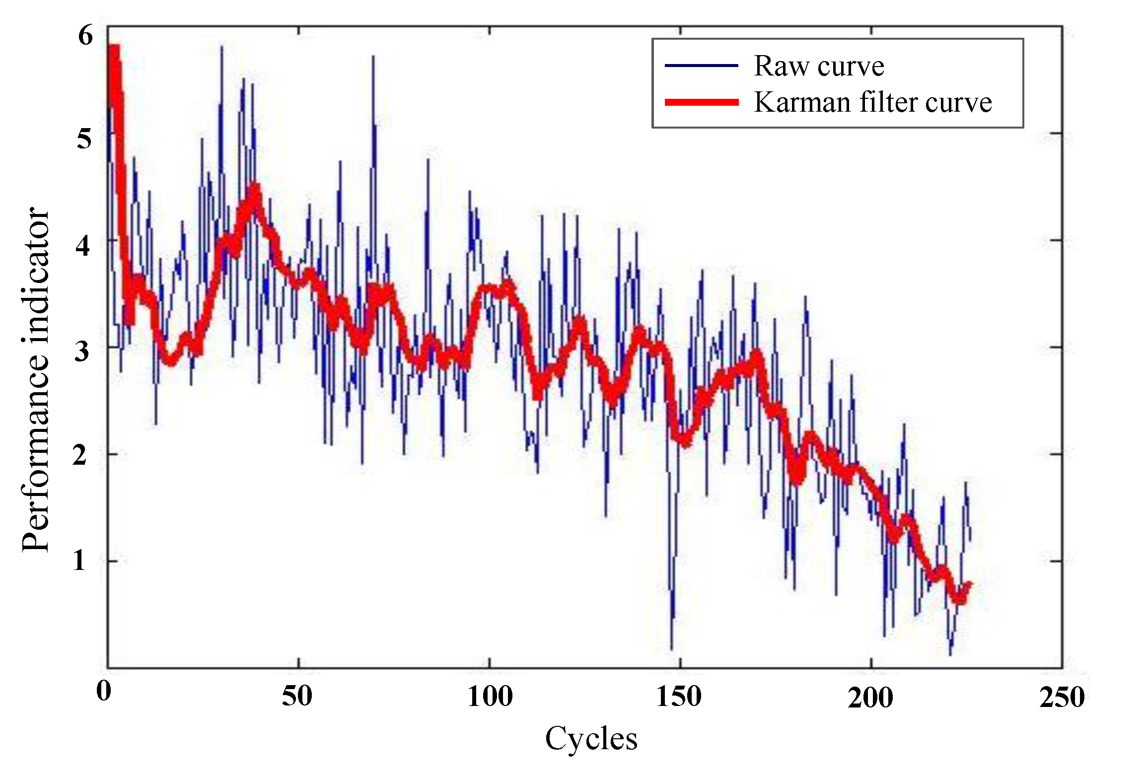
Figure 6.
The MAPE corresponding to weight-adjusting coefficient.
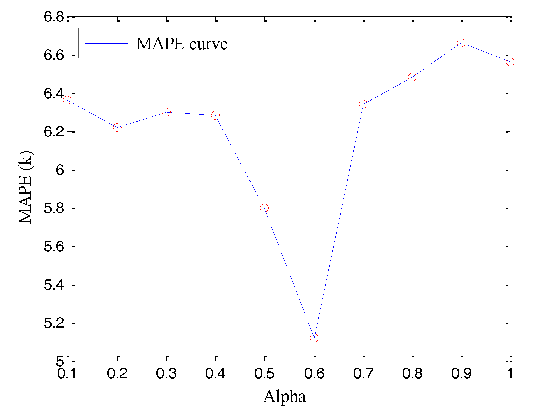
Figure 7.
The SVM trained result of the No. 1 sample.

Table 1.
The detailed occupancy of the main two components in different modes.
| Mode | Mode 1 | Mode 2 | Mode 3 | Mode 4 | Mode 5 | Mode 6 |
|---|---|---|---|---|---|---|
| PC1 | 0.6082 | 0.5892 | 0.7959 | 0.7185 | 0.6087 | 0.5363 |
| PC2 | 0.3803 | 0.4005 | 0.1903 | 0.2641 | 0.3034 | 0.4329 |
Table 2.
The five-sample point of the degradation indicator values of the 196th sample.
| Run Time | 156 Cycles | 161 Cycles | 166 Cycles | 171 Cycles | 176 Cycles |
|---|---|---|---|---|---|
| RUL | 2.5986 | 2.4292 | 2.3260 | 2.4667 | 2.3691 |
Table 3.
Information of the reference samples.
| Ranking | Sample Number | Sampling Interval | Lifetime | RUL | Weight |
|---|---|---|---|---|---|
| 1 | 38 | 224–228 | 287 | 59 | 0.192924 |
| 2 | 82 | 193–197 | 223 | 26 | 0.164397 |
| 3 | 115 | 211–215 | 260 | 45 | 0.162683 |
| 4 | 12 | 120–124 | 242 | 118 | 0.093304 |
| 5 | 29 | 164–168 | 228 | 60 | 0.082048 |
| 6 | 103 | 219–223 | 243 | 20 | 0.080489 |
| 7 | 64 | 122–126 | 154 | 28 | 0.060018 |
| 8 | 53 | 205–209 | 259 | 50 | 0.058619 |
| 9 | 78 | 176–180 | 228 | 48 | 0.055197 |
| 10 | 34 | 244–248 | 286 | 38 | 0.050321 |
Table 4.
RUL estimation of the 196th sample.
| Operating Time | Traditional Similarity Method | Modified Similarity Method | ||
|---|---|---|---|---|
| Predicted RUL | Error (%) | Predicted RUL | Error (%) | |
| 176 | 225.69 | 0.1358 | 214.50 | 5.0871 |
| 177 | 238.11 | 5.3600 | 219.63 | 2.8201 |
| 178 | 213.58 | 5.4953 | 221.18 | 2.1310 |
| 179 | 209.86 | 7.1432 | 219.50 | 2.8742 |
| 180 | 203.53 | 9.9426 | 221.56 | 1.9642 |
| … | … | … | … | … |
| 196 | 197.23 | 12.7305 | 221.62 | 1.9388 |
| 197 | 200.43 | 11.3132 | 219.35 | 2.9427 |
| 198 | 205.42 | 9.1069 | 220.53 | 2.4208 |
| 199 | 200.55 | 11.2619 | 225.75 | 0.1121 |
| 200 | 194.23 | 14.0578 | 226.77 | 0.3401 |
| … | … | … | … | … |
| 216 | 188.03 | 16.8012 | 226.80 | 0.3558 |
| 217 | 184.37 | 18.4209 | 226.17 | 0.0741 |
| 218 | 182.68 | 19.1695 | 225.31 | 0.3036 |
| 219 | 183.04 | 19.0067 | 224.09 | 0.8448 |
| 220 | 181.41 | 19.7290 | 224.15 | 0.8169 |
Table 5.
The predicted lifetime of 20 trained samples.
| Sample Number | Lifetime | ||||
|---|---|---|---|---|---|
| 231.12598 | 289.93651 | 214.7592 | 299.89567 | 372.86392 | |
| 232.23493 | 174.22486 | 290.63039 | 183.51086 | 239.97266 | |
| 214.47475 | 262.17492 | 215.14943 | 238.10682 | 297.89302 | |
| 301.69223 | 236.68347 | 201.39653 | 243.82267 | 255.27005 | |
Table 6.
The weights of the reference samples.
| Reference Samples | W11 | W13 | W18 | W17 | W3 |
|---|---|---|---|---|---|
| Weights | 0.2526 | 0.2258 | 0.1957 | 0.1678 | 0.1581 |
Table 7.
Model predicted lifetime and error of the 196th sample.
| Work Time | Predicted Failure Time | Error (%) |
|---|---|---|
| 121–125 | 201.4377 | 10.86 |
| 126–130 | 189.9478 | 15.95 |
| 131–135 | 188.2144 | 16.71 |
| 136–140 | 187.5556 | 17.01 |
| 141–145 | 188.0059 | 16.81 |
| 146–150 | 192.7102 | 14.73 |
| 151–155 | 203.6575 | 9.88 |
| 156–160 | 227.415 | 0.62 |
| 161–165 | 227.8171 | 0.80 |
| 166–170 | 230.5832 | 2.02 |
| 171–175 | 219.4822 | 2.88 |
| 176–180 | 217.1443 | 3.91 |
| 181–185 | 220.0715 | 2.62 |
| 186–190 | 224.6852 | 0.58 |
| 191–195 | 219.9376 | 2.68 |
| 196–200 | 232.6292 | 2.93 |
| 201–205 | 231.4903 | 2.42 |
| 206–210 | 234.244 | 3.64 |
| 211–215 | 233.7521 | 3.43 |
| 216–220 | 230.2518 | 1.88 |
| 221–225 | 228.2501 | 0.99 |
© 2017 by the authors. Licensee MDPI, Basel, Switzerland. This article is an open access article distributed under the terms and conditions of the Creative Commons Attribution (CC BY) license (http://creativecommons.org/licenses/by/4.0/).
Share and Cite
MDPI and ACS Style
Chen, Z.; Cao, S.; Mao, Z. Remaining Useful Life Estimation of Aircraft Engines Using a Modified Similarity and Supporting Vector Machine (SVM) Approach. Energies 2018, 11, 28. https://doi.org/10.3390/en11010028
AMA Style
Chen Z, Cao S, Mao Z. Remaining Useful Life Estimation of Aircraft Engines Using a Modified Similarity and Supporting Vector Machine (SVM) Approach. Energies. 2018; 11(1):28. https://doi.org/10.3390/en11010028
Chicago/Turabian StyleChen, Zhongzhe, Shuchen Cao, and Zijian Mao. 2018. "Remaining Useful Life Estimation of Aircraft Engines Using a Modified Similarity and Supporting Vector Machine (SVM) Approach" Energies 11, no. 1: 28. https://doi.org/10.3390/en11010028
Note that from the first issue of 2016, this journal uses article numbers instead of page numbers. See further details here.