1. Introduction
PV cells have been extensively studied in the last decades as solar energy is more and more accepted as a viable alternative to traditional energy sources. Rauschenbach [
1] is a reference work, addressing the principles of PV energy conversion. Patel [
2] covers a wider area, dealing both with wind and solar energy. The second edition of the “Handbook of Photovoltaic Science and Engineering” [
3] by Luque and Hegedus is another reference book, providing rich details of all aspects regarding solar energy. Chapter 18 deals with solar cells and modules measurements and models. Aparicio et al. [
4] use free software for modeling PV cells, while Sumathi et al. [
5] and Khatib and Elmenreich [
6] explain how to model a PV cell or array using MATLAB. Honsberg and Bowden [
7] offer an online book with examples, intended for researchers and students, while in another online resource, Van Zeghbroeck [
8] inspects in detail the main information of the semiconductors theory and devices. Modeling the PV behavior is useful for system design, planning, research and training. The goal of this work is to develop an accurate model for a PV cell, expandable to a whole module, using affordable tools and taking into account parameters variations. LTSpice [
9] was chosen as the simulation tool due to its free cost and wide acceptance, Visual Studio Express [
10], also a free tool, was used for parameters estimation and solution validation. Finally, S-Math Studio [
11] was selected for the trial and error different evaluations. The solution implies a reasonable computing power and provides fast convergence. The model itself is portable, as it uses only standard components and is also vendor independent. The input data is usually provided from the manufacturer’s datasheet or can be obtained via experiments.
Unlike other approaches, the model uses the ambient/air temperature and based on the irradiance it calculates the internal (silicon) temperature and provides the actual values of the parameters.
The paper is organized as follows:
Section 2 briefly analyzes the classical PV model and its equations.
Section 3 deals with the information provided by the PV cell datasheet and the equipment involved in measurements. Finding the solution for the PV cell model is analyzed in
Section 4, with
Section 4.1 introducing the solving algorithm. A review of parameters variation is the subject for
Section 4.2, including the real operating conditions, when the PV solar cell is self heating. The new PV cell model is proposed in
Section 4.3, the experimental results are exposed in
Section 5, while conclusions are presented in
Section 6.
2. The Classical PV Cell Model
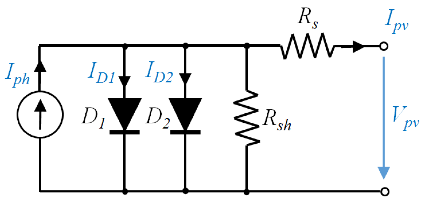
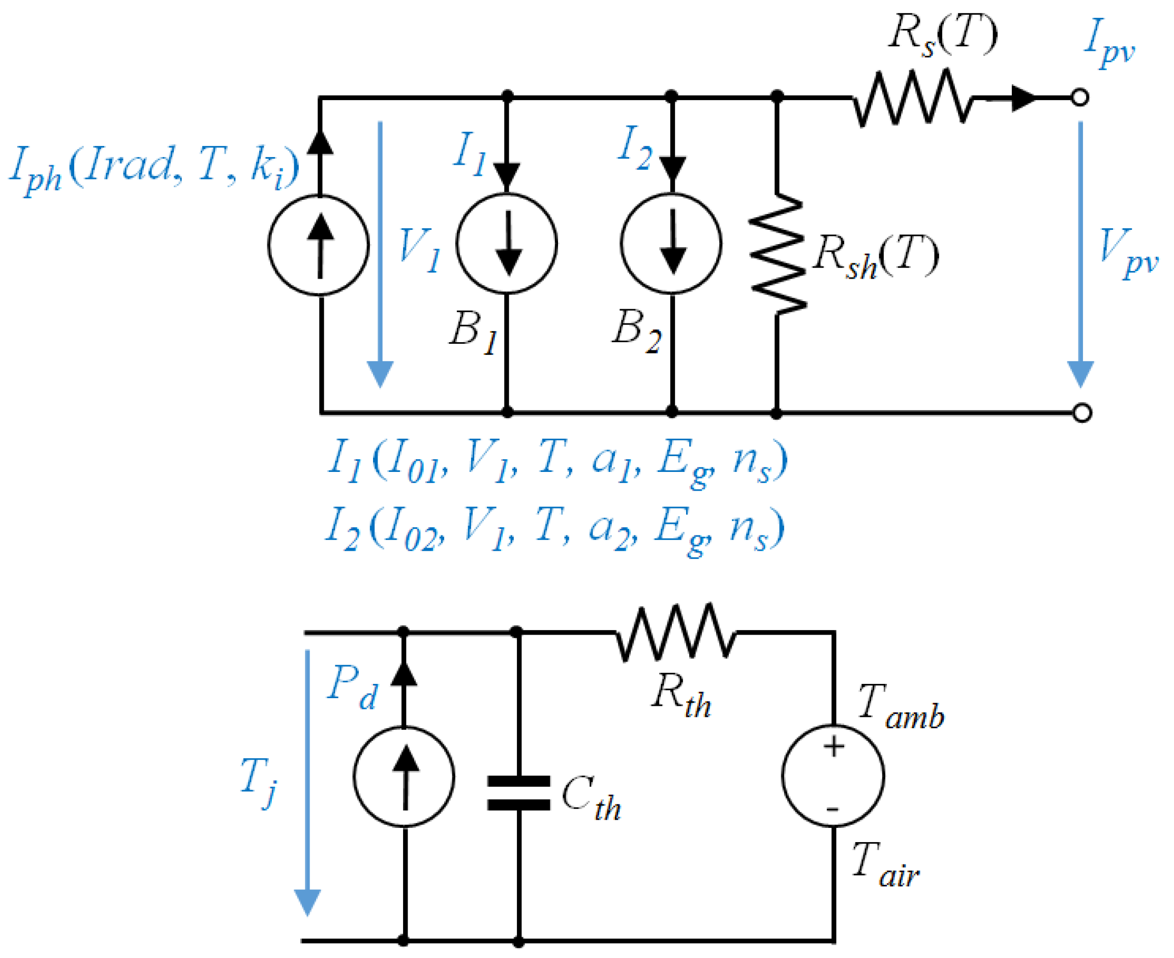
The equivalent circuit of a solar cell is investigated in many prior works. It is generally accepted that a PV cell can be modeled by the circuit in
Figure 1, including one [
12,
13,
14,
15,
16,
17,
18,
19,
20,
21,
22,
23,
24,
25,
26,
27,
28,
29,
30,
31,
32], two [
33,
34,
35] and rarely three or more diodes [
36,
37]. Erdem and Erdem [
38] propose a distance learning experiment for a PV cell model using MATLAB. In [
12], Green focuses on fill factor formulae. Phan and Chan [
13] are among the first who provide an analytical solution for a PV model. However, they do not consider parameters variation and have a limited range for
. Further proposals for PV models can be found in [
14,
15]. Walker [
16] uses a MATLAB PV model to study MPPT converter technologies. De Blas et al. [
17] and Xiao et al. [
18] further enhance the PV models adding new perspectives, while King et al. [
19] propose a model available online using an extensive set of experimental data. De Soto et al. [
20] propose a model for a PV array, while Schlosser and Ghitas [
21] analyze the AC parameters of the PV cell.
Villava et al. [
22] develop an accurate algorithm for finding the PV model parameters at the reference temperature. Kim et al. [
23] concentrate on transient analysis based on a grid-connected PV system. Di Piazza and Vitale [
24] investigate different shadowing conditions. A model dedicated to monocrystalline PV panels is proposed by Jung and Ahmed [
25]; Kim and Choi [
26] introduce an interesting way for finding the PV cell parameters. Advanced mathematics is used in [
27] for the same purpose while Saloux et al. [
28] elaborate explicit parameters finding around MPP. Further models are also proposed by Cuce [
29] and Tian et al. [
30].
Cubas and Pindado [
31] use Lambert W-function for PV cell parameters extraction and they also provide an LTSpice model based on these parameters. In a recent paper, Aller et al. [
32] propose an estimation of the PV parameters that can used in inverters power control.
Chan and Phang [
33] do a pioneering work in establishing a solution for the double diode PV model with the assumption of the ideality factor being 1 for the first diode and 2 for the second diode. Sandrolini et al. [
34] extract the double diode model parameters using a numerical method by cluster analysis, while Ishaque et al. [
35] address the same problem using a MATLAB model, able to correctly operate also on shading conditions.
In
Figure 1,
current source models the photo generated current, with a linear dependency on the irradiance. The first diode,
, is associated with the diffusion mechanism. The second diode,
, is inserted to include the effect of charge recombination. Resistance
represents the cell series resistance and resistance
the cell parallel (shunt) resistance. Resistance
is related to the losses in cell solder bonds, wires, junctions and so on and it is usually bellow 1 Ω. Resistance
is related to the leakage current through the high conductivity shunts across the p-n junction and its order starts in the order of ten of ohms to several kΩ. The circuit in
Figure 1 can be extended to any combination of
series—
parallel cells within a PV module (array). In this paper we shall consider only one diode in the model,
, neglecting
. The equations will be provided in a general form, while the simulations and the experiments will be conducted for a single cell, that is for
. In the remaining text, for simplicity reasons, the output cell voltage
and the output cell current
will be written as
and
, respectively.
Referring to
Figure 1, according to Kirchhoff’s current law (KCL), one can write:
where
is the diode reverse saturation current,
is the electron charge,
is the Boltzmann constant,
is the actual silicon temperature and
is the ideality factor of the diode.
Current
linearly depends on irradiation and temperature [
15,
18]:
At the maximum power point, using (1), the maximum power
can be derived [
22]:
Even in (1) and (3)
is considered equal to
, a more accurate formula for
is [
22]:
A good overview of the PV cell performance can be found in [
12], where an empirical formula for the fill factor
is introduced, considering the single diode model:
3. Materials, Methods and Equipment
For our experiments we have chosen a high efficiency low cost monocrystalline Silicon PV solar cell, unmounted in panels [
39]. The datasheet of the PV cell offers a limited amount of data, summarized in
Table 1.
It is important to note that for any solar cell. This is a good starting point for any simulation or MPPT algorithm implementation.
The data from the datasheet is confusing, as:
The claimed maximum power (5.21 W) differs from . This latter value will be considered subsequently.
The claimed fill factor (81.90%) differs from the standard definition .
The empirical Equation (5) yields an approximate result (
) when compared to the datasheet values (
Table 1).
The irradiance was measured with a Klipp and Zonen SHP1 pyrheliometer with integrated temperature sensor for temperature compensation. The internal silicon temperature was determined with a FLIR E8 infrared camera and a PT1000 temperature sensor on the rear of the PV cell. In order to obtain reliable data, the PT1000 temperature sensor was glued with high thermally conductive adhesive to the backside metal coating of the PV cell. The ambient temperature was measured using the National Instruments NI USB T01 interface. Due to the extremely low internal series resistance , several series cells were carefully wired and a Kelvin connection had to be used for voltage measurements. The measurements were performed under real life conditions, when the solar irradiance was maximum with the PV cells oriented toward the sun on 45 degree inclined support. The load was an ET Instrument ESL-Solar, configured in MPPT mode.
The accuracy of the irradiance measurement relies on the Klipp and Zonen SHP1 pyrheliometer with zero offset due to temperature change, temperature dependence of sensitivity below 0.5% from −30 to +60 °C and nonlinearity below 0.2% for up to 1000 W/m2 irradiance. The accuracy of the temperature sensor for the ambient temperature and PV cell backside coating is 0.6 °C in the measurement range of 0–60 °C. The FLIR E8 infrared camera has an accuracy of 2 °C with thermal sensitivity below 0.06 °C. The accuracy of the FLIR infrared camera is lower than the measurements taken with the temperature sensors but offers the advantage of contactless measurement which is important for PV cell front side measurements. However, the existence of hot spots can be easily observed with this method. The electrical noise was minimized using the following digital busses for communication: Modbus for irradiance and PV cell back side temperature measurement, USB for ambient and PV cell front side temperature measurements.
4. Classical Model Solving
Several ways for solving the equations have been proposed. In [
17] de Blas et al. assume the operation of a solar module at high irradiance levels and deduce the parameters accordingly. De Soto et al. [
20] show how the values of parameters for the five-parameter model can be determined for four different cell technologies. The methods introduced in [
22,
26] are somehow similar, the parameters being precisely extracted by letting the resistance values converge to the actual value in repeated numerical loop computations. Ishaque and Salam [
27] use the differential evolution for parameters extraction. Saloux et al. [
28] introduce a model able to predict the short-circuit current, the open-circuit voltage and the maximum cell power. Tian et al. [
30] concentrate on an extension of the PV cell model for modules and arrays, for monocrystalline and polycrystalline silicon, used for shading effect investigation under different operating conditions.
One of the difficulties is the implicit nature of Equation (1) regarding
. This has been addressed by various techniques, ranging from pure mathematical approaches (including Lambertian W-Function, [
31]) to pure numerical solutions, mainly in MATLAB [
5,
6,
16,
35].
Later models take into account the parameters variation with temperature and irradiance. Radziemska and Klugmann [
40] analyze the temperature influence on the I-V curves of the PV cell, while Tsuno et al. [
41] include also the irradiance in the analysis. Singh et al. [
42] also present the temperature influence, while Cuce and Bali [
43] focus on parameters variation in humid climates. The Lambert W-function is again used by Ghani and Duke [
44] to estimate the parasitic resistances of the PV cell. The correlation between the temperature and PV cell efficiency is addressed in [
45,
46]. Temperature and irradiance influence on the PV cell characteristics via experiments is presented in [
47,
48]. Araneo et al. [
49] propose a model to predict the PV cell temperature based on date, time and geographical position. Temperature and irradiance influence are also investigated in two recent papers by Chander et al. [
50] and Aller et al. [
51]. However the most common approach considers the internal PV temperature as an independent parameter and plots the I-V family curves for different temperatures. This aspect will be covered in the subsequent sections. It has to be stressed out that the exponential nature of Equation (1) determines that a small variation in any of the terms involved in the exponential term to substantially modify the final result. This aspect will be addressed in
Section 5 and
Section 6.
4.1. Solving the Equations for the Classical PV Model
The method introduced here is an extension of the method proposed by Villalva et al. [
22] and involves the following steps:
Compute
For validation purposes determine the limits and
For all values between with as increment, numerically solve (1) for the MPP.
When the maximum power error is below the imposed threshold error, is established and can be computed.
A VB.net application has been developed by the authors in order to numerically solve and compute the model parameters. The application can be downloaded from
http://tess.upt.ro.
Figure 2 depicts a print screen for the initial parameter passing (a) and the results (b).
In our case, using the values taken from the datasheet for
, it results that:
These limits are important to set reliable ranges for the algorithm. The final results are listed in
Table 2.
Several attempts have been made for finding explicit expressions for
and
based on actual datasheet data. For example, Cubas et al. [
31] offer the
formula (with
as an argument, considering
):
For the above data, the formula (8) yields a result of 59.43 Ω, compared to the actual value of 73.19 Ω.
In a simplified model (
), Xiao et al. [
18] propose for
the following relationship (again
):
Here (9) yields mΩ, quite far from its actual value (3.8 mΩ).
4.2. Parameters Variation for Different Conditions
The parameters in Equations (1)–(4) are not constant over the environmental conditions, as depend on temperature and irradiance. A brief review of these dependencies is provided bellow.
4.2.1. Diode Saturation Current—
Phang et al. [
13] show that if
is below 10 A,
can be derived as in (10):
in (10) yields a very good result of 1.3969 nA vs. 1.39427 nA obtained in
Table 2.
Gow and Manning [
15] were among the first to claim that:
The temperature dependence of this current is more detailed expressed by [
16,
20]:
where
is the bandgap voltage of the semiconductor (
V for Si at 25 °C).
can be derived from (1) at the reference temperature as:
According to Vilalva et al. [
22],
can be further improved:
In subchapter 4.6.3 of [
8], Van Zeghbroeck states an equation in which
can be derived from, that can offer an alternate way to estimate
:
This proves to be not very accurate in our case, as with the values from
Table 1,
from (15) results 0.085 nA, quite far from the actual value (1.39427 nA).
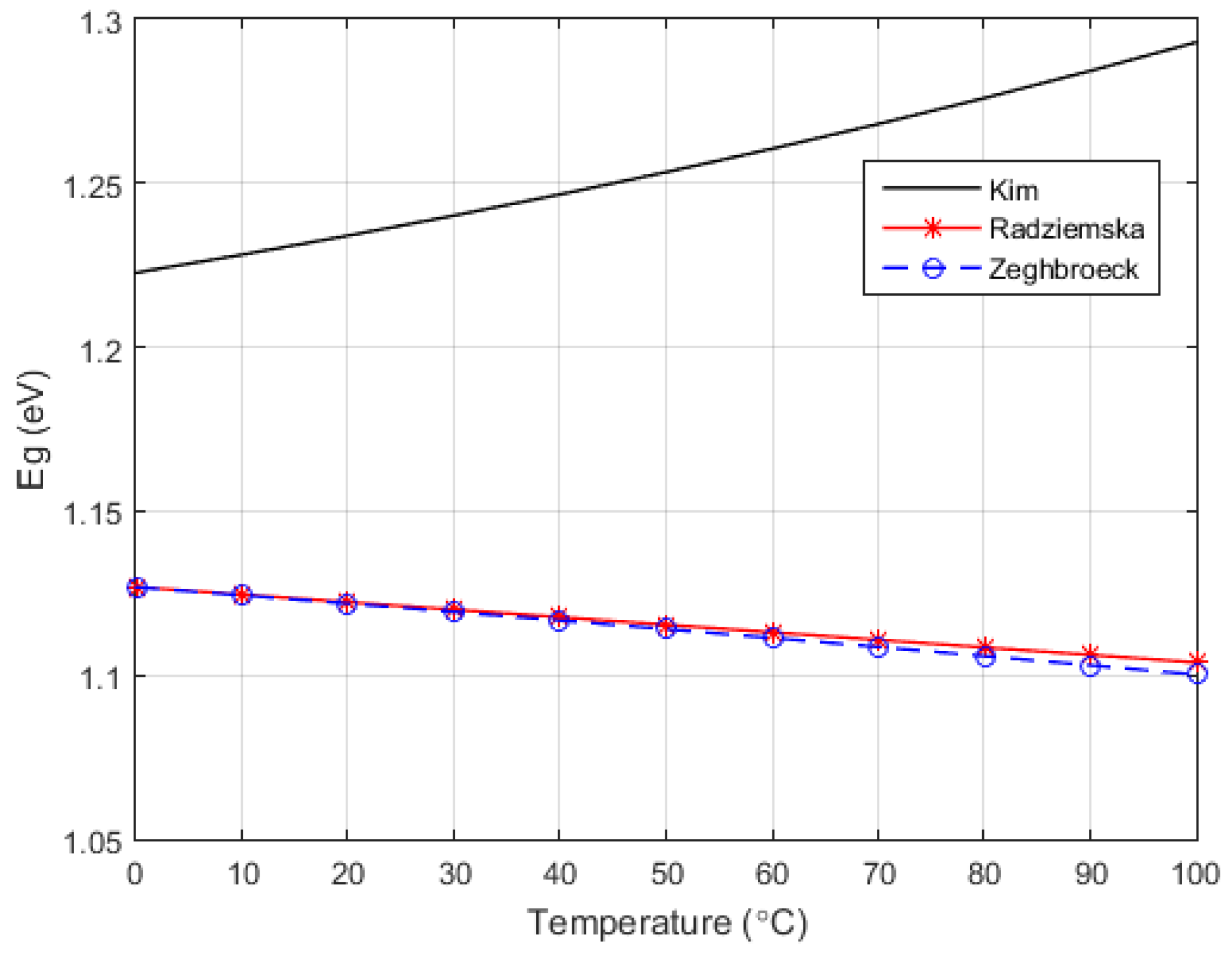
4.2.2. Band Gap Energy and Bandgap Voltage—
Van Zeghbroeck [
8] shows that the bandgap energy,
, exhibits a small temperature dependence as in (16).
From (16),
for silicon cells at 25 °C. This is the value considered in
Table 1.
In contrast, Kim et al. [
23] define the variance for
for silicon to be:
Both (16) and (17) fit in the [1.1, …, 1.3] V interval specified when Equation (12) was introduced. In our approach shown in
Figure 3, we adopted the Van Zeghbroeck proposal because it will finally lead to a more realistic value for
and close to the linear approximation of
against temperature suggested by Radziemska and Klugmann [
40], which indicate a temperature coefficient
.
4.2.3. Series Resistance—
Honsberg and Bowden [
7] show that
does not influence
, but close to the open-circuit voltage, the I-V curve is affected by
. An initial estimation for
is to find the slope of the I-V curve at the open-circuit voltage point (18):
In our case, mΩ (while mΩ, as it will later be shown).
Cuce and Bali [
43], Cuce et al. [
47] and Singh et al. [
42] claim that
linearly decreases with the temperature. Obviously, reducing
yields an increase in the output current.
A PV Cell model is also available in MATLAB Simscape [
52]. It consists of the same circuit as in
Figure 1, where the user can choose between:
Both models adjust the resistance values and current parameters as a function of temperature. Resistance
is assumed to be given by (19):
where
is the temperature exponent for
.
is 0 by default and when modified has to be positive.
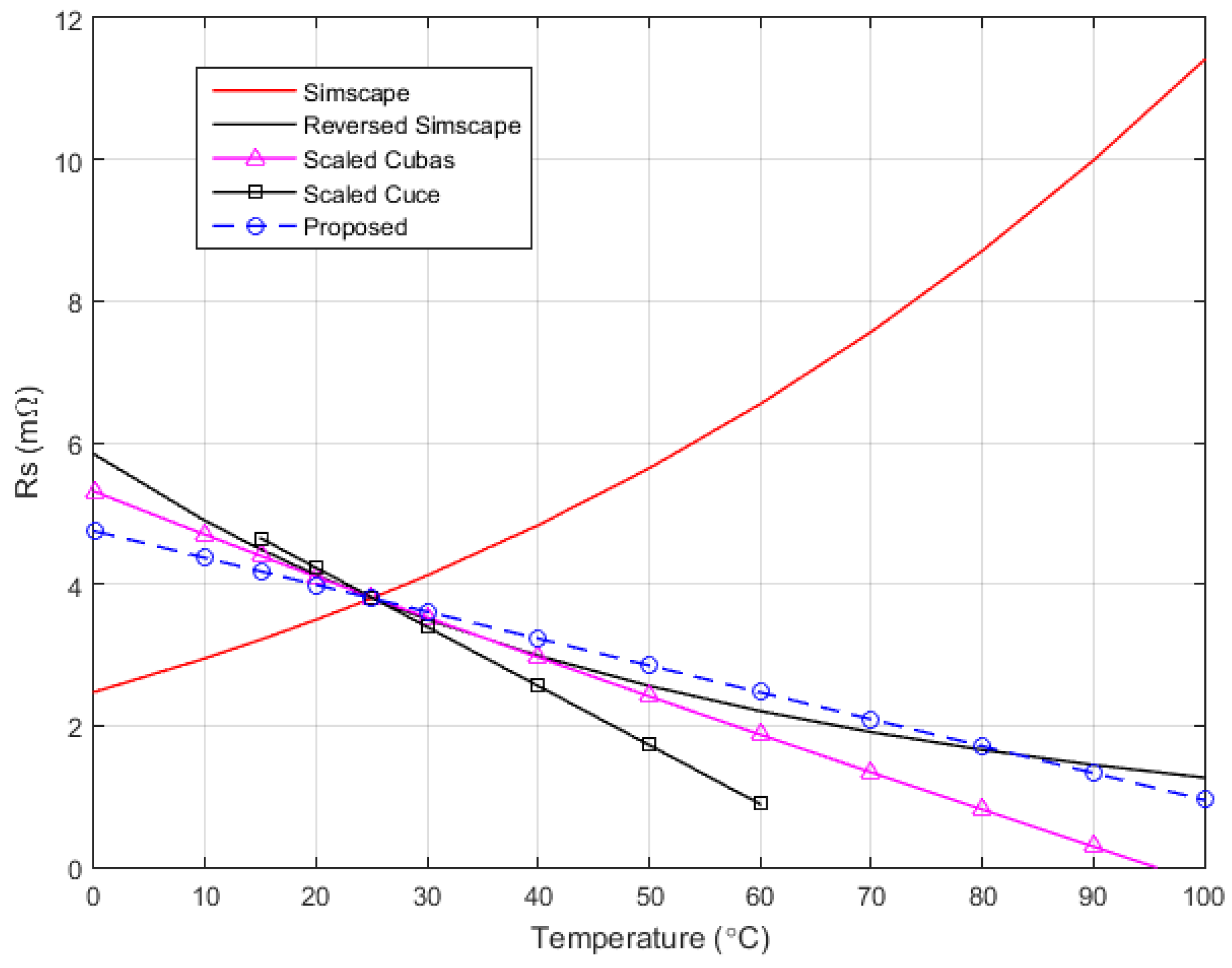
Figure 4 summarizes all these above dependencies. In order to have the results in the same range, Cubas et al. [
31] and Cuce et al. [
47] results were scaled, and Equation (19) was re-written as in (20), interchanging
with
and
was estimated as 4.9 for the best fit. A linear dependency is easy to implement, but might also lead to results not physically true (for example Cuce et al. [
47] data lead to negative
resistances for temperatures over 75 °C and so does Cubas et al. [
31] over 97 °C).
where
.
The linear law (21) was adopted for
and we chose
, again for the best fit.
4.2.4. Parallel Resistance—
Honsberg and Bowden [
7] and Jung and Ahmed [
25] showed that the shunt resistance of a solar cell can be determined from the slope of the I-V curve close to the short-circuit point, yielding a fair approximation for
:
From our experimental data, Ω, very close to the accurate solution Ω, as it will later be illustrated.
Cuce and Bali [
43] and Cuce et al. [
47] claim that the shunt resistance linearly decreases with temperature. They explain this decrease in terms of a combination of tunneling and trapping–detrapping of the carriers through the defect states in the space-charge region of the device. These defect states act either as recombination centers or as traps depending upon the relative capture cross sections of the electrons and holes for the defect. Temperature dependency for
is however more complicate.
is again modeled in MATLAB Simscape like (23):
where
is the temperature exponent for
.
is 0 by default and when modified has to be positive.
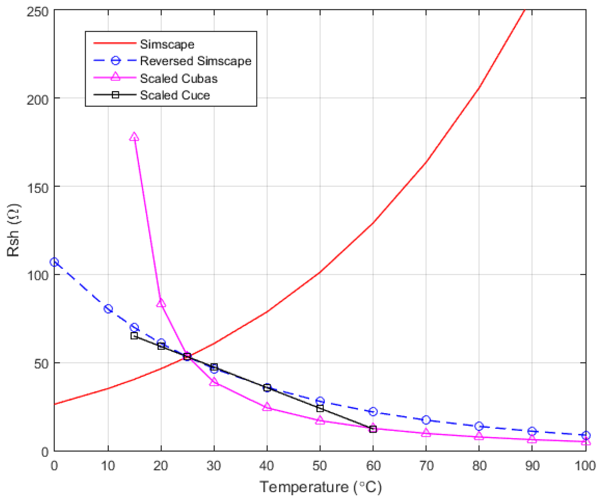
Figure 5 summarizes all these
equations. In order to bring the results in the same range, Cubas et al. [
31] and Cuce et al. [
47] dependencies were scaled, and Equation (23) was re-written as in (24) interchanging
with
and
was estimated as 8 for best fit.
where
.
Although influence is small in the overall model, for an accurate modeling and especially for larger temperature ranges linear variation is not realistic. Therefore in our model described by (24) we chose .
4.2.5. Ideality Diode Factor—
Some authors consider the ideality factor as being constant over the operating temperature range and with a generic value for
in the interval [1, 1.5] for every kind of cell [
22,
31]. Cuce et al. [
29] propose
for monocrystalline silicon cells, and
for polycrystalline ones. Some studies indicate a linear decreasing with temperature [
18]. Cubas et al. [
31] say that “the lack of accuracy produced when considering the ideality factor as constant is generally reduced, given that variations of this parameter only affects the curvature of the I-V curve.” This is arguable, as
interferes in an exponential dependency and small variations of
lead to significant changes in
and finally in
. One might say that picking a random
in the above specified range will be balanced by a different
, so only the pair
matters. However this approach is misleading, as it may induce impossible physical solutions.
Phang et al. [
13] have the following proposal:
De Blas et al. [
17] suggest that:
E. Saloux et al. [
28] somehow simplify (26) as below:
In the algorithm of Villalva [
53], a different formula is introduced. Considering that for crystalline silicon
J,
becomes 1.1235 V and the following formula provides a good result (Formula (28) was adapted from [
53], as the additional presence of the
in the initial formula provided correct results only for
), thus eliminating a trial and error time consuming for the initial guess of
:
The results for
are summarized in
Table 3, with a very good correlation between (25), (26) and (28). This is the reason we have adopted the Villalva value of 1.2034.
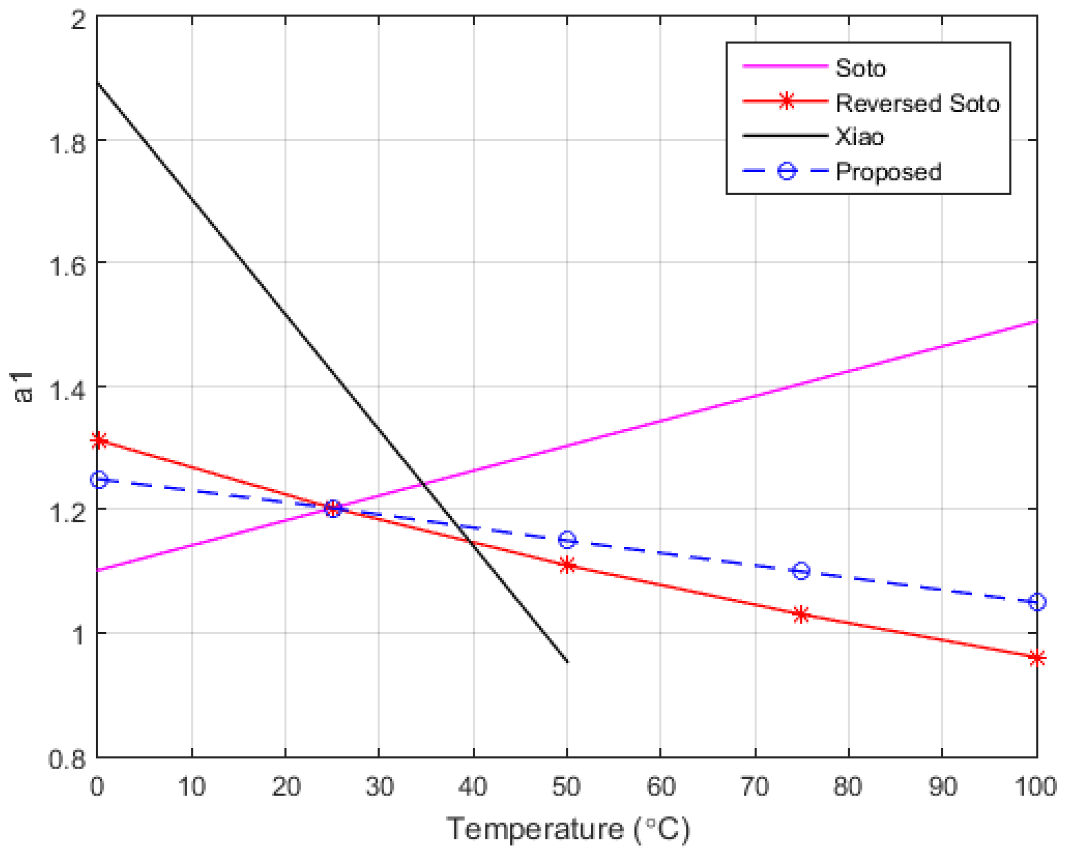
Xiao et al. [
18] specify a linear decreases of the ideality factor with the temperature for the Shell ST40 module, ranging from 1.85 to 1.15, corresponding to 5 to 45 Celsius degree variance respectively. From the data plotted in their work, the following law can be adopted:
Such approach must be taken with extreme care, as it is a common practice to operate often at temperatures higher than 48 °C, where (29) yields (or 0 at 100 °C)
De Soto et al. [
20] come with a different proposal:
which has a wrong slope. For a proper variation
and
should be reversed as follows:
Our experiments presented in
Figure 6 yielded a different result, closer to reversed Soto (31), according to the following linear dependency:
4.2.6. Self Heating Phenomenon
It is a common practice to express the internal cell temperature,
based on Normal Operating Cell Temperature (NOCT) data, when the module is mounted 45° from horizontal.
Here
W/m
2,
°C and airflow is
m/s [
45].
The internal temperature of the PV was of permanent concern for the researchers [
40,
41,
42,
46], but in most situations just an uncorrelated dependency is studied. Simply the temperature dependency of the I-V characteristic without acknowledging neither the real, actual temperature of the PV nor parameter variation is considered. Advanced simulators software packages include such features, MATLAB Simscape [
52] being one of them.
In a recent work, Krac and Górecki [
54] introduced a thermal model for the PV cell, where the self heating is modeled. The thermal behavior is modeled by a thermal resistor and a thermal capacitor, a voltage source related to the ambient temperature and a current source that represents the total dissipated power within the PV. They claim that “for the maximum allowable value of the panel forward current (equal to 8 A), a self heating phenomenon causes an increase in the panel temperature value equal only by 12 °C.” In our experiments, we acquired a rather extended influence, ranging from 20 to 30 °C.
Opposite to [
55,
56], the power dissipated by the PV cell is taken into account from the dissipative elements, which are resistive in our model. The energy flows from the two current sources to the resistors and the external circuit. Two or three current sources (or even diodes) are used in order to model different phenomena that take place inside the PV cell, the photoelectric effect and the behavior of p-n junction [
8].
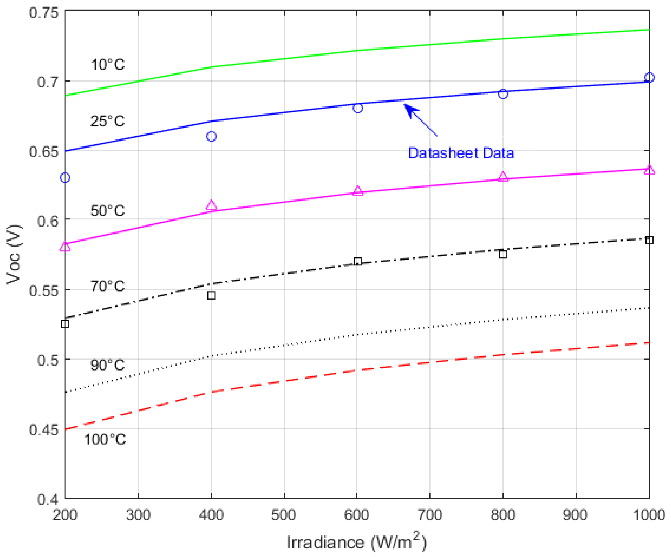
4.2.7. Open Circuit Voltage—
Ishaque and Salam [
27] propose for the
the following variation (34), which proves good correlation with the datasheet info and experimental data—see also
Figure 7:
Even (34) is not necessary for the model, it is another starting point for computing .
4.3. The New Proposed PV Cell Model
The proposed model is presented in
Figure 8. The upper section consists of standard elements, while the thermal modeling is ensured by the lower section. Here the current source labeled
simulates the power dissipated in the cell, the voltage labeled
is the cell temperature and the air temperature is modeled by the voltage source
. The thermal resistance
models the thermal flow through the system structure, in our case the PV cell. The thermal capacitance
models the thermal inertia of the PV cell. Both
and
emulate all thermal transmission phenomena (conduction, convection and radiation) and depend of the materials, the finishing of the surfaces and on the mechanical dimensions of the system.
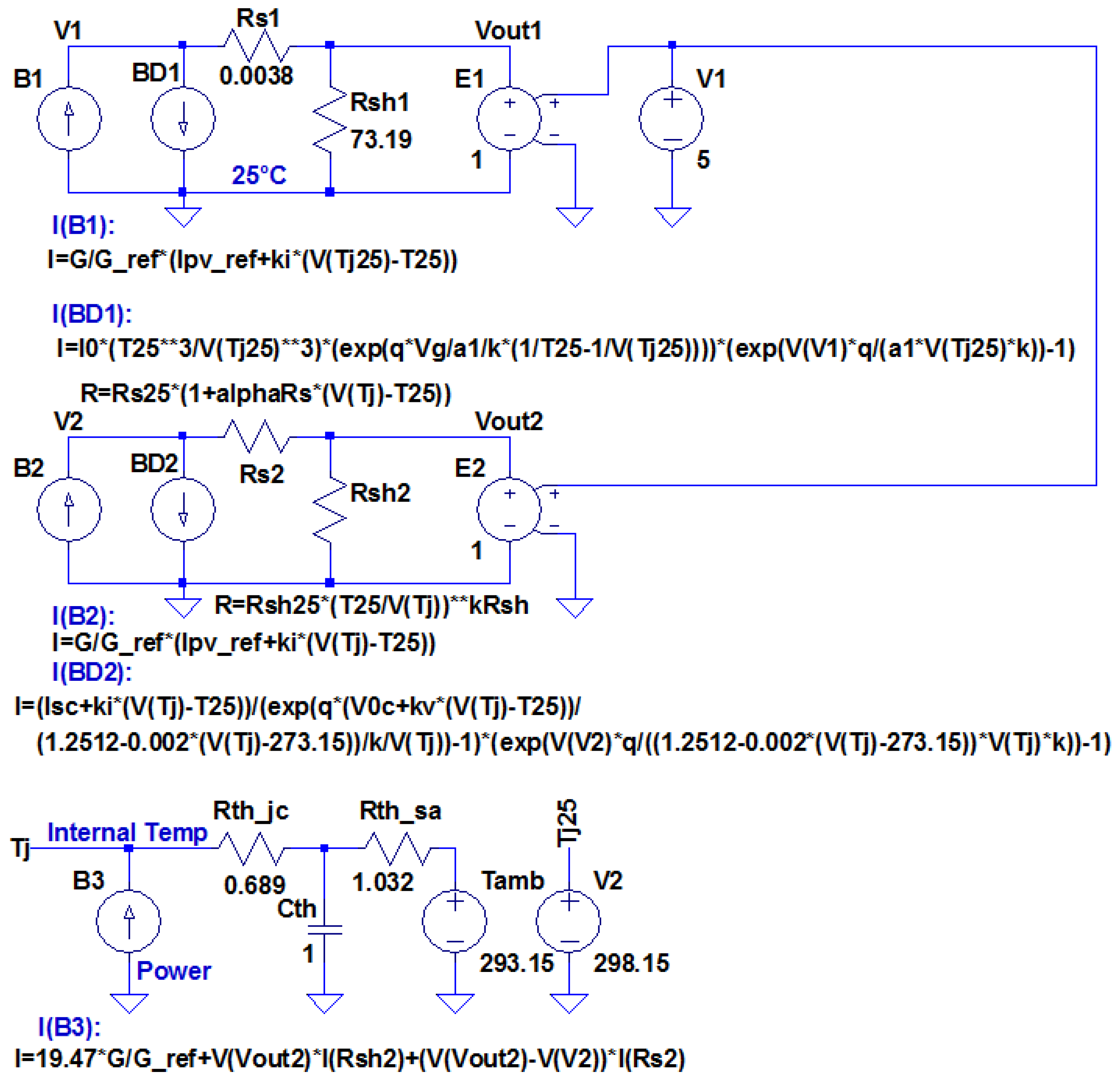
The practical LTSpice model implementation is depicted in
Figure 9 and can be found at
http://tess.upt.ro. The upper circuit addresses the standard conditions (for reference and validation), while the middle section deals with the thermal model of the PV solar cell. The power associated with the circuit also includes the power due to the irradiance scaled with the cell area and the electrical power dissipated in
and
.
The thermal parameters
and
were extracted from experimental data, similar to [
54]. After a set of data was acquired, the temperature against time curve variation was fit and the time constant and the steady state value were determined. Unlike Górecki and Krac [
55,
56], we considered no dissipated power occurs in the BD2 current source of the model in
Figure 9, as it makes no physical sense.
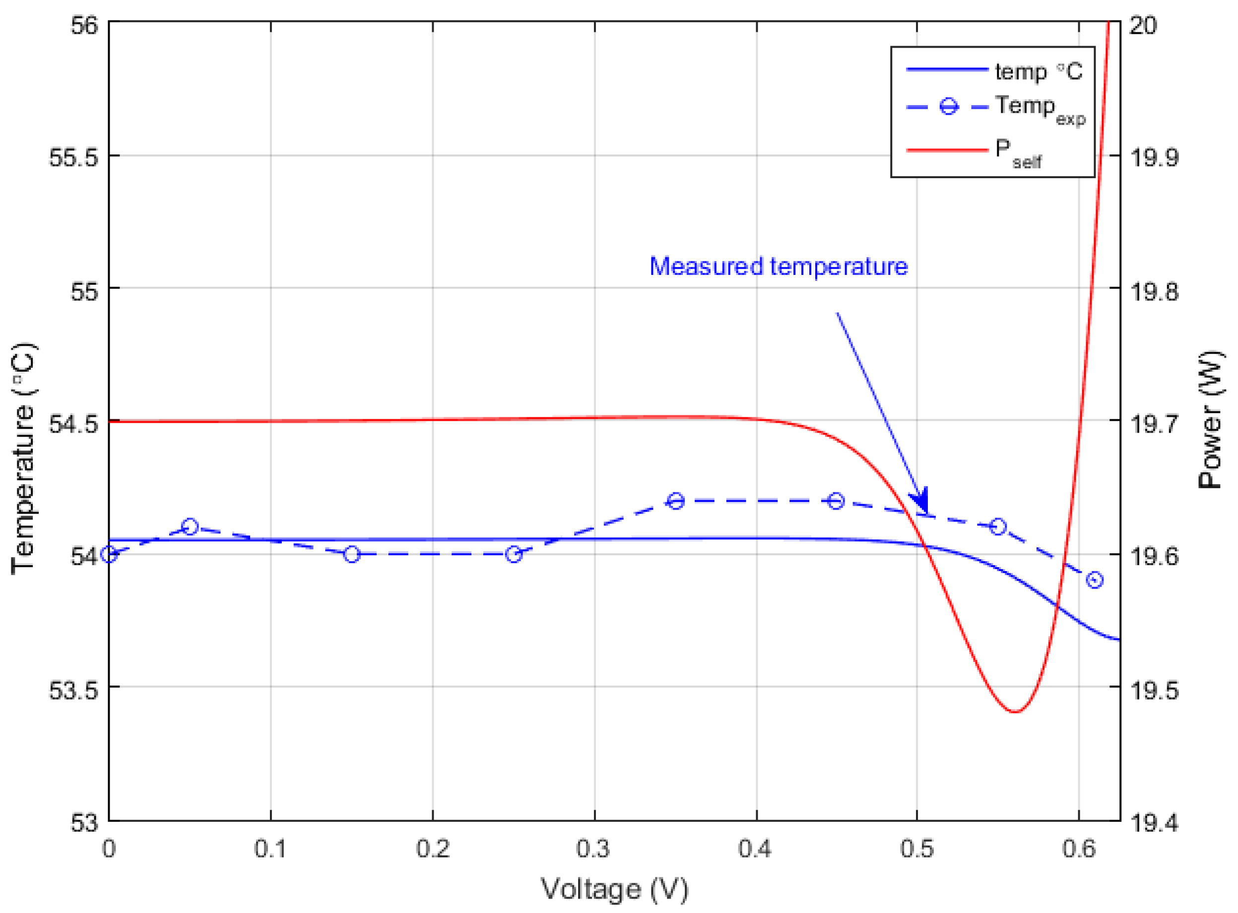
5. Experimental Results
Figure 10 exhibits the simulated and the measured internal temperature of the PV cell and the dissipated power variation. It is worth mentioning that the corresponding NOCT for the temperature in
Figure 9 is 47.2 °C.
Table 4 summarizes the main results for both the proposed model and the experiments performed for the PV cell. It can be observed that perfect agreement between the simulated and measured results is achieved.
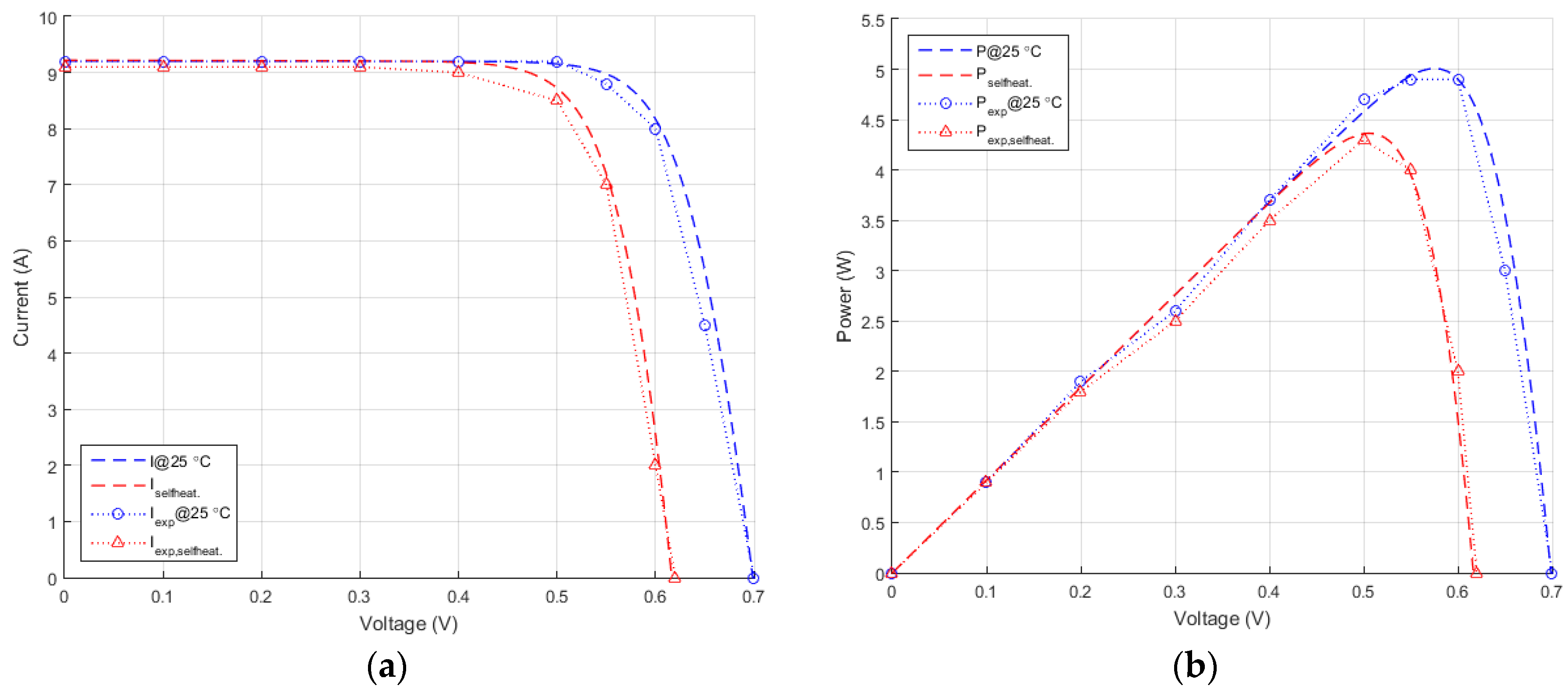
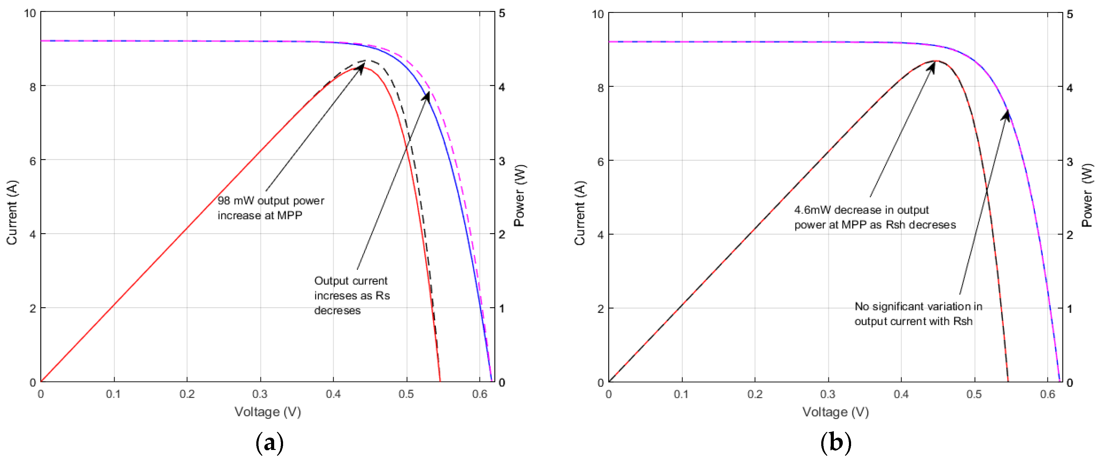
The final validation of the model is presented in
Figure 11 and
Figure 12. Here the I-V and P-V characteristics of the PV cell are plotted at the reference temperature and at the operating temperature. Experimental data is represented with markers while the lines correspond to simulated results with the model proposed. A good correlation between the model and the experiments can be noticed.
Figure 12a displays the serial resistance
influence on the output current and power. The solid lines graphs correspond to a fixed
while the dashed lines correspond to variable
with all the parameters included. At MPP a 98 mW power increase was observed. As estimated before,
has a minor influence on the PV output—only 4.6 mW power decrease at MPP could be noticed, as displayed in
Figure 12b. It is worth mentioning that in all cases the model self-computes the appropriate values for
and
based on the predicted internal temperature.
PV arrays compared (
Table 5) were monocrystalline (Shell SP-70, MSMD290AS-36.EU and multycrystaline (Kyocera KG200GT, MSP300AS-36.EU, MSP290AS-36.EU, Sharp ND-224uC1).
All the data from
Table 5 was processed with the above proposed algorithm and the results are listed in
Table 6, along with similar results from other researchers.
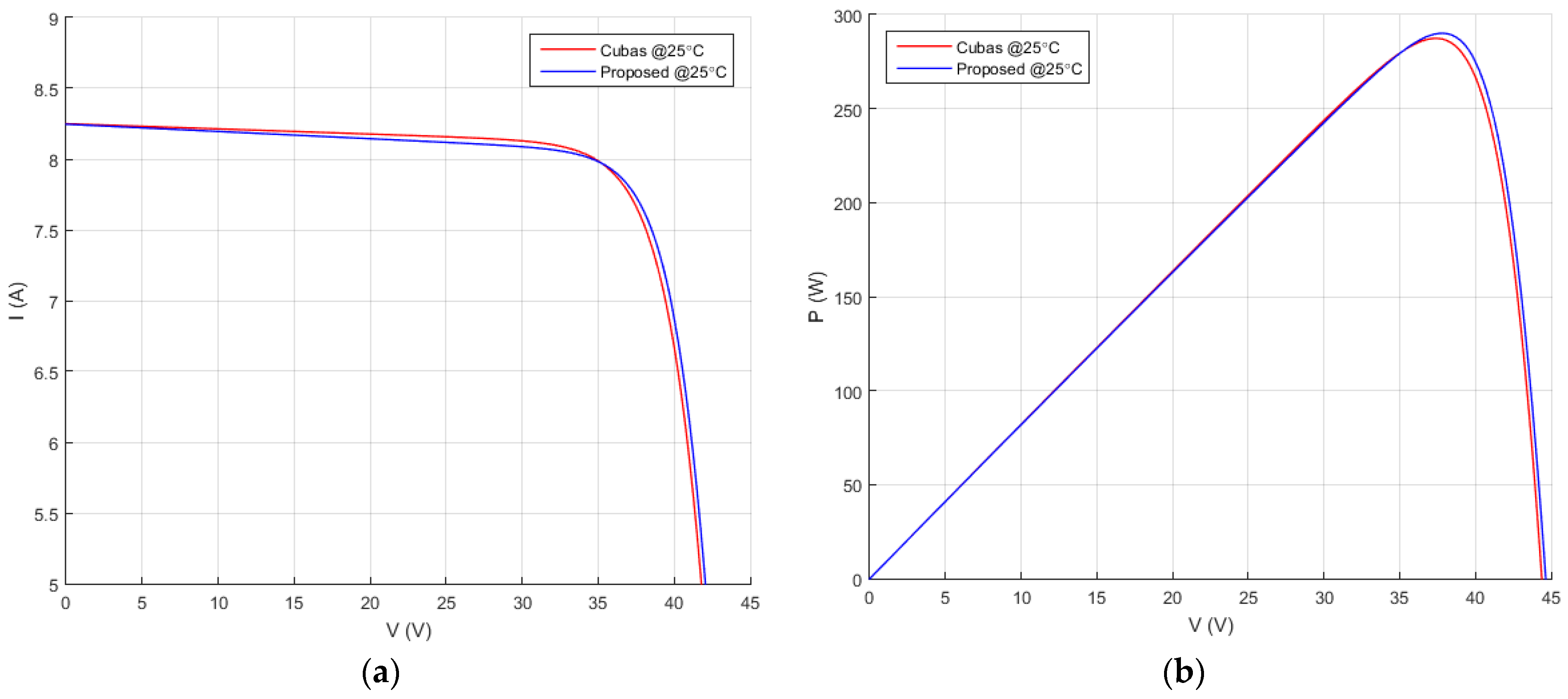
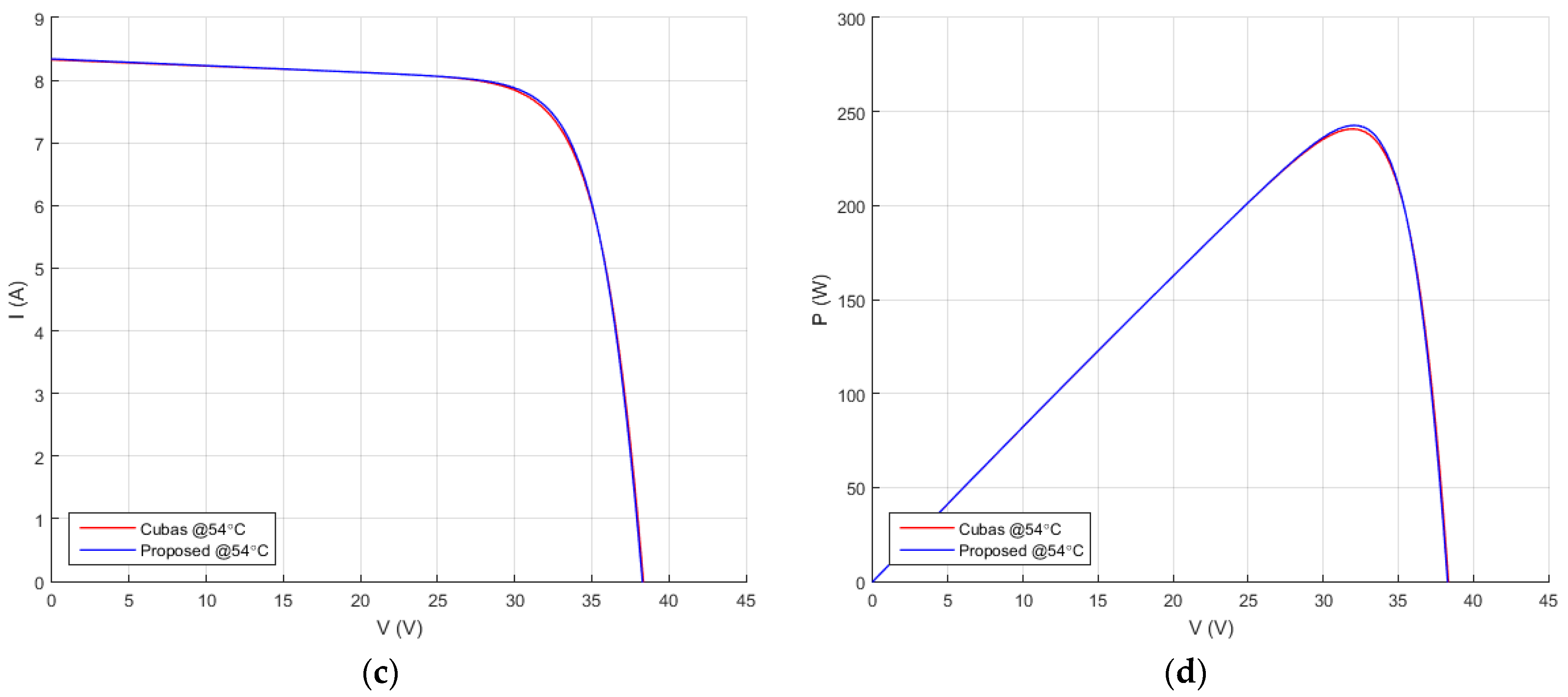
The final validation of the model was by applying the introduced model and computation method for the MSMD290AS-36.EU monocrystalline PV cell array and compare the results to the ones provided by Cubas et al. [
31], as shown in
Figure 13. As it can be seen, a good correlation exists between the two approaches.
6. Conclusions
A new thermo-electrical model for the PV cell was introduced. Only free available tools were used during modeling. The literature analysis proved discrepancies between authors when studying parameters variation and a more precise model is proposed in this paper.
The model proved to be accurate, while considering parameter variation and selfheating phenomenon. To the best of our knowledge this is the first time when all these parameters are included in a PV model. The internal silicon operating temperature at 1 Sun (with the ambient temperature being 20 °C) is 54 °C predicted by our model and validated by measurements performed with the FLIR and the PT1000 sensors.
As other authors have mentioned, influence is relatively reduced in the model. However proved to be a major factor. displayed a small variance with temperature. Resistance influence is important but sometimes shadowed by the wiring. The proposed model was accurately confirmed and validated by the experiments.


