Comparative Modeling of a Parabolic Trough Collectors Solar Power Plant with MARS Models
by
Jose Ramón Rogada
1, 
Lourdes A. Barcia
2,
Juan Angel Martinez
3,
Mario Menendez
1 and
Francisco Javier De Cos Juez
1,* 1
Department of Exploitation and Prospection of Mining, University of Oviedo, 33004 Asturias, Spain
2
NORMAGRUP TECHNOLOGY S.A. Llanera, 33420 Asturias, Spain
3
Department of Electrical Engineering, University of Oviedo, 33004 Asturias, Spain
*
Author to whom correspondence should be addressed.
Energies 2018, 11(1), 37; https://doi.org/10.3390/en11010037
Submission received: 3 October 2017
/
Revised: 18 December 2017
/
Accepted: 19 December 2017
/
Published: 25 December 2017
Abstract
:Power plants producing energy through solar fields use a heat transfer fluid that lends itself to be influenced and changed by different variables. In solar power plants, a heat transfer fluid (HTF) is used to transfer the thermal energy of solar radiation through parabolic collectors to a water vapor Rankine cycle. In this way, a turbine is driven that produces electricity when coupled to an electric generator. These plants have a heat transfer system that converts the solar radiation into heat through a HTF, and transfers that thermal energy to the water vapor heat exchangers. The best possible performance in the Rankine cycle, and therefore in the thermal plant, is obtained when the HTF reaches its maximum temperature when leaving the solar field (SF). In addition, it is necessary that the HTF does not exceed its own maximum operating temperature, above which it degrades. The optimum temperature of the HTF is difficult to obtain, since the working conditions of the plant can change abruptly from moment to moment. Guaranteeing that this HTF operates at its optimal temperature to produce electricity through a Rankine cycle is a priority. The oil flowing through the solar field has the disadvantage of having a thermal limit. Therefore, this research focuses on trying to make sure that this fluid comes out of the solar field with the highest possible temperature. Modeling using data mining is revealed as an important tool for forecasting the performance of this kind of power plant. The purpose of this document is to provide a model that can be used to optimize the temperature control of the fluid without interfering with the normal operation of the plant. The results obtained with this model should be necessarily contrasted with those obtained in a real plant. Initially, we compare the PID (proportional–integral–derivative) models used in previous studies for the optimization of this type of plant with modeling using the multivariate adaptive regression splines (MARS) model.
1. Introduction
Nowadays, there is a social movement that is committed to the environment. This has resulted in a greater control over polluting emissions from industries that give us vital support (Kyoto 1992). The Kyoto protocol, which was a commitment to reduce pollution signed by more than 160 countries all over the world, has managed to reduce emissions by 22.6% in 10 years. Many actions have contributed to this achievement. Among them, the use of so-called alternative energy sources has played a relevant role.
One of the major renewable energy sources is the sun. Photovoltaic and solar thermal power plants have proliferated in recent years, and become a relatively mature [1] source of renewable energy. Nowadays, parabolic trough collectors (PTC) solar thermal power plants are the most technically developed, and therefore the most suitable, to test different controller models that assure an optimal behavior of the solar thermal plants, and improve the ones that are currently being used in them. Although studies have been developed in PTC power plants, all of the variables and properties of the materials (density, specific heat, and so on) have been introduced in the solar field (SF) model as parametric equations dependent on the temperature. By doing so, the methodology used to obtain the different controllers in a PTC power plant is very similar to that which would be used for other thermal power plants such as solar power towers, solar dish/engine systems, etc. Therefore, the results obtained with these types of controllers are expected to be very similar in any type of thermal power solar plant.
These PTC plants consist of different systems, as shown roughly in Figure 1:
- SF (solar field): Formed by the needed elements to collect solar radiation and transform it into thermal energy. The modeling [2] of diffuse solar radiation at different planes, as well as at ground level, already represents an exclusive field of study in modeling efficient power plants.
- TES (thermal energy storage): It contains all of the elements in charge of storing the thermal energy, which is provided when the Sun is not enough. Even when other materials were tested, molten salts present more advantages in terms of security and cost. In any case, some others are being researched. The development of ternary and even quaternary mixtures of different types of salts has been studied [3]. These mixtures give a HTF (heat transfer fluid) with better operational characteristics. The lower melting points of these mixtures reduce the cost of the process by not needing an external energy supply to keep the mixtures melted at night.The study [4] of new mixtures other than the usual molten salts used as TES, provide satisfactory results in regard to stability, fluidity, and thermal inertia. These investigations could lead, in the near future, to the replacement of the salts in the TES by these types of mixtures, and even the use of the same as HTFs.
- Gas Heater: It provides energy for either maintaining the HTF above its melting point at night or on a cloudy day, or helping the SF to increment the power that heats the fluid by using natural gas. This block is used when the molten salt block does not have enough energy to keep the fluid at an adequate temperature. In these cases, some additional energy must be spent in order to maintain the fluid in the liquid state until a new daily period of insolation begins.
- SG (Steam Generator). It is formed by a steam generator train which, thanks to the contribution of thermal energy, converts liquid water into steam. This steam drives a turbine connected to an electric generator that produces electricity.
In the case of the parabolic trough collectors (PTC) solar thermal power plants, the SF is compound by a set of mirrors placed in a parabolic-shaped structure. In the focus of the parabolic, several pipes are distributed along the mirrors. Inside the pipes, there is a HTF that circulates through the SF, absorbing thermal energy from the sun and transferring it to the TES and the SG, producing electricity.
Although other fluids have been analyzed to transfer the thermal energy (e.g., molten salts, water steam, water), and others are being researched (e.g., nanofluids and ionic fluids), most of the PTC power plants use a kind of synthetic oil for this.
As in all power plants, the main purpose is to produce as much as electricity as possible. In thermal plants, this objective implies generating the largest amount of steam. While this goal seems easy in conventional thermal plants, where the energy comes from fuel or gas, in solar plants where heating the fluid depends on an unpredictable energy source—the Sun—this is a major issue, since this source cannot be manipulated.
To produce as much steam as possible, it would be important to have the HTF working at its maximum operating point (around 400 °C). The synthetic oils should not exceed this point, since otherwise they would be degraded before expected.
Several ways to control the heating of the fluid can be found in the literature. Barcia et al. [5] described a model of a complete solar field. This model offers a graphic user interface that allows the user to relate the developed blocks with the different parts of a real HTF system. It is scalable, so it could be easily modified to model SFs of different sizes. Since the HTF properties have also been included in blocks, although the proposed model uses synthetic oil as its HTF, other alternatives could be included in a very easy way.
In Reference [6], a hybrid model is used. The study is based on data that do not have a common point or a certain response from the same assumption. It starts from the same assumption without a common response, but builds one that serves as an output to model the behavior.
All of them have the objective of the controller in common, which is to keep the fluid temperature at the output of the SF at its maximum level in spite of changes in the solar irradiation, wind, clouds, and so on. To get this objective, the parameter to be controlled is the HTF mass flow in such a way that if the fluid temperature tends to overcome the set point (maximum value), the controller causes the mass flow to increase in such a way that there is not enough time to heat it, and vice versa.
To test different strategies of control without interfering with the normal operation of the plants, models are used. In References [7,8,9], the authors use different algorithms based on artificial intelligence to study the interaction between variables. The advantage of these methods is that they can handle nonlinearities with relative ease, as long as they are based on an appropriate mathematical model.
For example, in Reference [10], a means of the chained equations method (MICE) was used to predict the solar radiation index. This is very useful for predictions with large change inertia in a few minutes, and where the most logical variables do not explain the main one, which is the temperature in this case.
In other cases [11], the different control strategies of this type of plant or similar are established based on the control of the different variables. It is easy to separate the variables that directly affect the process, study their fluctuations, and then develop control strategies according to the moment and the operating needs.
Analytical models [10] can offer a quick and accurate evaluation of the working sequences of this type of plant. The analytical nature of these models provides a picture that clearly explains the main dependencies of the different systems that make up these plants.
In References [5,12], the authors develop a model for the whole solar field with all of the mirrors, pipes, and loops of a real 50 MW PTC Solar Plant: La Africana, which is located in Córdoba (Spain). This plant has an installed capacity of 50 MW, and it is capable of producing 180 GWh per year, supplying energy to 100,000 homes. It has a thermal storage system (TES) providing seven hours of autonomy. The SF consists of 225,792 mirrors distributed in 168 loops. In spite of this model’s simplicity, it is accurate enough to test different controllers and compare them with the PID (proportional–integral–derivative), which is the controller mostly used in these plants. In Reference [13], the authors use this model to compare the PID controller with a PID with feed-forward (PIDFF) and an adaptive predictive expert (ADEX) control, concluding that both of them substantially improve the PID behavior overall when rapid changes in solar irradiation occur.
The objective of this work is to check the suitability of a type of control based on data mining to control the temperature at the output of the SF in such a way that the HTF is always working at its maximum operating point, no matter the value of the disturbances such as solar irradiation, wind velocity, and so on.
Since the fluid is very sensitive to changes in its temperature and should not exceed its maximum operating point, the control of the HTF heating process must be precise and fast. The use of intelligent models as multivariate adaptive regression splines (MARS), where no feedback loop is necessary, have shown a higher precision as well as a shorter answer time than the traditional PID based controllers. This makes these kinds of models very suitable for this application.
In Section 2 (Methods and Data), data mining over splines technology is explained, and how the MARS [6,8,10] algorithm could control the process of heating the HTF. This section also contains an explanation of the protocol that has been used to train the controller in order to get the most accurate results without the necessity of any feedback loop in the process. The system includes knowledge of its own experience. Section 3 (Results and Discussion) outlines the different MARS models that have been tested, as well as which ones were selected for comparison with the PID and PIDFF results obtained in Reference [12]. Finally, some conclusions can be found in Section 4 (Conclusions).
2. Methods and Data
2.1. Multivariate Adaptive Regression Splines Method (MARS)
The MARS model of a dependent variable with M basis functions [14,15,16], can be written as:
where is the dependent variable predicted by the MARS model, c0 is a constant, Bm(x) is the mathematical base function, which can be a simple spline base function, and cm is the coefficient of the mathematical base function.
The MARS technique builds its model in two stages, the “step forward” and the “step back” [17,18,19]. In reference to the “step forward”, MARS begins with a model containing only the intercept term, which is the mean of the response values.
At each step, it finds the pair of base functions that give the maximum reduction in the residual sum of squares error. These two base functions are identical, except on one side they’re different from a function of a mirrored hinge that is used for each function. Each new basis function consists of a term that is already used in the model, multiplied by a new hinge function. The hinge function is defined by a variable and a knot, which means that, in order to add a new function base, MARS must search all of the combinations in the following way:
- existing terms (called parent terms in this context),
- all of the variables (to select one of the new basis functions),
- all of the values of each variable (for the knot of the new hinge function).
This process of adding terms continues until the residual error difference is too small to continue, or until the maximum number of terms is reached. The maximum number of terms is specified by the user before starting the construction of the model.
The “step forward” usually builds a model “overfit”. This model has a good fit to the data used to build the model, but will not generalize well to new data. To build a model with better generalization ability, the “step back” pruning model should be used. It removes terms one by one, eliminating the least effective term at each step until the best submodel is found. Subsets of the model are compared using the GCV (generalized cross-validation) criterion described below. The “step back” approach has an advantage over the “step forward”: it can choose any term to remove at any time, while the “step forward” approach in each step can only see the following pair of terms in each step. The “step forward” approach adds terms in couples, but the “step back” approach normally discards one side of the couple, and some terms are not seen as couples in the final model.
To determine which base functions should be included in the model, MARS uses the GCV [16,20,21]. In this way, the GCV is the means of the square residual error divided by a value that depends on the complexity of the model. The criterion for the GCV is defined as follows [17,18]:
where C(M) is a complex penalty that increases with the number of base functions of the model defined by [8,10,14,17].
where M is the number of the base functions defined in Equation (1), and the parameter d is a penalty for each function included in the basic base model.
C(M) = (M + 1) + d · M
Therefore, the GCV formula penalizes the addition of knots through these penalty parameters. In this sense, the GCV formula adjusts the training into a raw residual sum of square gross (RSS), to take into account the flexibility of the model [16,20,21]. In our study, the parameter d in Equation (3) is equal to 2, and the maximum level of interaction of the spline’s basis function is restricted to 2.
The technique of non-regression is not the best for all situations. The guidelines below are intended to give an idea of the pros and cons of the MARS technique [15,16,17].
- MARS models are more flexible than linear regression models [10].
- MARS models are easy to understand and interpret [15].
- MARS models can handle continuous and categorical data. MARS tends to be better than recurring division for numeric data, because the hinge functions are more appropriate for numeric variables than the constant segmentation used by recurring division.
- MARS models often require little or no data preparation. The hinge functions automatically divide input data, so the effect of outliers is contained. In this sense, MARS is similar to the recurring division that also divides data into distinct regions, although using a different method.
- MARS, as well as the recurrent division, automatically select variables, which means that it includes important variables in the model and excludes those of minor importance. We should bear in mind, however, that the selection of variables is not a solved problem yet, and there is usually some arbitrariness in the selection, especially in the presence of collinearity and concurvity.
- MARS models tend to have a good bias–variance trade-off, and are suitable for handling large data banks [22].
- The models of MARS, as with any other non-parametric regression, cannot directly calculate parameter confidence intervals and other controls in the model (unlike linear regression models). Cross-validation and similar techniques should be used to validate the model instead.
- Sometimes, MARS models do not give as good results as other model types, but can be built much more quickly and are more interpretable. An interpretable model is one that makes the effect of each predictor clear.
- MARS models can make predictions more quickly. The prediction function simply has to evaluate the MARS model formula. This is a fast prediction if we make a comparison to making a prediction about a support vector machine (SVM) model for example, where every variable must be multiplied by the corresponding element of every support vector. This can be a slow process if there are many variables and many support vectors.
2.2. Set of Experimental Data
As stated in Section 1 (Introduction), the proposed MARS controller has been implemented in the model described in Reference [5]. In this document, a complete dynamic model of the solar field of a real PTC solar plant is developed. The publication includes the PID controller currently used in the HTF heating process in most PTC solar plants.
This model has been used to check and compare the behavior of the process to different disturbances and input variables when different controllers are used. Thus, in Reference [15], the current PID is compared with a PIDFF and also with an ADEX, concluding that the PID is not the most appropriate regulator when there are abrupt variations in solar radiation. Although with all of those controllers, the error between the real temperature of the solar field output and the set point is negligible (around 0.0025%), with PIDFF, the time to reach the stationary regime is reduced by 78%, compared with a reduction of around 60% with ADEX.
In order to get a MARS controller accurate enough to be used in the HTF heating process, it is important to train it with the highest number of scenarios possible.
The inputs in our control process will be the temperature of the fluid at the input of the solar field (THTFC), as well as possible disturbances that can affect our process: for example, wind speed (Ws), solar radiation (DNI), ambient temperature (Tamb), incidence angle (ϕ), and optical performance of the collectors (ηopt). All of these disturbances are measurable. The original data are organized in the following way (Table 1):
There are a number of variables that the initial study [5] considers as perturbations, but in our intelligent model, they will be input data that have an impact on the training of the process output.
The objective of this phase is the generation of a control model that would work in an automatic and continuous way. Later, with available daily data, this model will generate optimal flow values for different input variables and disturbances. Note here that the main advantage of this kind of controller is the absence of a feedback loop. If the MARS model has been obtained by including the input variables under many different conditions, the model adapts to other possible new situations by responding to them without needing to know what is in the output of the process.
During the training phase, a representative sample of the set of input values (Tamb, THTFC, and DNI) is provided, together with the ideal output values (THTFH) that the model should generate for these entries. Therefore, to obtain the MARS control model, it was necessary to train different models that tested combinations of input stimuli and their corresponding outputs. This contributed to improving the response of the MARS models thanks to the progressive improvement in the definition of the training set.
Thus, the response of each model is used in the next model as knowledge learned. Models are trained to enhance the range of training stimuli, which makes it easy to approach a progressive and iterative final model that adapts better to the set point temperature of the thermal fluid. It must be indicated that the set point for these data, according to the normal process of the existing solar plant, is 393 °C.
All of the simulations were based on the following methodology:
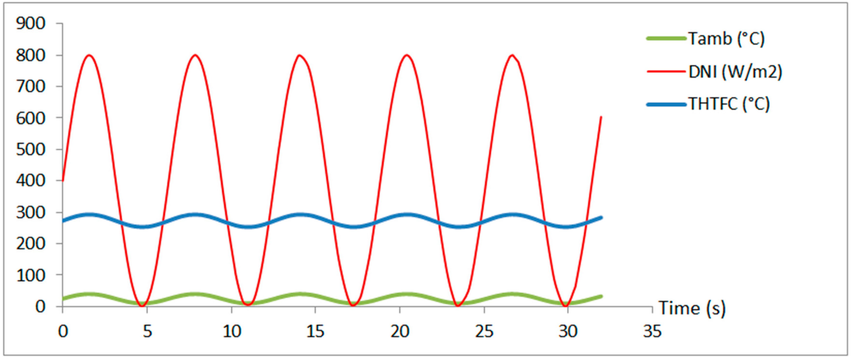
- Input values set definition. The input data set was obtained by combining artificially generated signals of sinusoidal, steps, and pulse type, with real measurements of the solar field. Figure 2 shows an example of how sinusoidal signals were generated.
In the same way, other input signals were generated to be used in the training of the model. Other real input signals taken from the La Africana PTC solar plant in different seasons and different years were also used to train the MARS controller. Figure 3 shows the input variables of the SF of the plant in September 2010:
- b.
- Training data set generation (DS_1). The input data set generated in step 1 was processed with the previously published tool [5], and the response of a feedforward PID controller to the above inputs was obtained: THTFC.
- c.
- Alternative training data set generation (DS_2). A second data set was defined from that obtained in step 2 by selecting only those inputs that generate outputs in the range of 390–396 °C, which is the ideal operating range of the plant.
- d.
- Training of the MARS model with the input data, obtained in the previous steps.
Figure 4 summarizes the process described above.
Finally, the results obtained with the MARS intelligent model are compared with those provided in the initial study, which were obtained through other algorithms such as the ones shown in Reference [15]: PIDFF and ADEX.
3. Results and Discussion
Different initial models were considered for obtaining the most accurate MARS controller. From DS_1, two models were selected (MARS_1a and MARS_1b). The initial model that came closest to the desired result was further developed. In this first approach, thermal inertia had not been taken into account. An ideal situation of the operations of the power plant was assumed.
The response of these models to disturbances in the input parameters was tested, and specifically, the response to an increase of the temperature of the HTF. In this stage, MARS_1b was considered to be the optimal model in terms of getting a THTFH close to the set point.
Due to the long distance that the fluid must travel from when it enters the SF until it leaves, the thermal power produced is delayed with respect to the received solar irradiation.
A variation of temperature at the inlet of the pipe is not seen at the exit until a certain time later. In the case of the solar field pipes, the transport delay is about half an hour for a nominal flow in a typical solar thermal of 50 MW and 168 loops.
If the flow was reduced by half, the transport delay would double. This means that there will be a delay in the thermal power supplied by the solar field with respect to the radiation received, which will be a function of the flow rate of the HTF circulating through it.
In a constant flow rate, an increase of radiation produces variation in the outlet temperature of the loop, which is approximately an increase with a delay with respect to the variation of irradiation.
However, in the collectors that join and mix the oil in the loops, the HTF of each loop has a different delay effect depending on the distance to the power block (power island), which is normally located in the center or north of the solar field. This is the main physical cause that will justify the disturbances in model results, which is explained in the next chapter.
The overall effect is that an increment of radiation translates not only into a delay but also into an added filter, which can be assimilated to an overdamped second-order response.
In a second stage, thermal inertia and mass flow were introduced to get more accurate models: MARS_2a and MARS_2b, respectively.
From DS_2, a fifth model (MARS_2c) was generated that took into account both oil thermal inertia and mass flow.
Table 2 shows a summary of the models that have been analyzed with differences between them:
Finally, these models were validated with real data from the operation of La Africana plant, on two different days.
3.1. First Responses
In the first place, responses of the different MARS models to a sharp change in the DNI (from 400 to 900 W/m2) were analyzed. Table 3 shows the results.
With the first model, called MARS_1a (Table 3), there is no overshoot. The mass flow follows the DNI variation perfectly. However, a short delay between the instant the signal changes and the system response was observed. Although this delay is lower than that in the PID system response [15], its occurrence must be found since the MARS model was trained taking into account the data obtained from the PID with feed-forward system Moreover, this model stabilizes at 393.5 °C, slightly above the set point 393 °C. It can also be seen that steady state is reached after 1100 s, well before when it is reached with PID (22,000 s) or PID with feed-forward control (5365 s) [15].
It was also observed that, for 400 W/m2 radiation, the temperature of 393 °C is never reached, but stays at approximately 387.5 °C, i.e., it is not correctly initialized.
With MARS_1b, although the value reached when the step occurs is closer to the set point, the value with which it is initialized is much lower.
The response of MARS_2a to the sharp step in DNI is better than the one with SIM models (MARS_1a and MARS_1b), in terms of reducing the time until the systems reacts to the step, as well as in the initializing, since the output is much closer to the set point.
The secondary model of this series, called MARS_2b, behaves similarly to the PID control with feed-forward with lower delay and establishment times, but with a slightly higher final temperature.
Regarding the third case, MARS_2c, although it stabilizes after the initialization to a lower value, it is closer to the set point in steady state.
This better behavior in the steady state of this MARS model compared with the former could be due to the “optimization” made in data collection.
Below is a summary of the behavior of different controllers versus the disturbance in the DNI. In this comparative (Table 4) overview, the following parameters have been taken into account:
- THTFpk: maximum temperature reached by the HTF of the SF when the DNI increases.
- Setting time: time elapsed from the beginning of the increase in the DNI to the moment when the temperature of the HTF of the SF reaches steady state.
- Error (%): percentage of error between the temperature of the HTF of the SF in steady state and the set point (established at 393 °C).
Looking at these results, it can be concluded that, although the methods based on PID controllers (PID and PIDFF) have a better response in terms of the error committed, when it comes to obtaining the shortest possible establishment time, the best option is MARS_2c [+Oil Thermal Inertia; +Mass Flow].
Table 5 defines the algorithm of MARS_2c [+Oil Thermal Inertia; +Mass Flow] model:
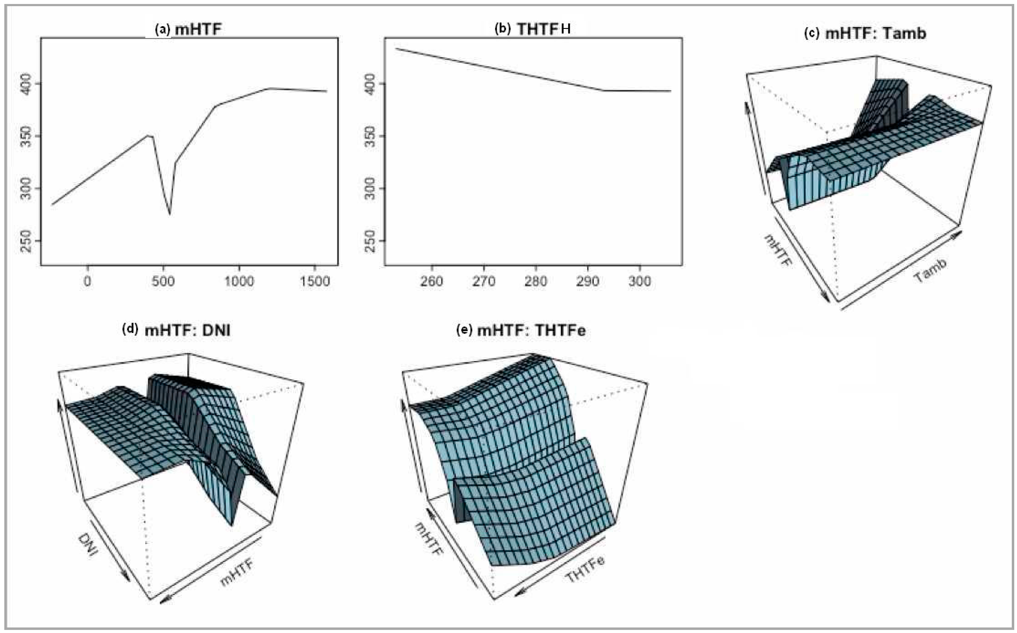
Figure 5 shows the graphics of the different terms that constitute the MARS model.
The main variables are reduced to only three: DNI, HTF mass flow, and input HTF temperature. The rest—ambient temperature, wind speed, and angle of incidence—are not considered a consequence of having less registers.
3.2. MARS Response to Real Input Data
After the research effort, the different models obtained were validated against the real data of the normal plant operation.
Figure 6 shows the different models’ responses as a function of the disturbances of the normal operation of the plant. These disturbances are related to the different and continuous conditions of daily plant operation, such as DNI, wind speed, the defocalization of collectors, and mass flow speed. In this case, real input variables taken on September 2010 in La Africana Solar Plant were used. The models that best follow the set point temperature with a lower setting time were MARS_2b [+Mass Flow] and MARS_2c [+Oil Thermal Inertia; +Mass Flow]. MARS_1b (Initial Data) took longer to reach set point. The reason for the better performance of these second models is that they are an evolution of the first one, with added conditions of control.
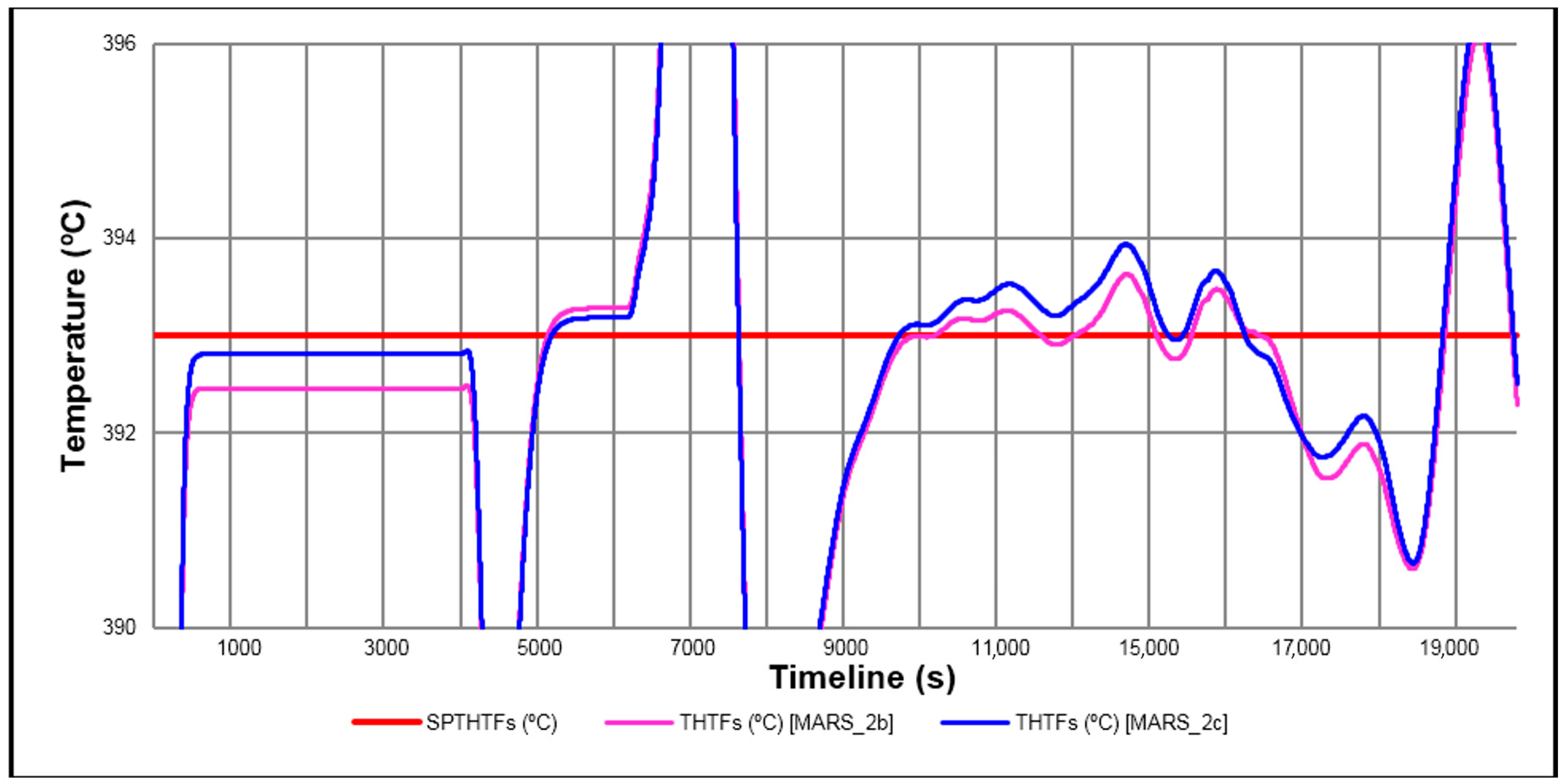
Another set of input variables was tested with just the best MARS models: MARS_2b [+Mass Flow] and MARS_2c [+Oil Thermal Inertia; +Mass Flow]. This time, data were taken from the real figures of La Africana in April 2011. The results of the responses can be seen in Figure 7.
In this case, models MARS_2b [+Mass Flow] and MARS_2c [+Oil Thermal Inertia; +Mass Flow] behave in a similar way, although model MARS_2c [+Oil Thermal Inertia; +Mass Flow] provided initial values closer to the set point, with a lower time of initial stabilization.
Table 6 shows the comparison between the different controllers’ responses to the data from April 2011.
4. Conclusions
The main conclusion is that it is possible to model the control process associated with the heating of the heat transfer fluid through MARS models and data mining techniques.
- Validation of the developed models has been conducted by using real data extracted from the SF, of La Africana, located in Cordoba. The fact that the MARS models respond appropriately to real data confirms the feasibility of this type of model in applications such as the one described.
- When suitably trained, MARS models’ initialization times are around 80% shorter than those obtained with conventional control strategies, which is because MARS control systems are operating in real time and through an open loop, without feedback.
- The settling time after variations in an input is up to 94% shorter than the one achieved with the PID control, and 73% shorter than that obtained with the PIDFF.
- Suitably trained MARS models present a response to variations of the DNI with smaller oscillations than those obtained with PID, and similar to those obtained with the PIDFF.
- It is necessary to take into account in the actual process the inclusion of oil thermal inertia effect through the solar field and the headers when the MARS models are being trained. Any future modeling for direct application must be based on actual data from each thermosolar plant exclusively.
- Input data collection for future modeling shall be expanded with data that follow all the points of the process in real time. We can consider that the input data are not representative of the direct training of a MARS model. We have made use of feedback and training already obtained from the actual PID control of the plant, as a complement to the proposed MARS models.
That the model based on splines can be represented as the sum of several simple polynomials of order two facilitates its implementation in any kind of architecture.
The results obtained demonstrate that data mining techniques are very suitable to model controllers for the heating of the HTF in thermal power solar plants. These types of controllers rise to an important reduction of the response time, which makes them faster than their PID counterparts.
It must also be pointed out that this is the first time that a data-mining-based controller is used in the HTF process of thermal solar plants, with the main advantage of the absence of any type of feedback loop. This largely simplifies the control of the plant, as well as makes it independent of possible sensor failure. Simultaneously, the lack of a feedback loop opens a whole field of study related to the evaluation of the performance of such control techniques.
Although in this case one type of intelligence-based technology has been proven to be suitable and effective, this work sets the basis for the application and evaluation of other intelligent algorithms.
Acknowledgments
The authors appreciate support from the Spanish Economics and Competitiveness Ministry, through grant AYA2014-57648-P and the Government of the Principality of Asturias (Consejería de Economía y Empleo), through grant FC-15-GRUPIN14-017.
Author Contributions
This paper will be part of the Ph.D. Thesis of Jose Ramón Rogada, who has therefore carried out most of the studies presented here. Francisco Javier de Cos Juez who was the supervisor of this study, and Lourdes A. Barcia, Juan Angel Martinez and Mario Menendez who had a relevant contribution, with their extensive previous studies of modeling through classic control systems.
Conflicts of Interest
The authors declare no conflicts of interest.
Glossary
| PTC | Parabolic Trough Collector |
| TES | Thermal Energy Storage |
| HTF | Heat Transfer Fluid |
| SF | Solar Field |
| SG | Steam Generator |
| PDI | Proportional Integral Derivative |
| PIDFF | PDI with Feedforward |
| MARS | Multivariate Adaptive Regression Splines |
| GCV | Generalized Cross Validation |
| SVM | Support Vector Machine |
| THTFC | HTF Cold Temperature in the solar field |
| THTFH | HTF Hot Temperature in the solar field |
| THTFpk | Maximum HTF Hot Temperature in the solar field |
| mHTF | HTF Mass Flow |
| WS | Wind Speed |
| DNI | Direct Normal Irradiance |
| Tamb | Ambient Temperature |
| ϕ | DNI incident angle |
| ηopt | Optical performance of the collectors |
References
- Thomas, A. Solar Steam Generating Systems Using Parabolic Trough Concentrators. Energy Convers. 1995, 37, 215–245. [Google Scholar] [CrossRef]
- Paulescu, E.; Blaga, R. Regression models for hourly diffuse solar radiation. Sol. Energy 2016, 125, 111–124. [Google Scholar] [CrossRef]
- Nunes, V.M.B.; Queirós, C.S.; Lourenço, M.J.V.; Santos, F.J.V.; de Castro, C.N. Molten salts as engineering fluids—A review Part I. Molten alkali nitrates. Appl. Energy 2016, 183, 603–611. [Google Scholar] [CrossRef]
- Wang, Z.; Wang, H.; Yang, M.; Sun, W.; Yin, G.; Zhang, Q.; Ren, Z. Thermal reliability of Al-Si eutectic alloy for thermal energy storage. Mater. Res. Bull. 2017, 95, 300–306. [Google Scholar] [CrossRef]
- Barcia, L.A.; Peón Menéndez, R.; Martínez Esteban, J.Á.; José Prieto, M.A.; Martín Ramos, J.A.; de Cos Juez, F.J.; Nevado Reviriego, A. Dynamic Modeling of the Solar Field in Parabolic Trough Solar Power Plants. Energies 2015, 8, 13361–13377. [Google Scholar] [CrossRef]
- Alvarez, J.; Guzmán, J.; Yebra, L.; Berenguel, M. Hybrid modeling of central receiver solar power plants. Simul. Model. Pract. Theory 2008, 17, 664–679. [Google Scholar] [CrossRef]
- Fernández, J.A.; Muñiz, C.D.; Nieto, P.G.; de Cos Juez, F.J.; Lasheras, F.S.; Roqueñí, M.N. Forecasting the cyanotoxins presence in fresh waters: A new model based on genetic algorithms combined with the MARS technique. Ecol. Eng. 2013, 53, 68–78. [Google Scholar] [CrossRef]
- De Andrés, J.; Sánchez-Lasheras, F.; Lorca, P.; Juez, F.J.D.C. A hybrid device of self organizing maps (SOM) and multivariate adaptative regression splines (MARS) for the forecasting of firms’ bankruptcy. Account. Manag. Inf. Syst. 2011, 10, 351–371. [Google Scholar]
- De Cos Juez, F.J.; Lasheras, F.S.; Nieto, P.G.; Álvarez-Arenal, A. Non-linear numerical analysis of a double-threaded titanium alloy dental implant by FEM. Appl. Math. Comput. 2008, 206, 952–967. [Google Scholar] [CrossRef]
- Turrado, C.C.; López, M.D.C.M.; Lasheras, F.S.; Gómez, B.A.R.; Rollé, J.L.C.; Juez, F.J.D.C. Missing data imputation of solar radiation data under different atmospheric conditions. Sensors 2014, 14, 20382–20399. [Google Scholar] [CrossRef] [PubMed]
- Salazar, G.A.; Fraidenraich, N.; de Oliveira, C.A.A.; de Castro Vilela, O.; Hongn, M.; Gordon, J.M. Analytic modeling of parabolic trough solar thermal power plants. Energy 2017, 138, 1148–1156. [Google Scholar] [CrossRef]
- Barcia, L.A.; Peon, R.; Díaz, J.; Pernía, A.M.; Martínez, J.Á. Heat Transfer Fluid Temperature Control in a Thermoelectric Solar Power Plant. Energies 2017, 10, 1078. [Google Scholar] [CrossRef]
- Baccioli, A.; Antonelli, M. Control variables and strategies for the optimization of a WHR ORC system. In Proceedings of the IV International Seminar on ORC Power Systems (ORC 2017), Milano, Italy, 13–15 September 2017. [Google Scholar]
- Friedman, J.H.; Roosen, C.B. An introduction to multivariate adaptive regression splines. Stat. Methods Med. Res. 1995, 4, 197–217. [Google Scholar] [CrossRef] [PubMed]
- Friedman, J.H. Multivariate Adaptive Regression Splines. Ann. Stat. 1991, 19, 1–67. [Google Scholar] [CrossRef]
- De Cos Juez, F.J.; Sanchez Lasheras, F.; Roqueñi, M.N.; Osborn, J. An ANN-based smart tomographic reconstructor in a dynamic environment. Sensors 2010, 12, 8895–8911. [Google Scholar] [CrossRef] [PubMed]
- Suarez Sanchez, A.; Iglesias-Rodriguez, F.J.; Riesgo Fernandez, P.; De Cos Juez, F.J. Applying the K-nearest neighbor technique to the classification of workers according to their risk of suffering musculoskeletal disorders. Int. J. Ind. Ergon. 2016, 52, 92–99. [Google Scholar] [CrossRef]
- Suárez Sánchez, A.; Krzemień, A.; Riesgo Fernández, P.; Iglesias Rodríguez, F.J.; Sánchez Lasheras, F.; de Cos Juez, F.J. Investment in new tungsten mining projects. Resour. Policy 2015, 46, 177–190. [Google Scholar] [CrossRef]
- Casteleiro-Roca, J.L.; Calvo-Rolle, J.L.; Méndez Pérez, J.A.; Roqueñí Gutiérrez, M.N.; de Cos Juez, F.J. Hybrid Intelligent System to Perform Fault Detection on BIS Sensor during Surgeries. Sensors 2017, 17, 179. [Google Scholar] [CrossRef] [PubMed]
- De Cos Juez, F.J.; Lasheras, F.S.; García Nieto, P.J.; Suárez, M.S. A new data mining methodology applied to the modelling of the influence of diet and lifestyle on the value of bone mineral density in post-menopausal women. Int. J. Comput. Math. 2009, 86, 1878–1887. [Google Scholar] [CrossRef]
- Vapnik, V. Statistical Learning Theory; Wiley-Interscience: New York, NY, USA, 1998. [Google Scholar]
- Galán, C.O.; Lasheras, F.S.; de Cos Juez, F.J.; Sánchez, A.B. Missing data imputation of questionnaires by means of genetic algorithms with different fitness functions. J. Comput. Appl. Math. 2017, 311, 704–717. [Google Scholar] [CrossRef]
Figure 1.
Schematic figure of energy production in a solar field power plant [5].
Figure 1.
Schematic figure of energy production in a solar field power plant [5].
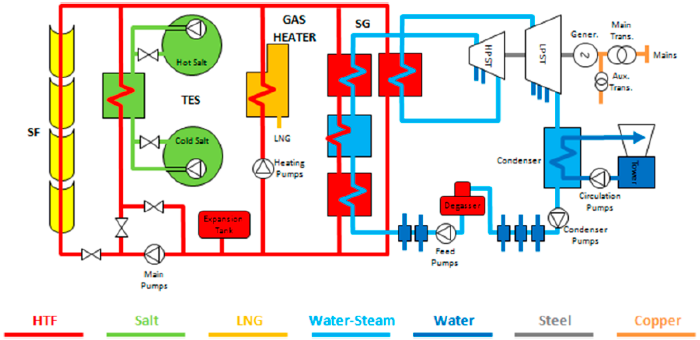
Figure 2.
Sinusoidal input variables.

Figure 3.
Real input variables (La Africana—September 2010).
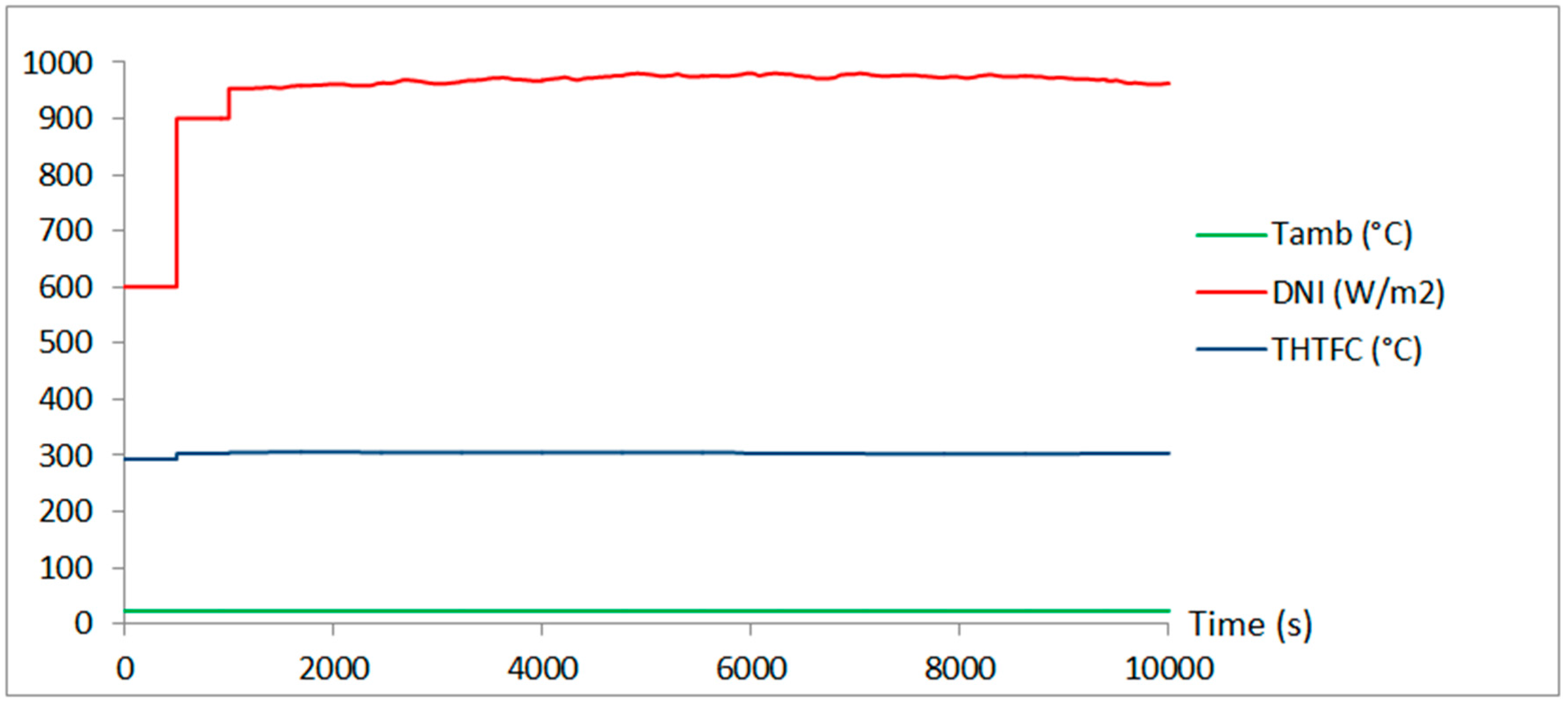
Figure 4.
Evolution of the modeling process.
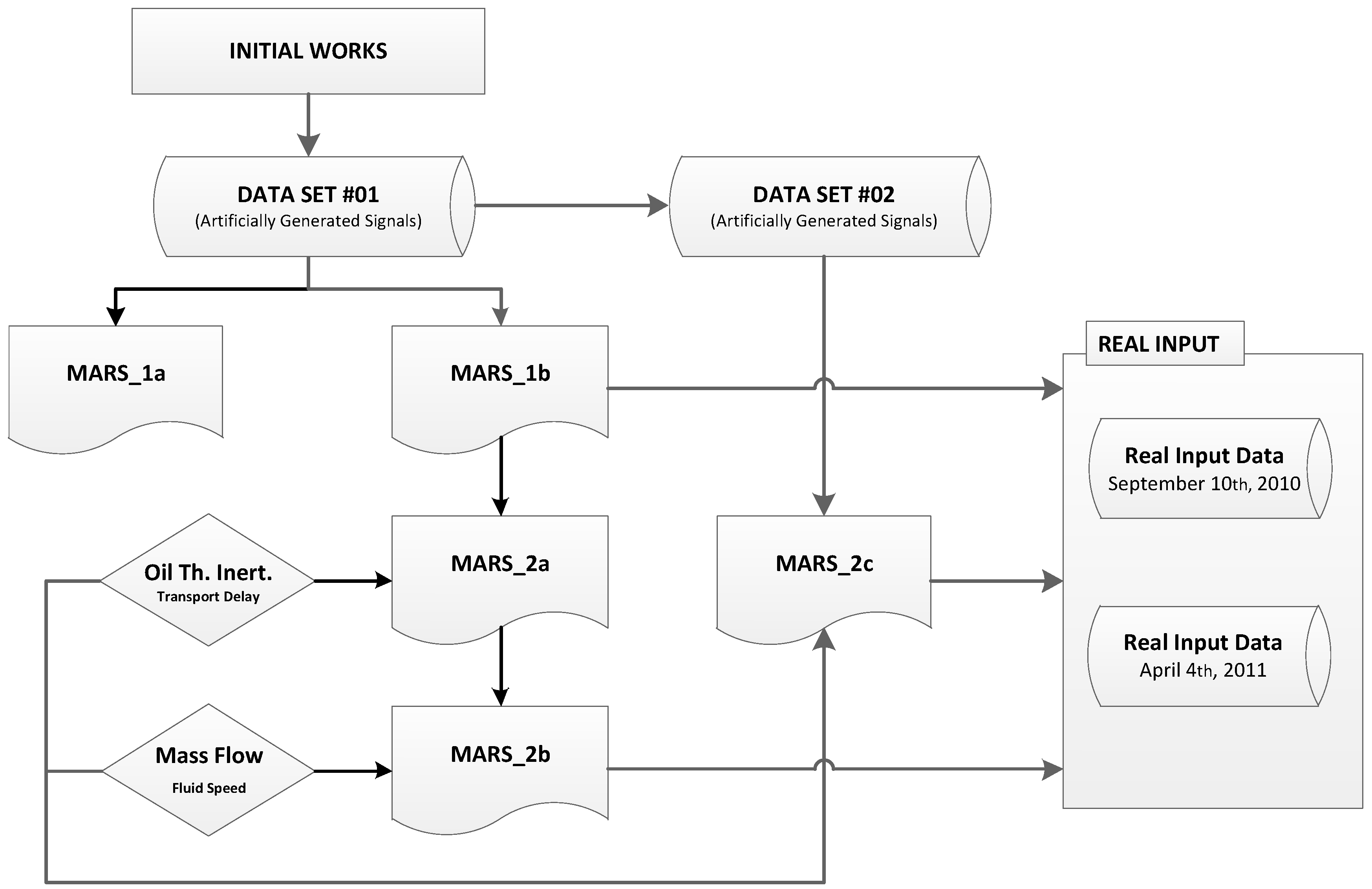
Figure 5.
Graphical representation of the terms that constitute the MARS model: (a) first-order term of the variable mHTF (kg/s); (b) first-order term of the variable THTFC (cold HTF temperature in °C); (c) second-order term of the variables mHTF and ambient temperature; (d) second-order term of the variables mHTF and DNI (W/m2); and (e) second-order term of the variables mHTF and THTFC (cold HTF temperature).

Figure 6.
Comparison between the MARS model and real input data—September 2010.
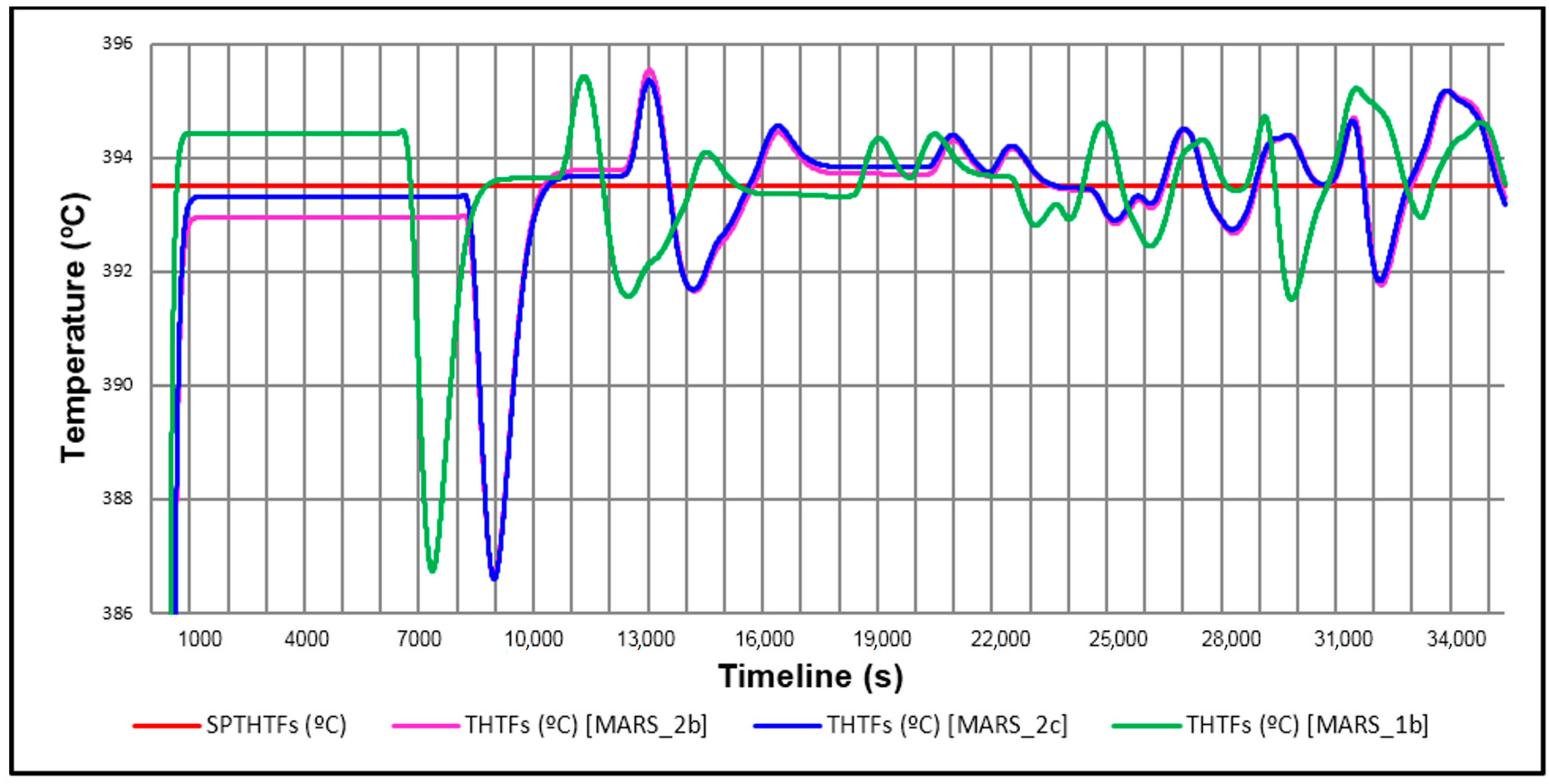
Figure 7.
Comparison between MARS models and real input data—April 2011.

Table 1.
Data organization. HTF: heat transfer fluid.
| Process Inputs | Process Output | Disturbances |
|---|---|---|
| THTFC—Cold HTF Temperature mHTF—HTF Mass Flow | THTFH—Hot HTF Temperature | DNI—Solar Irradiation Tamb—Ambient Temperature Ws—Wind Speed ϕ—Incidence Angle |
Table 2.
Multivariate adaptive regression splines (MARS) models.
| Model | Main Features | Training Data |
|---|---|---|
| MARS_1a | Standard Initial Model (SIM) | Artificial signals (sinusoidal, pulses) |
| MARS_1b | Standard Initial Model (SIM) | Artificial signals (sinusoidal, pulses, sharp step in DNI and knowledge from MARS_1A) |
| MARS_2a | SIM plus thermal inertia effect | Artificial signals (sinusoidal, pulses) and optimized knowledge from MARS_1B |
| MARS_2b | SIM plus mass flow effect | Artificial signals (sinusoidal, pulses, sharp step in DNI and optimized knowledge from MARS_2A) |
| MARS_2c | SIM plus thermal inertia and mass flow effects | Artificial signals (sinusoidal, pulses, sharp step in DNI and optimized knowledge from MARS_2B) |
Table 3.
First MARS models’ responses to a sharp step in DNI. THTF: heat transfer fluid temperature.
Table 3.
First MARS models’ responses to a sharp step in DNI. THTF: heat transfer fluid temperature.
| Response | THTFmin (°C) | THTFmax (°C) | Delay Time (s) 1 | Time to THTFmax 2 | Settling Time (s) 3 |
|---|---|---|---|---|---|
| MARS_1a | 387.50 | 395.20 | 20 | 1500 | 1100 |
| MARS_1b | 366.00 | 392.97 | 17 | 1100 | 1100 |
| MARS_2a | 392.25 | 395.34 | 2 | 1980 | 1980 |
| MARS_2b | 393.09 | 393.71 | 0 | 402 | 2083 |
| MARS_2c | 391.97 | 392.92 | 0 | 566 | 1935 |
1 Average time among the increase until the output starts to react; 2 Average time among the increase until the oil reaches its maximum temperature; 3 Average time among the increase until the output comes to the permanent regime.
Table 4.
Controllers’ response to the sharp step in DNI.
| Model | THTFmax (°C) | THTFmin (°C) | Settling Time (s) | Error (%) |
|---|---|---|---|---|
| PID | 488.00 | 393.01 | 33,000 | 0.0025 |
| PIDFF | 393.70 | 393.01 | 7250 | 0.0025 |
| MARS_2b | 393.71 | 393.33 | 2083 | 0.0840 |
| MARS_2c | 393.07 | 392.97 | 1935 | 0.0178 |
Table 5.
List of the base functions of the MARS model and their coefficients (ci).
| THTFH i | Definition | Ci |
|---|---|---|
| THTFH 1 | 1 | 433.8601 |
| THTFH 2 | h (mHTF-424) | −0.8421 |
| THTFH 3 | h (mHTF-538) | 2.6682 |
| THTFH 4 | h (mHTF-565) | −1.7243 |
| THTFH 5 | h(mHTF-843) | −0.1587 |
| THTFH 6 | h (1190-mHTF) | −0.0615 |
| THTFH 7 | h (mHTF-1190) | 0.0500 |
| THTFH 8 | h (293-THTFe) | 1.0003 |
| THTFH 9 | h (THTFe-293) | −0.0371 |
| THTFH 10 | h (1190-mHTF) × h (Tamb-30) | 0.0082 |
| THTFH 11 | h (1190-mHTF) × h (30-Tamb) | 0.0004 |
| THTFH 12 | h (1190-mHTF) × h (DNI-484) | −0.0002 |
| THTFH 13 | h (1190-mHTF) × h (484-DNI) | 0.0000 |
| THTFH 14 | h (1190-mHTF) × h (DNI-778) | 0.0001 |
| THTFH 15 | h (1190-mHTF) × h (THTFe-283) | 0.0018 |
| THTFH 16 | h (1190-mHTF) × h (283-THTFe) | −0.0009 |
Table 6.
Controllers’ responses to real solar field (SF) data (April 2011). PID: proportional–integral–derivative; PIDFF: PID with feed-forward.
Table 6.
Controllers’ responses to real solar field (SF) data (April 2011). PID: proportional–integral–derivative; PIDFF: PID with feed-forward.
| Model | THTFmax (°C) | THTFmin (°C) | Errormax (%) | Errormin (%) | Total Error (%) |
|---|---|---|---|---|---|
| PID | 401.85 | 367.81 | 2.25 | −6.41 | 8.66 |
| PIDFF | 395.90 | 390.40 | 0.74 | −0.66 | 1.40 |
| MARS_2b | 395.89 | 390.20 | 0.74 | −0.71 | 1.45 |
| MARS_2c | 396.09 | 390.60 | 0.79 | −0.61 | 1.40 |
© 2017 by the authors. Licensee MDPI, Basel, Switzerland. This article is an open access article distributed under the terms and conditions of the Creative Commons Attribution (CC BY) license (http://creativecommons.org/licenses/by/4.0/).
Share and Cite
MDPI and ACS Style
Rogada, J.R.; Barcia, L.A.; Martinez, J.A.; Menendez, M.; De Cos Juez, F.J. Comparative Modeling of a Parabolic Trough Collectors Solar Power Plant with MARS Models. Energies 2018, 11, 37. https://doi.org/10.3390/en11010037
AMA Style
Rogada JR, Barcia LA, Martinez JA, Menendez M, De Cos Juez FJ. Comparative Modeling of a Parabolic Trough Collectors Solar Power Plant with MARS Models. Energies. 2018; 11(1):37. https://doi.org/10.3390/en11010037
Chicago/Turabian StyleRogada, Jose Ramón, Lourdes A. Barcia, Juan Angel Martinez, Mario Menendez, and Francisco Javier De Cos Juez. 2018. "Comparative Modeling of a Parabolic Trough Collectors Solar Power Plant with MARS Models" Energies 11, no. 1: 37. https://doi.org/10.3390/en11010037
Note that from the first issue of 2016, this journal uses article numbers instead of page numbers. See further details here.