Rate Decline Analysis for Modeling Volume Fractured Well Production in Naturally Fractured Reservoirs


Research Institute of Petroleum Exploration and Development, PetroChina, Beijing 100083, China
*
Author to whom correspondence should be addressed.
Energies 2018, 11(1), 43; https://doi.org/10.3390/en11010043
Submission received: 20 October 2017
/
Revised: 27 November 2017
/
Accepted: 21 December 2017
/
Published: 1 January 2018
(This article belongs to the Special Issue Mathematical and Computational Modeling in Geothermal Engineering)
Abstract
:Based on the property discontinuity in the radial direction, this paper develops a new composite model to simulate the productivity of volume fractured wells in naturally fractured reservoirs. The analytical solution of this model is derived in detail and its accuracy is verified by the same model’s numerical solution. Detailed analyses of the traditional transient and cumulative rate are provided for the composite model. Results show that volume fracturing mainly contributes to the early-flow period’s production rate. As interregional diffusivity ratio increases or interregional conductivity ratio decreases, the transient rate at the same wellbore pressure increases. Three characteristic decline stages may be observed on transient rate curves and the shape of traditional rate curves in the middle- and late-flow periods depends on naturally fractured medium and boundary condition. By introducing a new pseudo-steady constant, new Blasingame type curves are also established and their features are more salient than those of traditional rate curves. Five typical flow regimes can be observed on these new type curves. Sensitivity analysis indicates that new Blasingame type curves for varied interregional diffusivity ratio, interregional conductivity ratio, interporosity coefficient and dimensionless reservoir radius, except storativity ratio, will normalize in the late-flow period.
1. Introduction
Volume fracturing has been an effective technique to enhance the productivity of the wells with damaged zones or in low-permeability formations. Production wells in naturally fractured reservoirs are a potential target for being stimulated by such technique. After volume fracturing treatment, a certain stimulated region composed of hydraulic fractures, natural fractures and shear cracks is created near the wellbore. This reduces the flow resistance and thus improves the wells’ production [1,2]. However, it is difficult to test and evaluate the productivity under such complex fracture network conditions caused by volume fracturing.
As an important method, rate decline analysis is widely used to predict well performance and estimate reservoir properties. In terms of productivity analysis and prediction, Arps [3] generalized the production decline law into three types: exponential decline, harmonic decline, and hyperbolic decline. Fetkovich [4] proved Arps’ rate decline law theoretically and combined theoretical decline curves with Arps decline equations to further analyze rate decline. However, Fetkovich type curves could not solve the problem of both variable production rate and variable wellbore pressure. Blasingame et al. [5,6] solved this problem skillfully by introducing the concepts of material balance time and rate integral average. Later, Fetkovich and Blasingame type curves were extended into other well types, such as fractured wells and horizontal wells [7,8,9,10,11,12].
Based on the assumption that the well is intersected by a single fracture, Gringarten et al. [13] developed three important solutions for fractured wells: infinite-conductivity fracture solution, uniform-flux fracture solution for the well with a vertical fracture, and uniform-flux fracture solution for the well with a horizontal fracture. Later, Cinco-Ley et al. [14] provided a semi-analytical solution for the well with a finite-conductivity vertical fracture. These four solutions have a significant effect on the study of fractured wells, but all the solutions are limited to the transient-pressure analysis. Based on their solutions, a few scholars began to conduct the rate decline analysis of fractured wells by using the approaches originally proposed by Fetkovich and Blasingame [4,5,6]. Wang et al. [15] established Blasingame type curves for the well with a finite-conductivity vertical fracture in tight oil reservoirs and investigated its productivity. Further, Wang et al. [16] considered the fracture face damage existed in a finite-conductivity vertical fracture and also developed rate decline curves like Blasingame to discuss the effect of fracture face damage. It has been shown that the increase in the productivity of a fractured well depends on fracture characteristics, such as fracture conductivity, length, and penetration [17,18].
The previous studies assume that only a single fracture intercepts the wellbore. However, in practice, a few observations from the field and laboratory have shown very complex fracture paths and the presence of multiple fractures, multi-segmented fractures and branchings [19,20,21,22,23,24]. Multiple fractures can occur near the wellbore and they grow out of each other’s influence zone [20,25,26]. Therefore, the previous assumption about hydraulic fracture near the wellbore is not valid in the case of volume fractured wells in naturally fractured reservoirs. When a reservoir has a discontinuity of material properties in the radial direction, it can be considered a composite reservoir [27]. Volume fracturing treatment creates a high-permeability region near the wellbore, for this reason, the case of a well with multiple complex fractures near the wellbore in naturally fractured reservoirs can be closely represented by a composite reservoir model. Restrepo [28] also developed an analytical model for multiple fractures with complex geometry to investigate the transient pressure by using superposition principle, which puts forward a new way to deal with the complex fracture network. Unfortunately, he does not include the well productivity in his work.
Due to the good stimulation of volume fracturing, rate decline analysis in volume fractured well production has attracted a continuous increasing attention. Al-Salem et al. [29] established a numerical model by using a vertical and horizontal orthogonal fracture network to approximately substitute the volume reconstruction. Combining with the micro seismic exploration results, Arvind et al. [30] approximately simulated the reconstruction region around the wells. Using the fractal theory, Liu et al. [31,32] and Xiao and Zhao [33] described the fracture distribution in the stimulated region and presented an analytical model to simulate the productivity of cold and heavy oil. However, to be my best known, there is still no overall well test interpretation model and rate decline type curves for vertical wells with volume fracturing in naturally fractured reservoirs.
The purpose of this work is to simulate the productivity of volume fractured wells in naturally fractured reservoirs by establishing rate decline type curves. Firstly, based on the concept of composite reservoir, this paper develops a new mathematical model for volume fractured well production in such reservoirs. Secondly, we acquire the analytical solution of this composite model in Laplace space and verify its accuracy through comparing it with the same model’s numerical solution. Thirdly, we compare the differences of productivity between the models with and without volume fracturing and also investigate the parameter influence on the traditional transient and cumulative rate curves thoroughly. Finally, we establish new Blasingame type curves by using a new pseudo-steady constant, and identify main flow regimes on the new Blasingame type curves and further emphatically discuss parameter sensitivity of these type curves, including interregional diffusivity ratio, interregional conductivity ratio, storativity ratio, interporosity coefficient and dimensionless reservoir radius.
2. Analytical Solution to Mathematical Model
Figure 1 shows a sketch of the flow of a volume fractured well in a naturally fractured reservoir. A stimulated region with joint network is formed in the near-wellbore area after volume fracturing treatments (Figure 1a). Using the concept of composite reservoir, the proposed model can be normally subdivided into two concentric regions: the inner region with multiple fractures (Region I) and the outer region with naturally fractured formation (Region II), respectively (Figure 1b). In the inner region, multiple hydraulic fractures caused by volume fracturing greatly improve the connectivity and conductivity near the wellbore, thus we can assume that these fractures have infinite conductivity, and fluid seepage in them follows Darcy linear flow. We use the classical Warren-Root model [34] to describe the fluid flow in the outer region. In order to establish a mathematical model, certain simplifications and assumptions in the composite model are made (Figure 1c):
- (1)
- All the hydraulic fractures, with the same properties, fully penetrate the formation, and the reservoir is closed at the external boundary of side and bounded by upper and lower impermeable formation.
- (2)
- Flow in the reservoir is considered to be a single-phase flow with slightly compressible fluid of constant viscosity and volume factor.
- (3)
- The joint fracture network constituted the main flow channel in the composite system, and fluid flow in the reservoir is laminar and isothermal. In the inner region, fluid flows into the wellbore only through hydraulic fractures and the matrices of this region have no contribution to the flow; in the outer region, fluid first flows from the matrices to the natural fractures and then directly flows into the hydraulic fractures of the inner region.
- (4)
- A vertical well intercepted by a finite number of hydraulic fractures is located at the center of the composite reservoir. No wellbore storage effect and skin effect is considered.
Based on the composite model above, we can establish a mathematical model for volume fractured wells in naturally fractured reservoirs (seen in Appendix A). Flow patterns in the inner and outer regions are defined first. Considering the continuity of pressure and flux at the interface, two interface conditions are then incorporated into the model. To simplify the problem, we do the nondimensionalization and Laplace transform for the mathematical model successively.
Note that the governing equations, Equations (A7) and (A18), are the typical Bessel equations. Their general solutions in Laplace space can be given by:
respectively.
Combining the boundary conditions (Equations (A8) and (A19)) and interface conditions (Equations (A24) and (A25)) with the general solutions, we can obtain the following mathematical Equations:
By solving the equations, we can acquire the wellbore pressure in Laplace space:
where: , .
According to Duhamel principle [35], the pressure solution under constant rate and the rate solution under constant wellbore pressure have the following correlation in Laplace space:
Furthermore, using the relationship between the transient and cumulative rates, we can obtain the cumulative rate under constant wellbore pressure in Laplace space:
Then, combining Equations (4)–(6), , and for any given in real space can be figured out by the Stehfest numerical inverse method [36].
3. Verification of the Analytical Solution
As far as we know, in the literature there is no other analytical model dealing with volume fractured wells in naturally fractured reservoirs. Generally, a model’s numerical solution is an effective way to verify its analytical solution’s accuracy. Numerical solution of this composite model can be obtained by solving a tri-diagonal matrix, which can be constructed by treating the dimensionless mathematical model (seen in Appendix A) with a finite difference method and simultaneously introducing a mirror image method to deal with the dimensionless boundary and interface conditions [37]. Therefore, we can verify the accuracy of the analytical solution through comparing it with the numerical solution. Figure 2 shows the comparison results of two solutions under different interregional diffusivity ratio, interregional conductivity ratio, fracture-matrix storativity ratio, and fracture-matrix interporosity coefficient, respectively. The excellent agreement within the most production life between our analytical and numerical solution results can be seen in this figure. These comparisons indicate that the analytical solution in this paper is reliable, thus we can proceed with the development of rate decline curves using the analytical solution. It is noteworthy that these two kinds of solutions have their own advantages. The computational speed of the numerical solution is faster than that of the analytical solution, but the analytical solution is easier to take the wellbore storage and skin effects into consideration and also more convenient to conduct the rate decline analysis by using Duhamel principle.
4. Results and Discussion
In this section, we conduct a detailed productivity analysis for a volume fractured well in the naturally fractured reservoir, including differences of well productivity between the reservoir models with and without volume fracturing, parameter influence on traditional transient and cumulative rate curves, flow regime recognition on new Blasingame type curves and sensitivity analysis of new Blasingame type curves.
4.1. Comparison with a Model not Having Volume Fracturing
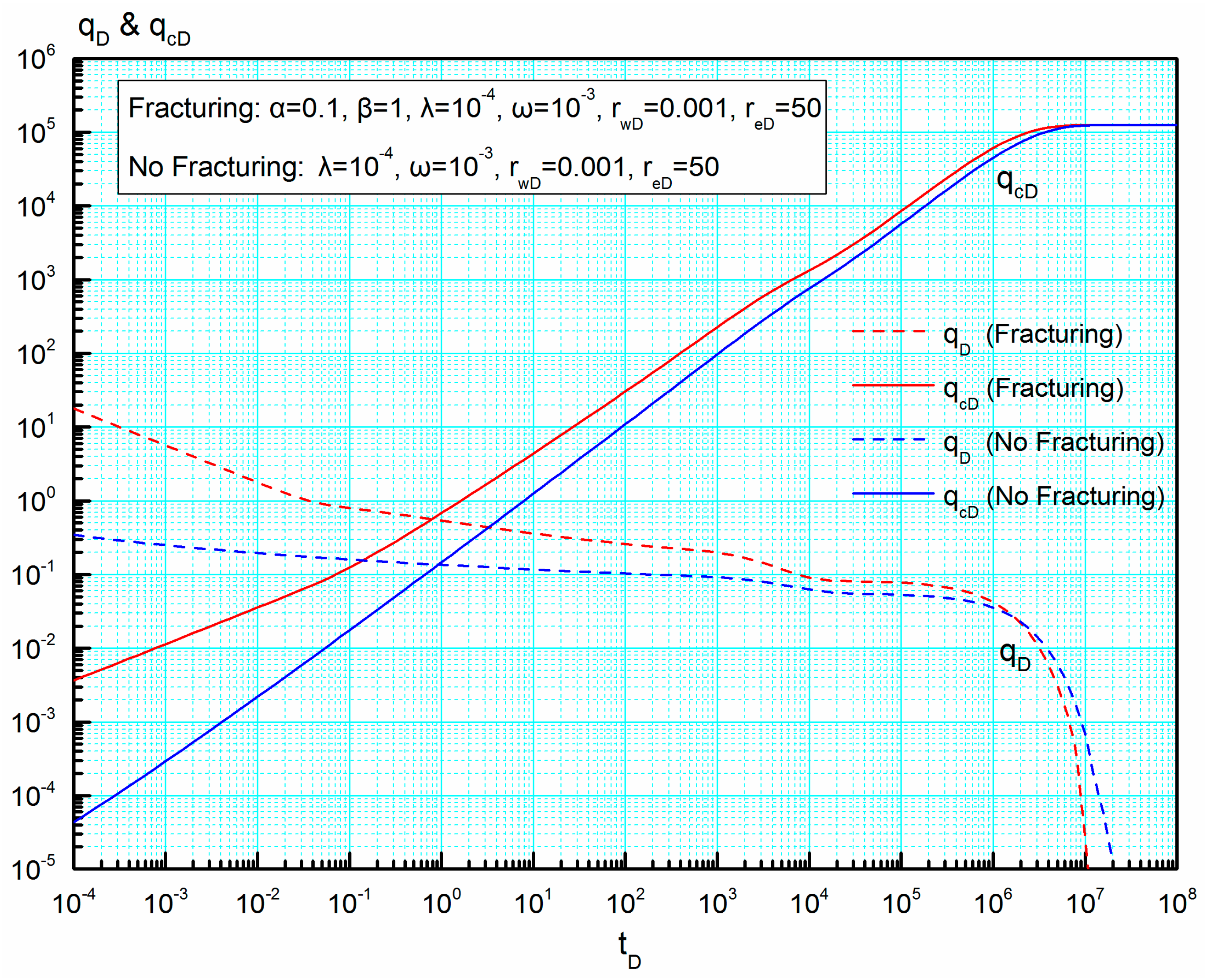
Since we have established an analytical model for a volume fractured well in the naturally fractured reservoir, it is necessary to make a comparison of this model with the same reservoir model not having volume fracturing to know their differences. Figure 3 presents the differences of the transient and cumulative rate curves between these two models. It can be seen that the same parameters for two models are ω, λ, rwD and reD, but the parameters α and β, only belong to the model with volume fracturing.
As shown in Figure 3, in the early and middle time both the transient and cumulative rates of the volume fractured well are higher than those of the well without the stimulation at the same group of production parameters, due to a larger drainage area caused by volume fracturing. However, in the late time, the transient rate of the volume fractured well is slightly lower than that of the well without the stimulation, but this difference can be ignored because the transient rate is very low in the later time. It also can be seen that the rate decline of the volume fractured well is much faster than that of the well without the stimulation and the cumulative rates of these two models reach the same in the late time, which implies that volume fracturing treatment mainly contributes to the early-flow production but has little influence on the final cumulative rate.
4.2. Parameter Influence on Transient and Cumulative Rate Curves
There is a possibility of multiple solutions for well test analysis and the shape of type curves may be affected by different parameter values. Figure 4, Figure 5, Figure 6, Figure 7 and Figure 8 show how the shape of the transient and cumulative rate curves for a volume fractured well in the naturally fractured reservoir is affected by changing the parameters.
4.2.1. Interregional Diffusivity Ratio α and Interregional Conductivity Ratio β
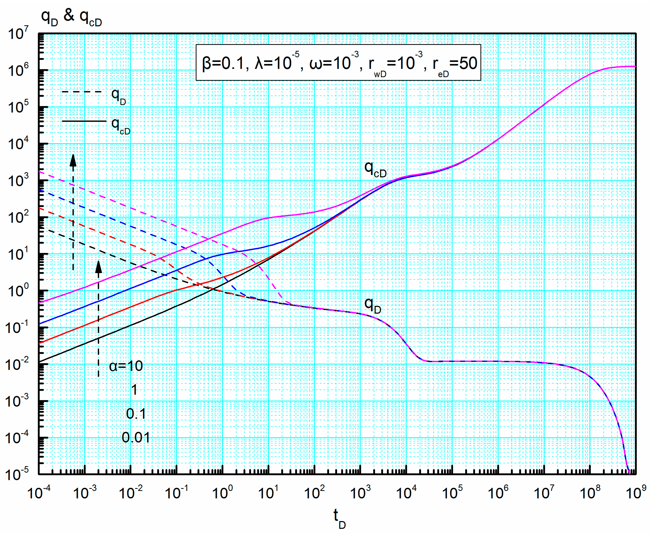
Physically interregional diffusivity ratio α and interregional conductivity ratio β represent two fracture systems’ diffusivity ratio and conductivity ratio, respectively. These two parameters depend on the permeability, the number of hydraulic fractures and the storativity of two fractured regions. Figure 4 and Figure 5 show the effect of these two parameters on the transient and cumulative rates, respectively. There are three characteristic decline stages within the whole production life on the transient rate curves: initially transient rate decreases linearly, then the second decline stage comes after a stable production period, and when the pressure wave spreads to the outer boundary, the third decline stage occurs and the production rate approaches to zero.
From Figure 4, we can find that interregional diffusivity ratio mainly affects the early-flow period and during this period a larger leads to a higher production rate at the same wellbore pressure. In the later-flow period, the diffusion capacity of the inner region well satisfies the demand of fluid flow feeding the wellbore and flow in the composite model reaches a dynamic balance. Therefore, changing interregional diffusivity ratio does not affect the transient rates and the cumulative rates reach the same in the later-flow period.
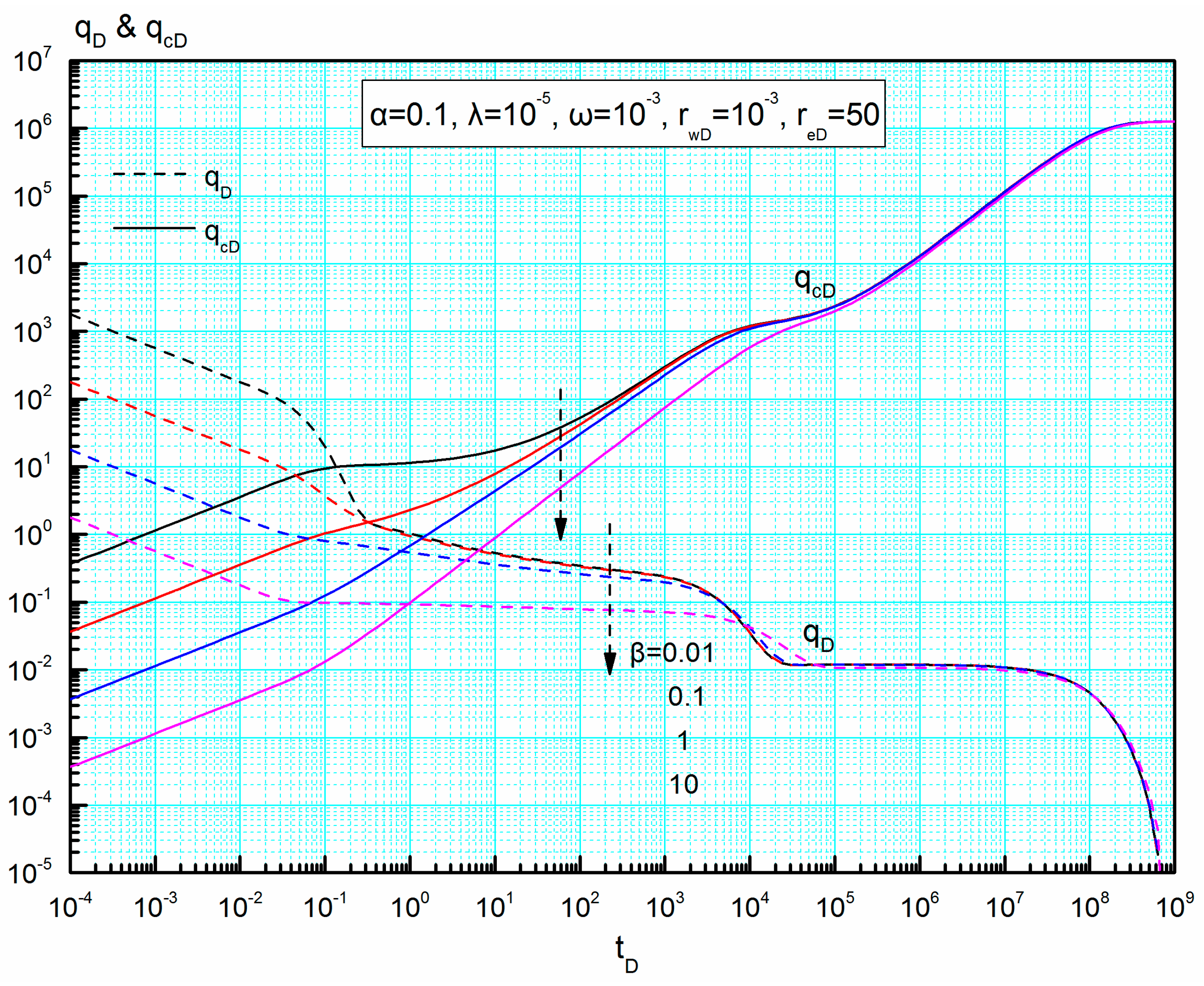
Figure 5 demonstrates that interregional conductivity ratio mainly affects the early- and middle-flow periods and during these periods a larger interregional conductivity ratio corresponds to a lower production rate at the same production. As we know, a larger interregional conductivity ratio means a weaker conductivity of the inner region. Therefore, a larger interregional conductivity ratio increases the flow resistance, which can explain the previous result.
As shown in Figure 4 and Figure 5, in the late-flow period, the transient rate curves normalize for varied interregional diffusivity ratio and interregional conductivity ratio, respectively, and so do the cumulative rate curves for these two parameters. Considering that the parameters α and β only depend on volume fracturing treatment, these normalizations demonstrate that this stimulation technique has no influence on the total productivity but significantly improves the production rate in the early-flow period.
4.2.2. Storativity Ratio ω and Interporosity Coefficient λ
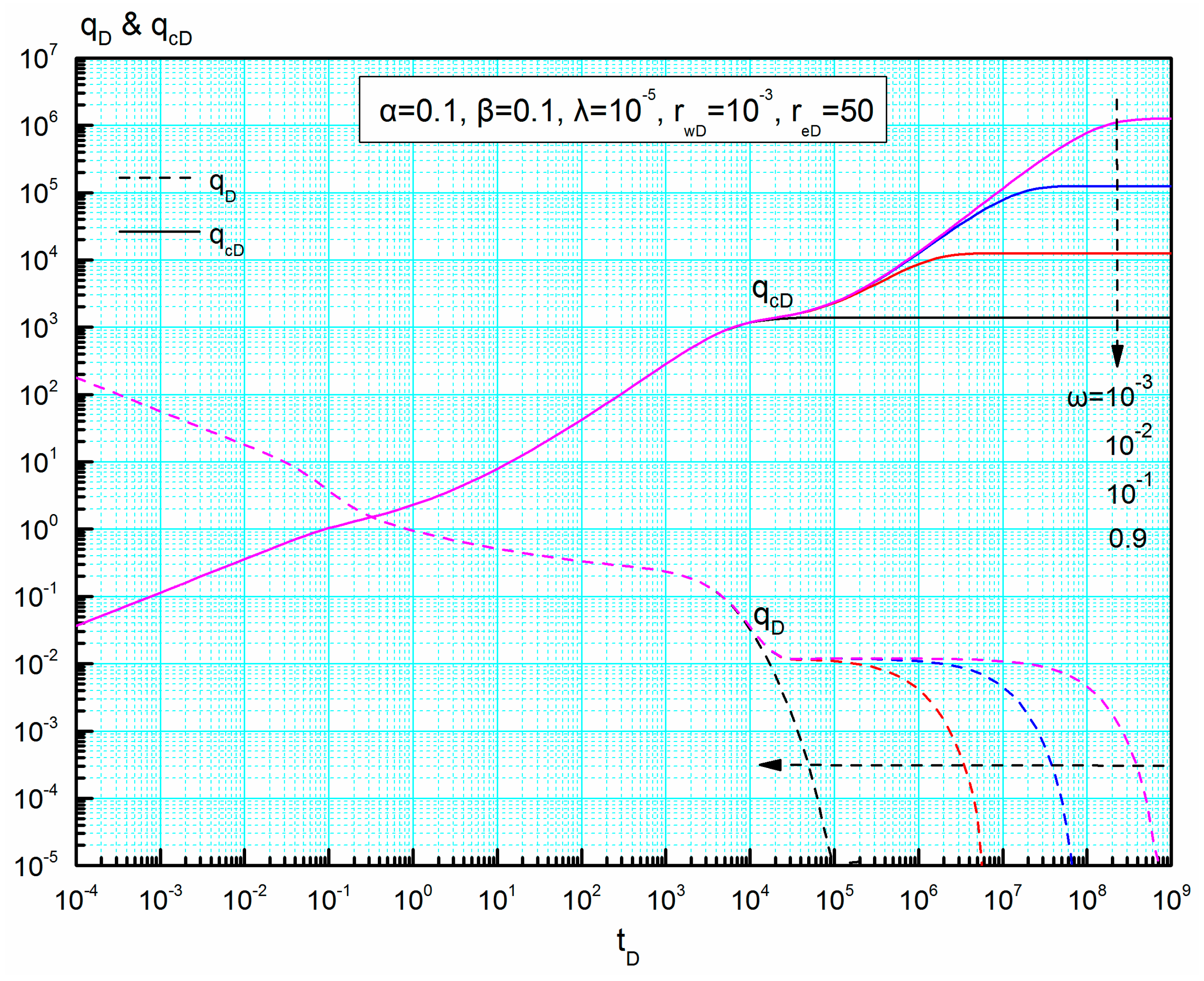
The influence of fracture-matrix storativity ratio (ω = 10−3, 10−2, 10−1 and 0.9) and fracture-matrix interporosity coefficient (λ = 10−6, 10−5, 10−4 and 10−3) on the transient and cumulative rate curves are given in Figure 6 and Figure 7, respectively. It can be seen from these two figures that the storativity ratio and interporosity coefficient only affect the late-flow period, similar to the common dual media. There are also three decline stages on their transient rate curves.
From Figure 6, as storativity ratio increases from 0.001 to 0.9, the third decline stage occurs earlier and the duration of the last stable production stage becomes shorter. This is because when ω goes to 1, reserves in the matrix system approach to zero and inter-porosity flow in the outer region is very weak, which accelerate the rate decline. Note that the final cumulative rate curves are a set of parallel horizontal lines and a higher storativity ratio corresponds to a lower cumulative rate in the late-flow period. As shown in Figure 7, with the increase of interporosity coefficient, the second decline stage lasts short and even disappears from the transient rate curves, but the appearance of the third decline stage gets early and also the transient rate corresponding to this stage decreases. It can be interpreted by that the ability of matrix system supplying fluid for natural fracture system becomes stronger as interporosity coefficient increases. Different from the influence of storativity ratio, this group of cumulative rate curves will normalize in the late-flow period, which suggests that interporosity coefficient has no influence on the final cumulative rate
4.2.3. Dimensionless Reservoir Radius reD
In this paper, we focus on the case of closed boundary. Figure 8 presents the influence of dimensionless reservoir radius on the transient and cumulative rate curves (reD = 50, 100, 200 and 400). There is no difference in the shape of type curves in the early- and middle-flow periods under varied dimensionless reservoir radius. However, in the late-flow period, as the parameter reD decreases, both the transient and cumulative rates decrease rapidly, which meets the characteristic of closed reservoir.
4.3. Flow Regime Recognition on Blasingame Type Curves
For closed external boundary, the late-time behavior of well production corresponds to a pseudo-steady flow. Specially, we further study the pseudo-steady analytical solution by means of the asymptotic analysis method.
As (), considering these approximate relations in Equation (4) and then conducting the Laplace inverse, a new pseudo-steady analytical formula in real space can be obtained:
Recalling the general identity for pseudo-steady flow under the dimensionless condition [4,10], we can define bDpss as a new dimensionless pseudo-steady constant for our composite model, which is given by:
where the parameter bDpss is independent of time, but is a function of reD. In fact, bDpss is close to a constant when reD is large enough. The work to derive the variable bDpss is essential for the development of new rate decline curves. The bDpss parameter always acts as a correlating variable when we define some new rate functions [4].
In order to eliminate the possibility of multiple solutions and reduces the errors in well test analysis, Blasingame et al. [6] created the integral average method of rate and defined the following two variables, which are widely used in the rate decline analysis:
- (1)
- Dimensionless rate integral function: qDdi
- (2)
- Dimensionless rate integral derivative function: qDdid
Now incorporating Equations (13)–(16) with our composite model, we can consequently establish new Blasingame type curves for volume fractured well production in the naturally fractured reservoir. New Blasingame type curves are normally composed of log-log plots of rate integral function qDdi and rate integral derivative function qDdid with “decline time” tDd. Due to the addition of rate integral derivative function, it can amplify the small variations in the flow process on type curves and greatly help us to identify its flow behavior, which is a huge advantage of Blasingame type curves over the traditional rate decline type curves.
Figure 9 clearly shows an entire transient flow process for a volume fractured well in the naturally fractured reservoir with closed boundary and five typical flow regimes can be observed on the new Blasingame type curves:
Regime I: linear flow regime. The curves of qDdi and qDdid are a pair of parallel downward straight lines with the slope of negative one half, which is the typical characteristic of linear flow.
Regime II: transition flow regime. This regime occurs when the interface of two regions is felt. The curves of qDdi and qDdid are not parallel.
Regime III: radial flow regime. Production continues to decline while the curves of qDdi and qDdid become a pair of parallel downward sloping lines again. In this regime, fluid flow in the natural fracture and hydraulic fracture systems reaches a dynamic balance.
Regime IV: inter-porosity flow regime. The curve of qDdid is first convex and then concave, which is a reflection of fracture-matrix inter-porosity flow.
Regime V: pseudo-steady flow regime. For a closed boundary, when the pressure wave spreads to the outer boundary, pseudo-steady flow begins to appear in the composite system and the curves of qDdi and qDdid converge to a straight line with negative unit slope.
Type curves’ shape in regime I and II is typical of fluid flow for volume fractured wells. The shape and position of type curves in the early time are dominated by interregional diffusivity ratio α and interregional diffusivity ratio β. Type curves’ shape in regimes IV and V is typical of fluid flow in the naturally fractured reservoir. The shape and location of type curves in the late time are dominated by storativity ratio ω, interporosity coefficient λ and dimensionless reservoir radius reD.
4.4. Sensitivity Analysis of New Blasingame Type Curves
Compared with the traditional rate decline curves, Blasingame type curves could deal with the issue of both variable rate and variable wellbore pressure. It is useful and necessary to establish a set of Blasingame type curves for volume fractured well production in the naturally fractured reservoirs. Figure 10, Figure 11, Figure 12, Figure 13 and Figure 14 contain these new type curves for different parameter conditions. Later we will show the results of sensitivity analysis of new Blasingame type curves.
4.4.1. Interregional Diffusivity Ratio
Figure 10 presents the effect of interregional diffusivity ratio on dimensionless rate integral qDdi and dimensionless rate integral derivative qDdid. The curves of qDdi and qDdid have the same decline trend, but the features of the qDdid curves are more salient than those of the qDdi curves. As shown in Figure 10, the values of qDdi and qDdid before inter-porosity flow regime decrease as interregional conductivity ratio decreases. We can find that this parameter mainly affects the early-flow period and radial flow regime may be absent at a large interregional diffusivity ratio. Meanwhile, as the value of α decreases, the duration of linear flow regime is shortened while that of transition flow regime is prolonged. When interregional diffusivity ratio is larger than 1, fluid velocity in the inner region is slower than that in the outer region. Additionally, all the new type curves for different interregional diffusivity ratio will normalize at the start of inter-porosity flow regime.
4.4.2. Interregional Conductivity Ratio β
Blasingame type curves for different interregional conductivity ratio are shown in Figure 11. Before inter-porosity flow regime, a larger the interregional conductivity ratio corresponds to smaller values of qDdi and qDdid.
It can be concluded that the effect of interregional conductivity ratio is predominantly on linear-, transition- and radial-flow regimes. When the value of β is low enough, radial flow may be absent and replaced by transition flow. With the increase of interregional conductivity ratio, the duration of linear flow is shortened while that of radial flow is prolonged. Interestingly, all the curves of qDdi and qDdid for varied interregional conductivity ratio will normalize in the pseudo-steady flow regime
4.4.3. Storativity Ratio ω
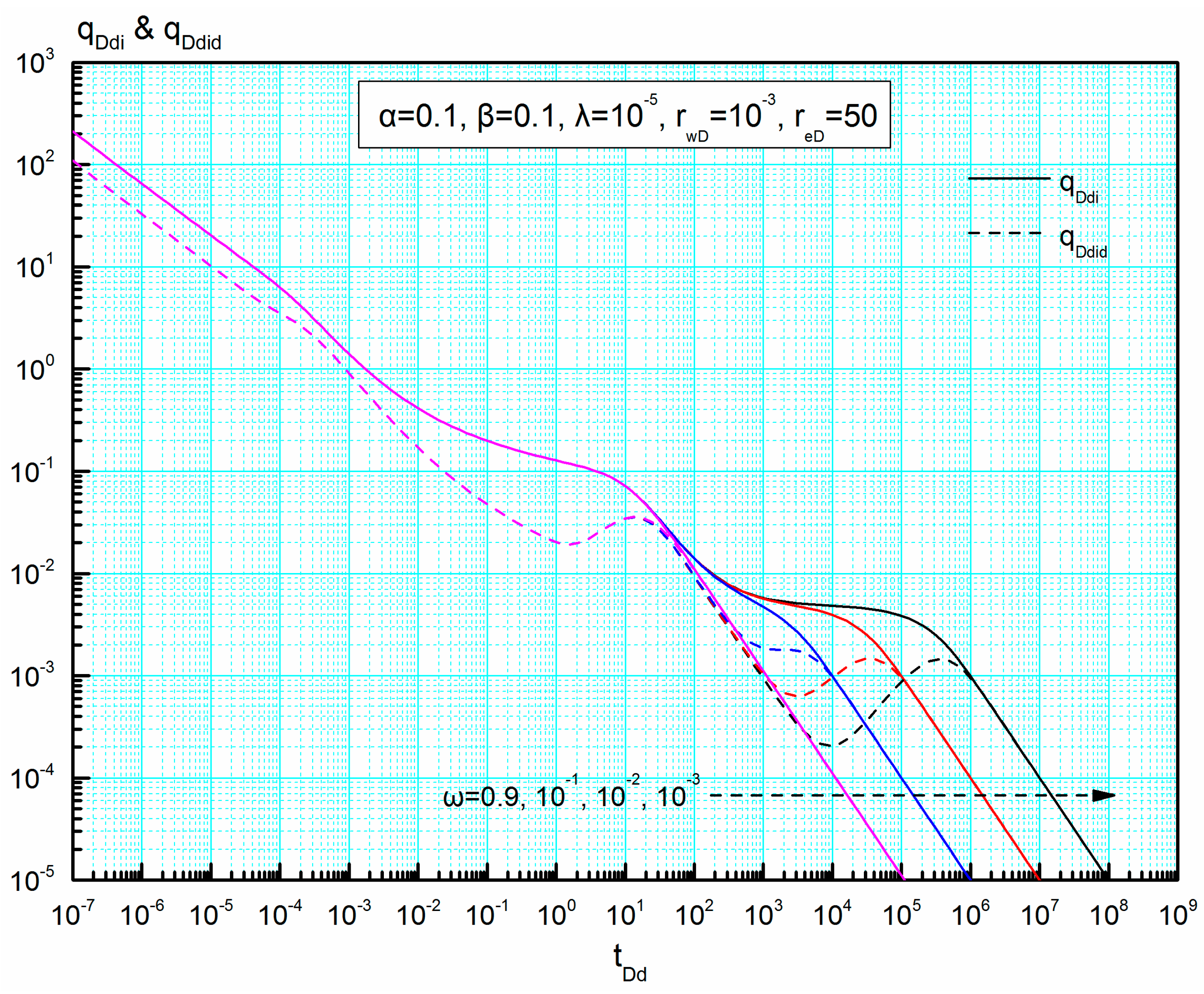
Figure 12 shows the effect of storativity ratio on the curves of qDdi and qDdid. Similar to the common naturally fractured media, it can be observed that storativity ratio has a strong influence on the inter-porosity flow regime and the curves of qDdid are concave in this regime. With the decrease of storativity ratio, the inter-porosity flow becomes more obvious, the duration of this regime becomes longer, and also the values of both qDdi and qDdid becomes lower. It is worth noting that a larger storativity ratio corresponds to a smaller valley value of qDdid in the inter-porosity flow regime. In the late-flow period, the curves of qDdi and qDdid corresponding to each storativity ratio will normalize, respectively, which is different from the influence of the other four parameters on the Blasingame type curves.
4.4.4. Interporosity Coefficient λ
From Figure 13, we can see that interporosity coefficient λ also mainly affects the duration and degree of inter-porosity flow, like the common dual media. The lower the interporosity coefficient is, the longer the inter-porosity flow regime lasts. Meanwhile, the values of both qDdi and qDdid in the inter-porosity flow regime decrease with the decrease of interporosity coefficient. Similarly, the curves of both qDdi and qDdid normalize in the pseudo-steady flow regime.
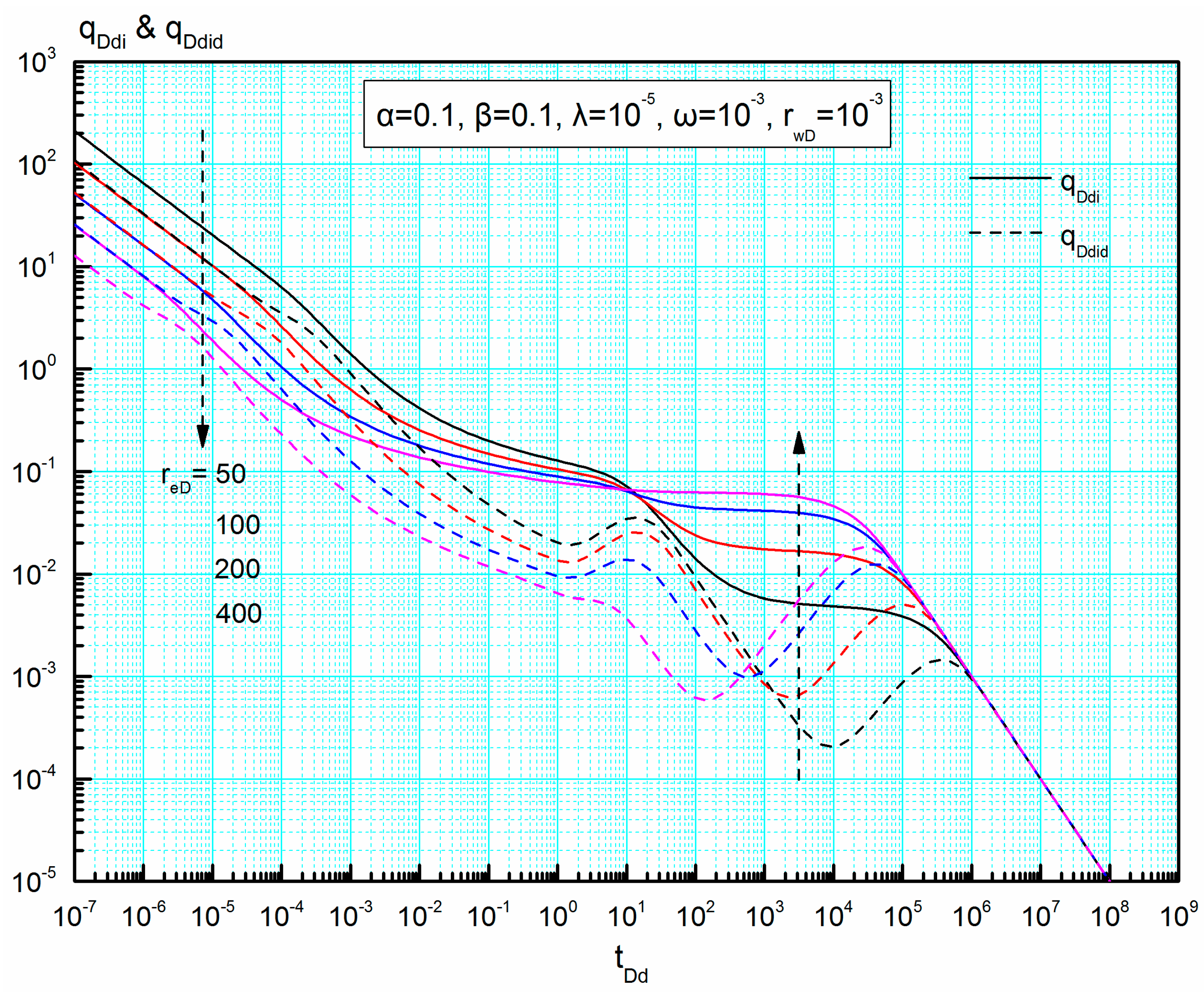
4.4.5. Dimensionless Reservoir Radius reD
Blasingame type curves for different dimensionless reservoir radius are given in Figure 14. The difference in the shape of new Blasingame type curves for varied reD appears in the early-flow period and the curves of both qDdi and qDdid normalize in the pseudo-steady flow regime, which is contrary to the traditional rate decline curves (Figure 8).
For different reD, the features of new Blasingame type curves are more salient than those of traditional rate decline curves. Therefore, these new type curves are convenient for us to quickly detect the radius of closed reservoir by using field data. Before the inter-porosity flow regime, both the dimensionless rate integral and dimensionless rate integral derivative decrease as the parameter reD increases.
5. Conclusions
This paper presents a new composite model for rate decline analysis of volume fractured wells in naturally fractured reservoirs. Based on this work, several important conclusions are obtained:
- Compared with the model not having volume fracturing, this stimulation technique mainly contributes to the early-flow period’s production.
- Three characteristic decline stages and two stable production periods may be observed on the transient rate curves. In the early-flow period, the transient rate at the same wellbore pressure increases as interregional diffusivity ratio increases or interregional conductivity ratio decreases. In the middle- and late-flow periods, the shape of the traditional rate curves depends on naturally fractured medium and boundary condition.
- New Blasingame type curves for volume fractured wells in naturally fractured reservoirs are established and can be used to deal with the problem of both variable rate and variable wellbore pressure. Five flow regimes may be observed on the new Blasingame type curves: linear flow regime, transition flow regime, radial flow regime, inter-porosity flow regime, and pseudo-steady flow regime. The shape and position of type curves in linear- and transition-flow regimes are predominantly determined by interregional diffusivity ratio and interregional conductivity ratio.
- New Blasingame type curves have more salient features and better normalizations than the traditional rate curves and are convenient for us to conduct well testing analysis. Sensitivity analysis indicates that these new type curves for varied interregional diffusivity ratio, interregional conductivity ratio, interporosity coefficient and dimensionless reservoir radius, except storativity ratio, will normalize in the late-flow period.
Acknowledgments
The authors thank the National Science and Technology Major Project of China (No. 2017ZX05030-002) for financial support.
Author Contributions
All authors have contributed to this work. Mingxian Wang and Guoqiang Xing proposed the original idea for this paper. Mingxian Wang, Guoqiang Xing, Wenqi Zhao and Penghui Su contributed to the modeling, programming, and results analysis and discussion. This paper was written by Mingxian Wang and modified by Guoqiang Xing, Heng Song and Penghui Su. Zifei Fan provided technical guidance for the whole research work.
Conflicts of Interest
The authors declare no conflict of interest.
Nomenclature
Field Variables
| k | permeability, m2 |
| h | formation thickness, m |
| μ | fluid viscosity, Pa·s |
| p | pressure, Pa |
| r | radial distance, m |
| rf | half length of artificial fracture, m |
| b | aperture of artificial fracture, m |
| t | time variable, s |
| porosity, fraction | |
| ct | compressibility factor, Pa−1 |
| q | total rate at the wellbore, m3/s |
| B | volume factor, m3/m3 |
| γ | shape factor, dimensionless |
| η | fluid transmissivity factor, Pa·m2/(Pa·s) |
| n | number of artificial fractures, dimensionless |
| π | 3.1415926…… |
Dimensionless Variables: Real Domain
| rD | dimensionless radius |
| reD | dimensionless drainage radius |
| rwD | dimensionless wellbore radius |
| tD | dimensionless time |
| tDd | dimensionless decline time |
| bDpss | dimensionless pseudo-steady constant |
| p1D | dimensionless pressure in the inner region |
| pwD | dimensionless wellbore pressure |
| p2fD | dimensionless pressure of natural fracture system |
| p2mD | dimensionless pressure of matrix system |
| pwD,pss | dimensionless wellbore pressure in pseudo-steady flow regime |
| qwD | dimensionless transient rate |
| qcD | dimensionless cumulative rate |
| qDd | dimensionless decline rate |
| qDdi | dimensionless rate integral |
| qDdid | dimensionless rate integral derivative |
Dimensionless Variables: Laplace Domain
| s | time variable in Laplace domain |
| x1 | corresponding coefficient in Laplace domain |
| x2 | corresponding coefficient in Laplace domain |
| dimensionless pressure p1D in Laplace domain | |
| dimensionless wellbore pressure pwD in Laplace domain | |
| dimensionless pressure p2fD in Laplace domain | |
| dimensionless transient rate qwD in Laplace domain | |
| dimensionless cumulative rate qcD in Laplace domain |
Greek Variables
| α | interregional diffusivity ratio |
| β | interregional conductivity ratio |
| ω | fracture-matrix storativity ratio |
| λ | fracture-matrix interporosity coefficient |
Special Functions
| I0(x) | modified Bessel function (1st kind, zero order) |
| I1(x) | modified Bessel function (1st kind, first order) |
| K0(x) | modified Bessel function (2nd kind, zero order) |
| K1(x) | modified Bessel function (2nd kind, first order) |
Special Subscripts
| D | dimensionless |
| w | wellbore |
| e | reservoir external boundary |
| 1 | inner region |
| 2f | natural fracture in the outer region |
| 2m | matrix in the outer region |
| i | initial or ordinal |
Appendix A. Establishment of Mathematical Model
Appendix A.1. Flow in the Inner Region
A finite number, n, of hydraulic fractures constitute the main flow channel in the inner region and flow in each fracture has been assumed to be linear, thus the flow equation for the inner region can be written as:
Initial condition:
Well production condition at constant rate production:
Introducing the dimensionless variables into the equations above, we obtain the following dimensionless equations:
where: , , , , .
For the inner region, applying the Laplace transform with respect to tD to Equations (A4)–(A6), we have:
Appendix A.2. Flow in the Outer Region
The outer region is modeled with the classical Warren-Root model [34]. The governing equation for the natural fracture system is:
where the subscripts 2f and 2m refer to the natural fracture and matrix system, respectively, and q2m is the volumetric flux from the matrix system to the natural fracture system. If we assume the interporosity flow from the matrix system to the natural fracture system is pseudo-steady flow, q2m can be given as:
Ignoring flow in the matrix system, the governing equation for the matrix system can be written as:
Initial condition:
Closed external boundary condition:
Similarly, introducing the dimensionless variables into Equations (A9)–(A13), dimensionless equations of the outer region are obtained:
where: , , , , .
For the outer region, by employing the Laplace transform, Equations (A15)–(A17) can be simplified as:
where:
Closed external boundary condition in Laplace space:
Appendix A.3. Interface Conditions
As we known, natural fractures in the outer region are connected with hydraulic fractures in the inner region directly. Considering the continuity of pressure and flux at two regions’ interface, the following conditions must hold along the surface:
Similarly, introducing the dimensionless variables into Equations (A20) and (A21), we have:
Further taking Laplace transform for the dimensionless form of the interface conditions, we obtain the following equations:
References
- Wu, Q.; Xu, Y.; Wang, X.; Wang, T.; Zhang, S. Volume fracturing technology of unconventional reservoirs: Connotation, design optimization and implementation. Petrol. Explor. Dev. 2012, 39, 377–384. [Google Scholar] [CrossRef]
- Zhou, D.; Zheng, P.; He, P.; Peng, J. Hydraulic fracture propagation direction during volume fracturing in unconventional reservoirs. J. Pet. Sci. Eng. 2016, 141, 82–89. [Google Scholar] [CrossRef]
- Arps, J.J. Analysis of decline curves. Trans. AIME 1945, 160, 228–247. [Google Scholar] [CrossRef]
- Fetkovich, M.J. Decline curve analysis using type curves. J. Pet. Technol. 1980, 32, 1065–1077. [Google Scholar] [CrossRef]
- Blasingame, T.A.; Johnston, J.L.; Lee, W.J. Type-curve analysis using the pressure integral method. In Proceedings of the SPE California Regional Meeting, Bakersfield, CA, USA, 5–7 April 1989. Paper No. SPE-18799. [Google Scholar] [CrossRef]
- Blasingame, T.A.; McCray, T.L.; Lee, W.J. Decline curve analysis for variable pressure drop/variable flowrate systems. In Proceedings of the SPE Gas Technology Symposium, Houston, TX, USA, 22–24 January 1991. Paper No. SPE-21513. [Google Scholar] [CrossRef]
- Agarwal, R.G.; Gardner, D.C.; Kleinsteiber, S.W.; Fussell, D.D. Analyzing well production data using combined type curve and decline curve analysis concepts. In Proceedings of the SPE Annual Technical Conference and Exhibition, New Orleans, LA, USA, 27–30 September 1998. Paper No. SPE-49222. [Google Scholar] [CrossRef]
- Hagoort, J. A simplified analytical method for estimating the productivity of a horizontal well producing at constant rate or constant pressure. J. Pet. Sci. Eng. 2009, 64, 77–87. [Google Scholar] [CrossRef]
- Lei, Z.; Cheng, S.; Li, X.; Xiao, H. A new method for prediction of productivity of fractured horizontal wells based on non-steady flow. J. Hydrodyn. Ser. B 2007, 19, 494–500. [Google Scholar] [CrossRef]
- Pratikno, H.; Rushing, J.A.; Blasingame, T.A. Decline curve analysis using type curves-fractured wells. In Proceedings of the SPE Annual Technical Conference and Exhibition, Denver, CO, USA, 5–8 October 2003. Paper No. SPE-84287. [Google Scholar] [CrossRef]
- Tian, J.; Tong, D. The flow analysis of fluids in fractal reservoir with the fractional derivative. J. Hydrodyn. Ser. B 2006, 18, 287–293. [Google Scholar] [CrossRef]
- Tiab, D.; Lu, J.; Nguyen, H.; Owayed, J. Evaluation of fracture asymmetry of finite-conductivity fractured wells. ASME J. Energy Resour. Technol. 2010, 132, 012901. [Google Scholar] [CrossRef]
- Gringarten, A.C.; Ramey, H.J., Jr.; Raghavan, R. Applied pressure analysis for fractured wells. J. Pet. Technol. 1975, 27, 887–892. [Google Scholar] [CrossRef]
- Cinco-Ley, H.; Samaniego, V.F.; Dominguez, A.N. Transient pressure behavior for a well with a finite-conductivity vertical fracture. SPE J. 1978, 18, 253–264. [Google Scholar] [CrossRef]
- Wang, J.; Wang, X.; Xu, W.; Lu, C.; Dong, W.; Zhang, C. Productivity analysis of volume fractured vertical well model in tight oil reservoirs. Math. Probl. Eng. 2017, 2017, 9589321. [Google Scholar] [CrossRef]
- Wang, L.; Wang, X.; Ding, X.; Zhang, L.; Li, C. Rate decline curves analysis of a vertical fractured well with fracture face damage. J. Energ. Resour. ASME 2012, 134, 032803. [Google Scholar] [CrossRef]
- Tinsley, J.M.; Williams, J.R., Jr.; Tiner, R.L.; Malone, W.T. Vertical fracture height - its effect on steady-state production increase. J. Pet. Technol. 1969, 21, 633–638. [Google Scholar] [CrossRef]
- Raghavan, R.; Cady, G.V.; Ramey, H.J., Jr. Well-test analysis for vertically fractured wells. J. Pet. Technol. 1972, 24, 1014–1020. [Google Scholar] [CrossRef]
- Blanton, T.L. Propagation of hydraulically and dynamically induced fractures in naturally fractured reservoirs. In Proceedings of the SPE Unconventional Gas Technology Symposium, Louisville, KY, USA, 18–21 May 1986. Paper No. SPE-15261. [Google Scholar] [CrossRef]
- Daneshy, A.A. Off-balance growth: A new concept in hydraulic fracturing. J. Pet. Technol. 2003, 55, 78–85. [Google Scholar] [CrossRef]
- Fisher, M.K.; Wright, C.A.; Davidson, B.M.; Goodwin, A.K.; Fielder, E.O.; Buckler, W.S.; Steinsberger, N.P. Integrating fracture mapping technologies to optimize stimulations in the Barnett Shale. In Proceedings of the SPE Annual Technical Conference and Exhibition, San Antonio, TX, USA, 29 September–2 October 2002. Paper No. SPE-77441. [Google Scholar] [CrossRef]
- Mayerhofer, M.J.; Lolon, E.P.; Youngblood, J.E.; Heinze, J.R. Integration of microseismic-fracture-mapping results with numerical fracture network production modeling in the Barnett Shale. In Proceedings of the SPE Annual Technical Conference and Exhibition, San Antonio, TX, USA, 24–27 September 2006. Paper No. SPE-102103. [Google Scholar] [CrossRef]
- Murphy, H.D.; Fehler, M.C. Hydraulic fracturing of jointed formations. In Proceedings of the International Meeting on Petroleum Engineering, Beijing, China, 17–20 March 1986. Paper No. SPE-14088. [Google Scholar] [CrossRef]
- Zhu, X.; Gibson, J.; Ravindran, N.; Zinno, R.; Sixta, D. Seismic imaging of hydraulic fractures in Carthage tight sands: A pilot study. Lead. Edge 1996, 15, 218–224. [Google Scholar] [CrossRef]
- Germanovich, L.N.; Astakhov, D.K.; Mayerhofer, M.J.; Shlyapobersky, J.; Ring, L.M. Hydraulic fracture with multiple segments I. Observations and model formulation. Int. J. Rock Mech. Min. Sci. 1997, 34, 97. [Google Scholar] [CrossRef]
- Mahrer, K.D.; Aud, W.W.; Hansen, J.T. Far-field hydraulic fracture geometry: A changing paradigm. In Proceedings of the SPE Annual Technical Conference and Exhibition, Denver, CO, USA, 6–9 October 1996. Paper No. SPE-36441. [Google Scholar] [CrossRef]
- Olarewaju, J.S.; Lee, W.J. A comprehensive application of a composite reservoir model to pressure transient analysis. In Proceedings of the SPE California Regional Meeting, Ventura, CA, USA, 8–10 April 1987. Paper No. SPE-16345. [Google Scholar] [CrossRef]
- Restrepo, D.P. Pressure Behavior of a System Containing Multiple vertical Fractures. Ph.D. Thesis, University of Oklahoma, Norman, OK, USA, 2008. [Google Scholar]
- Al-Salem, K.M.; Ali, M.A.M.; Lin, C. Tight oil reservoir development feasibility study using finite difference simulation and streamlines. In Proceedings of the SPE Saudi Arabia Section Technical Symposium, Khobar, Saudi Arabia, 9–11 May 2009. Paper No. SPE-126099. [Google Scholar] [CrossRef]
- Harikesavanallur, A.K.; Deimbacher, F.; Crick, M.; Zhang, X.; Forster, P.G. Volumetric fracture modeling approach (VFMA): Incorporating microseismic data in the simulation of shale gas reservoirs. In Proceedings of the SPE Annual Technical Conference and Exhibition, Florence, Italy, 19–22 September 2010. Paper No. SPE-134683. [Google Scholar] [CrossRef]
- Liu, X.; Zhao, G. A fractal wormhole model for cold heavy oil production. J. Can. Petrol. Technol. 2005, 44, 31–36. [Google Scholar] [CrossRef]
- Liu, X.; Zhao, G.; Jin, Y. Coupled reservoir/wormholes model for cold heavy oil production wells. J. Pet. Sci. Eng. 2006, 50, 258–268. [Google Scholar] [CrossRef]
- Xiao, L.; Zhao, G. A novel approach for determining wormhole coverage in CHOP wells. In Proceedings of the SPE Heavy Oil Conference Canada, Calgary, AB, Canada, 12–14 June 2012. Paper No. SPE-157935. [Google Scholar] [CrossRef]
- Warren, J.E.; Root, P.J. The behavior of naturally fractured reservoirs. SPE J. 1963, 3, 245–255. [Google Scholar] [CrossRef]
- Van Everdingen, A.F.; Hurst, W. The application of the Laplace transform to flow problems in reservoirs. Trans. AIME 1949, 186, 305–324. [Google Scholar]
- Stehfest, H. Algorithm 368: Numerical inversion of Laplace transforms. Commun. ACM 1970, 13, 47–49. [Google Scholar] [CrossRef]
- Chiang, C.P.; Kennedy, W.A. Numerical simulation of pressure behavior in a fractured reservoir. In Proceedings of the Fall Meeting of the Society of Petroleum Engineers of AIME, Houston, TX, USA, 4–7 October 1970. Paper No. SPE-3067. [Google Scholar] [CrossRef]
- Abramowitz, M.; Stegun, I.A. Handbook of Mathematical Functions; Dover Publications Inc.: New York, NY, USA, 1972. [Google Scholar]
Figure 1.
Schematic diagram: (a) A volume fractured well in a naturally fractured reservoir; (b) A composite reservoir model with two concentric regions; (c) A sectional view of fluid transport in the composite model.
Figure 1.
Schematic diagram: (a) A volume fractured well in a naturally fractured reservoir; (b) A composite reservoir model with two concentric regions; (c) A sectional view of fluid transport in the composite model.
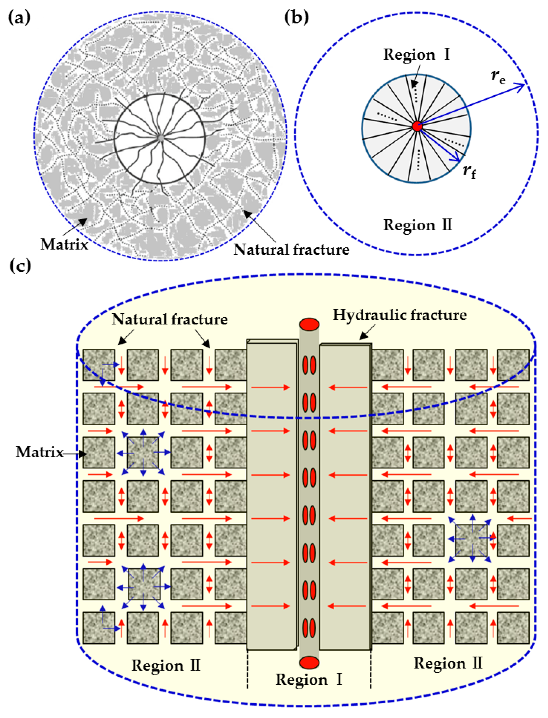
Figure 2.
Comparison results of the analytical and numerical solutions: (a) = 0.1, 10; (b) = 0.05, 0.5; (c) = 0.1, 0.001; (d) = 5 × 10⁻⁶, 5 × 10⁻⁴.
Figure 2.
Comparison results of the analytical and numerical solutions: (a) = 0.1, 10; (b) = 0.05, 0.5; (c) = 0.1, 0.001; (d) = 5 × 10⁻⁶, 5 × 10⁻⁴.
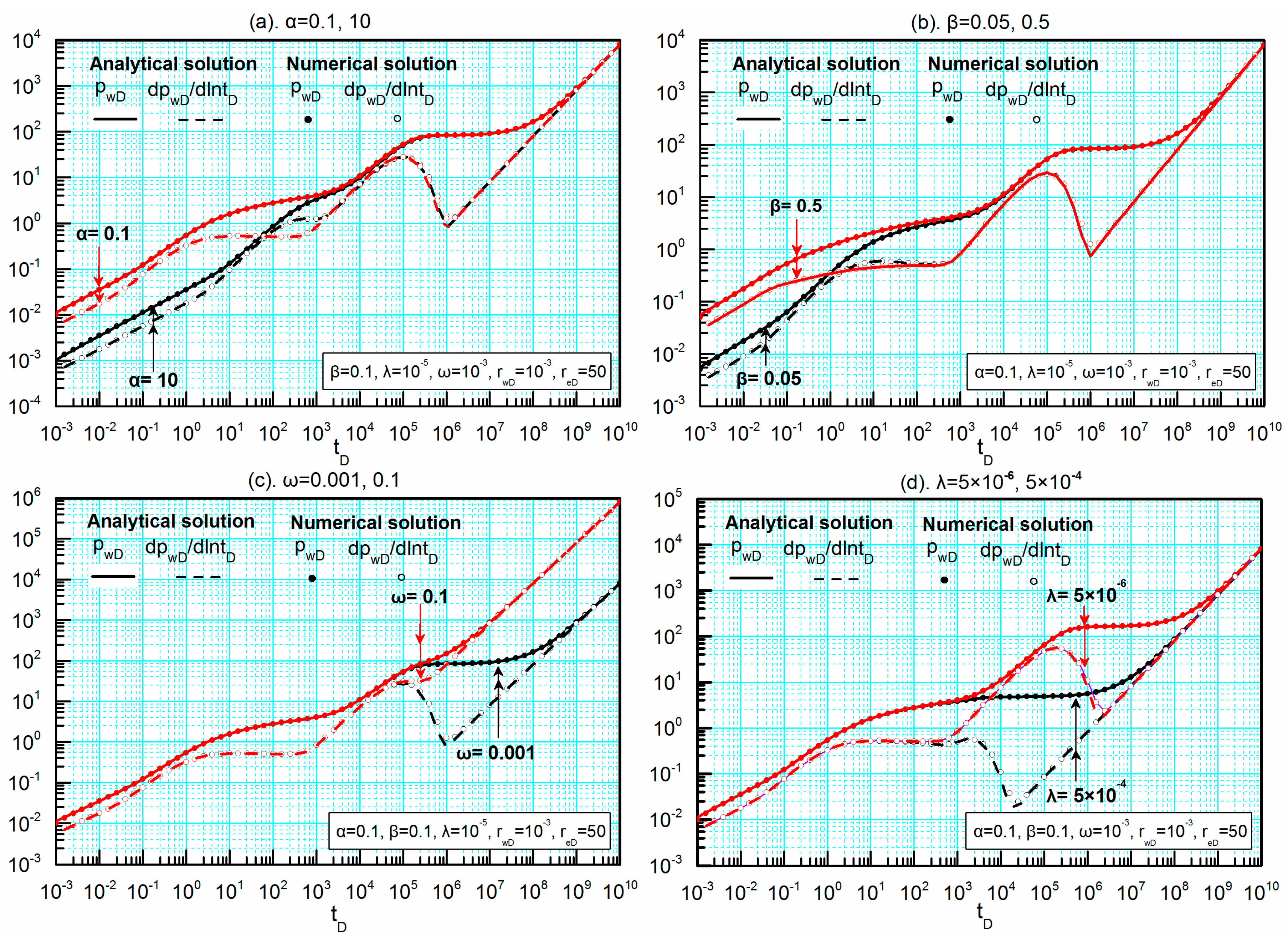
Figure 3.
The comparison of transient and cumulative rate curves between the models with and without volume fracturing.
Figure 3.
The comparison of transient and cumulative rate curves between the models with and without volume fracturing.

Figure 4.
Rate decline curves and cumulative rate curves for a volume fractured well at different values of interregional diffusivity ratio (α = 0.01, 0.1, 1 and 10).
Figure 4.
Rate decline curves and cumulative rate curves for a volume fractured well at different values of interregional diffusivity ratio (α = 0.01, 0.1, 1 and 10).

Figure 5.
Rate decline curves and cumulative rate curves for a volume fractured well at different values of interregional conductivity ratio (β = 0.01, 0.1, 1 and 10).
Figure 5.
Rate decline curves and cumulative rate curves for a volume fractured well at different values of interregional conductivity ratio (β = 0.01, 0.1, 1 and 10).

Figure 6.
Rate decline curves and cumulative rate curves for a volume fractured well at different values of fracture-matrix storativity ratio (ω = 10−3, 10−2, 10−1 and 0.9).
Figure 6.
Rate decline curves and cumulative rate curves for a volume fractured well at different values of fracture-matrix storativity ratio (ω = 10−3, 10−2, 10−1 and 0.9).

Figure 7.
Rate decline curves and cumulative rate curves for a volume fractured well at different values of fracture-matrix interporosity coefficient (λ = 10−6, 10−5, 10−4 and 10−3).
Figure 7.
Rate decline curves and cumulative rate curves for a volume fractured well at different values of fracture-matrix interporosity coefficient (λ = 10−6, 10−5, 10−4 and 10−3).
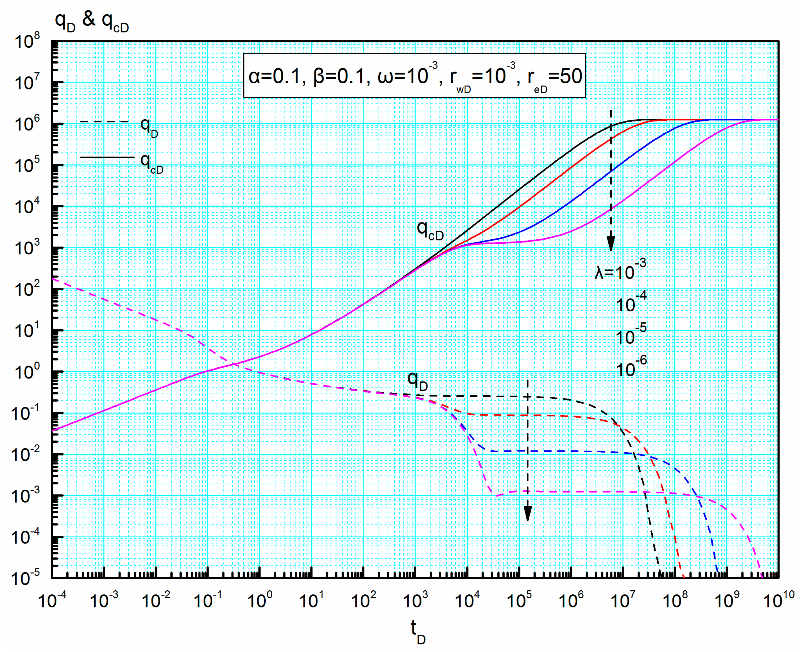
Figure 8.
Rate decline curves and cumulative rate curves for a volume fractured well at different values of dimensionless reservoir radius (reD = 50, 100, 200 and 400).
Figure 8.
Rate decline curves and cumulative rate curves for a volume fractured well at different values of dimensionless reservoir radius (reD = 50, 100, 200 and 400).
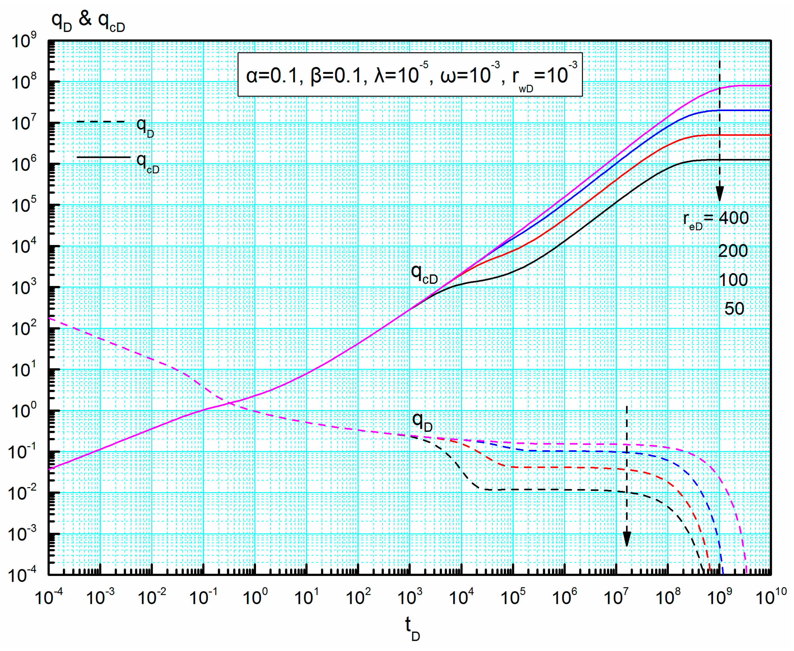
Figure 9.
Flow regimes on new Blasingame type curves for a volume fractured well in the naturally fractured reservoir (α = 0.1, β = 10, λ = 10−3, λ = 10−4, rwD = 0.001, reD = 0.1).
Figure 9.
Flow regimes on new Blasingame type curves for a volume fractured well in the naturally fractured reservoir (α = 0.1, β = 10, λ = 10−3, λ = 10−4, rwD = 0.001, reD = 0.1).
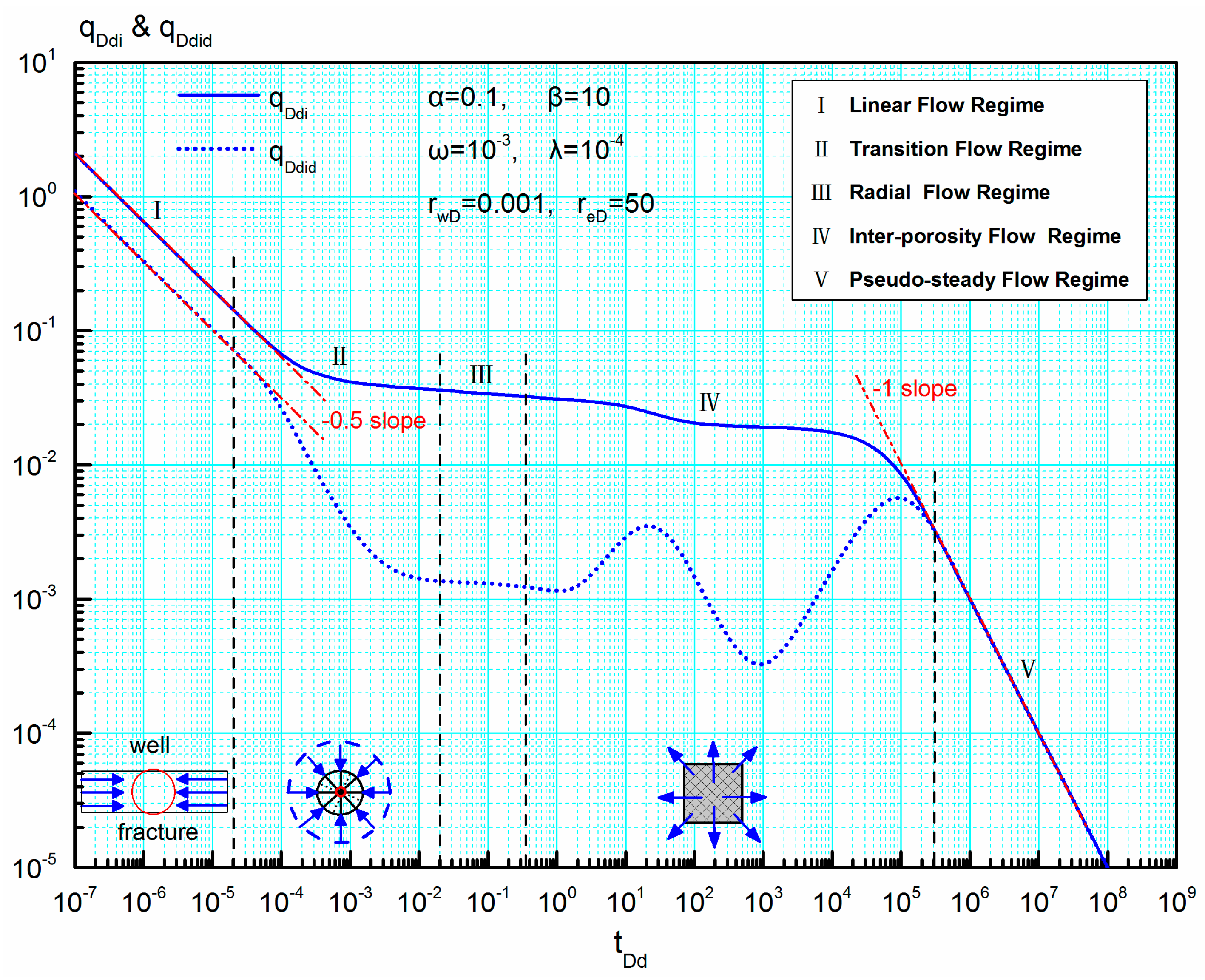
Figure 10.
New Blasingame type curves for a volume fractured well at different values of interregional diffusivity ratio (α = 0.01, 0.1, 1 and 10).
Figure 10.
New Blasingame type curves for a volume fractured well at different values of interregional diffusivity ratio (α = 0.01, 0.1, 1 and 10).
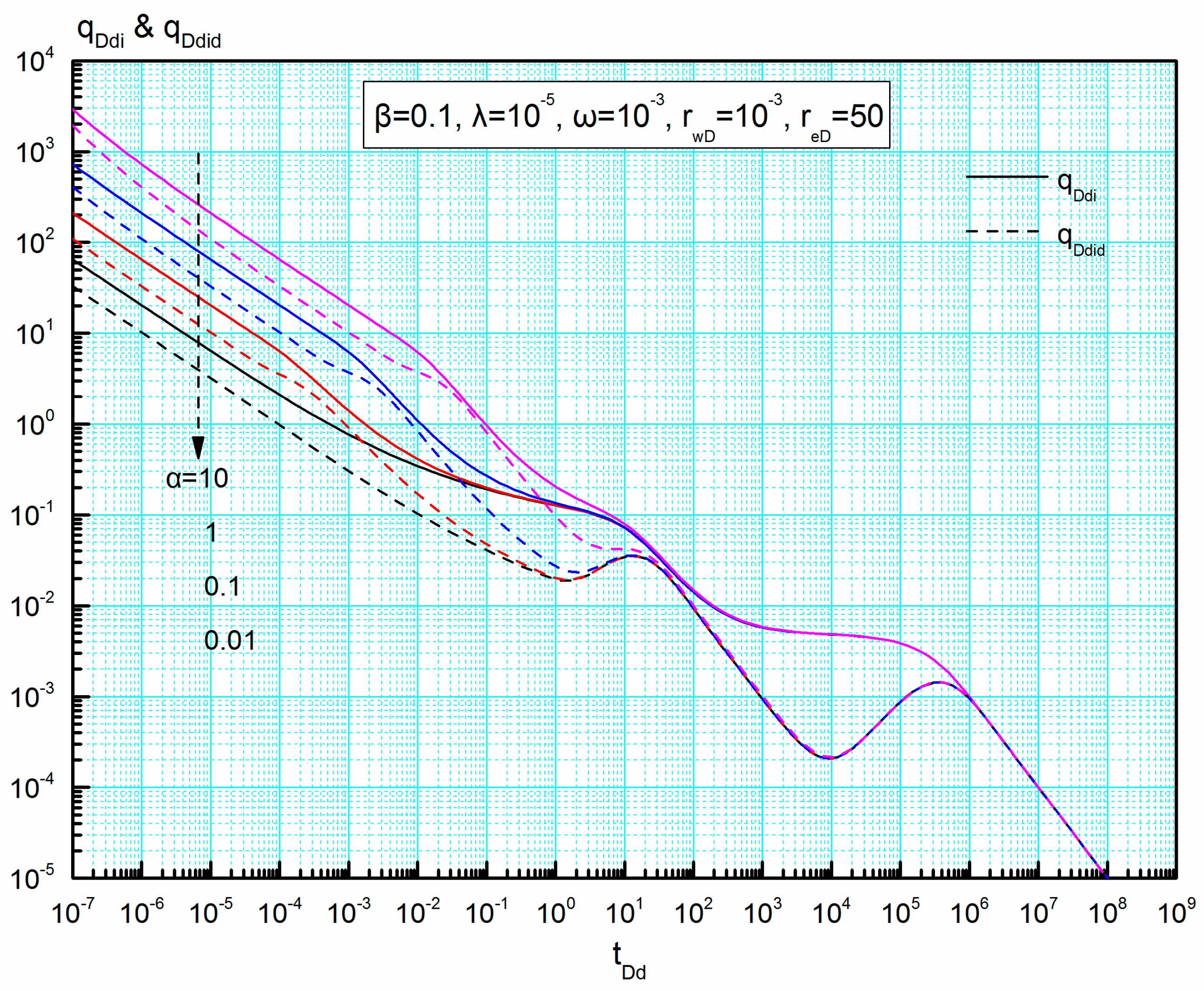
Figure 11.
New Blasingame type curves for a volume fractured well at different values of interregional conductivity ratio (β = 0.001, 0.01, 0.1 and 1).
Figure 11.
New Blasingame type curves for a volume fractured well at different values of interregional conductivity ratio (β = 0.001, 0.01, 0.1 and 1).
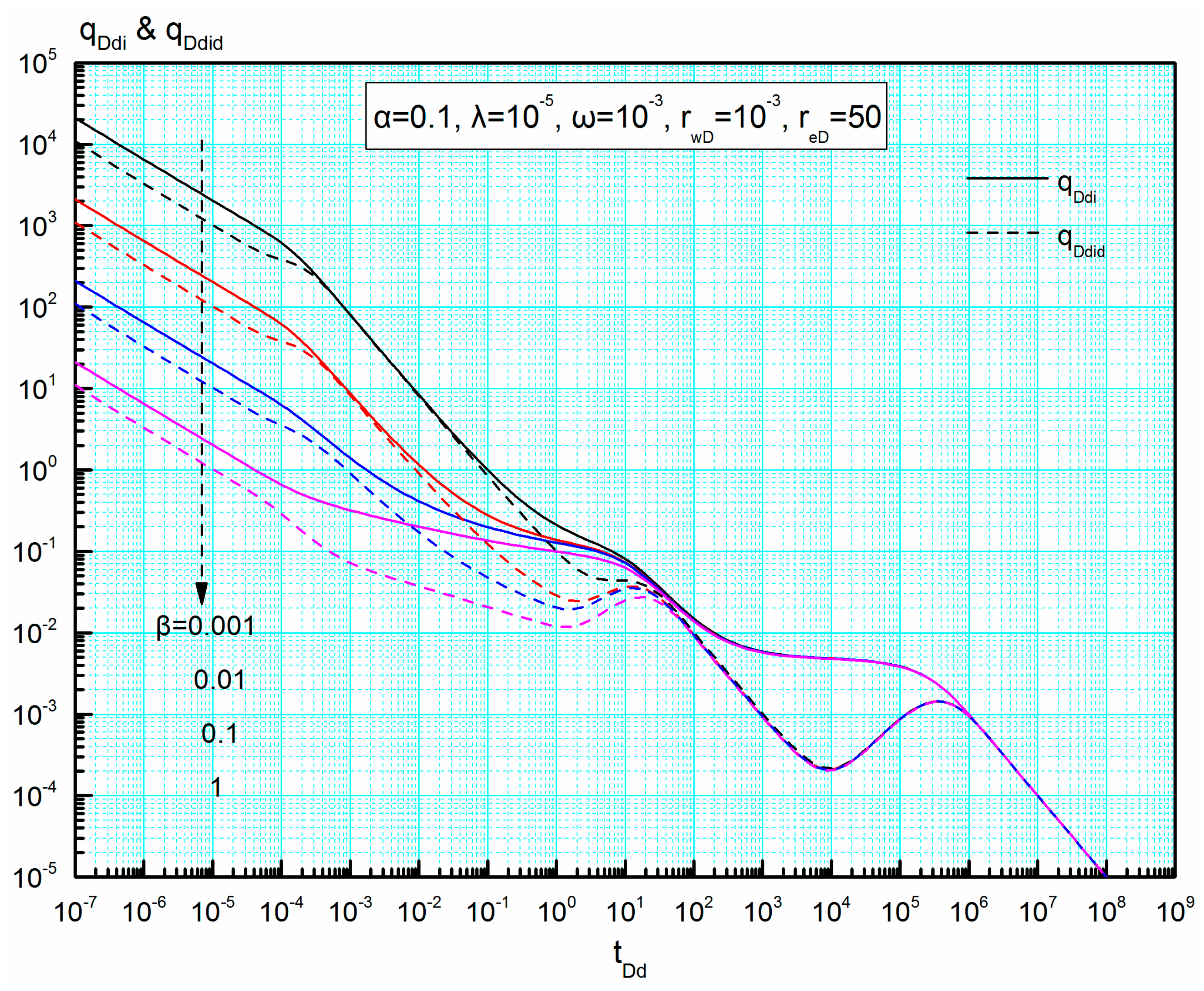
Figure 12.
New Blasingame type curves for a volume fractured well at different values of fracture-matrix storativity ratio (ω = 10−3, 10−2, 10−1 and 0.9).
Figure 12.
New Blasingame type curves for a volume fractured well at different values of fracture-matrix storativity ratio (ω = 10−3, 10−2, 10−1 and 0.9).

Figure 13.
New Blasingame type curves for a volume fractured well at different values of fracture-matrix interporosity coefficient (λ = 10−6, 10−5, 10−4 and 10−3).
Figure 13.
New Blasingame type curves for a volume fractured well at different values of fracture-matrix interporosity coefficient (λ = 10−6, 10−5, 10−4 and 10−3).
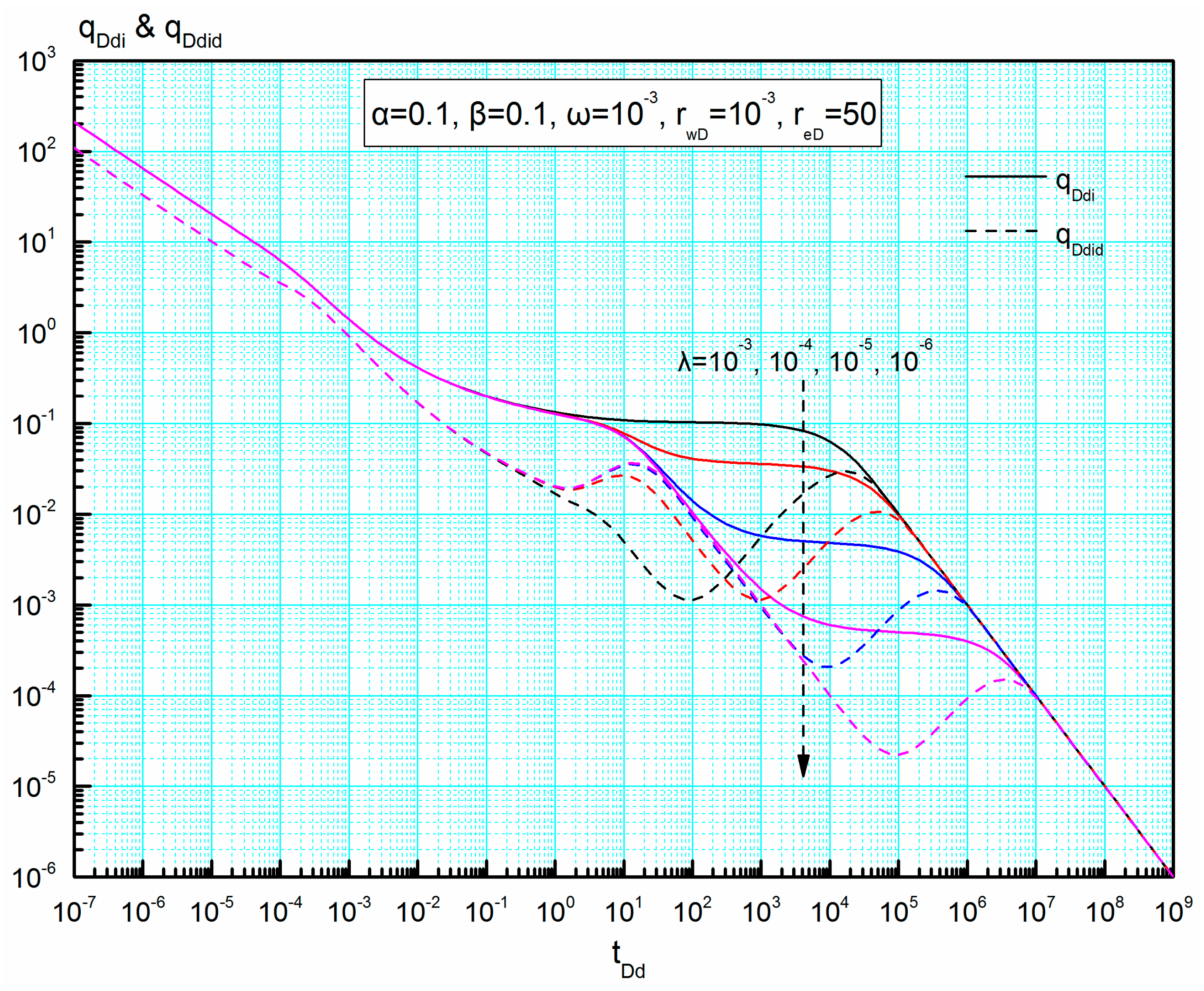
Figure 14.
New Blasingame type curves for a volume fractured well at different values of dimensionless reservoir radius (reD = 50, 100, 200 and 400).
Figure 14.
New Blasingame type curves for a volume fractured well at different values of dimensionless reservoir radius (reD = 50, 100, 200 and 400).
© 2018 by the authors. Licensee MDPI, Basel, Switzerland. This article is an open access article distributed under the terms and conditions of the Creative Commons Attribution (CC BY) license (http://creativecommons.org/licenses/by/4.0/).
Share and Cite
MDPI and ACS Style
Wang, M.; Fan, Z.; Xing, G.; Zhao, W.; Song, H.; Su, P. Rate Decline Analysis for Modeling Volume Fractured Well Production in Naturally Fractured Reservoirs. Energies 2018, 11, 43. https://doi.org/10.3390/en11010043
AMA Style
Wang M, Fan Z, Xing G, Zhao W, Song H, Su P. Rate Decline Analysis for Modeling Volume Fractured Well Production in Naturally Fractured Reservoirs. Energies. 2018; 11(1):43. https://doi.org/10.3390/en11010043
Chicago/Turabian StyleWang, Mingxian, Zifei Fan, Guoqiang Xing, Wenqi Zhao, Heng Song, and Penghui Su. 2018. "Rate Decline Analysis for Modeling Volume Fractured Well Production in Naturally Fractured Reservoirs" Energies 11, no. 1: 43. https://doi.org/10.3390/en11010043
Note that from the first issue of 2016, this journal uses article numbers instead of page numbers. See further details here.