Verification of Energy Reduction Effect through Control Optimization of Supply Air Temperature in VRF-OAP System

1
Department of Digital Appliances R&D Team, Samsung Electronics, 129, Samsung-ro, Yeongtong-gu, Suwon-si, Gyeonggi-do 16677, Korea
2
Building Technologies Research and Integration Center (BTRIC), Oak Ridge National Laboratory (ORNL), One Bethel Valley Road, Oak Ridge, TN 37831, USA
3
Department of Architectural Engineering, ERI, Gyeongsang National University, Jinju daero 501, Jinju City 52828, Korea
*
Author to whom correspondence should be addressed.
Energies 2018, 11(1), 49; https://doi.org/10.3390/en11010049
Submission received: 20 November 2017
/
Revised: 18 December 2017
/
Accepted: 21 December 2017
/
Published: 27 December 2017
Abstract
:This paper developed an algorithm that controls the supply air temperature in the variable refrigerant flow (VRF), outdoor air processing unit (OAP) system, according to indoor and outdoor temperature and humidity, and verified the effects after applying the algorithm to real buildings. The VRF-OAP system refers to a heating, ventilation, and air conditioning (HVAC) system to complement a ventilation function, which is not provided in the VRF system. It is a system that supplies air indoors by heat treatment of outdoor air through the OAP, as a number of indoor units and OAPs are connected to the outdoor unit in the VRF system simultaneously. This paper conducted experiments with regard to changes in efficiency and the cooling capabilities of each unit and system according to supply air temperature in the OAP using a multicalorimeter. Based on these results, an algorithm that controlled the temperature of the supply air in the OAP was developed considering indoor and outdoor temperatures and humidity. The algorithm was applied in the test building to verify the effects of energy reduction and the effects on indoor temperature and humidity. Loads were changed by adjusting the number of conditioned rooms to verify the effect of the algorithm according to various load conditions. In the field test results, the energy reduction effect was approximately 15–17% at a 100% load, and 4–20% at a 75% load. However, no significant effects were shown at a 50% load. The indoor temperature and humidity reached a comfortable level.
1. Introduction
The variable refrigerant flow (VRF) system was developed in Japan in 1982 [1], and entered the heating, ventilation, and air conditioning (HVAC) market in Europe in 1987 [2]. Currently, the VRF system market has expanded to China, South Korea, United States, Brazil, Turkey, and India. The market continues to grow, numbering 1.3 million units in 2014 and its market value has reached US $9.7 billion. The Building Services Research and Information Association (BSRIA) reported that the compound annual growth rate of the VRF system market from 2013 to 2018 will be 11%, and seems to show a substantial growth rate [3].
The VRF system consists of a single outdoor unit and multiple indoor units. The main components of the outdoor unit are a compressor and a condenser, and those of the indoor unit are evaporators and expansion valves. The outdoor unit and each of the indoor units are connected with the refrigerant pipe, and a refrigerant that is not harmful to the human body, such as R410a, is supplied to the indoor unit directly, thereby processing the indoor heat load at the heat exchanger inside the indoor unit. The VRF system varies the refrigerant flow rate using a variable speed compressor(s) in the outdoor unit, and the electronic expansion valves (EEVs) located in each indoor unit. The system meets the space cooling or heating load requirements by maintaining the zone air temperature at the set-point. The ability to control the refrigerant mass flow rate, according to the cooling and/or heating load enables the use of many indoor units with differing capacities in conjunction with one single outdoor unit. This unlocks the possibility of having individualized comfort control, simultaneous heating and cooling in different zones, and heat recovery from one zone to another. It may also lead to more efficient operations during part-load conditions [4]. However, regions where the VRF system has been adopted, including the USA, lack the recognition of the benefits of the energy efficiency in the VRF system. Furthermore, additional ventilation equipment is needed in existing VRF systems to complement the ventilation function, and various solutions need to be developed to overcome functional limitations of the VRF system, such as lack of solutions concerning optimal control and integration with other equipment [5,6].
Numerous researchers have studied the energy efficiency of the VRF system for many years. Several performance evaluation methods have been proposed for VRF systems: methods using performance indices, such as energy efficiency ratio (EER), coefficient of performance (COP), and seasonal energy efficiency ratio (SEER) [7,8], using the measured operational data in field tests [2,9], using simulation which is available to evaluate at the same boundary conditions, such as outdoor air condition and internal heating [10,11,12,13,14].The performance evaluations through the above methods reported that the VRF system had energy reduction effects of 40% to 60% compared to that of existing central HVAC systems, although there were some difference depending on operational method of the HVAC systems, buildings, and climate. In addition, studies have been conducted on solutions of efficient operation of the VRF system in actual buildings, in which refrigerant evaporation temperature (cooling) and high pressure (heating) were controlled according to load at partial load conditions, thereby reducing the needed energy while maintaining a comfortable indoor thermal environment [15,16].
The ventilation solutions in buildings where VRF systems were installed were as follows: Park et al. proposed energy recovery ventilation (ERV) and a dedicated outdoor air system (DOAS) [17], and Aynur et al. conducted evaluations on indoor thermal environments and energy consumption, while adopting the heat pump desiccant (HPD) [18,19,20]. Zhu et al. introduced a new combination of for HVAC system, as roof top unit (RTU) was used as the OAP in the VRF system, and proposed and evaluated control strategies, energy performance, thermal comfort, and indoor air quality (IAQ) for the system [21].
Im et al. [6] adopted the OAP as ventilation equipment for the VRF system. However, in contrast with the OAP, which had additional heat source equipment, including compressors, this study targeted an HVAC system that processed outdoor air loads by supplying refrigerants from the outdoor unit as an outdoor unit in the VRF system. This VRF system was connected to OAP along with multiple indoor units (hereafter referred to as VRF-OAP system) (Figure 1). In the VRF-OAP system, multiple indoor units and the OAP are connected to a single outdoor unit simultaneously. Thus, controlling the refrigerant flows is more difficult and important than that of the existing VRF system. Furthermore, outdoor air ingested by the OAP is air that is higher or lower in temperature than the indoor temperature. If the thermal load of the outdoor air is not completely processed and introduced to the indoor environment, negative impacts on the comfort of the indoor occupants is much greater than that of the indoor units that process the thermal loads of the indoor air. Because of this, the refrigerant flow control in the VRF-OAP system has been designed to have more flows to the OAP than to the indoor units, and most of the refrigerants inside the system are introduced to the OAP. Thus, the design guide suggests that the OAP capacity should be less than 30% of the outdoor unit capacity to prevent a lack of cooling and heating capacity in other connected indoor units. Im et al. compared the energy consumption and the indoor thermal environments at various partial load conditions with regard to the VRF-OAP system, a conventional roof top unit (RTU), and a variable air volume (VAV) system, thereby proving the superiority of the VRF-OAP system.
This paper developed a control algorithm of the supply air temperature in the OAP as a method to use the VRF-OAP system more efficiently in buildings. The control algorithm of the supply air temperature in the OAP refers to a control that increases the overall energy efficiency in the system, while maintaining a comfortable state in the indoor environment, by adjusting the refrigerant flow introduced to the OAP and the indoor unit appropriately through the supply air temperature control in the OAP, according to the indoor and outdoor temperature and humidity conditions during cooling operations. In this paper, changes in processing of sensible and latent heat in the VRF-OAP system and energy efficiency were investigated according to the supply air temperature through multicalorimeter experiments first, and then the control algorithm of the supply air temperature in the OAP was developed based on the investigation results. Furthermore, the algorithm was mounted to the VRF-OAP system installed in the test building to verify the algorithm effects in a real building.
2. Investigation of Cooling Capability and Efficiency According to Supply Air Temperature of OAP through Experiments
2.1. Experimental Method
The changes in the processing of sensible, latent heat, and changes in the energy efficiency ratio (EER) were measured according to the supply air temperature in the OAP of the VRF-OAP system using a multicalorimeter.
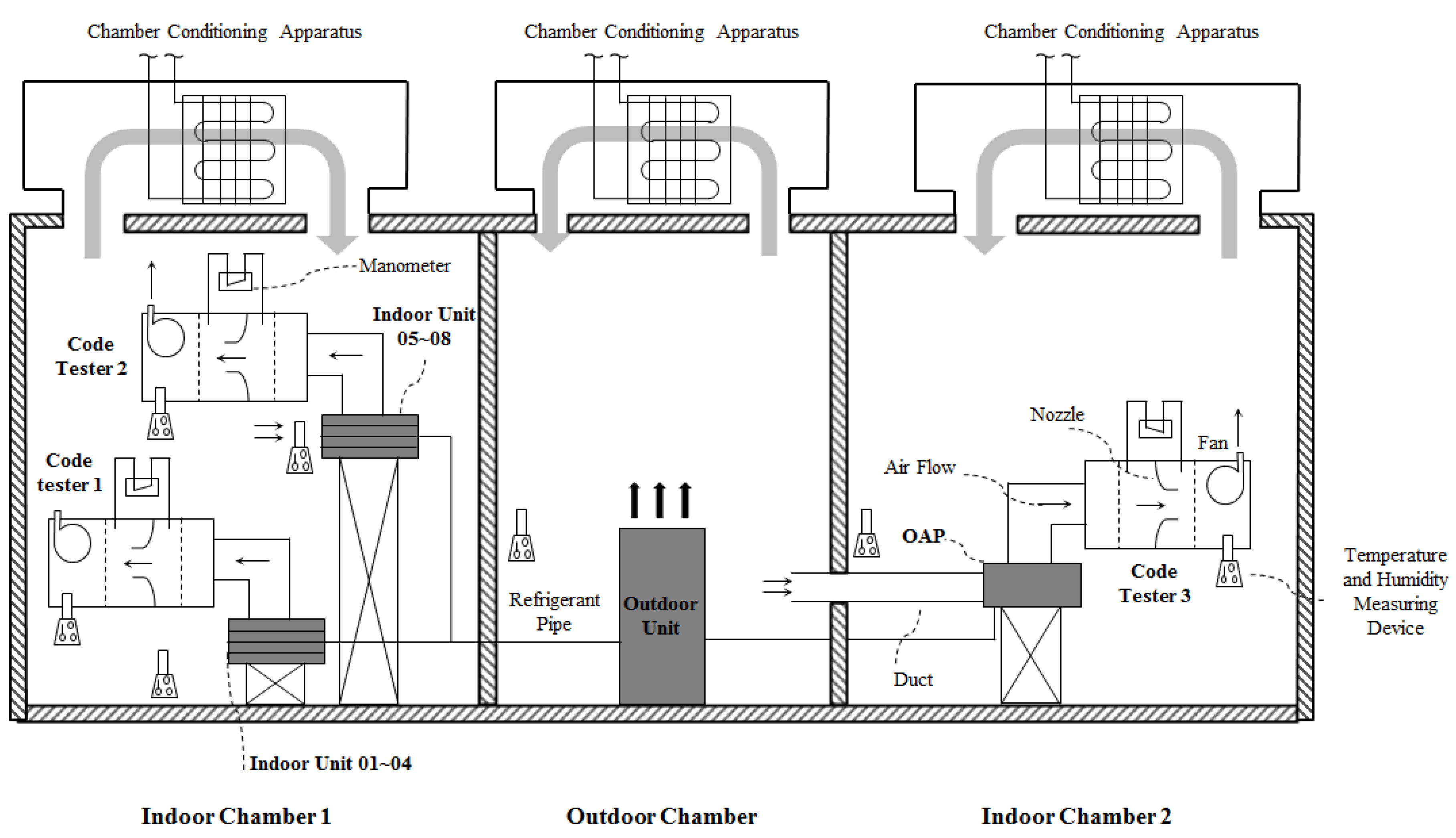
Figure 2 shows the configuration of the multicalorimeter and installation status of the VRF-OAP system. Table 1 and Table 2 present equipment specifications of the multicalorimeter and VRF-OAP system. The multicalorimeter consists of a single outdoor chamber that reproduces the outdoor air environment and two indoor chambers (indoor chamber 1, indoor chamber 2) that reproduces the indoor environments. In the outdoor chamber, there is one outdoor unit, and in the indoor chamber 1 and indoor chamber 2, eight indoor units and one OAP were installed. In addition, two code testers were installed in indoor chamber 1, and four indoor units were connected to each of the code testers. In indoor chamber 2, the OAP was connected to a single code tester. The indoor unit was installed to suck the air inside the indoor chamber directly, and OAP was installed to suck the air from the outdoor chamber through the duct. The cooling capacity that was controllable in the outdoor chamber was 14.5–145.3 kW, resulting in a range of air temperature that was −30–60 °C, and the range of relative humidity was 5–90%. Cooling capacities that were controllable in indoor chamber 1 and indoor chamber 2 were 5.8–58.1 kW, resulting in a range of air temperature that was 0–50 °C, and the range of relative humidity was 10–90%. Each of the chambers can maintain constant temperature and humidity control and satisfy a repeatability error of ±2%. The installed outdoor unit has 81.2 kW of cooling capacity and 8.79 kW of integrated cooling power input. The indoor unit has 7.2 kW of cooling capacity and 130 W of power input, and OAP has 22.4 kW of cooling capacity, and 300 W of power input. In addition, the temperature and humidity of air inside the chamber, the temperature and humidity of the air in the inlet and outlet of the indoor unit, the temperature and humidity of air in the inlet and outlet of the OAP, the air pressure difference inside the code tester, and the power consumption of all equipment was measured and monitored. The cooling capacities of the indoor unit and the OAP were calculated by the air enthalpy method, using the measured air temperature and humidity in the inlet and the outlet, the air pressure difference inside the code tester, and the cooling capacity of the outdoor unit. The cooling capacities of all indoor units and the OAP were summed.
Table 3 presents the test cases. Experiments were conducted with regard to the outdoor air temperatures of (DB/WB) 35 °C/24 °C, 32 °C/23 °C, and 30 °C/22 °C, and each of the outdoor air temperatures has the following supply air temperatures: 16 °C, 18 °C, 20 °C, and 24 °C. Note that the supply air temperatures were set to 16 °C, 18 °C, and 22 °C for the outdoor air temperature 30 °C. The indoor temperatures (DB/WB) were set to 27 °C/19 °C for all cases, and the air volume of the indoor unit and OAP were fixed to the rating value.
2.2. Experimental Results
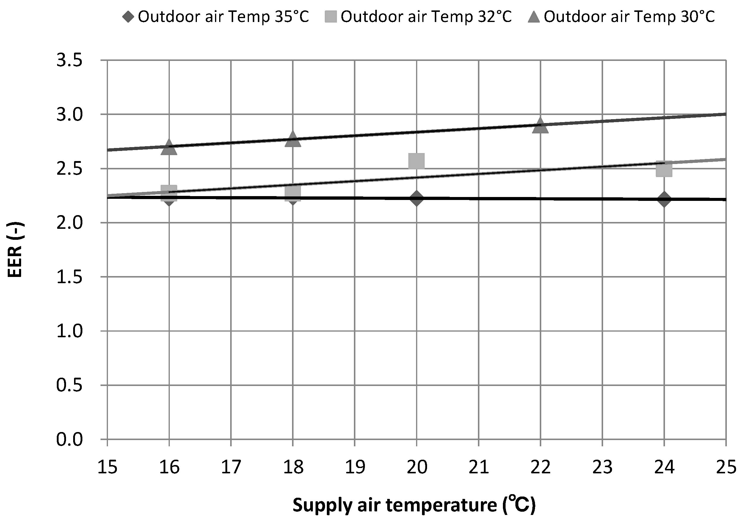
Operating data for 20 min, after the VRF-OAP system was run and the indoor unit and the OAP cooling capability reached a steady state, were measured and the experimental results were analyzed. A mean value of operating data was used in the analysis. Changes in cooling capacities of the indoor unit and the OAP according to the supply air temperature are presented in Table 4. The cooling capacities listed in the table refer to the sum of the processing amounts of sensible and latent heat. Since the experiments were conducted while maintaining the outdoor air temperature, which was the inlet air temperature, and the air volume was constant, the cooling capacity of the OAP was reduced as the supply air temperature was increased. On the contrary, the results verified that the cooling capacity of code tester 1 and code tester 2 that were connected to the indoor unit increased as the supply air temperature increased. The reason for the increased cooling capacity of the indoor unit was because of the refrigerant, which was supplied to the OAP previously, was now supplied to the indoor units, as the OAP capacity was reduced as the supply air temperature was increased. The overall cooling capacity in the VRF-OAP system was nearly the same at all supply air temperatures, notably in the all cases. The change in the latent heat processing amount according to the supply air temperatures (Figure 3) verified the rapid reduction in the latent heat processing amount above the dew point temperature (18.3 °C–19.4 °C) of the outdoor air conditions. Figure 4 shows the comparison results of the system EER according to the supply air temperature. The system EER is calculated by dividing the sum of the cooling capacities of the indoor units and OAP by calculating the power consumption of the outdoor units, the indoor units, and the OAP. The comparison results showed that although a change in the system EER was not revealed at 35 °C according to the supply air temperature, the EER was improved at 32 °C and 30 °C outdoor air temperature as the supply air temperature was increased. When the supply air temperature was set to 24 °C, the EER improved by about 11.1% at an outdoor air temperature of 32 °C and by about 9.3% at an outdoor air temperature of 30 °C, as compared to that at the 16 °C supply air temperature.
3. Development of Supply Air Temperature Control Algorithm for VRF-OAP System
The results of the multicalorimeter experiment verified that the system efficiency was improved as the supply air temperature in the VRF-OAP system was increased. In addition, the reduction in overall cooling capacity in the system was not exhibited according to the supply air temperature, which indicated that there would be no significant effect on the indoor temperature through the control of the supply air temperature. However, when the supply air temperature was higher than the dew point temperature of the outdoor air, it would cause an increase in the indoor humidity as a result of the reduction in the latent heat processing amount. Thus, this study developed a control algorithm for the supply air temperature that improved the overall efficiency of the system by setting the supply air temperature as much as possible, while maintaining the indoor relative humidity within the range of comfort.
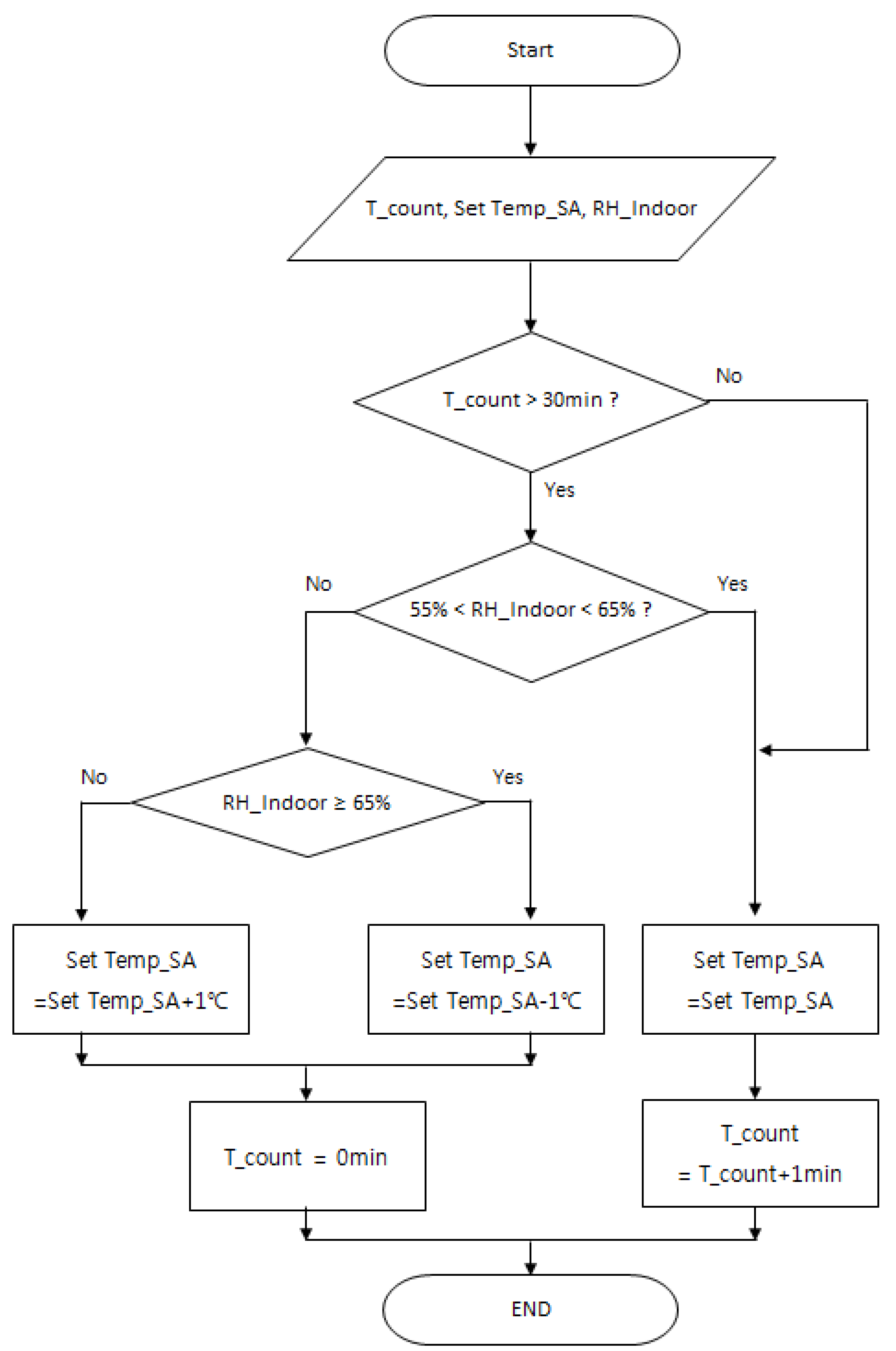
Figure 5 shows the flow chart of the control algorithm. The input data in the control algorithm were the elapsed time (T_count) after changing the supply air temperature, the current set value of the supply air temperature (Set Temp_SA), and the indoor relative humidity (RH_indoor). A control range of the supply air temperature was 13–24 °C, and the initial set value was 18 °C. First, whether the T_count exceeded 30 min. was determined. If it did not exceed 30 min, the current set value of the supply air temperature was maintained and one min was added to the T_count followed by termination. If the T_count exceeded 30 min, Set Temp_SA was determined according to the RH_indoor. Here, 30 min. of the T_count was determined considering the time for the supply air temperature to reach the set value after changing the set value of the supply air temperature and a waiting time of for an improvement of the system efficiency due to the change in the supply air temperature. If RH_indoor was within 60 ± 5%, which was a comfort range, Set Temp_SA was maintained without change, if it was above 65%, “Set Temp_SA was lowered by 1 °C”, and if it was below 55%, “Set Temp_SA was raised by 1 °C” was applied. If Set Temp_SA was changed, the T_count was reset to 0 min, and if it was maintained, one min. was added to the T_count and the algorithm terminated. The control algorithm was run continuously once every min.
4. Verification of the Control Algorithm Effect through Building Application
4.1. Target Building and HVAC System
The test building is a two-story, 3200 ft2 (297.3 m2) multi-zone unoccupied building that represents a typical low-rise, small office building common in the US existing building stock (Figure 6) [6]. The occupancy of the building can be simulated by the control of the lighting and other internal loads. In addition, a dedicated weather station is installed on the roof that provides actual weather data for use in performance analysis. The building is equipped with a 12-ton (42 kW) VRF-OAP system. Table 5 summarizes the building and system characteristics.
Figure 7 shows a schematic of the VRF-OAP system used for the test building. The VRF system has a 12 ton (42 kW) outdoor unit, one OAP unit, and ten indoor units with capacities ranging from 0.5–1.5 ton (1.8–5.3 kW). The ten indoor units and the OAP are connected to the same VRF outdoor unit, and the OAP provides the conditioned outdoor air to ten zones at 0.189 m3/s (400 CFM) [9,22]. An exhaust fan is located on each floor and operates continuously. The air-side monitoring points included the room temperature and relative humidity, supply and return air temperatures and relative humidity. Power consumptions for the VRF outdoor unit, each VRF indoor unit, and the OAP were measured as well.
4.2. Verification of the OAP Control Algorithm Effect through Field Tests
4.2.1. Field Test Method
The use schedule of buildings is categorized into occupied and unoccupied hours. The operational schedule of internal loads and the operation method of HVAC system are determined by those hours. The occupied hours of the building are from 6:00 to 18:00. At all other times, the building is unoccupied. The HVAC systems including the ventilation equipment were continually operated. The room temperature was set at 24 °C for cooling. During unoccupied hours, the room temperature was set at 30 °C. Room humidity was not controlled. The test building is an unoccupied research facility, where occupancy will be simulated by controlling lighting and other internal loads to minimize human interference with the building, which is one of the main factors for uncertainty in building energy use. The internal loads are estimated and simulated using portable heaters and humidifiers with preprogrammed timers. The capacity and operational schedule of portable heaters and humidifiers is defined according to the ASHRAE Standard 90.1–1989.
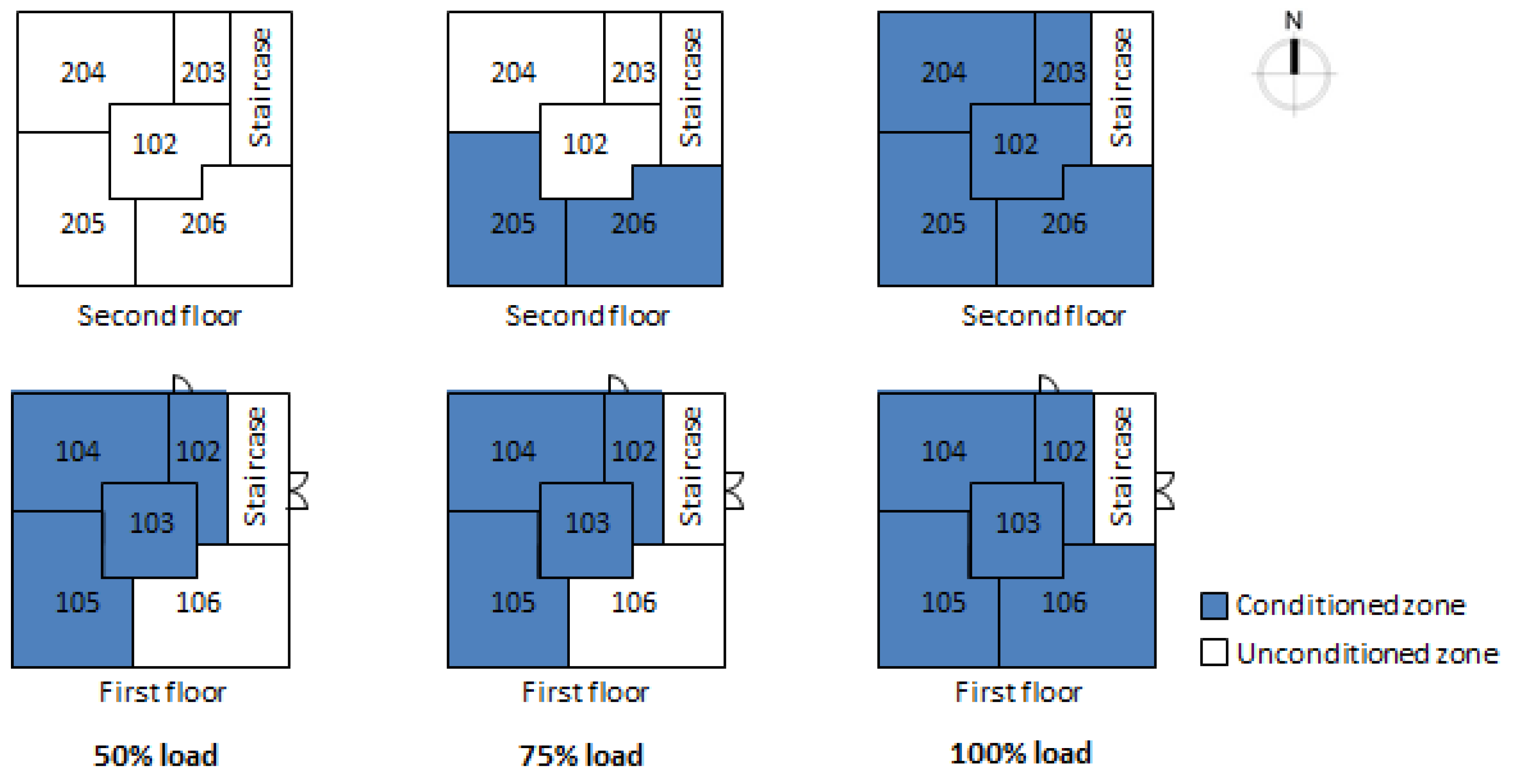
A load was changed by adjusting the number of conditioned rooms to verify the effect of the control of the supply air temperature in various load conditions. Figure 8 illustrates the scheme of operations to emulate (a) 50% load, (b) 75% load, and (c) 100% load. Each system was operated alternately for eight days for three days each for 50% and 75% loads and for two days for a 100% load. Table 6 shows the field test schedule. Here, conventional control refers to a baseline to calculate the effect of the control of supply air temperature. It is an operation that maintains the supply air temperature at 18 °C constantly. In addition, the algorithm refers to an operation where the developed of the control algorithm of the supply air temperature is applied.
4.2.2. Field Test Results
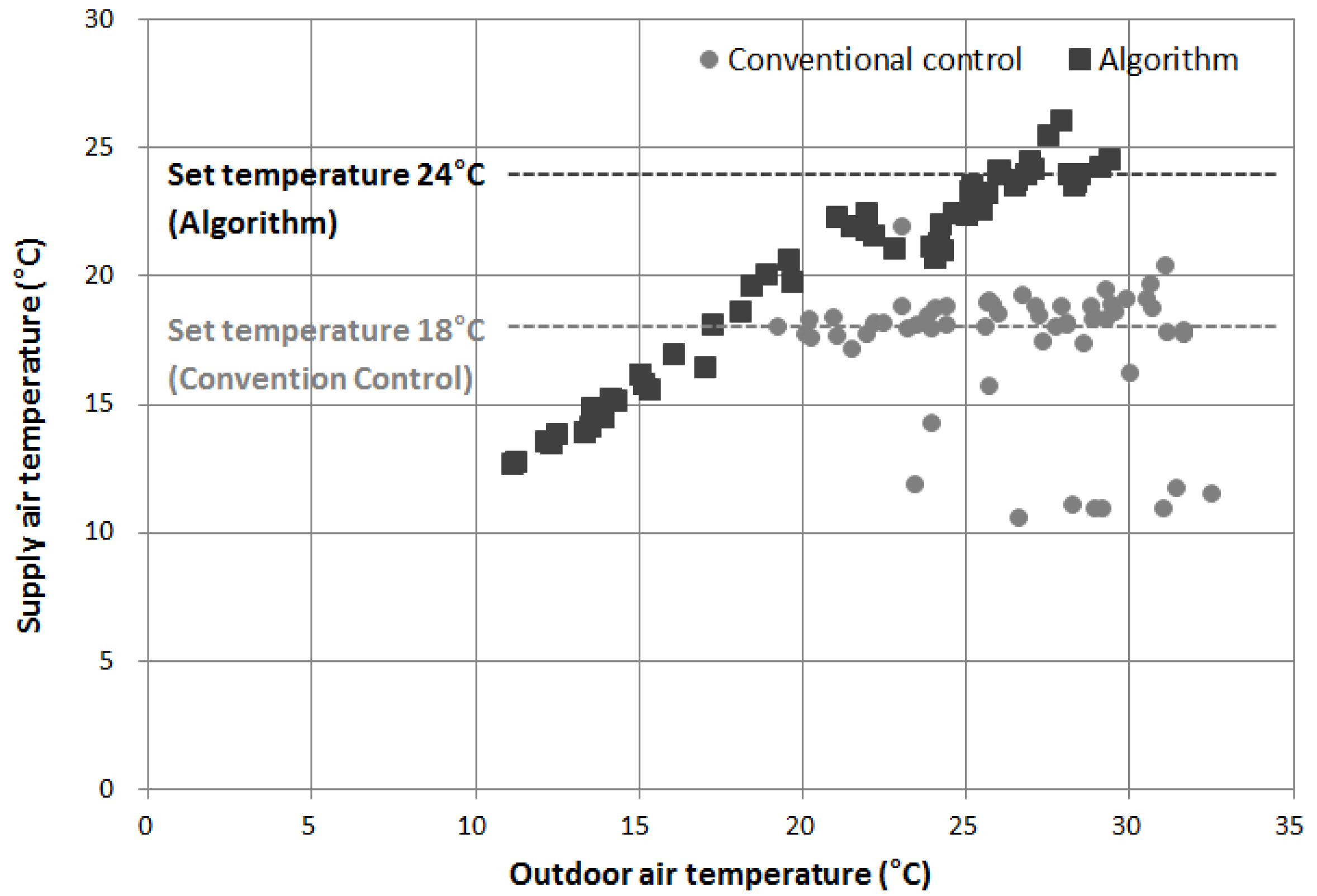
To verify the effects of the control algorithm of the supply air temperature in the OAP, operation data during only occupied hours were used. The supply air temperature when conventional controls and the algorithm were applied is shown in Figure 9 as a form of a correlation graph with outdoor air temperature. For outdoor and supply air temperatures, one-hour mean values were used. The supply air temperature in the conventional control was controlled to a set value 18 °C, regardless of the outdoor air temperature at most of the times. The set value of the supply air temperature in the algorithm operation was 24 °C at all times during the measurement period. The supply air temperature was controlled and set to the value of 24 °C when the outdoor air temperature was higher than 24 °C, and the ingested outdoor air was supplied to the indoor directly in the section where the outdoor air temperature was lower than 24 °C.
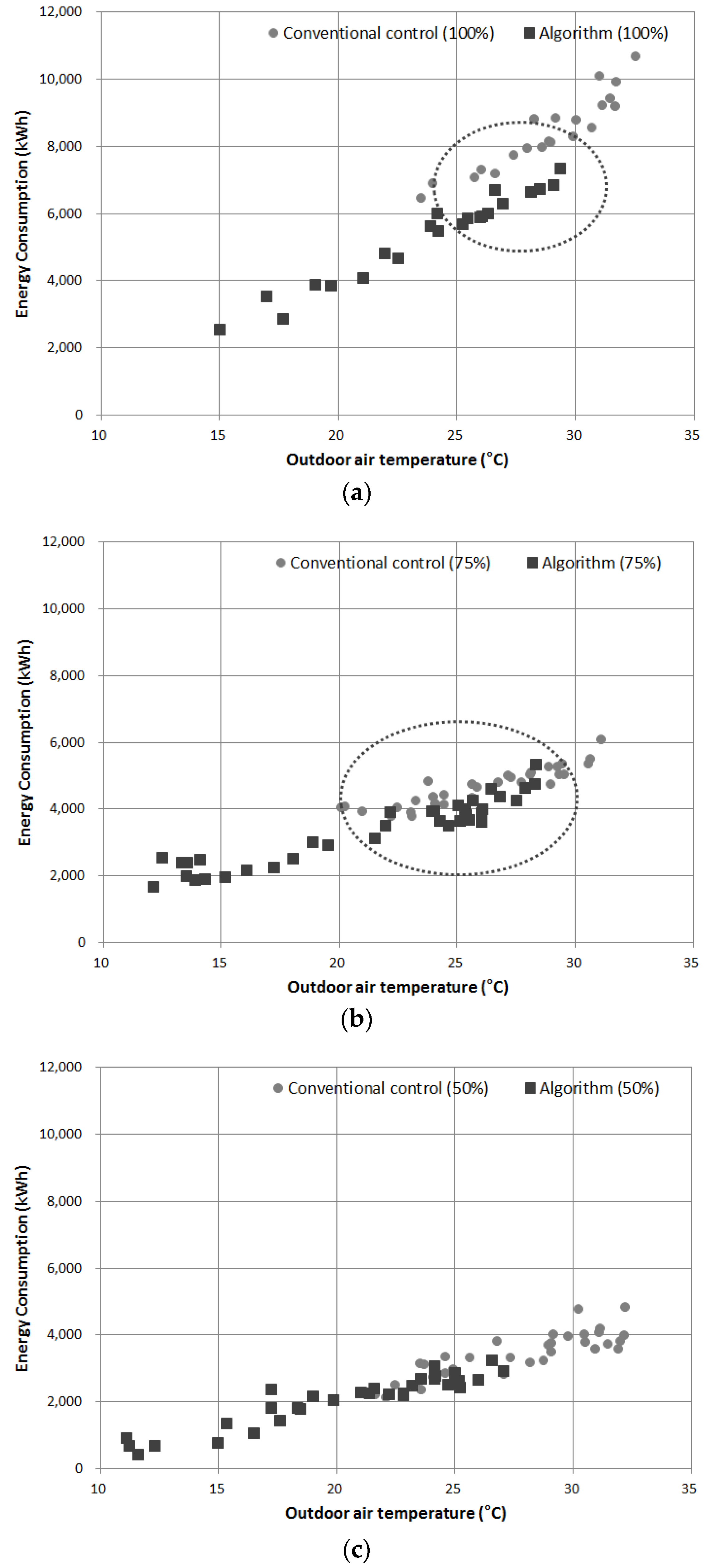
Next, the analysis results of changes in energy consumption according to the outdoor air temperature are shown in Figure 10. The conventional control and the algorithm-applied periods were July and September, which were different demonstration periods. Thus, a difference in the distribution of outdoor air temperature occurred, and the energy reduction effects of the algorithm were analyzed only for the section where the outdoor air temperature distribution for each load overlapped. As a result, the energy consumption during the algorithm application was reduced significantly at a 100% load compared to that of the conventional control, whereas a slight reduction effect was revealed at a 75% load. On the contrary, energy consumptions under each control at s 50% load were revealed to be similar. A regression analysis was conducted with the results at 100% and 75% loads in order to determine the algorithm control effect more quantitatively. In the regression analysis, operation data at a 25–30 °C outdoor air temperature at a 100% load and operation data of an outdoor temperature of 20–30 °C at a 75% load were employed. The regression analysis results are expressed in Equations (1)–(4). R2 value of each regression analysis is as follows: Equation (1) is 0.70, Equation (2) is 0.85, Equation (3) is 0.78, and Equation (4) is 0.62. The energy consumption and energy reduction rate by load according to the outdoor air temperature through the regression equations are presented in Table 7. A large energy reduction effect of 15–17% was exhibited at a 100% load. The highest energy reduction effect was revealed as 20% at the outdoor air temperature of 20 °C at a 75% load. The energy reduction effect was decreased as the outdoor air temperature increased, resulting in only a 4.6% energy reduction effect at an outdoor temperature of 30 °C. The above results indicate that the control algorithm of the supply air temperature was more effective with higher loads, and the reduction effects became larger as the outdoor air temperature became lower under the same load conditions.
PCon_100% = 370.689 × Toa − 2422.585 (R2 = 0.70)
PAl_100% = 332.375 × Toa − 2618.448 (R2 = 0.85)
PCon_75% = 157.305 × Toa + 523.574 (R2 = 0.78)
PAl_75% = 206.597 × Toa − 1194.737 (R2 = 0.62)
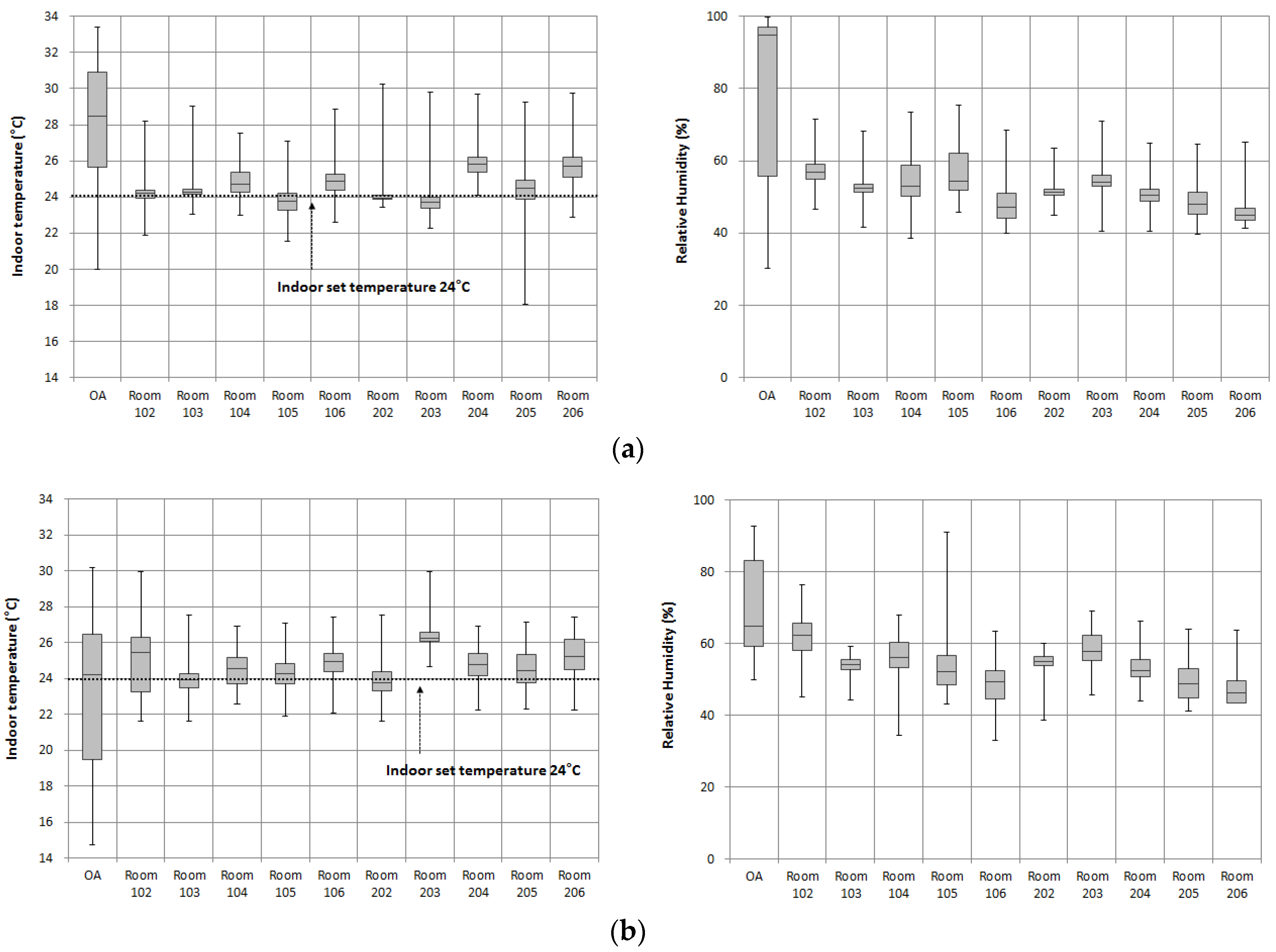
Figure 11 shows the analysis results of indoor temperature and indoor relative humidity. The indoor mean temperature of all rooms was similar under conventional (24.6 °C) and algorithm controls (24.7 °C) as well as room temperature distribution, hence verifying that both controls worked well according to the set temperature. The indoor mean relative humidity of all rooms was also similar under conventional (51.7%) and algorithm controls (53.6%), and the comfort range for the relative humidity was well controlled without exceeding 60 ± 5% used in the algorithm.
5. Conclusions
This paper developed the control algorithm for the supply air temperature in the OAP for VRF-OAP systems, and verified the effects by applying the algorithm to a test building. To develop the control algorithm, the cooling capability of the VRF-OAP system and changes in efficiency according to the supply air temperature were experimented using a multicalorimeter. With the increase in the supply air temperature, the cooling capacity of the OAP was decreased, but the overall cooling capability in the system was nearly the same, as the cooling capability of the indoor unit increased. This study result verified that the latent heat processing amount rapidly decreased at a supply air temperature which was higher than the dew point temperature of the outdoor air. The system EER was improved at outdoor air temperatures of 32 °C and 30 °C as the supply air temperature increased, resulting in about 11% at an outdoor air temperature of 32 °C and approximately a 9% improvement at an outdoor temperature of 30 °C; the supply air temperature was set to 24 °C compared to the system EER at 16 °C. Based on the above results, the control algorithm that improved system efficiency was developed by raising the supply air temperature as much as possible within a range where the indoor relative humidity did not affect the comfort of occupants. The algorithm was mounted on the test building, in which the indoor load was controlled by portable heaters and humidifiers and the effects of the algorithm were verified under various load conditions (100% load, 75% load, and 50% load). The field test results exhibited the effects of energy reduction are higher at 100% load than 75% load at the same temperature. At the same load, higher reduction effects were revealed when the outdoor air temperature was lower. However, this field test did not collect sufficient data to verify the algorithm effects, as the demonstration period was too short for each control. For future studies, the algorithm effects should be verified through a long-term demonstration period.
Acknowledgments
This work was supported by the National Research Foundation of Korea (NRF) grant funded by the Korea government (MSIP) (No. 2017R1A2B2006424). This manuscript has been authored by UT-Battelle, LLC, under Contract Number DE-AC05-00OR22725 with the U.S. Department of Energy. The United States Government retains and the publisher, by accepting the article for publication, acknowledges that the United States Government retains a non-exclusive, paid-up, irrevocable, world-wide license to publish or reproduce the published form of this manuscript, or allow others to do so, for United States Government purposes.
Author Contributions
J.H.L. conceived and designed the experiments; H.J.Y. and P.I. performed the experiments; J.H.L. and Y.-h.S. analyzed the data; H.J.Y. and P.I. contributed reagents/materials/analysis tools; J.H.L. and Y.-h.S. wrote the paper.
Conflicts of Interest
The authors declare no conflict of interest.
Disclaimer
This effort was supported by Samsung Electronics and the U.S. Department of Energy. Neither the United States Government nor any agency thereof, nor any of their employees, makes any warranty, express or implied, or assumes any legal liability or responsibility for the accuracy, completeness, or usefulness of any information, apparatus, product, or process disclosed, or represents that its use would not infringe upon privately owned rights. Reference herein to any specific commercial product, process, or service by trade name, trademark, manufacturer, or otherwise, does not necessarily constitute or imply its endorsement, recommendation, or favoring by the United States Government or any agency thereof. The views and opinions of the authors expressed herein do not necessarily state or reflect those of the United States Government or any agency thereof.
References
- Thornton, B.; Wagner, A. Variable Refrigerant Flow Systems; Prepared for the General Services Administration; Pacific Northwest National Laboratory: Richland, WA, USA, 2012. [Google Scholar]
- Goetzler, W. Variable Refrigerant Flow Systems. ASHRAE J. 2007, 49, 24–31. [Google Scholar]
- BSRIA. World Air Conditioning Market Grows Thanks to Hot Spots. May 2015. Available online: https://www.bsria.co.uk/news/article/world-air-conditioning-market-grows-thanks-to-hot-spots/ (accessed on 26 December 2017).
- Big Ladder Software, Engineering Reference—EnergyPlus 8.6. Available online: http://bigladdersoftware.com/epx/docs/8-6/engineering-reference/variable-refrigerant-flow-heat-pumps.html#variable-refrigerant-flow-heat-pump-model-system-curve-based-model (accessed on 26 December 2017).
- Alahmer, A.; Alsaqoor, S. Simulation and optimization of multi-split variable refrigerant flow systems. Ain Shams Eng. J. 2017, in press. [Google Scholar] [CrossRef]
- Im, P.; Malhotra, M.; Munk, J.D.; Lee, J. Cooling Season Full and Part Load Performance Evaluation of Variable Refrigerant Flow (VRF) System Using an Occupancy Simulated Research Building. In Proceedings of the 16th International Refrigeration and Air Conditioning Conference at Purdue, West Lafayette, IN, USA, 11–14 July 2016. [Google Scholar]
- 2010 Standard for Performance Rating of Variable Refrigerant Flow (VRF) Multi-Split Air-Conditioning and Heat Pump Equipment; ANSI/AHRI Standard 1230 with Addendum1; ANSI/AHRI: Arlington, VA, USA, 2010.
- Air Conditioners, Liquid Chilling Packages and Heat Pumps, with Electrically Driven Compressors, for Space Heating and Cooling—Testing and Rating at Part Load Conditions and Calculation of Seasonal Performance; BS EN 14825:2016; BSI Standards: London, UK, 2016.
- Southard, L.E.; Liu, X.; Spitler, J.D. Performance of HVAC Systems at ASHRAE HQ. ASHRAE J. 2014, 56, 14. [Google Scholar]
- Zhou, Y.P.; Wu, J.Y.; Wang, R.Z.; Shiochi, S. Energy simulation in the variable refrigerant flow air-conditioning system under cooling conditions. Energy Build. 2007, 39, 212–220. [Google Scholar] [CrossRef]
- Li, Y.; Wu, J.; Shiochi, S. Modeling and energy simulation of the variable refrigerant flow air conditioning system with water-cooled condenser under cooling conditions. Energy Build. 2009, 41, 949–957. [Google Scholar] [CrossRef]
- Aynur, T.N.; Hwang, Y.; Radermacher, R. Simulation comparison of VAV and VRF air conditioning systems in an existing building for the cooling season. Energy Build. 2009, 41, 1143–1150. [Google Scholar] [CrossRef]
- Yun, G.Y.; Choi, J.; Kim, J.T. Energy performance of direct expansion air handling unit in office buildings. Energy Build. 2014, 77, 425–431. [Google Scholar] [CrossRef]
- Kim, D.; Cox, S.J.; Cho, H.; Im, P. Evaluation of energy savings potential of variable refrigerant flow (VRF) from variable air volume (VAV) in the U.S. climate locations. Energy Rep. 2017, 3, 85–93. [Google Scholar] [CrossRef]
- Yun, G.Y.; Lee, J.H.; Kim, H.J. Development and application of the load responsive control of the evaporating temperature in a VRF system for cooling energy savings. Energy Build. 2016, 116, 638–645. [Google Scholar] [CrossRef]
- Yun, G.Y.; Lee, J.H.; Kim, I. Dynamic target high pressure control of a VRF system for heating energy savings. Appl. Therm. Eng. 2017, 113, 1386–1395. [Google Scholar] [CrossRef]
- Park, D.Y.; Yun, G.; Kim, K.S. Experimental evaluation and simulation of a variable refrigerant-flow (VRF) air-conditioning system with outdoor air processing unit. Energy Build. 2017, 146, 122–140. [Google Scholar] [CrossRef]
- Aynur, T.N.; Hwang, Y.; Radermacher, R. Field performance measurements of a heat hump desiccant unit in dehumidification mode. Energy Build. 2008, 40, 2141–2147. [Google Scholar] [CrossRef]
- Aynur, T.N.; Hwang, Y.; Radermacher, R. Integration of variable refrigerant flow and heat pump desiccant systems for the cooling season. Appl. Therm. Eng. 2010, 30, 917–927. [Google Scholar] [CrossRef]
- Aynur, T.N.; Hwang, Y.; Radermacher, R. Integration of variable refrigerant flow and heat pump desiccant systems for the heating season. Energy Build. 2010, 42, 468–476. [Google Scholar] [CrossRef]
- Zhu, Y.; Jin, X.; Du, Z.; Fang, X.; Fan, B. Control and energy simulation of variable refrigerant flow air conditioning system combined with outdoor air processing unit. Appl. Therm. Eng. 2014, 64, 385–395. [Google Scholar] [CrossRef]
- ASHRAE. Thermal Environmental Conditions for Human Occupancy; ANSI/ASHRAE Standard 55–2013; American Society of Heating, Refrigeration and Air-Conditioning Engineers: Atlanta, GA, USA, 2013. [Google Scholar]
Figure 1.
Schematic of OAP system. (a) Conventional OAP system; (b) Target VRF-OAP system.

Figure 2.
Configuration of the multicalorimeter and installation status of the VRF-OAP system.

Figure 3.
Changes in latent heat processing amount in the OAP according to supply air temperature.
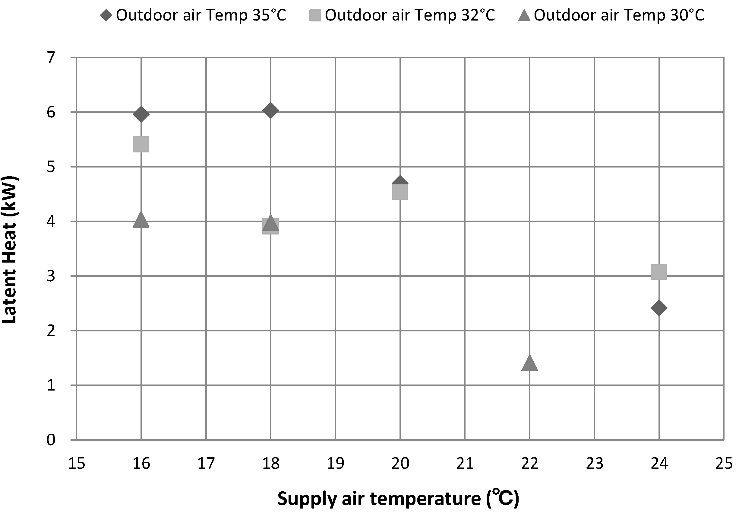
Figure 4.
Changes in the system EER according to supply air temperature.

Figure 5.
Flow chart of the control algorithm of supply air temperature in the OAP.

Figure 6.
Test Building.
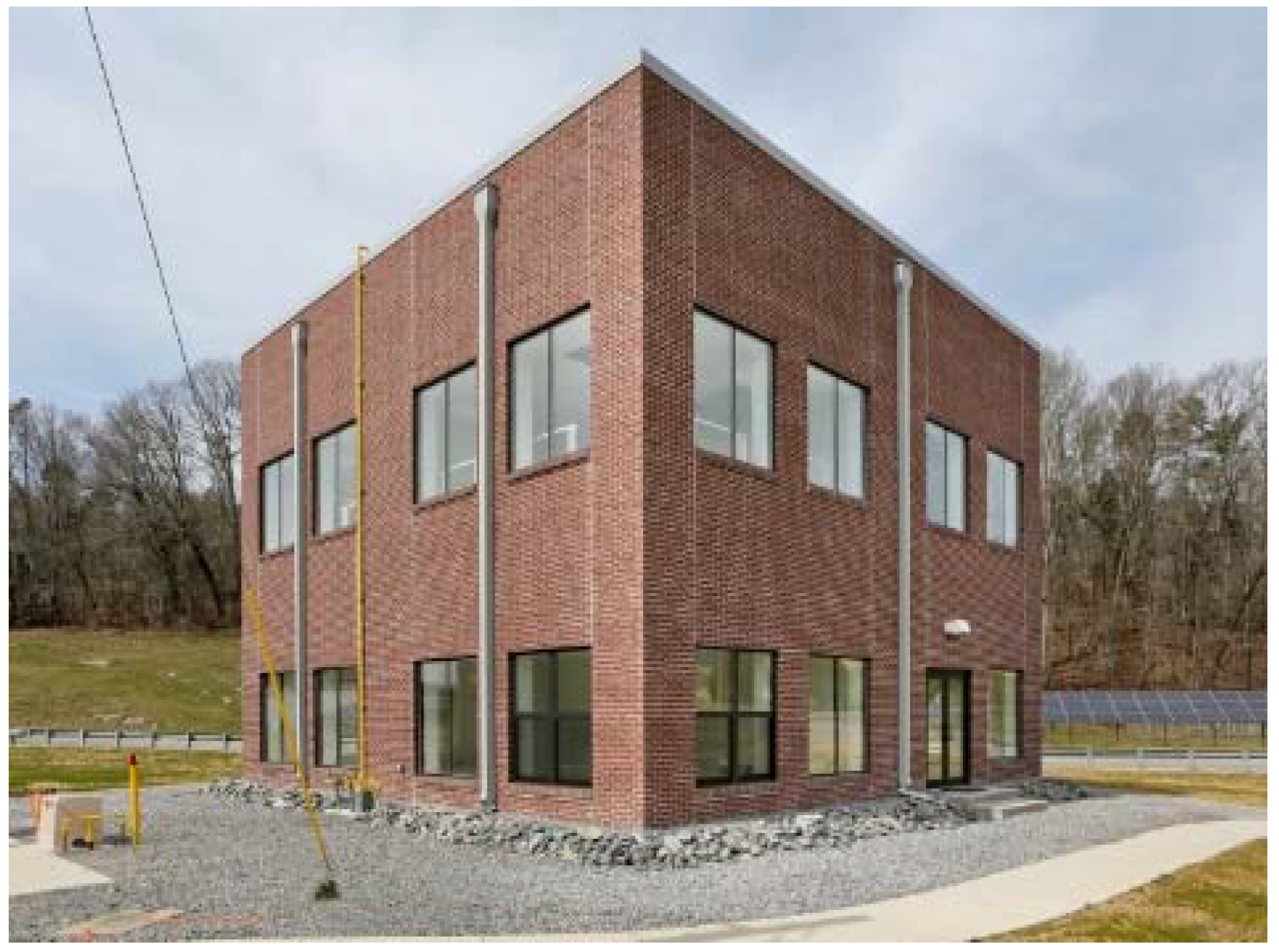
Figure 7.
System schematic and monitoring points for VRF-OAP system.
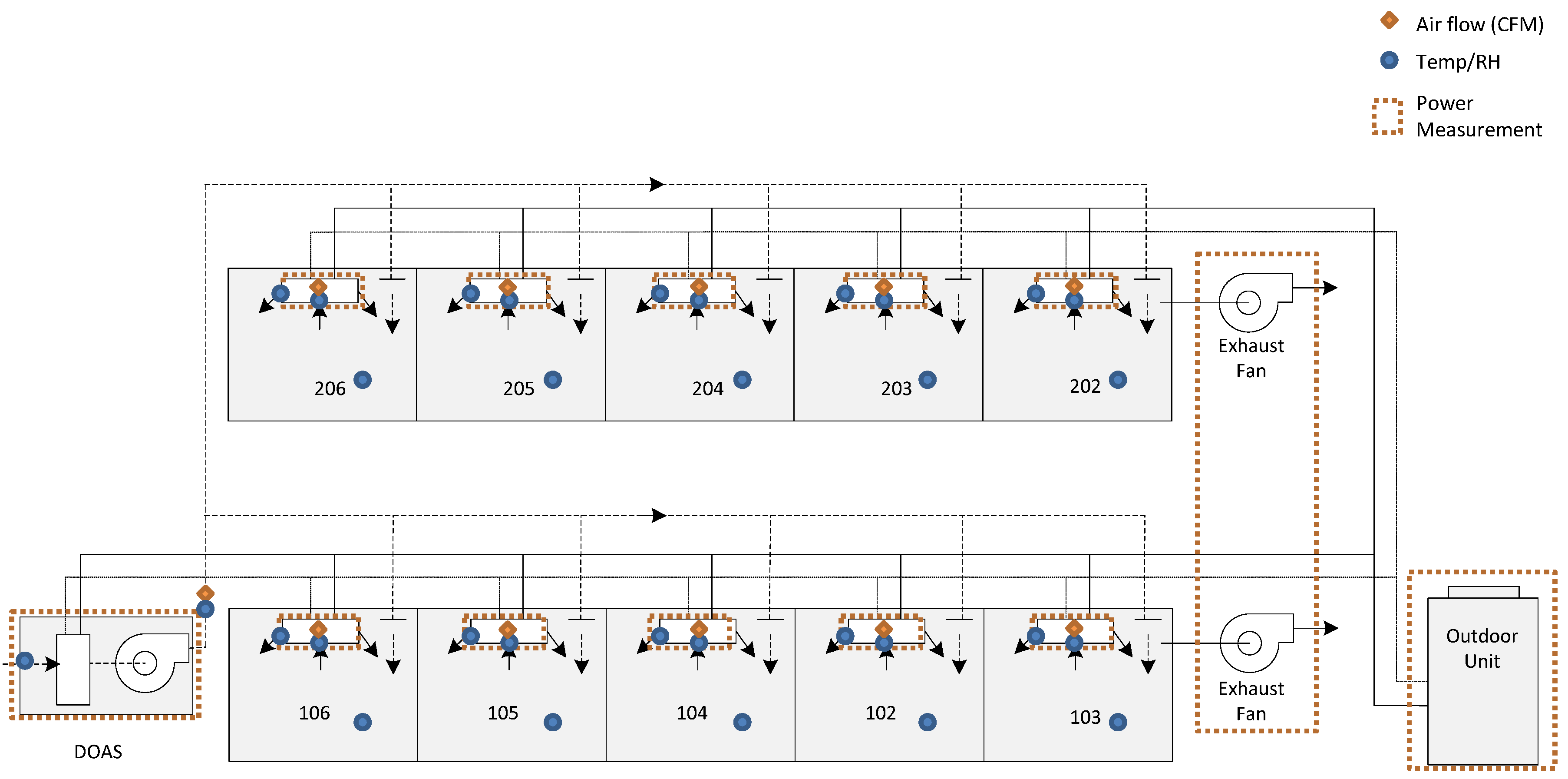
Figure 8.
Schematic of operation to emulate.

Figure 9.
Changes in supply air temperature in the OAP according to outdoor air temperature.

Figure 10.
Comparison of changes in energy consumption according to outdoor air temperature (a) 100% load; (b) 75% load; and (c) 50% load.
Figure 10.
Comparison of changes in energy consumption according to outdoor air temperature (a) 100% load; (b) 75% load; and (c) 50% load.

Figure 11.
Comparison of indoor temperature and relative humidity; (a) Conventional control (Indoor Temperature, Indoor Relative Humidity); (b) Algorithm (Indoor Temperature, Indoor Relative Humidity).
Figure 11.
Comparison of indoor temperature and relative humidity; (a) Conventional control (Indoor Temperature, Indoor Relative Humidity); (b) Algorithm (Indoor Temperature, Indoor Relative Humidity).

Table 1.
The specification of Multicalorimeter.
| Item | Outdoor Chamber | Indoor Chamber 1 | Indoor Chamber 2 |
|---|---|---|---|
| Cooling capacity | 14.5 kW–145.3 kW | 5.8 kW–58.1 kW | 5.8 kW–58.1 kW |
| Temperature range | −30–60 °C | 0–50 °C | 0–50 °C |
| Relative humidity range | 5–90% | 10–90% | 10–90% |
| Accuracy | ±2% | ±2% | ±2% |
| Repeatability | ±2% | ±2% | ±2% |
| Air flow rate | 21,000 m3/h | 8400 m3/h | 8400 m3/h |
Table 2.
Specification of VRF-OAP system.
| Unit | Specification |
|---|---|
| Outdoor Unit | Cooling capacity 81.2 kW, Integrated cooling power input 8.79 kW, Compressor: SSC Scroll X 3 Units, Fan: Propeller type X 3 Units, Refrigerant: 410 A/14.90 kg Charge, Operation temperature rage: Cooling −5–48 °C |
| Indoor Units | Cooling capacity 7.2 kW, Power input 130 W, Air flow rate 1020 m3/h |
| Outside Air Processing unit (OAP) | Cooling capacity 22.4 kW, Power input 300 W, Air flow rate 1680 m3/h, Operation temperature range: Outdoor temperature −5–52 °C, indoor supply temperature 13–25 °C (default 18 °C) |
Table 3.
Test cases.
| Case | Outdoor air Temperature (DB/WB) | Indoor Air Temperature (DB/WB) | Supply Air Temperature (DB) |
|---|---|---|---|
| Case 1 | 35 °C/24 °C | 27 °C/19 °C | 16 °C |
| Case 2 | 18 °C | ||
| Case 3 | 20 °C | ||
| Case 4 | 24 °C | ||
| Case 5 | 32 °C/23 °C | 27 °C/19 °C | 16 °C |
| Case 6 | 18 °C | ||
| Case 7 | 20 °C | ||
| Case 8 | 24 °C | ||
| Case 9 | 30 °C/22 °C | 27 °C/19 °C | 16 °C |
| Case 10 | 18 °C | ||
| Case 11 | 22 °C |
Table 4.
Changes in cooling capacity according to a supply air temperature.
| Case | Outdoor Temperature (DB/WB) (°C) | OAP Supply Set Temperature (°C) | Cooling Capacity (kW) | Rate of Change (%) | |||
|---|---|---|---|---|---|---|---|
| OAP | Code Tester 1 | Code Tester 2 | SUM | ||||
| Case 1 | 35 °C/24 °C | 16 | 17.2 | 28.1 | 30.5 | 75.8 | −0.3 |
| Case 2 | 18 | 17.4 | 28.3 | 30.3 | 76.0 | - | |
| Case 3 | 20 | 14.7 | 29.4 | 31.3 | 75.4 | −0.8 | |
| Case 4 | 24 | 11.5 | 30.7 | 32.6 | 74.8 | −1.6 | |
| Case 5 | 32 °C/23 °C | 16 | 15.5 | 29.5 | 28.5 | 73.5 | −0.4 |
| Case 6 | 18 | 12.9 | 32.9 | 28.0 | 73.8 | - | |
| Case 7 | 20 | 14.4 | 34.9 | 29.7 | 79.0 | 7.0 | |
| Case 8 | 24 | 12.0 | 35.1 | 31.1 | 78.1 | 5.8 | |
| Case 9 | 30 °C/22 °C | 16 | 12.5 | 27.2 | 28.7 | 68.4 | −2.2 |
| Case 10 | 18 | 12.4 | 28.8 | 28.8 | 69.9 | - | |
| Case 11 | 22 | 8.7 | 29.7 | 29.4 | 67.7 | −3.1 | |
Table 5.
Target building and system characteristics.
| Location | Oak Ridge, Tennessee, USA |
|---|---|
| Building size | Two-story, 40 × 40 ft. (12.2 m × 12.2 m), 14 ft. (4.3 m) floor-to-floor height |
| Exterior walls | Concrete masonry units with face brick, RUS-11 (RSI-1.9) fiberglass insulation |
| Floor | Slab-on-grade |
| Roof | Metal deck with RUS-18 (RSI-3.17) polyisocyanurate insulation |
| Windows | Double-pane clear glazing, 28% window-to-wall ratio |
| Baseloads | 0.85 W/ft2 (9.18 W/m2) lighting power density, 1.3 W/ft2 (14.04 W/m2) equipment power density |
| VRF-OAP system | 12-ton (42 kW) VRF system with a OAP |
Table 6.
Operation schedule.
| Conventional Control | Algorithm | ||
|---|---|---|---|
| Date | Load | Date | Load |
| 11 July | 50% | 14 September | 50% |
| 12 July | 15 September | ||
| 13 July | 16 September | 75% | |
| 14 July | 75% | 17 September | |
| 15 July | 18 September | ||
| 16 July | 19 September | 100% | |
| 17 July | 100% | 20 September | |
| 18 July | 21 September | 50% | |
Table 7.
Prediction results of energy consumption by outdoor air temperature through regression analysis.
Table 7.
Prediction results of energy consumption by outdoor air temperature through regression analysis.
| Outdoor Temperature (°C) | 100% Load | 75% Load | ||||
|---|---|---|---|---|---|---|
| Conventional (kWh) | Algorithm (kWh) | Saving Rates (%) | Conventional (kWh) | Algorithm (kWh) | Saving Rates (%) | |
| 20 | - | - | - | 3669.7 | 2937.2 | 20.0 |
| 21 | - | - | - | 3827.0 | 3143.8 | 17.9 |
| 22 | - | - | - | 3984.3 | 3350.4 | 15.9 |
| 23 | - | - | - | 4141.6 | 3557.0 | 14.1 |
| 24 | - | - | - | 4298.9 | 3763.6 | 12.5 |
| 25 | 6844.6 | 5690.9 | 16.9 | 4456.2 | 3970.2 | 10.9 |
| 26 | 7215.3 | 6023.3 | 16.5 | 4613.5 | 4176.8 | 9.5 |
| 27 | 7586.0 | 6355.7 | 16.2 | 4770.8 | 4383.4 | 8.1 |
| 28 | 7956.7 | 6688.1 | 15.9 | 4928.1 | 4590.0 | 6.9 |
| 29 | 8327.4 | 7020.4 | 15.7 | 5085.4 | 4796.6 | 5.7 |
| 30 | 8698.1 | 7352.8 | 15.5 | 5242.7 | 5003.2 | 4.6 |
© 2017 by the authors. Licensee MDPI, Basel, Switzerland. This article is an open access article distributed under the terms and conditions of the Creative Commons Attribution (CC BY) license (http://creativecommons.org/licenses/by/4.0/).
Share and Cite
MDPI and ACS Style
Lee, J.H.; Yoon, H.J.; Im, P.; Song, Y.-h. Verification of Energy Reduction Effect through Control Optimization of Supply Air Temperature in VRF-OAP System. Energies 2018, 11, 49. https://doi.org/10.3390/en11010049
AMA Style
Lee JH, Yoon HJ, Im P, Song Y-h. Verification of Energy Reduction Effect through Control Optimization of Supply Air Temperature in VRF-OAP System. Energies. 2018; 11(1):49. https://doi.org/10.3390/en11010049
Chicago/Turabian StyleLee, Je Hyeon, Hyun Jin Yoon, Piljae Im, and Young-hak Song. 2018. "Verification of Energy Reduction Effect through Control Optimization of Supply Air Temperature in VRF-OAP System" Energies 11, no. 1: 49. https://doi.org/10.3390/en11010049
Note that from the first issue of 2016, this journal uses article numbers instead of page numbers. See further details here.