Coordinated Control of Wind Turbine and Energy Storage System for Reducing Wind Power Fluctuation


1
Department of Electrical Engineering, Hanyang University, Seoul 133-791, Korea
2
National Renewable Energy Laboratory, Golden, CO 80401, USA
*
Author to whom correspondence should be addressed.
Energies 2018, 11(1), 52; https://doi.org/10.3390/en11010052
Submission received: 29 October 2017
/
Revised: 7 December 2017
/
Accepted: 20 December 2017
/
Published: 27 December 2017
(This article belongs to the Special Issue Distributed and Renewable Power Generation)
Abstract
:This paper proposes a method for the coordinated control of a wind turbine and an energy storage system (ESS). Because wind power (WP) is highly dependent on wind speed, which is variable, severe stability problems can be caused in power systems, especially when the WP has a high penetration level. To solve this problem, many power generation corporations or grid operators have begun using ESSs. An ESS has very quick response and good performance for reducing the impact of WP fluctuation; however, its installation cost is high. Therefore, it is important to design the control algorithm by considering both the ESS capacity and WP fluctuation. Thus, we propose a control algorithm to mitigate the WP fluctuation by using the coordinated control between the wind turbine and the ESS by considering the ESS capacity and the WP fluctuation. Using de-loaded control, according to the WP fluctuation and ESS capacity, we can expand the ESS lifespan and improve grid reliability by avoiding the extreme value of state of charge (SoC) (i.e., 0 or 1 pu). The effectiveness of the proposed method was validated via MATLAB/Simulink by considering a small power system that includes both a wind turbine generator and conventional generators that react to system frequency deviation. We found that the proposed method has better performance in SoC management, thereby improving the frequency regulation by mitigating the impact of the WP fluctuation on the small power system.
1. Introduction
Recently, wind power (WP) is incorporated in power system, and its proportion among the total power production continues to grow. Initially, the only issue considered during power generation from WP was producing the maximum amount of power from the available wind energy [1,2]. However as the proportion of the WP in a power system increased, the situation changed. As the value of the WP penetration increases, power systems have lower inertia and the power fluctuation from a wind turbine (WT) can reduce the power quality, sometimes leading to severe stability problems. Since WP is a stochastic process [3] highly dependent on turbulent fluctuations in wind speed [4,5], many studies have been carried out to integrate WP successfully without causing stability problems. To improve the stability when WP is integrated into a power system with high penetration, different methods for grid frequency regulation have been studied. And for wind power plant active power control, wake effect should be included for better performance [6].
Energy storage system (ESS) can be used to mitigate the renewable power fluctuation, shave the load peak, and level the load, as discussed in [7,8,9]. Some authors [10] also studied single or hybrid ESSs and reported that the performance was improved when using a hybrid ESS compared to a single ESS, even when compared to a previous study that investigated a single type ESS control [11]. And further control methods were introduced. For example, self-adaptive wavelet packet decomposition technique and a two-level power reference signal distribution method were used for hybrid ESS to mitigate wind power fluctuation [12]. Novel coordinated control strategy using model predictive control for power scheduling with different energy storage system (i.e., power type and energy type) [13]. Moreover, Heuristic optimization for power scheduling using particle swarm optimization method was also introduced for real-time implementation [14] and some authors introduced power fluctuation index and using this index for ESS control [15]. Distributed model predictive control was proposed to control a wind farm and an ESS efficiently [16] using short-term ESS.
Recently, some studies also have been being conducted to control an ESS considering state of Charge (SoC) of the ESS for economic operation [17,18]. In [17], authors proposed the SoC feedback control method for a WP and an ESS activating pitch control during a specific SoC region. The pitch control can be used for the SoC management but this is not appropriate for responding sudden deviation due to wind fluctuation which is a common occurrence throughout a day. The other method [18] also consider the SoC management and introduced a method that divides the different control region for the ESS. In this method, However, ESS takes all the responsibility for mitigating WP fluctuation, without any action from a WT, which can result in the capacity-related problems of the ESS and reduce its lifespan. Another method that uses a dual-layer control scheme was introduced for reducing the WP fluctuation and managing the SoC of the ESS [19]. This method also fully depends on the ESS behavior for mitigating wind power fluctuation. Therefore, previous methods mainly depends on an ESS control to mitigate WP fluctuation that requires more capacity of an ESS and reduces life span of an ESS.
In this paper, we propose a coordinated control of a WT and an ESS, which can help reduce WP fluctuation when wind speed variation suddenly increases. By changing operation of the WT as de-loaded manner according to the wind speed variation and ESS capacity size, grid reliability can be improved. Moreover, by reducing a peak-to-peak value of a SoC, an ESS can have a longer lifespan. For proper de-loaded operation considering wind variance and ESS energy capacity, we introduce a parameter and we investigate case studies with different ESS energy capacity. A small power system, which includes conventional generators, is investigated to illustrate the effectiveness of the proposed method. The results show that the proposed method is beneficial for not only reducing the WP fluctuation, but also managing the ESS SoC during the period that there is significant WP fluctuation. Using the proposed method, the reliability of the power system can be improved and the ESS can be used more effectively by changing the power production level to a slightly lower point for the de-loaded operation. There are two options (i.e., higher and lower rotor speed operation) for the de-loaded operation of a WP. Some authors suggested that a higher rotor speed operation is more beneficial for inertial response of a WP during system frequency event [20] and proved its stability. However, in terms of mitigation of a WP fluctuation, we propose the lower rotor speed de-loaded operation and illustrated the reasons and the results obtained from the method.
2. Wind Power and ESS Models
In this section, a WP and an ESS models are briefly described. For simple analysis, and to obtain meaningful tendencies, we account for the WP model by using the mechanical power of a WT. Additionally, for simplicity, a drive train and power converter dynamics are ignored in this paper. We will investigate the dynamics in greater detail in the future. However, using this simple model, we can describe a motivation and advantages of the proposed method.
2.1. Wind Power Model
To account for a WP fluctuation, we briefly describe the WP model which includes a wind speed and a power coefficient. The mechanical power from a WT, , can be obtained from the following equation:
where is the air density of the nearby area and is the blade swept area, which can be obtained from the WT blade length. The power coefficient, , is the function of the pitch angle, , and the tip speed ratio, . The and are dimensionless parameters. We used the same formulation that was introduced in [17]. The mechanical power from the WT depends on the wind speed, and its operation condition is determined by the pitch angle and rotor speed. All the values of the parameters in Equation (1) are described in Appendix A Table A1. However, this modelling remains statistical without considering the dynamics of the turbulent fluctuations in wind: this point is crucial.
2.2. ESS Power Model
We use an ESS power model, which is described in [21]. The ESS is used to compensate for WP fluctuation from a WT by charging or discharging. To mitigate the power fluctuation, the ESS is controlled to function as a low-pass filter. In [21], the ESS power is modelled as follows:
where (W) is the WP from the WT and (W) is the filtered power after the ESS mitigates the power fluctuation. (Wh) is the energy stored in the ESS, which is an important index since the capacity of the ESS should be considered. (W) is the power from the ESS, which can be defined as a high-frequency power component of the WP fluctuation, described as follows:
The usually has the form of a high-pass filter. In [10], it was proposed that the k parameter, which is dimensionless, should be introduced to manage the SoC of the ESS. k is usually 1 except in areas that are close to the extreme value (i.e., 0 or 1 (pu)) of the SoC. The preferred value of the SoC is (pu), which allows the ESS to have a large operation range in both cases (i.e., charging and discharging).
2.3. Power System Model
We consider a small power system model with the same parameters used in [17] in order to evaluate the impact of the WP fluctuation, as illustrated in Figure 1. In this system, a conventional steam turbine and hydraulic generators are included (i.e., Gen(1) Gen(2), Gen(3), respectively as described in the figure), and an automatic generation control (AGC) loop is considered. In conventional power systems, governors react to the frequency deviation as a primary frequency response and the AGC regulates the frequency to recover the nominal system frequency as a secondary frequency response. The detailed parameters of the governors and the AGC are included in the appendix.
3. Proposed Control Strategy
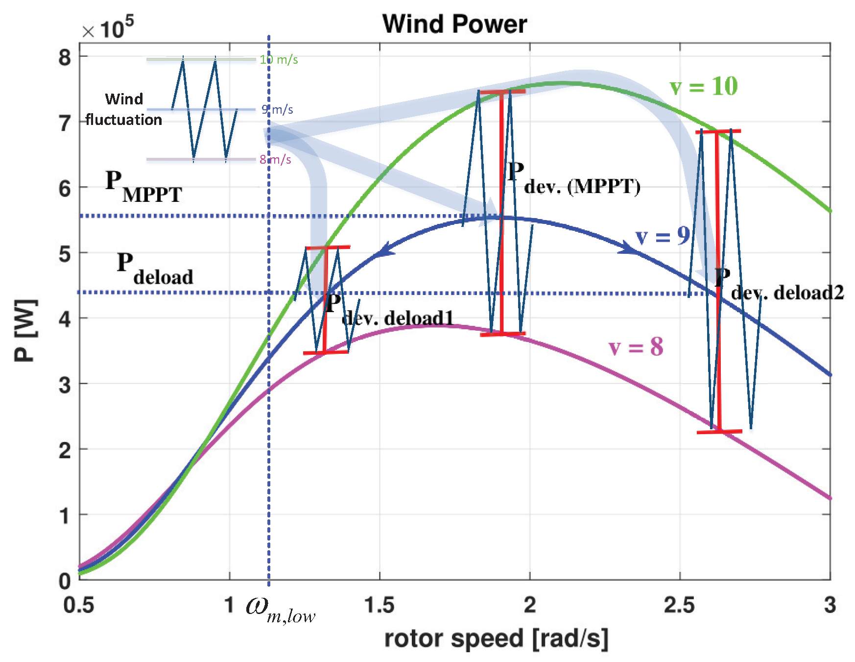
Since WP is highly dependent on wind conditions and the capacity of the ESS cannot be expanded without limitations, it is more efficient to use coordinated control of the WP and ESS. Some authors proposed ESS SoC feedback control by using pitch control to regulate the SoC and maintain a value near [10]. However, the pitch control action has a slow response and is more effective under higher wind speeds. Therefore, we investigated a method that coordinates the ESS power and WP to mitigate WP fluctuation quickly; this is done by controlling the rotor speed to manipulate the value. Figure 2 describes the WP curves at different wind speeds, and the WP increases as the wind speeds increase. As already introduced in a previous work [21], the WT can control the active power for grid support. Variable speed WT can change its operation rather than MPPT (maximum power point tracking) operation to prepare for grid event [23] (i.e., When there is frequency deviation in a grid, variable speed WT change its generation level to regulate the frequency of power system). This active power control can be accomplished when the WT operates in the de-loaded region which is not the MPPT point of WP production. Even thought there is some cost for producing the reduced power instead of the maximum available power from the WT, the WP can be flexibly adjusted according to the grid support requirement. Additionally, by highlighting the advantage of the lower-speed region for de-loaded operation, we introduce a novel strategy that uses the WT and ESS hybrid generation to mitigate the WP fluctuation. In Figure 2, the red line denotes the power fluctuation according to the wind speed variation. The lower rotor speed region results in less power fluctuation compared to the other operation regions (i.e., the MPPT and higher rotor speed regions). Therefore, it may be more helpful to operate in the lower rotor speed region when high wind variation occurs. However, for the stable operation, the de-loaded power reference should not be less than . Thus, in order to mitigate the WP fluctuation, the proposed method changes the operation point of the WT to the lower rotor speed region when there is high wind variability. Using this control scheme, the WT can reduce the burden of the ESS by mitigating the WP fluctuation. Consequently, this enables the ESS to manage the SoC successfully, avoiding extreme values, thereby expanding the ESS life span. Moreover, the impact of the WP fluctuation on the grid frequency can be reduced because the ESS cannot be dedicated to regulating the power fluctuation because of its limited energy capacity.
To consider the wind power fluctuation into both ESS and WT control, we investigated the wind power fluctuation induced from wind speed variability. From the WT power model, we can obtain the following equations.
where, is average wind speed and is wind speed variation.
For small , can be approximated same as
In addition, can be also approximated by
where, is average wind power relating with average wind speed and is wind power fluctuation resulting from wind speed variation component. Thus, we can find out that the WP fluctuation induced from wind speed variation is proportional to the second term in the above equation. Therefore the wind power fluctuation is related with averaged wind speed, and we use this relation when determining the deloading operation. We defined a parameter, to determine the deloading operating point using above WP fluctuation equation and ESS capacity.
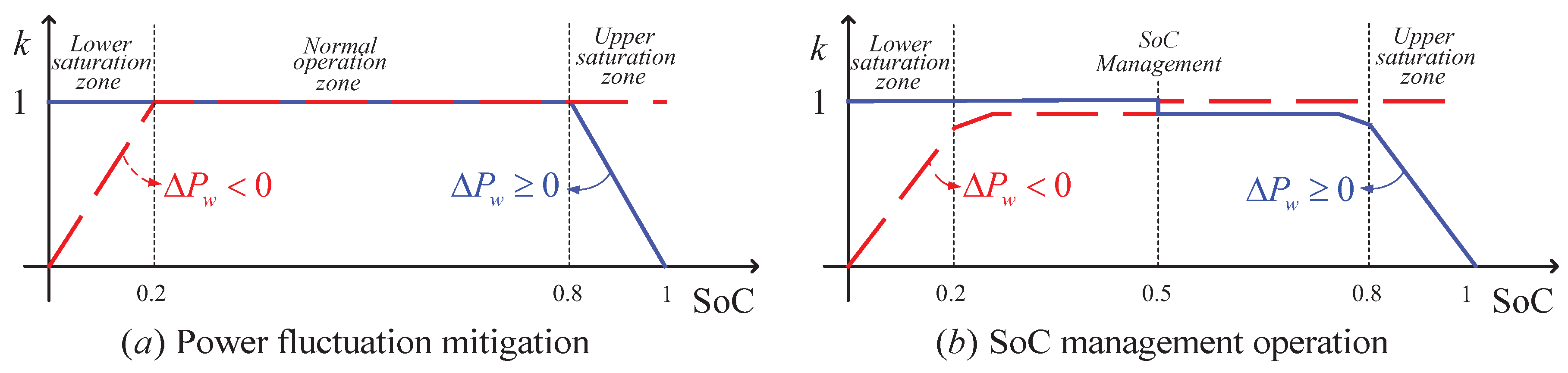
where, is the size of ESS and is a constant for scaling factor. When the capacity of ESS is large enough, then the WT does not have to reduce its power by deloading operation for reducing WP fluctuation. This is due to the fact that the ESS can handle whole WP fluctuation as the capacity of ESS is large enough. And we also relates the average wind power since that value can affect level of the WP fluctuation as described in Equation (5). From these considerations of average wind speed and capacity of an ESS in the formulation of parameter , we can adapt this formulation to different size of WT or ESS using above Equation (8). Figure 3 illustrates the ESS control strategy that was previously introduced in [24]. The k parameter is included to manage the SoC of the ESS, which has a value between 0 and 1, to reduce its action when the SoC value is extreme (i.e., when fully charging or discharging). This method was already introduced in previous work and we added additional operation defining different k function curve according to SoC to enhance the SoC management during normal wind variation condition as described in Figure 4. Therefore, we designed the method that the WT reduces its power according to the wind speed variation to reduce the burden of the ESS mitigating the WP fluctuation as shown in Figure 5. According to the wind speed variation, WT reduces its power proportional to the wind speed variation, and inverse proportional to capacity of ESS by adjusting the parameter, , when it overs the variation limit, .
4. Simulation Results
To validate the performance of the proposed algorithm, MATLAB/Simulink (2015b, MathWorks, Natick, MA, USA) was used for the power system with a WT incorporating an ESS. A small power system was investigated using the governors and AGC to evaluate the impact of WP fluctuation on the power system frequency. We assume that the wind speed measurement updates every second. First, we considered the WP fluctuation with normal variation (i.e., a value of ). After that, we considered the specific cases when the WP fluctuation suddenly increased from to with different average wind speeds (i.e., 10, 13 m/s). The wind speed profile was considered, as shown in Figure 6, as a normal case. We compared the SoC variations with different control strategies (i.e., MPPT and de-loaded operation) as described in Figure 7. Both values of the SoC are within the reliable region because the WP fluctuation was not significant. Additionally, the SoC variation was slightly less for the de-loaded operation, as was expected. We investigated the system frequency deviation, and both methods had a slight deviation, as shown in Figure 8. The frequency deviated more during MPPT operation compared to de-loaded operation, but this difference was not significant. Figure 9 compares WP productions between MPPT and deloaded operation. MPPT operation produces more power from the WT. Therefore, it is more beneficial to operate as MPPT during normal condition since there is no significant frequency event while producing more power from the WT.
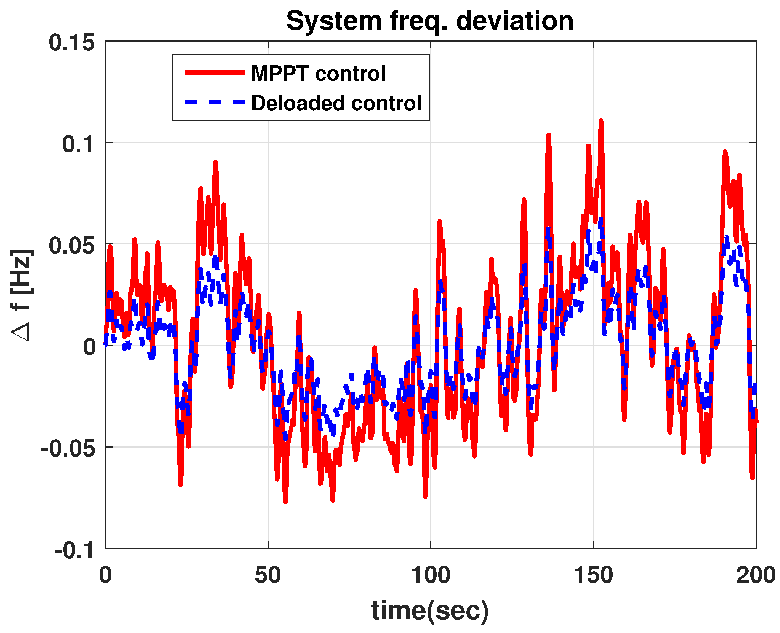
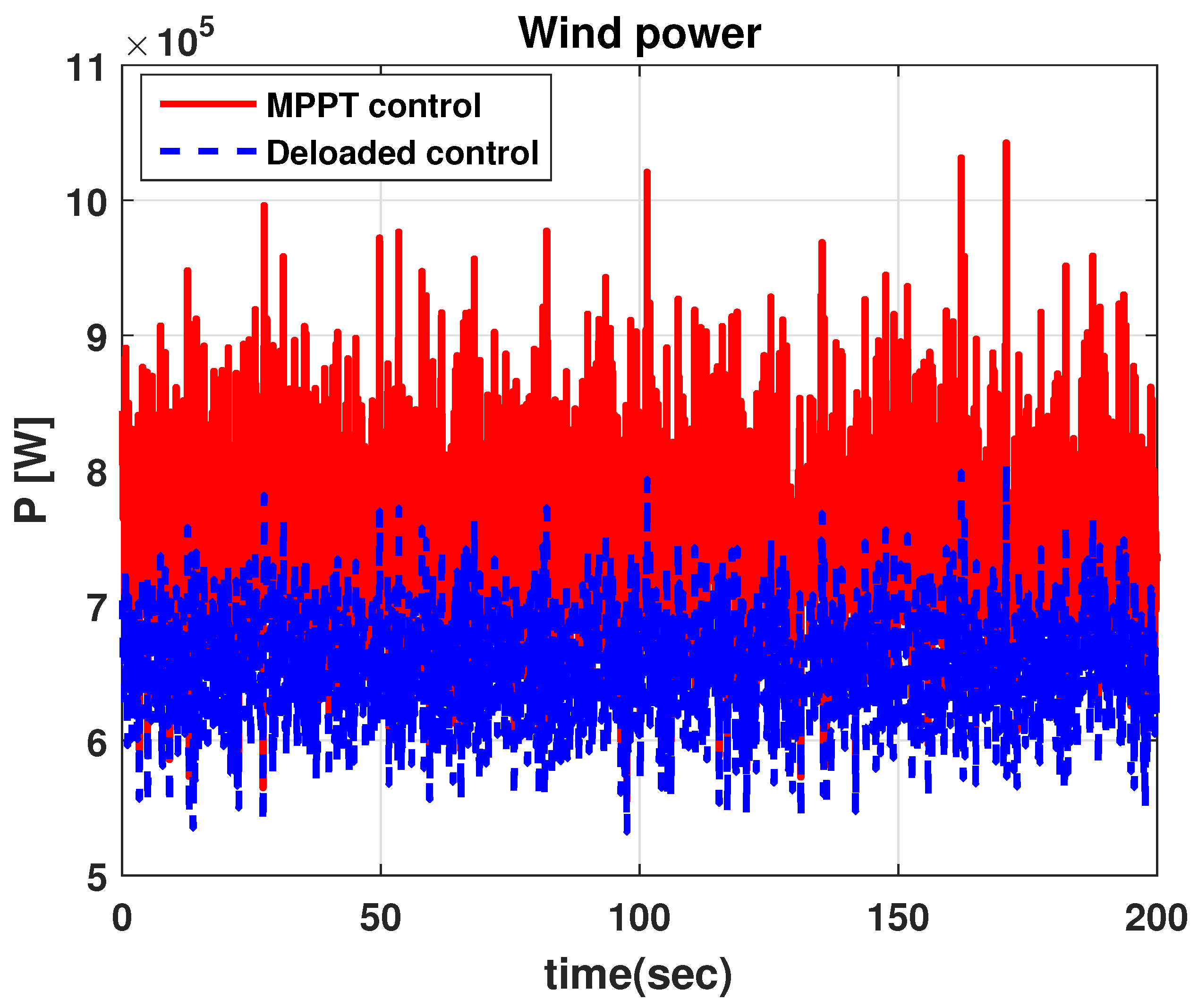
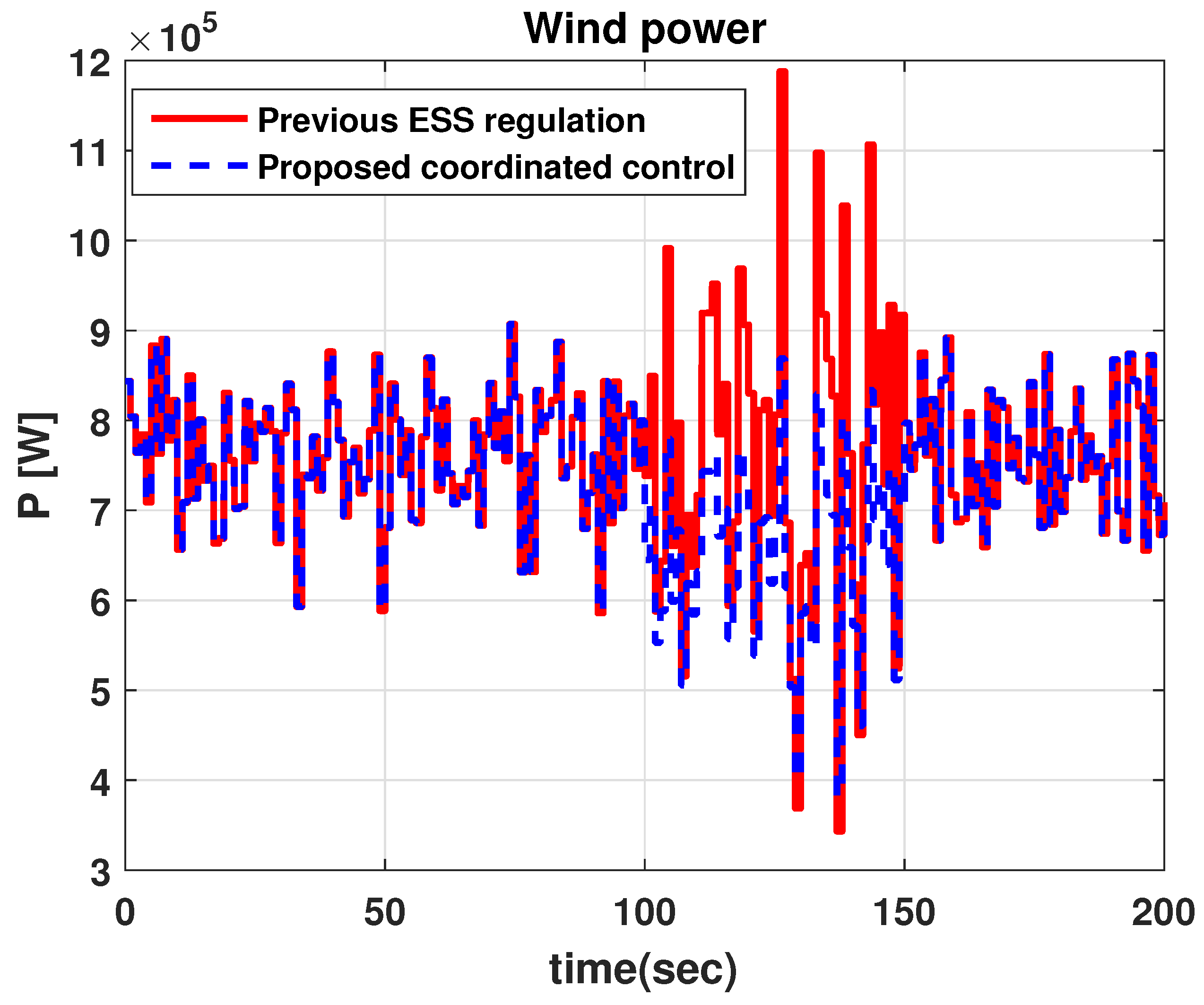
Figure 10 describes another wind speed profile that was considered in the simulation case study. We investigated variable wind speed fluctuation and some significant wind speed fluctuations over a specific period. From 100 s to 150 s, there were sudden wind speed fluctuations, and we compared the results of the proposed method and the conventional MPPT method. In this case, during this period (i.e., from 100 s to 150 s), the WT experiences de-loaded operation for the proposed method. The WP fluctuations are different during the sudden variation period (from 100 s to 150 s), as described in Figure 11, according to the wind speed variation. The WP fluctuation was reduced for the proposed method, even though the WP production had a lower mean value. When the WT produces maximum power during this sudden wind variation period, this power fluctuation has a negative effect on the ESS health, resulting in a reduced ESS lifespan. Additionally, the grid stability is decreased by the induced frequency deviation. By reducing power production, the burden of the ESS for supporting wind power fluctuation can be reduced; this can be more effective when the SoC of the ESS is closer to a critical value (i.e., 0 or 1). After around 130 s, the SoC value was much higher than in the case of the conventional MPPT method. When the value was over , the ESS reduced its charging action to manage its SoC value. Also, when the charging action of the ESS was reduced, the grid frequency increased because of its reduced charging action. The SoC of the ESS is more stable when the proposed method is used as described in Figure 12. As shown in this figure, the SoC was near in the case of the conventional method, which means that the ESS could not respond well during that period. Alternatively, the SoC can be effectively managed with less fluctuation and at a value that is even closer to when using the proposed method. We investigated the difference in the impact on the system frequency during that period, as described in Figure 13. We found that the system frequency fluctuated in the conventional case because the SoC value was close to 1, which results in a lower k parameter for managing the SoC. The ESS should be less active as a function of WP fluctuation in order to avoid reaching the capacity limit of the ESS. That is, the burden of the ESS to regulate the WP fluctuation increases during that period and requires a greater ESS capacity. Alternatively, the power fluctuation was reduced by decreasing the power production in the proposed method, thereby reducing the burden of the ESS in the proposed method. We also investigated same case study when the average wind speed is 13 (m/s). The results are illustrated from Figure 14, Figure 15, Figure 16 and Figure 17. The overall tendency was similar but, in this case, the SoC variation was over 0.9 in MPPT operation. The frequency impact is also quite severe in this case. Additional ESS capacity is needed for MPPT operation, however, the proposed method could properly respond to this WP fluctuation. Thus, the need for ESS capacity could be reduced from the proposed method and moreover, the lifespan of the ESS could be improved due to less peak to peak SoC variations.
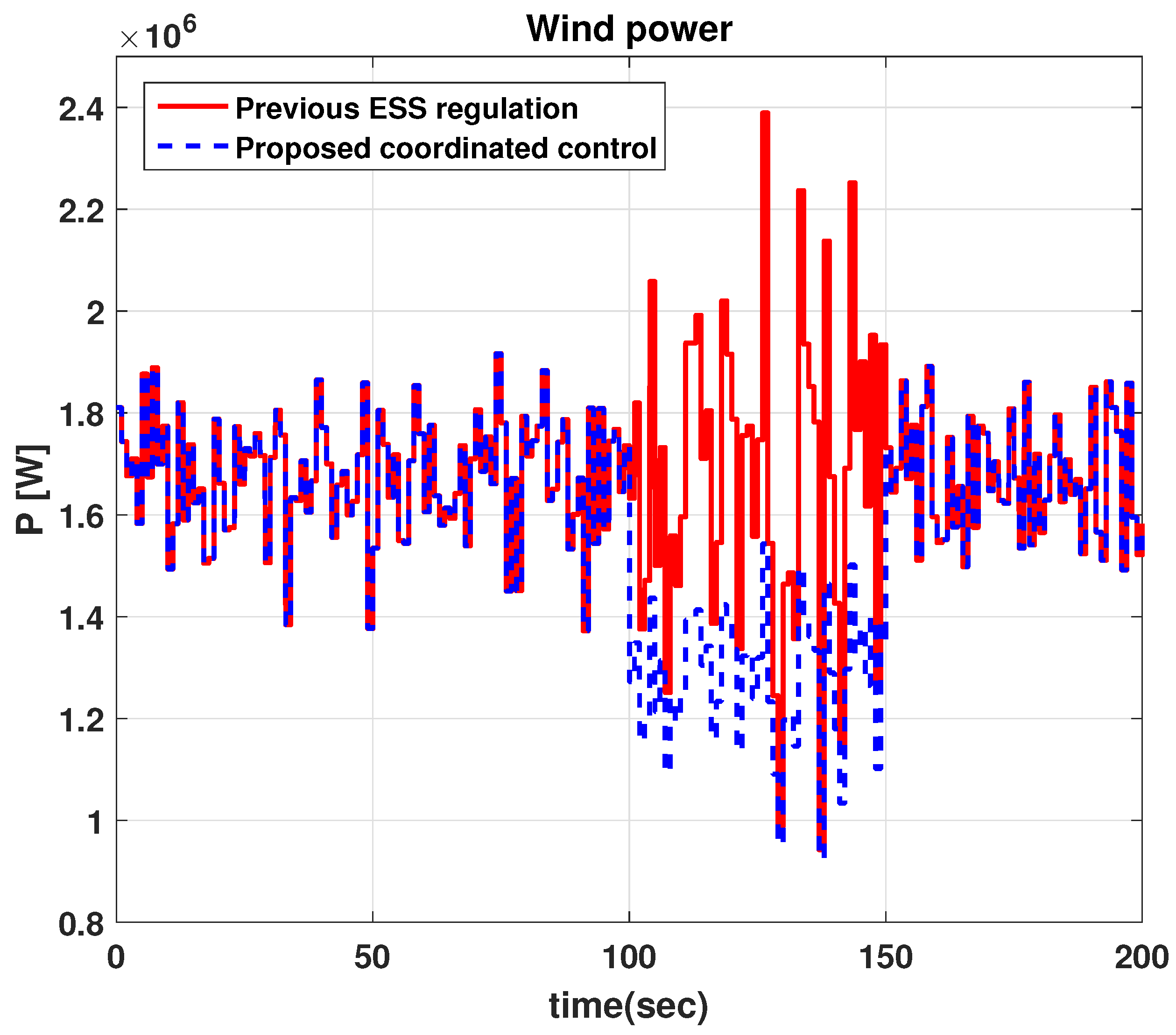
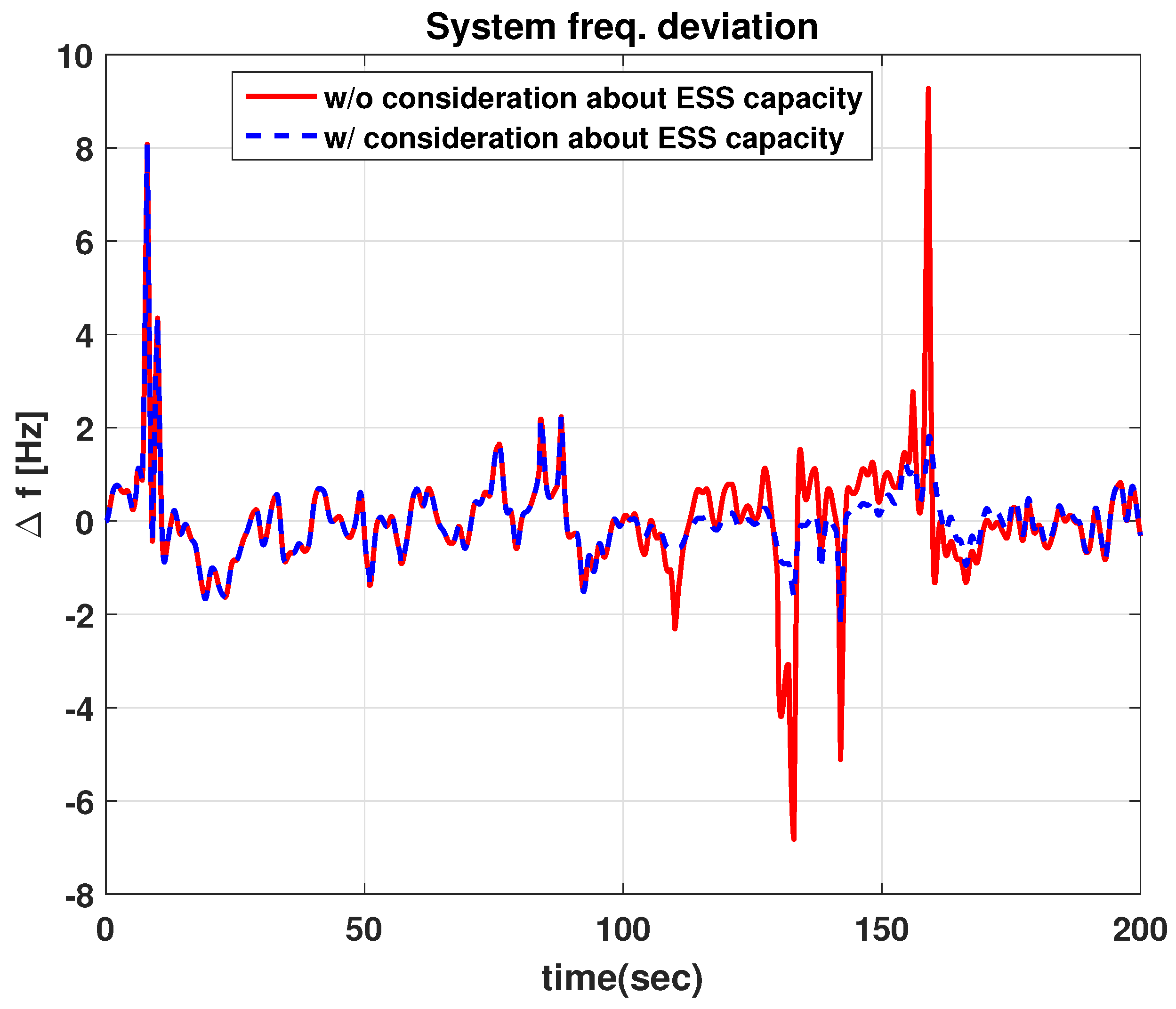
We also investigated the effect of consideration about the ESS capacity when deciding parameter. From Figure 18, Figure 19 and Figure 20, we illustrated the results when the less ESS energy capacity as 277 Wh which is half of the value of previous simulation case. In Figure 18, the production of WP is reduced when the ESS capacity is reduced and obtained less WP fluctuation, which results in less peak to peak variation in ESS SoC value in Figure 19. Moreover, the proposed method has better performance in system frequency deviation in Figure 20. Therefore, proposed method has better performance both in SoC and frequency response.
5. Conclusions
In this paper, we proposed the coordinated control of a WT and an ESS, which can help reduce WP fluctuation when the wind speed variation suddenly increases. By changing the operation of the WT to a de-loaded method according to the wind variability, the grid reliability can be improved. Moreover, the lifespan of the ESS can be increased by reducing the peak to peak value of the SoC. A small power system with conventional generators is investigated to illustrate the effectiveness of the proposed method. The results showed that the proposed method is beneficial for both reducing the wind power fluctuation and managing the ESS SoC. However, the modelling of wind power remains statistical without considering the dynamics of the turbulent fluctuations in wind: this point is crucial. Thus, we will analyze this complex aerodynamics as a future work. Furthermore, various cases with large power system should be handled considering transmission and generation units characteristics and optimization of the parameter can be investigated with different ESS sizes.
Acknowledgments
This research was supported by the Korea Electric Power Corporation (grant number: R17XA05-56). This work was performed in part at NREL (National Renewable Energy Laboratory) while the first author was visiting.
Author Contributions
Chunghun Kim designed the algorithm and developed the simulation; Eduard Muljadi provided guidance in designing the algorithm;Chung Choo Chung verified the simulation model; and all authors reviewed and approved the manuscript.
Conflicts of Interest
The authors declare no conflict of interest.
Nomenclature
| AGC | Automated Generation Control. |
| A | Blade swept area (m) |
| Scaling factor for defining de-loaded operation parameter | |
| Wind turbine power efficiency coefficient | |
| Energy capacity of an ESS (Wh) | |
| De-loaded operation parameter | |
| k | Parameter for SoC management |
| Wind power (W) | |
| Filtered wind power (low frequency component) (W) | |
| ESS charging power (W) | |
| Wind power fluctuation (W) | |
| Power variation of conventional generator, i (W) | |
| De-loaded power factor indicating reduced power proportion | |
| State of Charge (pu) | |
| Wind speed variance | |
| Average wind speed (m/s) | |
| Wind speed variance limit for deciding when de-loaded operation starts | |
| Stored energy of an ESS (Wh) | |
| air density (kg/m) | |
| Grid frequency variation (Hz) | |
| Turbine mechanical rotor speed (pu) | |
| Tip speed ratio of WT variable | |
| WT blade pitch angle (deg) |
Appendix A
The detailed parameters were used as introduced in [22].

Table A1.
System parameters used in the simulation.
| Parameter | Value | Unit |
|---|---|---|
| Sampling time | 1 | s |
| Rated power | 2 | MW |
| Rated wind speed | 13.8 | m/s |
| Average wind speed | 10 & 13 | m/s |
| Wind speed random variance | 0.1 to 0.5 | |
| Max.power coeff. | 0.4382 | |
| Optimal tip speed ratio | 6.32 | |
| Blade radius | 30 | m |
| Air density | 1.225 | kg/m |
| 0.51 | ||
| 0.2 | ||
| 555 (1 pu) | Wh |
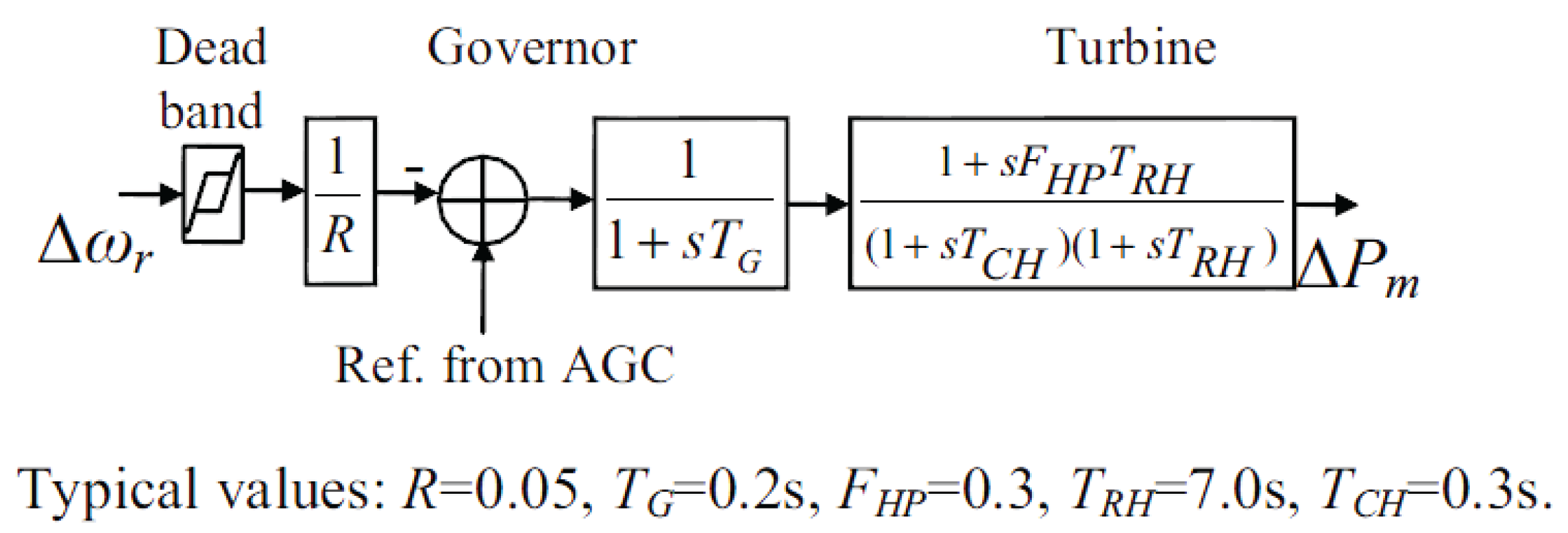
Figure A1.
Primary frequency control of a generating unit with a reheat steam turbine [22].
Figure A1.
Primary frequency control of a generating unit with a reheat steam turbine [22].

Figure A2.
Primary frequency control of a generating unit with a non-reheat steam turbine [22].
Figure A2.
Primary frequency control of a generating unit with a non-reheat steam turbine [22].
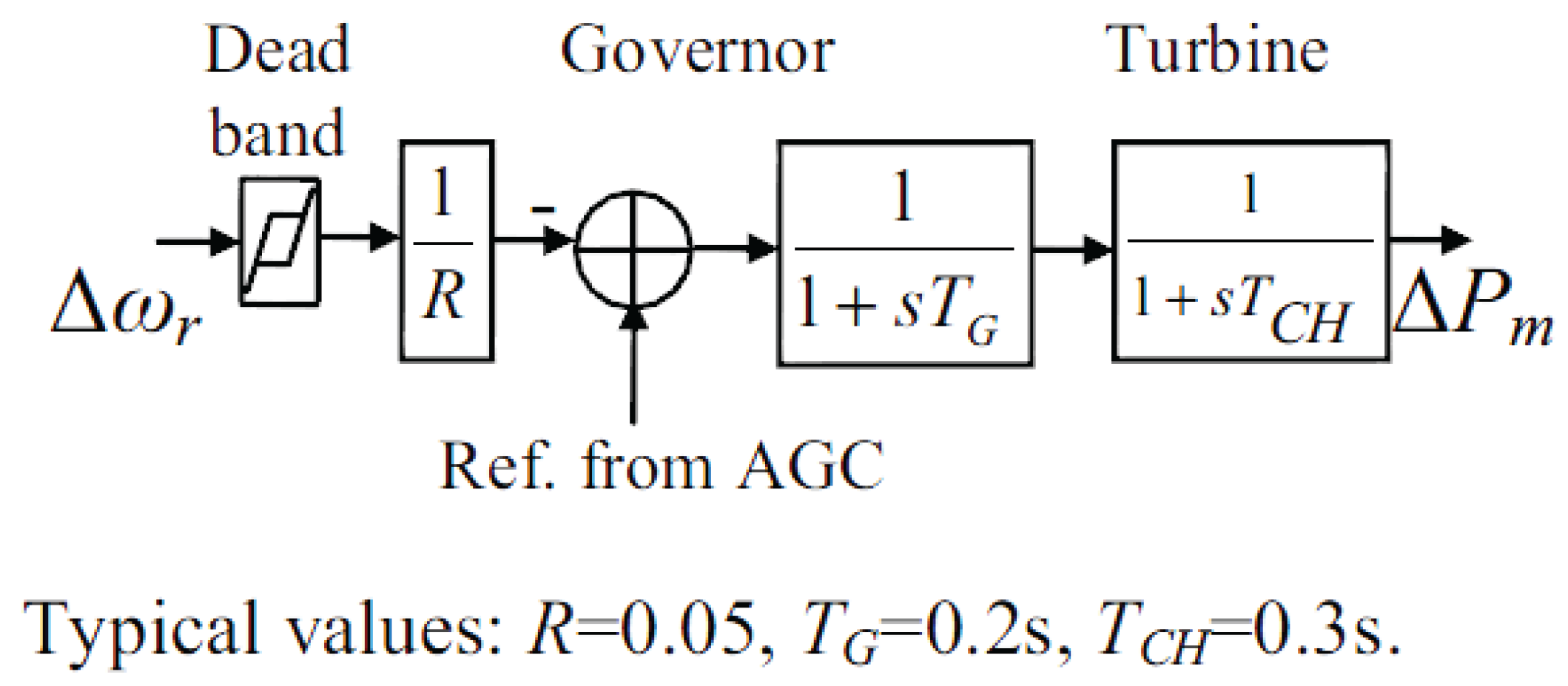
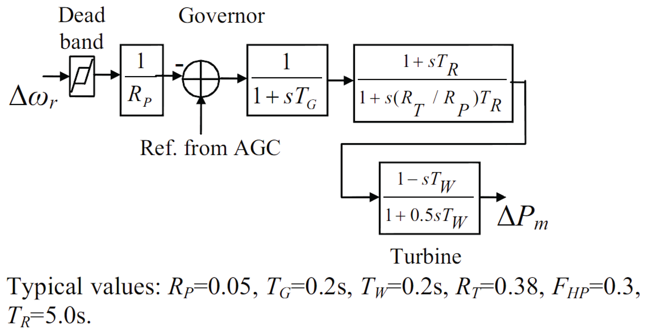
Figure A3.
Primary frequency control of a hydraulic unit [22].
Figure A3.
Primary frequency control of a hydraulic unit [22].

References
- Kim, C.; Gui, Y.; Chung, C.C. Maximum Power Point Tracking of a Wind Power Plant with Predictive Gradient Ascent Method. IEEE Trans. Sustain. Energy 2017, 8, 685–694. [Google Scholar] [CrossRef]
- Kim, C.; Gui, Y.; Chung, C.C.; Kang, Y.-C. A Model-Free Method for Wind Power Plant Control with Variable Wind. In Proceedings of the IEEE Power Energy Society General Meeting, National Harbor, MD, USA, 27–31 July 2014; pp. 1–5. [Google Scholar]
- Calif, R.; Schmitt, F.G.; Huang, Y. Multifractal Description of Wind Power Using Arbitrary Order Hilbert Spectral Analysis. Phys. A Stat. Mech. Appl. 2013, 392, 4106–4120. [Google Scholar] [CrossRef]
- Calif, R.; Schmitt, F.G. Modeling of atmospheric wind speed sequence using a lognormal continuous stochastic equation. J. Wind Eng. Ind. Aerodyn. 2012, 109, 1–8. [Google Scholar] [CrossRef]
- Calif, R.; Schmitt, F.G. Multiscaling and Joint Multiscaling Description of the Atmospheric Wind Speed and The Aggregate Power Output from a Wind Farm. J. Wind Eng. Ind. Aerodyn. 2014, 21, 379–392. [Google Scholar] [CrossRef] [Green Version]
- Kim, C.; Gui, Y.; Chung, C.C. Coordinated Wind Power Plant Control for Frequency Support under Wake Effects. In Proceedings of the IEEE Power Energy Society General Meeting, Denver, CO, USA, 26–30 July 2015; pp. 1–5. [Google Scholar]
- Vazquez, S.; Lukic, S.M.; Galvan, E.; Franquelo, L.G.; Carrasco, J.M. Energy Storage Systems for Transport and Grid Applications. IEEE Trans. Ind. Electron. 2010, 57, 3881–3895. [Google Scholar] [CrossRef]
- Wang, W.; Mao, C.; Lu, J.; Wang, D. An Energy Storage System Sizing Method for Wind Power Integration. Energies 2013, 6, 3392–3404. [Google Scholar] [CrossRef]
- Zhao, H.; Wu, Q.; Hu, S.; Xu, H.; Rasmussen, C.N. Review of Energy Storage System for Wind Power Integration Support. Appl. Energy 2015, 137, 545–553. [Google Scholar] [CrossRef]
- Li, W.; Joós, G. Comparison of energy storage system technologies and configurations in a wind farm. In Proceedings of the IEEE Power Electronics Specialists Conference, Orlando, FL, USA, 17–21 June 2007; pp. 1280–1285. [Google Scholar]
- Kook, K.S.; McKenzie, K.J.; Liu, Y.; Atcitty, S. A Study on applications of Energy Storage for the Wind Power Operation in Power Systems. In Proceedings of the IEEE Power Energy Society General Meeting, Montreal, QC, Canada, 18–22 June 2006; pp. 1–5. [Google Scholar]
- Ding, M.; Wu, J. A Novel Control Strategy of Hybrid Energy Storage System for Wind Power Smoothing. Electr. Power Compon. Syst. 2017, 45, 1265–1274. [Google Scholar] [CrossRef]
- Tang, X.; Sun, Y.; Zhou, G.; Miao, F. Coordinated Control of Multi-Type Energy Storage for Wind Power Fluctuation Suppression. Energies 2017, 10, 1212. [Google Scholar] [CrossRef]
- Yang, J.-S.; Choi, J.-Y.; An, G.-H.; Choi, Y.-J.; Kim, M.-H.; Won, D.-J. Optimal Scheduling and Real-Time State-of-Charge Management of Energy Storage System for Frequency Regulation. Energies 2016, 9, 1010. [Google Scholar] [CrossRef]
- Shi, J.; Lee, W.-J.; Liu, X. Generation Scheduling Optimization of Wind-Energy Storage System Based on Wind Power Output Fluctuation Features. IEEE Trans. Ind. Appl. 2017, 1–7. [Google Scholar] [CrossRef]
- Zhao, H.; Wu, Q.; Guo, Q.; Sun, H.; Xue, Y. Optimal Active Power Control of a Wind Farm Equipped with Energy Storage System based on Distributed Model Predictive Control. IET Gener. Transm. Distrib. 2016, 10, 669–677. [Google Scholar] [CrossRef] [Green Version]
- Dang, J.; Seuss, J.; Suneja, L.; Harley, R.G. SoC Feedback Control for Wind and ESS Hybrid Power System Frequency Regulation. IEEE J. Emerg. Sel. Top. Power Electron. 2014, 2, 79–86. [Google Scholar] [CrossRef]
- Yun, J.Y.; Yu, G.; Kook, K.S.; Rho, D.H.; Chang, B.H. SoC-based Control Strategy of Battery Storage System for Power System Frequency Regulation. Trans. Korean Inst. Electr. Eng. 2014, 63, 622–628. [Google Scholar] [CrossRef]
- Jiang, Q.; Gong, Y.; Wang, H. A Battery Energy Storage System Dual-Layer Control Strategy for Mitigating Wind Farm Fluctuations. IEEE Trans. Power Syst. 2013, 28, 3263–3273. [Google Scholar] [CrossRef]
- Buckspan, A.; Pao, L.; Aho, J.; Fleming, P. Stability Analysis of a Wind Turbine Active Power Control System. In Proceedings of the American Control Conference, Washington, DC, USA, 17–19 June 2013; pp. 1418–1423. [Google Scholar]
- Muljadi, E.; Butterfield, C.P.; Parsons, B.; Ellis, A. Effect of Variable Speed Wind Turbine Generator on Stability of a Weak Grid. IEEE Trans. Energy Convers. 2007, 22, 29–36. [Google Scholar] [CrossRef]
- Li, W.; Joós, G.; Abbey, C. Wind Power Impact on System Frequency Deviation and an ESS based Power Filtering Algorithm Solution. In Proceedings of the IEEE Power Systems Conference and Exposition, Atlanta, GA, USA, 29 October–1 November 2006; pp. 2077–2084. [Google Scholar]
- Loukarakis, E.; Margaris, I.; Moutis, P. Frequency Control Support and Participation Methods Provided by Wind Generation. In Proceedings of the IEEE Electrical Power Energy Conference, Montreal, QC, Canada, 22–23 October 2009; pp. 1–6. [Google Scholar]
- Li, W. An Embedded Energy Storage System for Attenuation of Wind Power Fluctuations. Ph.D. Thesis, McGill University, Montreal, QC, Canada, May 2010. [Google Scholar]
Figure 1.
The power system frequency control structure (modified from [22]).
Figure 1.
The power system frequency control structure (modified from [22]).
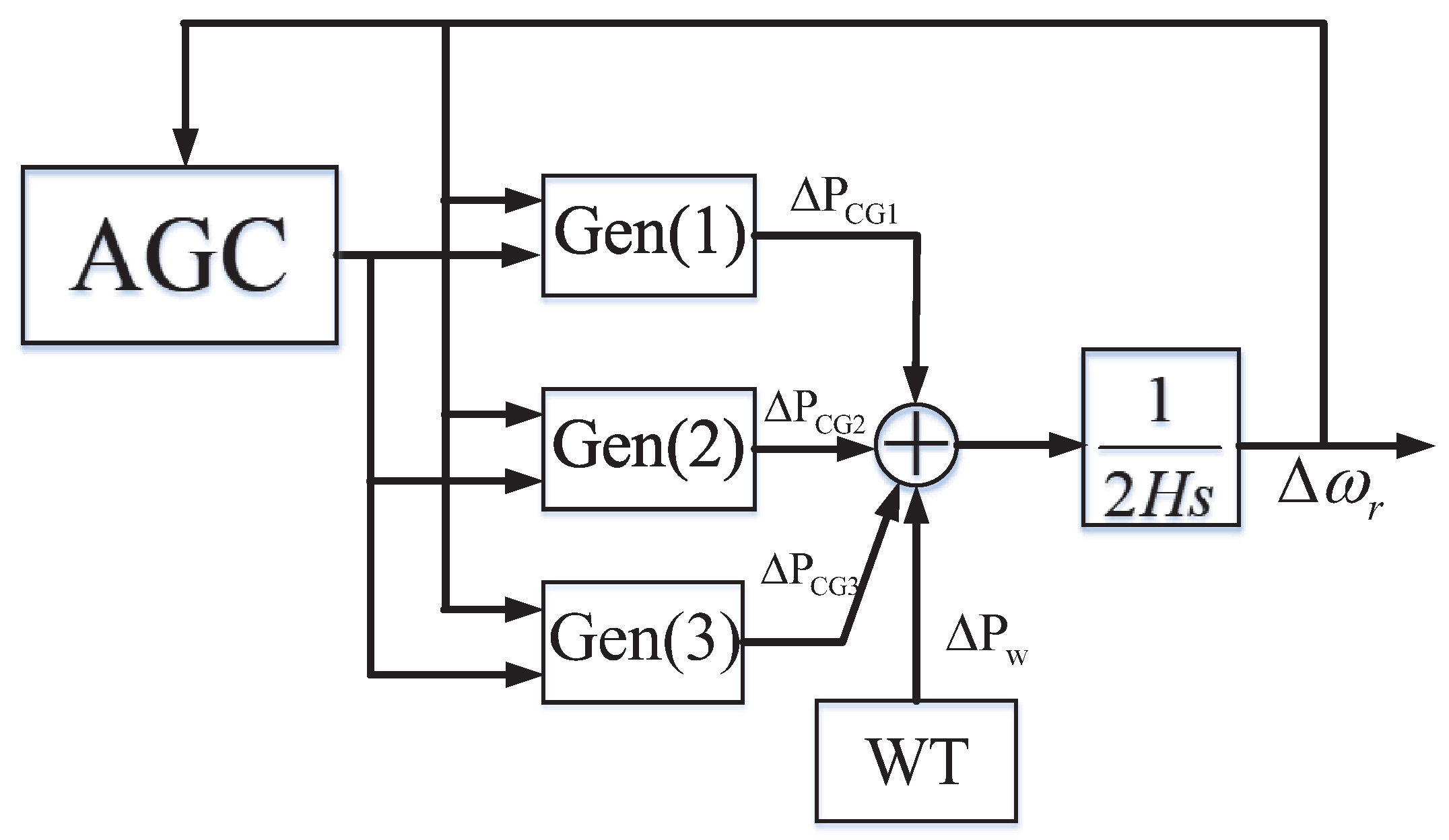
Figure 2.
Power curve with different wind speeds (8, 9, 10 m/s) for maximum power point tracking and de-loaded control. indicates the power deviation under lower rotor speed de-loaded operation and indicates the power deviation under higher rotor speed de-loaded operation. is quite small compared to and is more beneficial for mitigating wind power fluctuation.

Figure 3.
Energy storage system control and energy management scheme (modified from [24]).
Figure 3.
Energy storage system control and energy management scheme (modified from [24]).
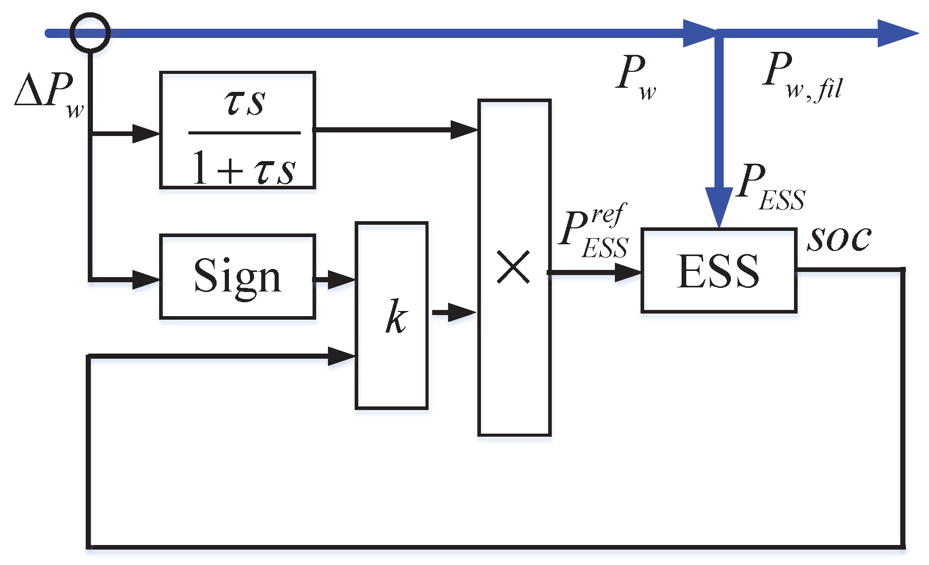
Figure 4.
Description of the value of parameter k according to the SoC (State of Charge) modified from [20]. Operation (a) is activated when abnormal wind variation () and (b) is activated when the wind variation is normal ().
Figure 4.
Description of the value of parameter k according to the SoC (State of Charge) modified from [20]. Operation (a) is activated when abnormal wind variation () and (b) is activated when the wind variation is normal ().

Figure 5.
Flow chart of the proposed control method.
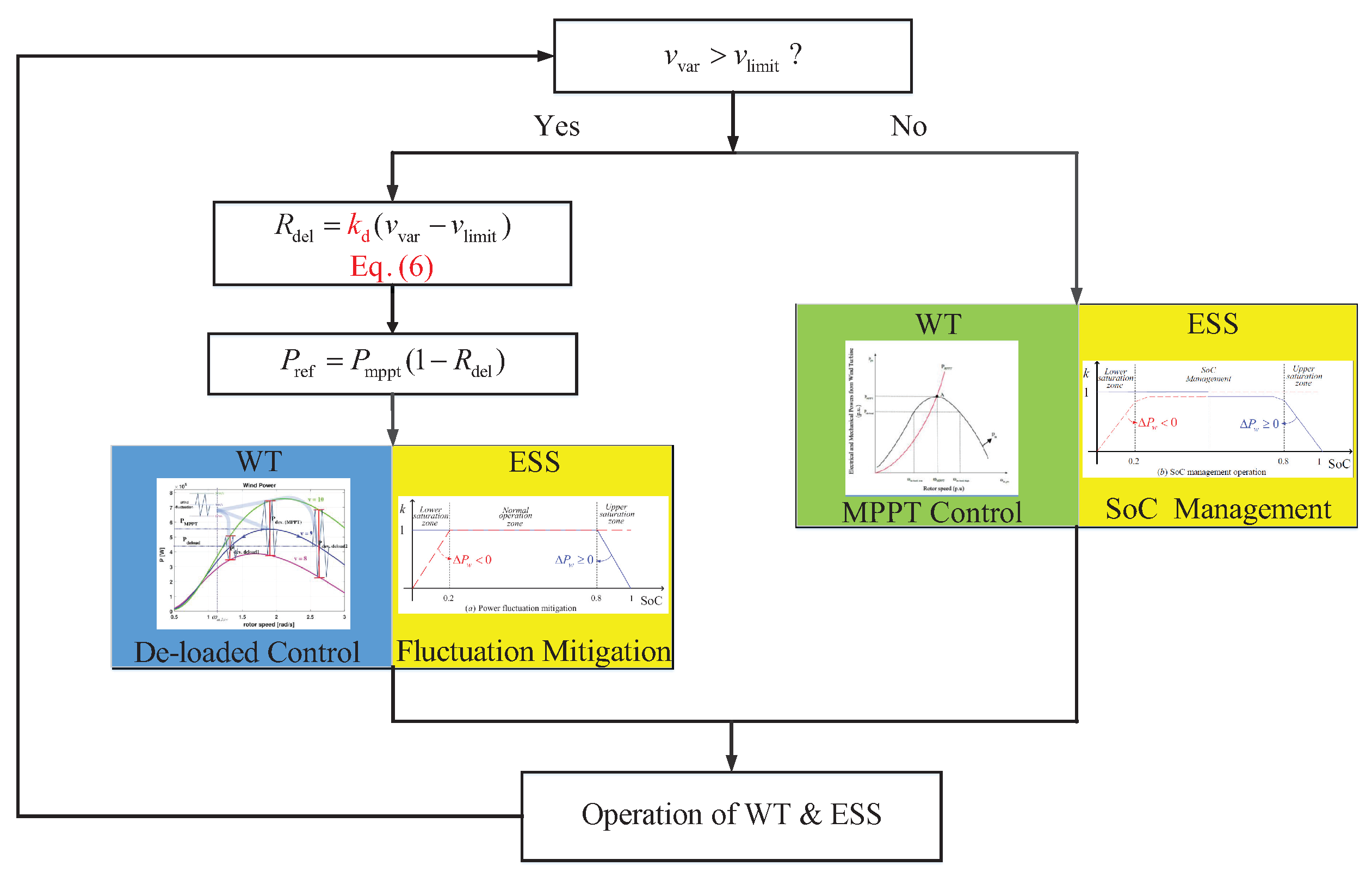
Figure 6.
Random wind speed profile.
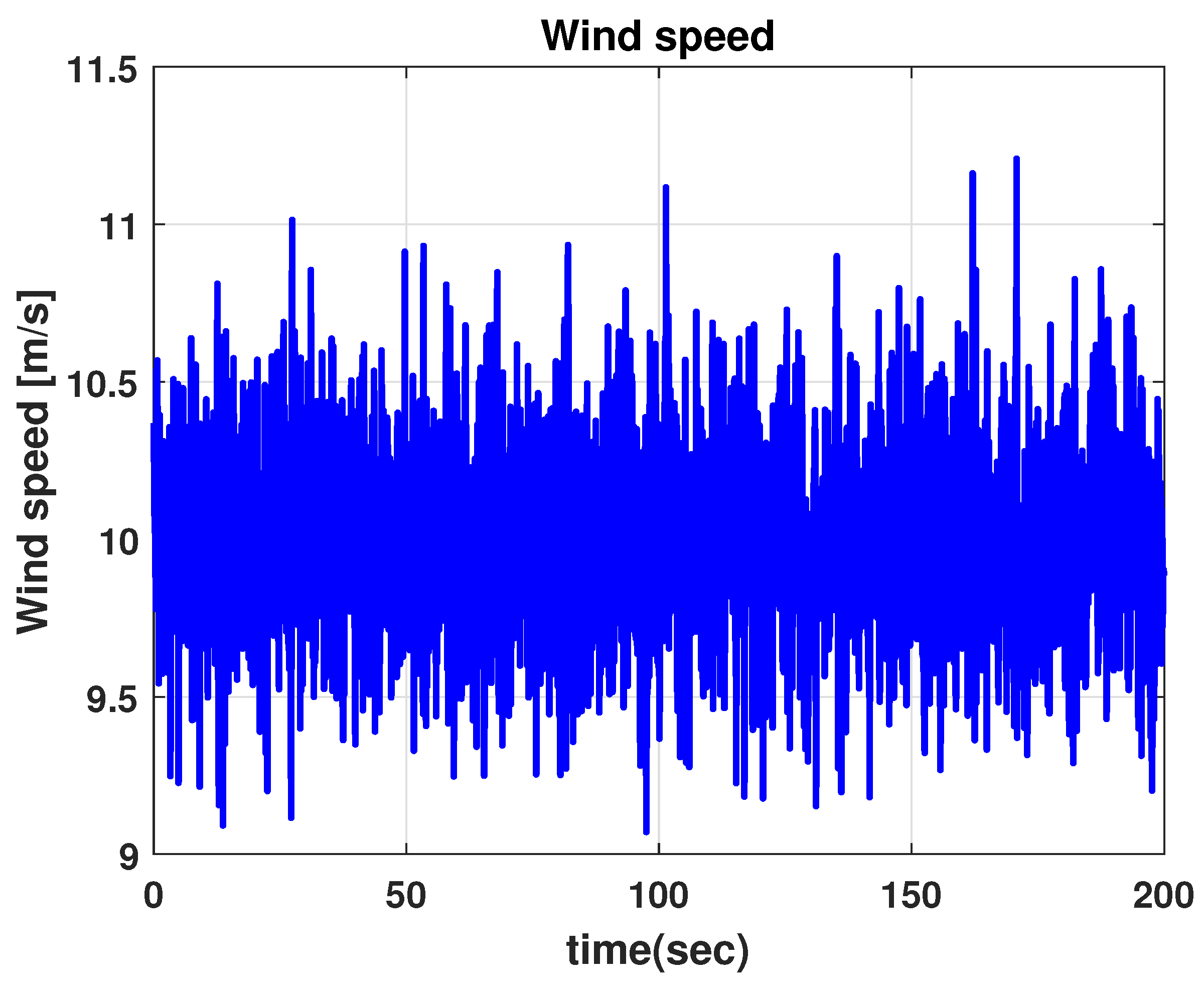
Figure 7.
Comparison of the ESS SoC for the different methods.
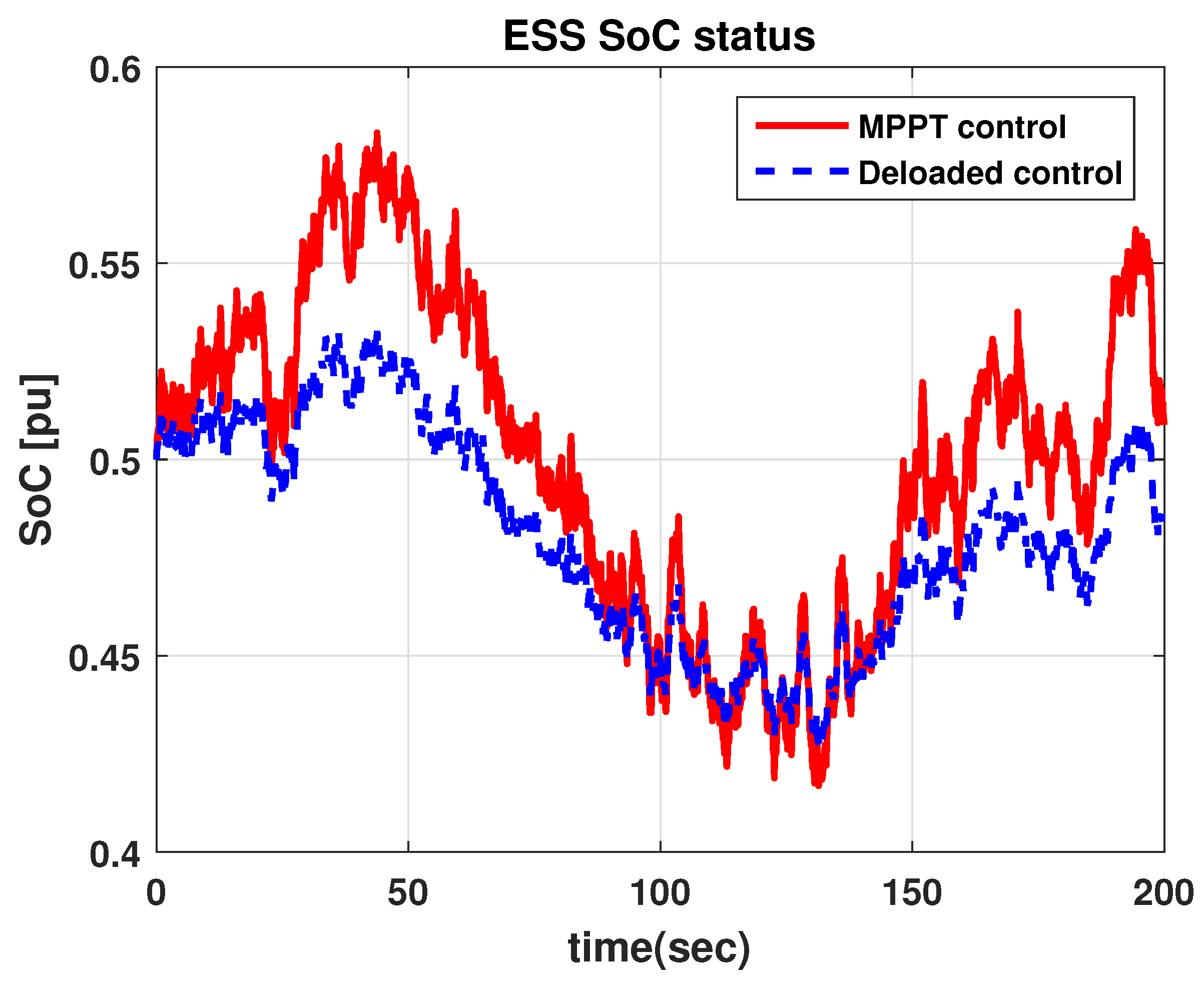
Figure 8.
Comparison of the power system frequency.

Figure 9.
Wind power fluctuation with different control algorithms when average wind speed is 10 m/s.
Figure 9.
Wind power fluctuation with different control algorithms when average wind speed is 10 m/s.

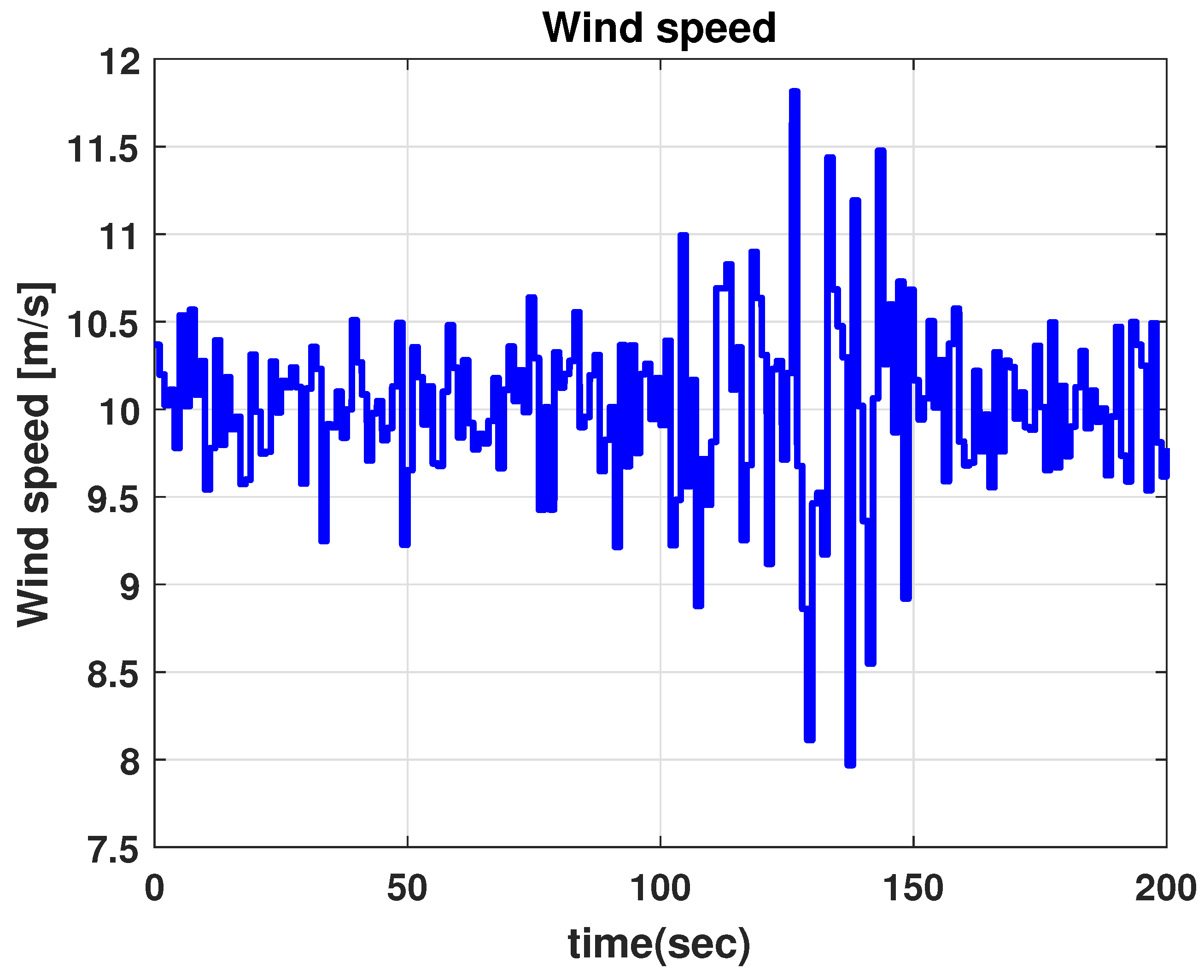
Figure 10.
Wind speed profile for the simulation when average wind speed is 10 m/s (sudden wind speed variation from 100 s to 150 s).
Figure 10.
Wind speed profile for the simulation when average wind speed is 10 m/s (sudden wind speed variation from 100 s to 150 s).

Figure 11.
Wind power fluctuation with different control algorithms when average wind speed is 10 m/s (sudden wind speed variation from 100 s to 150 s).
Figure 11.
Wind power fluctuation with different control algorithms when average wind speed is 10 m/s (sudden wind speed variation from 100 s to 150 s).

Figure 12.
Comparison of the ESS SoC for the different methods when average wind speed is 10 m/s (sudden wind speed variation from 100 s to 150 s).
Figure 12.
Comparison of the ESS SoC for the different methods when average wind speed is 10 m/s (sudden wind speed variation from 100 s to 150 s).
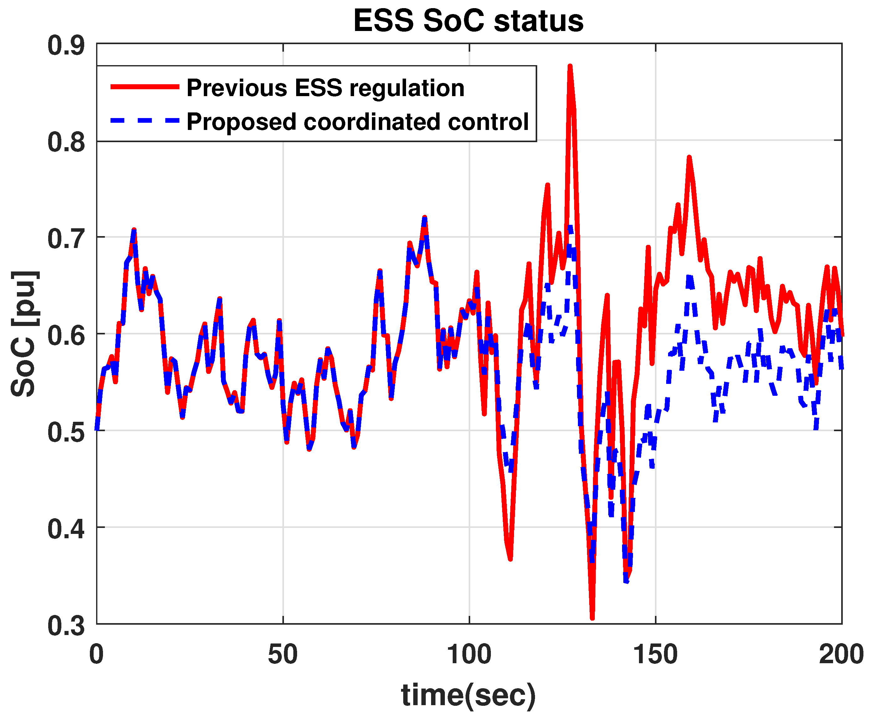
Figure 13.
Comparison of the power system frequency when average wind speed is 10 m/s (sudden wind speed variation from 100 s to 150 s).
Figure 13.
Comparison of the power system frequency when average wind speed is 10 m/s (sudden wind speed variation from 100 s to 150 s).
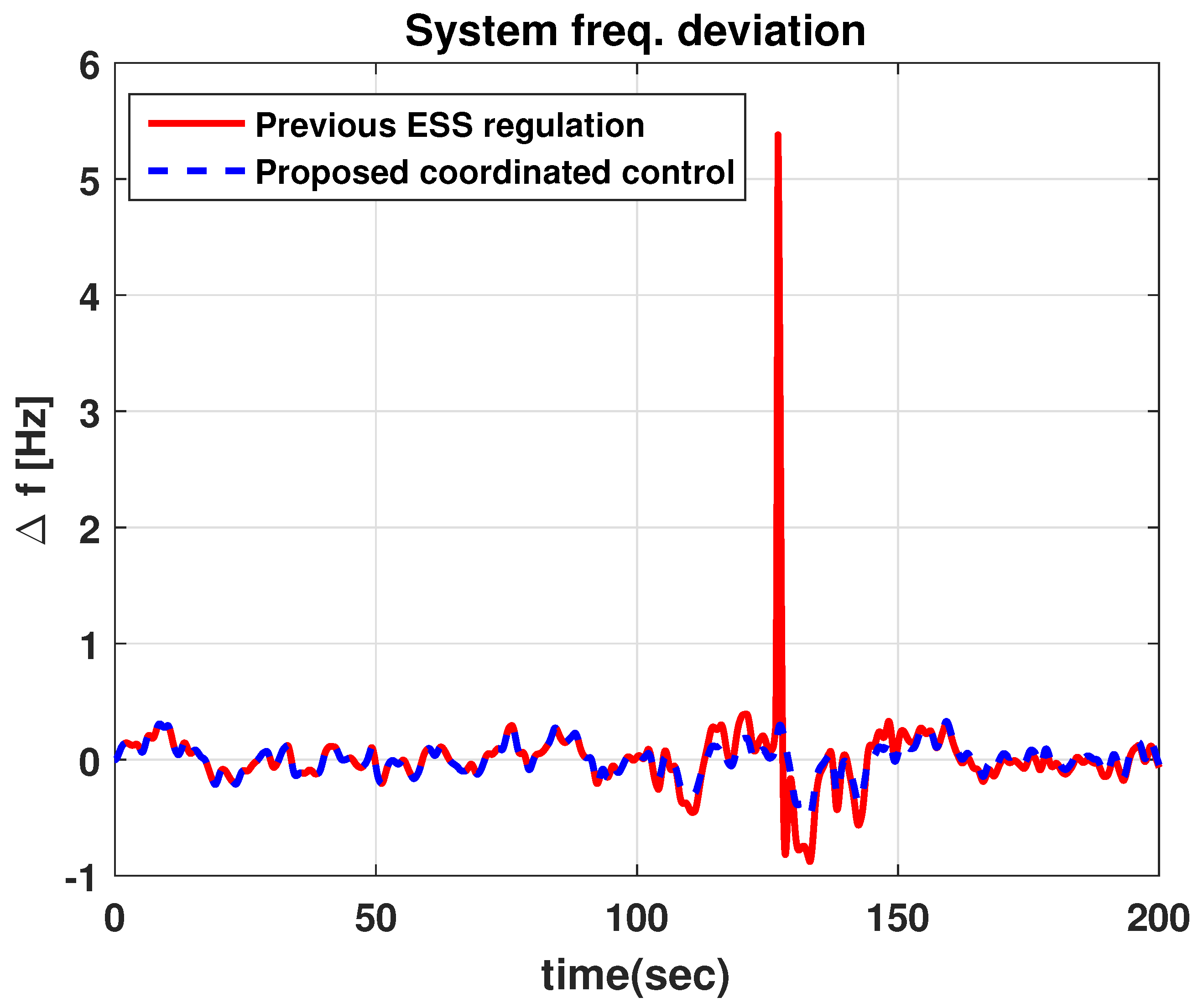
Figure 14.
Wind speed profile for the simulation when average wind speed is 13 m/s (sudden wind speed variation from 100 s to 150 s).
Figure 14.
Wind speed profile for the simulation when average wind speed is 13 m/s (sudden wind speed variation from 100 s to 150 s).

Figure 15.
Wind power fluctuation with different control algorithms when average wind speed is 13 m/s (sudden wind speed variation from 100 s to 150 s).
Figure 15.
Wind power fluctuation with different control algorithms when average wind speed is 13 m/s (sudden wind speed variation from 100 s to 150 s).

Figure 16.
Comparison of the ESS SoC for the different methods when average wind speed is 13 m/s (sudden wind speed variation from 100 s to 150 s).
Figure 16.
Comparison of the ESS SoC for the different methods when average wind speed is 13 m/s (sudden wind speed variation from 100 s to 150 s).
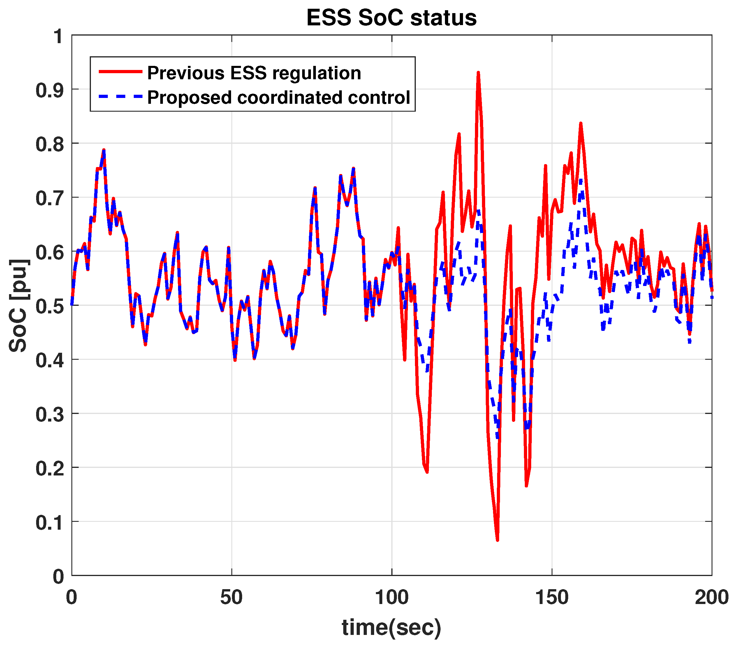
Figure 17.
Comparison of the power system frequency when average wind speed is 13 m/s (sudden wind speed variation from 100 s to 150 s).
Figure 17.
Comparison of the power system frequency when average wind speed is 13 m/s (sudden wind speed variation from 100 s to 150 s).
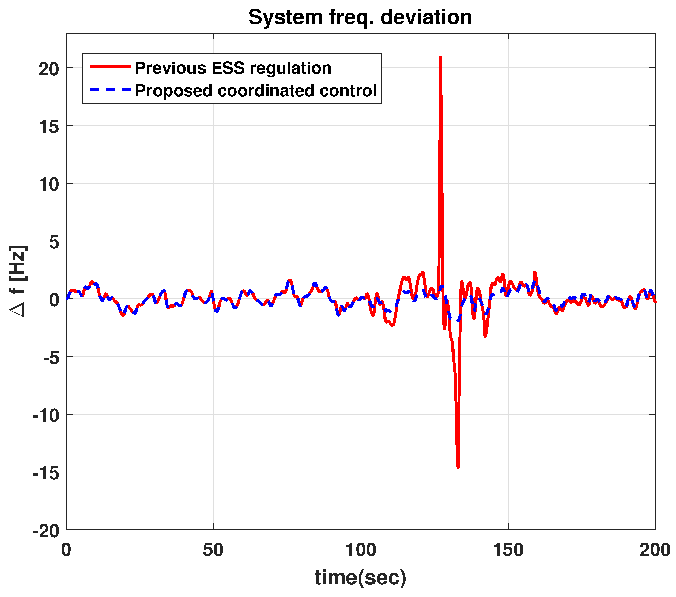
Figure 18.
Wind power fluctuations w/ and w/o consideration about ESS capacity in with reduced ESS capacity as 277 Wh when average wind speed is 13 m/s (sudden wind speed variation from 100 s to 150 s).
Figure 18.
Wind power fluctuations w/ and w/o consideration about ESS capacity in with reduced ESS capacity as 277 Wh when average wind speed is 13 m/s (sudden wind speed variation from 100 s to 150 s).
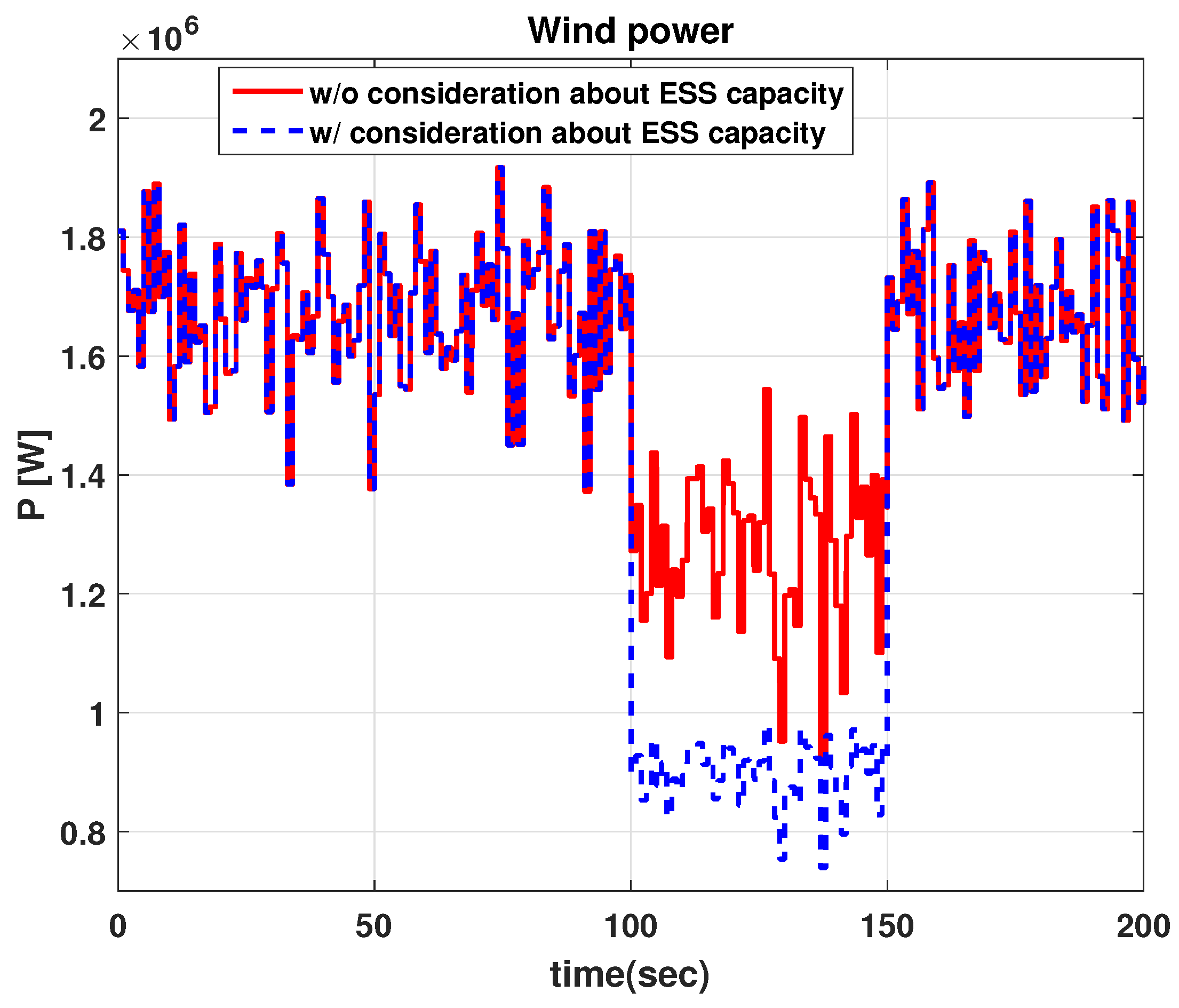
Figure 19.
Comparison of the ESS SoC w/ and w/o consideration about ESS capacity in with reduced ESS capacity as 277 Wh when average wind speed is 13 m/s (sudden wind speed variation from 100 s to 150 s).
Figure 19.
Comparison of the ESS SoC w/ and w/o consideration about ESS capacity in with reduced ESS capacity as 277 Wh when average wind speed is 13 m/s (sudden wind speed variation from 100 s to 150 s).
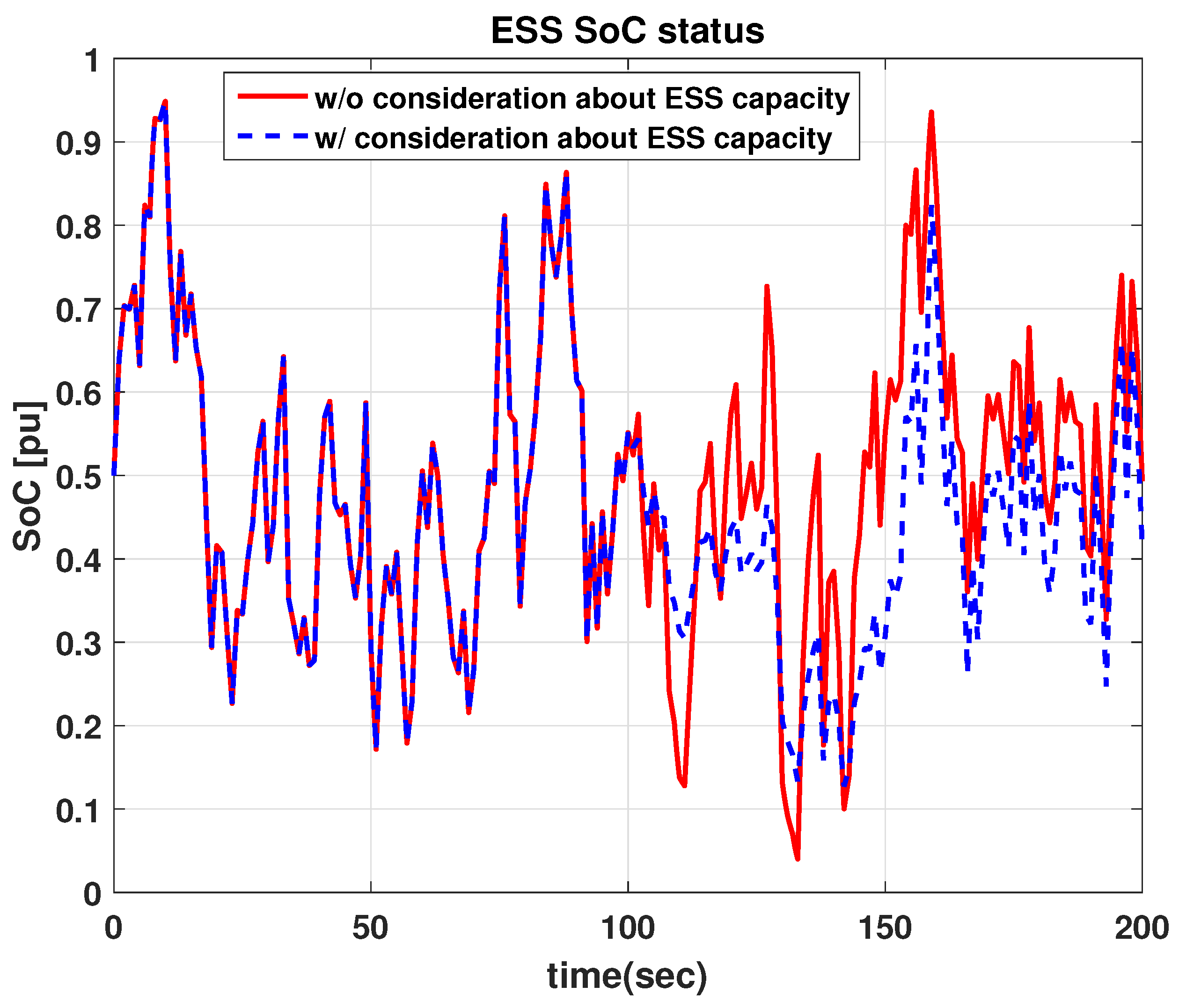
Figure 20.
Comparison of the power system frequency w/ and w/o consideration about ESS capacity in with reduced ESS capacity as 277 Wh when average wind speed is 13 m/s (sudden wind speed variation from 100 s to 150 s).
Figure 20.
Comparison of the power system frequency w/ and w/o consideration about ESS capacity in with reduced ESS capacity as 277 Wh when average wind speed is 13 m/s (sudden wind speed variation from 100 s to 150 s).

© 2017 by the authors. Licensee MDPI, Basel, Switzerland. This article is an open access article distributed under the terms and conditions of the Creative Commons Attribution (CC BY) license (http://creativecommons.org/licenses/by/4.0/).
Share and Cite
MDPI and ACS Style
Kim, C.; Muljadi, E.; Chung, C.C. Coordinated Control of Wind Turbine and Energy Storage System for Reducing Wind Power Fluctuation. Energies 2018, 11, 52. https://doi.org/10.3390/en11010052
AMA Style
Kim C, Muljadi E, Chung CC. Coordinated Control of Wind Turbine and Energy Storage System for Reducing Wind Power Fluctuation. Energies. 2018; 11(1):52. https://doi.org/10.3390/en11010052
Chicago/Turabian StyleKim, Chunghun, Eduard Muljadi, and Chung Choo Chung. 2018. "Coordinated Control of Wind Turbine and Energy Storage System for Reducing Wind Power Fluctuation" Energies 11, no. 1: 52. https://doi.org/10.3390/en11010052
Note that from the first issue of 2016, this journal uses article numbers instead of page numbers. See further details here.