H∞ Robust Control of an LCL-Type Grid-Connected Inverter with Large-Scale Grid Impedance Perturbation


1
School of Electrical and Power Engineering, China University of Mining and Technology, Xuzhou 221000, China
2
School of Information and Control Engineering, China University of Mining and Technology, Xuzhou 221000, China
*
Author to whom correspondence should be addressed.
Energies 2018, 11(1), 57; https://doi.org/10.3390/en11010057
Submission received: 15 November 2017
/
Revised: 10 December 2017
/
Accepted: 22 December 2017
/
Published: 1 January 2018
(This article belongs to the Section I: Energy Fundamentals and Conversion)
Abstract
:In the distributed power generation system (DPGS), there may be a large range perturbation values of equivalent grid impedance at the point of common coupling (PCC). Perturbation of the impedance will cause resonant frequency variation of the Inductance Capacitance Inductance (LCL) filter on a large scale, affecting the quality of the grid current of the grid-connected inverter (GCI) and even causing resonance. To deal with this problem, a novel H∞ robust control strategy based on mixed-sensitivity optimization is proposed in this paper. Its generalized controlled object is augmented by properly selecting weighting functions in order to consider both tracking performance around power frequency and the stability margin in a high frequency of the GCI. For convenient implementation, the H∞ robust controller is simplified by model reduction from the seventh order to the third order. By comparison with a traditional control strategy with a quasi-proportional resonance controller, the proposed H∞ robust control strategy avoids crossing 180 degrees at the resonant frequency point in the phase frequency characteristic of current loop, and moves the phase frequency characteristic left. It guarantees a sufficient margin of stability throughout the designed range of grid impedance perturbation values and avoids the difficulty of parameter setting. Finally, the experimental results support the theoretical analyses and demonstrate the feasibility of the proposed strategy.
1. Introduction
The distributed power generation system (DPGS) with renewable energy sources is becoming a promising power generation system which can improve efficiency and enhance the reliability of the power supply. Grid-connected inverters (GCIs) are broadly used as important interface devices between renewable energy generations and the grid [1].
When GCIs are connected in parallel at the point of common coupling (PCC), these GCIs will interact with each other for grid impedance, while the impact of grid impedance on these GCIs will increase by N times (N is the number of these GCIs) [2]. The grid-connected/islanded modes of GCIs will also frequently change the equivalent grid impedance in DPGSs [3]. With the increase of the penetration rate of GCIs, large-range perturbation of the equivalent grid impedance on the PCC may occur more and more frequently, and weaken the control performance of GCIs in DPGSs. The effects of grid impedance perturbation are shown in following aspects: (1) It can cause the resonant frequency variation of Inductance Capacitance Inductance (LCL) filter usually used as the output filter of GCI, and resonance even may occur; and (2) it will make the PCC voltage more sensitive and affect the quality of the grid current [4].
Due to sampling delay, modulation delay etc. in the current loop, stability cannot be ensured without suppressing the influence of grid impedance perturbation when fr (the resonant frequency of the LCL filter) is out of the range of [fs/4, fs/2] (fs is sampling frequency of GCIs), due to grid impedance perturbation [5,6,7]. To reduce the effect of grid impedance on the stability of GCIs, numerous methods have been proposed. The authors of [8,9] propose an impedance shaping method to change the output impedance characteristics of GCIs to improve the performance and robustness. The authors of [10] propose gain-scheduling adaptive control for suppressing the effect of grid impedance. A full feed-forward scheme of grid voltage presented by [11,12] is not suitable for the weak grid, which eliminates the influence of grid voltage on the grid current. To improve adaptability under a weak grid, a fundamental grid voltage feed-forward scheme with a harmonic resonance controller is proposed in [13]. However, as the grid-inductive impedance increases, the low frequency gain and bandwidth of the traditional control methods mentioned above have to be decreased to keep the system stable, thus degrading the tracking performance and disturbance rejection capability [14]. The authors of [15,16,17] manifest that the capacitor current feedback, as a widely used active damping method, cannot ensure the stability of the GCI and its sideband when fr is at fs/6.
Owing to the advantages of robust control strategy under parameter uncertainty, some methods [18,19,20] based on robust control theory have been applied to GCIs in recent years. Gabe et al. [18] describe the design and implementation of a robust controller using partial state feedback due to grid impedance uncertainty. In addition, an affiliated internal model controller is added to ensure reference tracking performance in this paper, which increases the complexity of control. Based on H∞ loop-shaping theory, a discrete robust controller in the d-q frame considering grid impedance perturbation is proposed in [19]. This method needs an additional active damping loop to suppress LCL filter resonance. Based on structured singular value (μ) minimization, a robust single-loop current control scheme is presented in [20], which has no use for an additional active loop. However, the controller designed by the robust control method is usually of a higher order, so it is difficult to implement in the actual GCI.
Firstly, a novel H∞ robust control strategy based on mixed-sensitivity optimization is proposed in the frame in this paper, in which the generalized controlled object is augmented by properly selecting weighting functions. For convenient implementation, a simplified third-order H∞ robust controller is further obtained by model reduction. Then, the proposed H∞ robust control strategy is analyzed by comparison with the tradition control strategy with a quasi-proportional resonance (PR) controller. The superiority of the proposed method is shown, as the proposed H∞ robust control strategy can suppress the resonance caused by large-scale grid impedance perturbation and guarantee good tracking performance at the same time. Moreover, the feasibility of controller simplification is demonstrated. Finally, the feasibility and superiority of the proposed H∞ robust strategy is proven through experiments.
The rest of this paper is organized as follows. In Section 2, the design and implementation of the H∞ robust controller are presented. Stability analysis of the proposed H∞ robust current control and traditional control strategy is presented in Section 3. In Section 4, the superiority of proposed H∞ robust control strategy in comparison with the traditional control strategy with the quasi-PR controller is proven through experiments. Finally, Section 5 concludes the paper.
2. Design of the H∞ Robust Current Controller Based on Mixed-Sensitivity Optimization
2.1. Modeling of the System
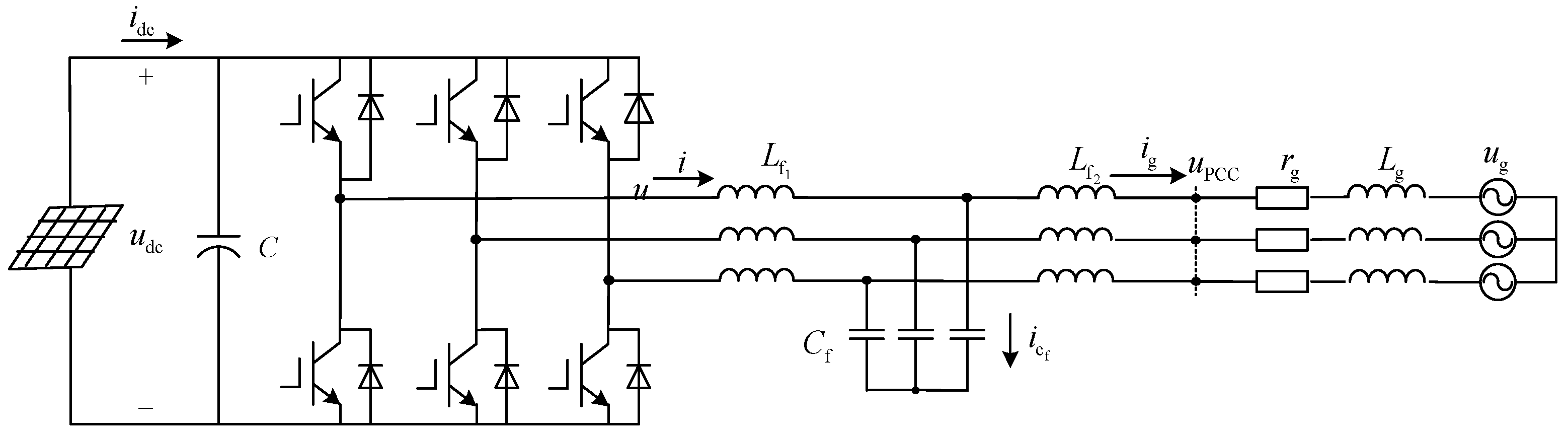
The circuit topology of GCI is shown as Figure 1, where Lf1 is an inverter-side inductor of the LCL filter; Lf2 is a grid-side inductor of the LCL filter; and Cf is the capacitor of the LCL filter. Zg = rg + jLg denotes equivalent grid impedance, including equivalent grid resistance and inductance. C is the direct current (DC) capacitor.
According to Kirchhoff’s voltage law (KVL) and Kirchhoff’s current law (KCL), the space state equations of GCI in the α–β frame are presented as (1).
where
To deal with the stability problem caused by grid impedance perturbation, a novel H∞ robust current controller based on mixed-sensitivity optimization is proposed in this paper. A standard H∞ model of GCI is built, as shown in Figure 2. The standard H∞ model of GCI is introduced as follows.
- (1)
- z donates the output signals to be minimized (with respect to both performance and robustness) which are named evaluation signals.
- (2)
- y represents the vectors of measurement available to the controller K(s), such as measurement outputs or tracking errors. In this system, because the main purpose of GCI is to control the output current, y = e = [iref − ig iref − ig]T is adopted.
- (3)
- w denotes external inputs of this system, for example disturbances, noises, references etc. While building the generalized controlled object P, grid voltages and current references are treated as disturbances, where r = [iref iref]T denotes current references, d = [ug ug]T denotes grid voltages, and w = [iref iref ug ug]T.
- (4)
- u denotes the output signals of the controller or input control signals of the system, namely the inverter side voltage of GCI, u = [u u]T.
- (5)
- P represents the generalized controlled object, including the original controlled object Gnom with nominal values of grid impedance and weighting functions W1, W2, W3 to match the control requirements of the design.
Based on Figure 1, the H∞ robust controller K is guaranteed to satisfy the control requirement of P’s output. According to Figure 2 and Equation (1), the space state equation of standard H∞ model is shown as follows.
where P denotes the augmented plant, I is the identity matrix, and W1, W2, W3 are weighting functions which will be presented in the following pages.
2.2. Design Parameters and Constraint Conditions of the Proposed H∞ Robust Controller
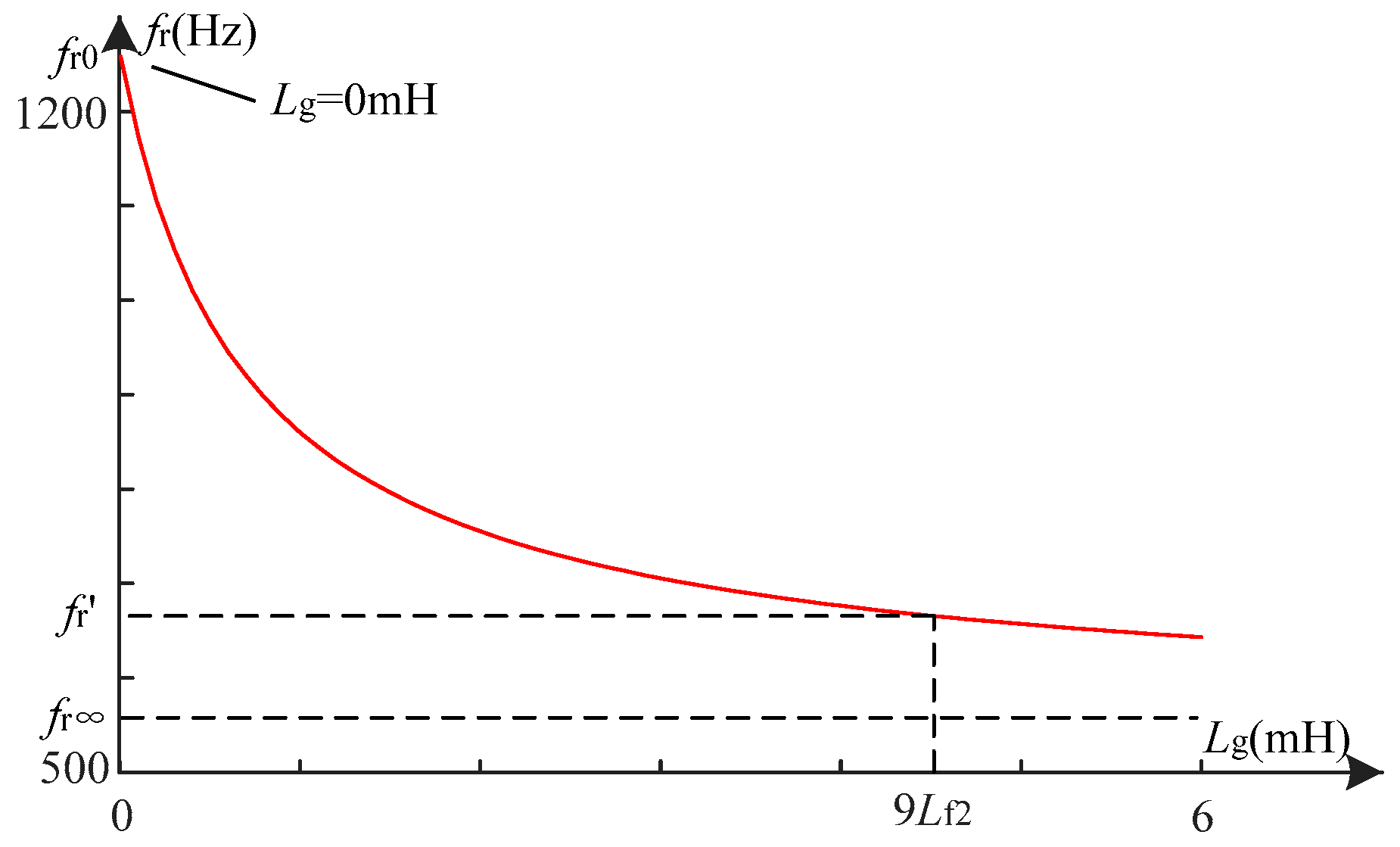
For the subsequent analysis and design, the parameters of this system are given in Table 1. For different grids, the values of grid impedance are different. It is difficult to obtain a specific range of grid impedance. However, with the impedance change, the limit of resonant frequency of the LCL-filter fr is determined. The equation with respect to fr and grid impedance is shown in (3). As shown in (3), the change of fr mainly depends on 1/((Lg + Lf2)Cf). When grid impedance tends to infinity, . Therefore, the fr value cannot be lower than that of fr∞.
H∞ robust controller is designed in order to suppress the resonance under a large range of grid impedance perturbation values. Hence, according to the change of the resonant frequency of the filter, the impedance perturbation range of the power grid is set up in this paper. The designed range of impedance perturbation values is set at 0–9Lf2, which makes 1/((Lg + Lf2)Cf in (3) negligible when Lg > 9Lf2, and the values are set as follows: Lf2 = 0.5 mH, and Lg changes from 0 mH to 4.5 mH. Figure 3 shows the resonant frequency change with grid impedance. The designed range covers most of the resonant frequency variations, and the grid impedance value is also large enough.
When solving the H∞ robust standard question, the generalized controlled object P must satisfy the following four conditions [21].
- (A, B2) is stabilizable and (C2, A) detectable;
- and , where m and p denote the rank of these unit matrices;
- has full column rank for all;
- has full row rank for all.
The goal of the H∞ robust controller is to minimize the H∞ norm from input w to output signals z, which means ||Twz||∞ < 1 or satisfies (4). S(s) = (1 + GnomK(s))−1 is the sensitivity function and T(s) = GnomK(s)(1 + GnomK(s))−1 is the complementary sensitivity function. They satisfy S(s) + T(s) = 1. R(s) = K(s)S(s).
Based on (4), S(s), T(s) and R(s) are obtained as (5), where donates the maximum singular value and donates the minimum singular value of the matrix [22]. S(s), T(s), and R(s) depend on the selection of weighting functions of W1, W2, and W3.
For explanations of (4) and (5) refer to the literature [23]. According to Figure 2, when grid voltages are not considered (d = 0) and the current references r are the only consideration, the relationships between the variables are shown (6).
When the grid voltages d are the only consideration (r = 0), the relationships between the variables are as shown in (7).
2.3. Design of Weighting Functions
Based on the above conditions, the design of the weighting functions is presented as follows.
(1) Weighting function W1
Based on (6), the error signal e depends on the sensitivity transfer function S. As r (current references) is a sinusoidal reference signal for power frequency, S(s) must have a high attenuation of power frequency to minimize the error. When the grid voltages d are the only consideration, mainly the influence of high-frequency disturbances is considered. According to (7), the output of t is only related to S(s), so high attenuation of W1 at high frequency is guaranteed to decrease the influence of grid voltages on the system.
According to (4), S(s) is restricted by 1/W1, which means the weighting function W1 should present a high gain in terms of power frequency and a high attenuation in high frequency. Therefore, the selection of W1 is as follows.
where ω0 = 100 is power frequency and determines the peak and bandwidth of W1, which shows a lower, narrower bandwidth as well as a greater peak. As this transfer function can achieve nearly zero error tracking [24], the attenuation of S(s) at power frequency can be treated as infinity.
(2) Weighting function W2
W2 cannot equal 0, and to satisfy ||W2R(s)||∞ ≤ 1, a small constant is chosen to obtain larger control signals u, W2 = 0.1.
(3) Weighting function W3
Multiplicative perturbation is adopted to describe the parameter uncertainty that the uncertainty branch Δ(s) is in parallel with forward path G. The description of multiplicative uncertainty is shown as.
G denotes the transfer function of the multiplicative perturbation system with grid impedance perturbing in predefined ranges, and Gnom denotes the transfer function of the system with nominal grid impedance Lgnom (shown in Table 1). For the predefined range of grid impedance perturbation values shown in Table 1, the original controlled object G contains uncertainty parameters. The singular values of multiplicative perturbation are shown in Figure 4, of which the green dashed lines are singular values of multiplicative perturbation with parameter uncertainty in the predefined range. At the same time, the red solid line represents singular values of multiplicative perturbation in the worst gain of the predefined perturbation range when Lg = 4.5 mH.
For multiplicative perturbation of the system, ||W3T(s)||∞ ≤ 1 in (4) must be satisfied. Therefore, the weighting function W3 should be designed for the worst gain in the predefined perturbation range to obtain the required robustness. The singular values of the designed weighting function are just above the worst gain in perturbation range. The singular value of W3 is above the singular value of multiplicative uncertainty Δ(s), which means that T(s) has high attenuation in high frequency from external input w to output signals z; it can reduce the effect of output disturbance at high frequency. In addition, for good reference tracking, T(s) should have no attenuation for the current references r. Thus, the synthesized controller can achieve high attenuation to restrain the effect of grid impedance perturbation. Furthermore, as S(s) + T(s) = 1, it is necessary to ensure that the crossover frequency of the magnitude response W1 at 0 dB is below the crossover frequency of the magnitude response of 1/W3 at 0 dB. This allows the controller to obtain a “gap” for the desired loop shape to pass between the performance bound W1 and robustness bound 1/W3. In the opposite case, the performance and robustness requirements will not be satisfied. W3 is chosen as in (10).
2.4. Synthesis and Analysis of the H∞ Robust Controller
The generalized controlled object P is augmented by the original controlled object Gnom, with weighting functions W1, W2, W3. By using the hinfsyn function of the MATLAB robust control toolbox [22], the H∞ robust controller K(s) based on mixed-sensitivity optimization is synthesized as (11).
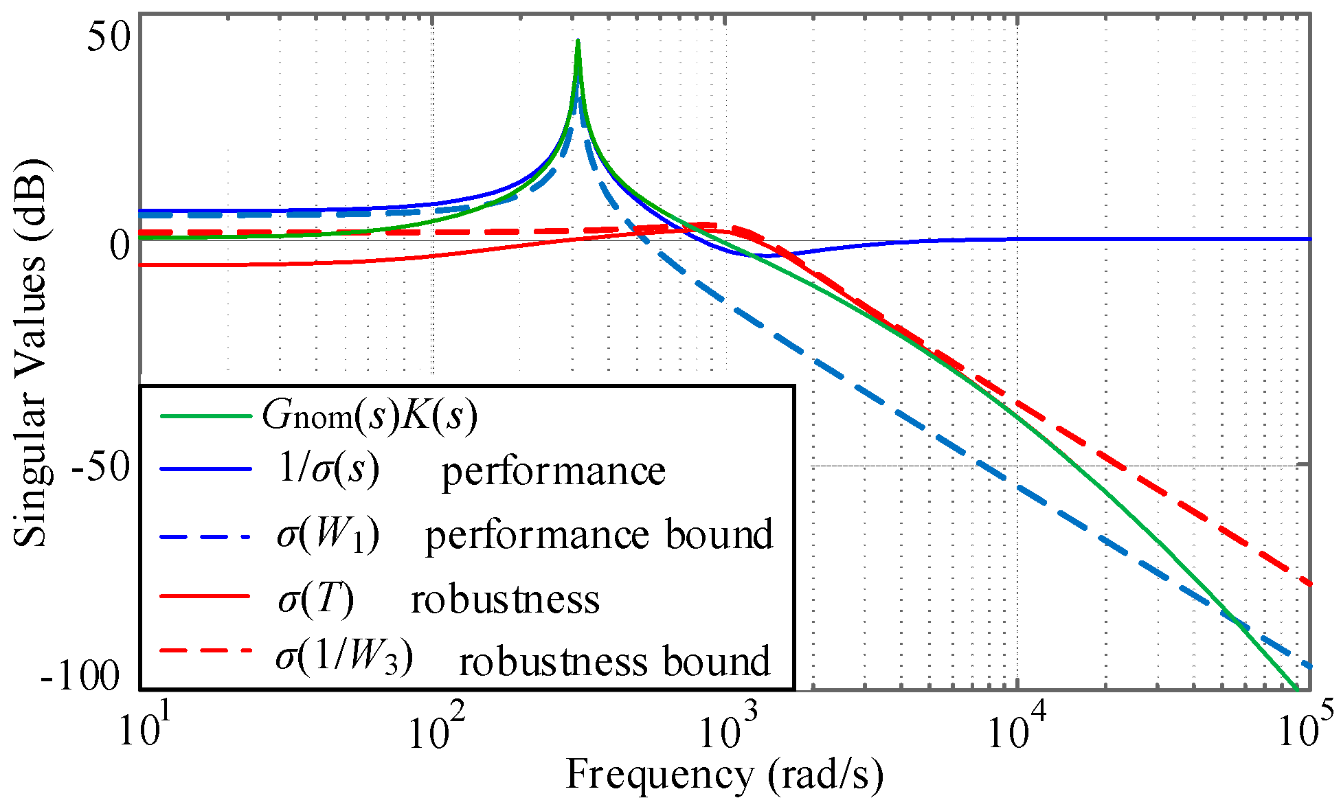
To obtain good performance and robustness, S(s), R(s), T(s) should satisfy (5). Figure 5 shows the singular values of S(s), T(s), W1, 1/W3, and GnomK(s). It is seen that (1/S) lies over (W1) and (T) is below (1/W3). Gnom(s) is on behalf of the singular value curve of the open loop transfer function of GCI robust control system, shown by the green solid line. The solid line represents the system characteristics at low and high frequencies. The solid line is located above the performance bound of W1 around the 50 Hz, and is located under the robustness bound of 1/W3 in the high frequency section. This proves that the transfer function characteristics meet the design performance and robustness. Both the performance and robustness can be obtained through the H∞ robust controller.
However, it is difficult to implement K(s) with a seventh-order controller in an actual GCI with a response time of only a few hundred microseconds. The discrete seventh-order controller needs six previous pieces of data which will cause six unknown variables at the start. It makes the start more difficult and may even cause the system to become out of control. Moreover, more multiplicative calculations and data registers are needed.
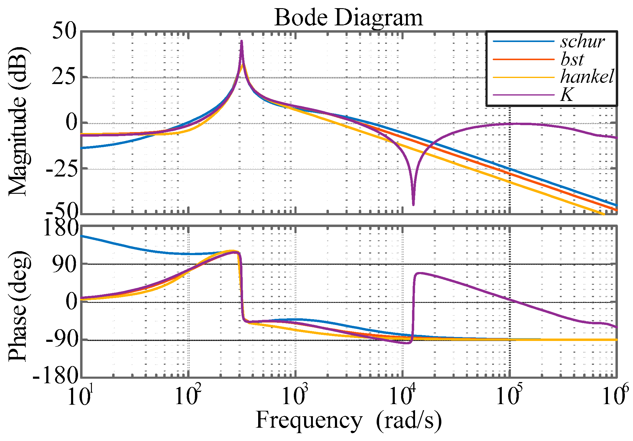
Hence, it is necessary to simplify the controller while maintaining most of the performance [21]. The selection principles of the order reduction are as follows: (1) Do not affect the performance of power frequency current control; and (2) Do not change the stability of the converter with the impedance perturbation. A Bode diagram of seventh-order controllers and the reduced third-order controllers by model reduction are shown in Figure 6. The reduced controller using the balance reduce strategy (the red solid line) is quite similar to the seventh-order controller and its error is lower than that found with controllers using the Schur strategy (the blue solid line) or Hankel strategy (the yellow solid line). The reduced controller using the balance reduce strategy can achieve the same control effect as K(s) in a low frequency range, and only change the magnitude characteristic in the high-frequency segment that has an effect on resonance. Such a change does not affect stability, and the reduced controller is the simplest, as shown in the analysis in Section 3.3. Hence, the reduced controller using the balance reduce strategy Kred(s) is chosen, as shown in (12).
where ω0 represents the angle frequency of the grid; here ω0 = 100π rad/s.
3. Stability Analysis of Proposed H∞ Robust Control and Traditional Control Strategy
3.1. Control Frame of LCL-Type Grid-Connected Inverter on Large-Scale Grid Impedance Perturbation
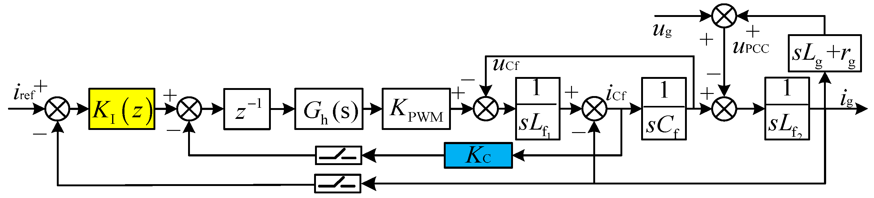
The frequently used control frame of the LCL-type GCI is shown in Figure 7. KC denotes the sampling coefficient of capacitor current feedback and KI(s) is current controller. KI(s) chooses Proportion Integration (PI) or quasi-PR in the traditional control strategy, and KC is added to the current loop as the active damping to suppress the resonance of the LCL filter. In the proposed H∞ robust controller, KI(s) is K(s) or Kred(s), and KC is not added, namely, KC = 0. z−1 is the one-sample computation delay. Gh(s) is a zero-order hold which is equivalent to the behavior of the Pulse Width Modulation (PWM) link, as shown in (13). Considering the influence of digital control, the open-loop transfer function of system in discrete domain is obtained by a discrete method of the sampling system, as shown in (14).
3.2. Stability Analysis under Traditional Control Strategy
For comparison with the proposed control strategy in the α–β frame, discrete quasi-PR [25] is preferred, as is shown in (15). As the bandwidth of quasi-PR is ωc/πHz and the allowed range of grid current is ±0.2 Hz, ωc = 1.257, kP = 3, and kR = 200.
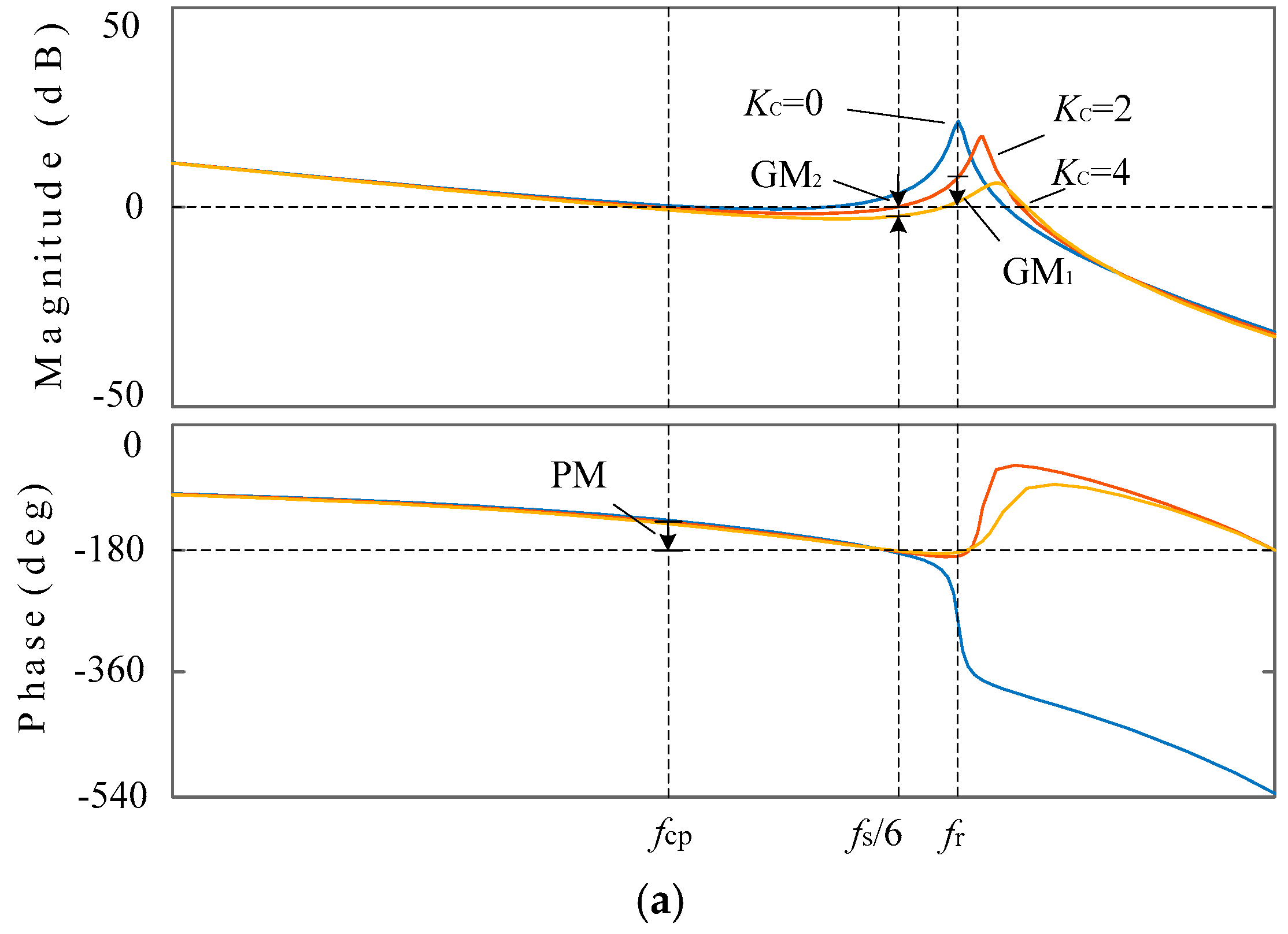
Equation (15) is put into (14), and an open-loop transfer function F(z) of the traditional control strategy is obtained. Figure 8 is a Bode diagram of F(z). The following stability analysis was obtained according to [16]. The size relation between fr and fs/6 is the key to judging the stability of the system with quasi-PR. GM1 and GM2 are defined as the magnitude margin of open-loop transfer function at fr and fs/6. PM = 180° + ϕ(ωc) is the phase margin of open-loop transfer function at cross-over frequency fc when the magnitude characteristic crosses 0 dB. In Figure 8, it is clearly shown that when KC = 0, regardless of the size of fr and fs/6, the system is not stable. When KC > 0, the analysis is as follows:
Situation (1): When fr > fs/6, the magnitude and phase characteristic of the open loop are as shown in Figure 8a. The phase characteristic negatively crosses −180° at fs/6 and positively crosses −180° at fr. To ensure system stability, GM1 < 0 dB, GM2 > 0 dB and PM > 0° should be satisfied. Hence, in Figure 8a, when KC = 2, the system is not stable.
Situation (2): When fr < fs/6, the magnitude and phase characteristic of the open loop are shown in Figure 8b. When the phase characteristic only negatively crosses −180° at fr, KC = 4, GM1 > 0 dB, and PM > 0° for example should be satisfied to ensure system stability. When the phase characteristic negatively crosses −180° at fr and positively crosses −180° at fs/6, KC = 2, GM1 > 0 dB, GM2 < 0 dB, and PM > 0° for example should be satisfied to ensure system stability, which is in contrast to Situation (1). Hence, in Figure 8b, when KC = 2, the system is also not stable.
Situation (3): When fr = fs/6, magnitude and phase characteristic of the open loop are as shown in Figure 8c. The phase characteristic is tangential to −180° at fr = fs/6, GM1 = GM2. At this time, regardless of whether GM1 and GM2 is larger or smaller than 0, the system stability cannot be guaranteed. Hence, in Figure 8c, when KC = 2 or KC = 4, the system is also not stable.
Hence, when designing the parameters of the LCL filter, the forbidden area is set up at fs/6 and its sideband to avoid fr from crossing fs/6 under the traditional control strategy. However, when considering grid impedance, fr is shown in (3). The grid impedance perturbation will lead to large-scale fluctuation of fr, so that it may cross or even equal fs/6, which leads to the KC parameter settings being difficult or impossible. Even if the sampling coefficient of capacitor current feedback is well designed according to fr > fs/6 or fr < fs/6, one parameter is not sure to meet the requirements at the same time. Hence, for the system with quasi-PR it is difficult to ensure stability with respect to large-scale grid impedance perturbation.
3.3. Stability Analysis under Proposed H∞ Robust Control Strategy
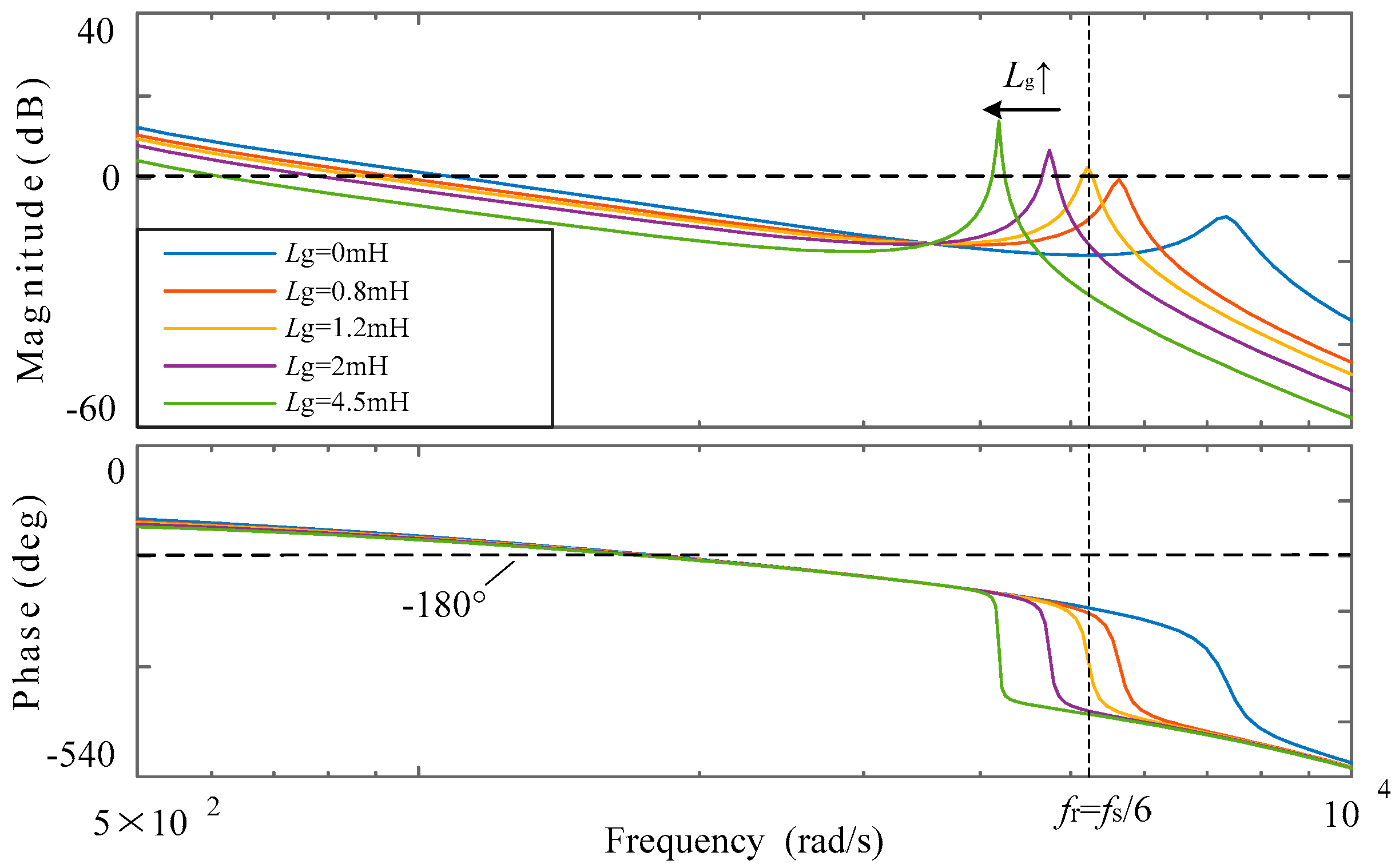
In the proposed H∞ robust control strategy, KI(s) is the H∞ robust controller K(s) or Kred(s), and capacitor current feedback is not added (KC = 0). To compare the traditional control strategy and the proposed H∞ robust control, a Bode diagram of open-loop transfer functions under the two strategies at fr = fs/6 is shown in Figure 9. The blue line is a Bode diagram of the open-loop transfer function under the traditional control strategy with a quasi-PR controller. When the phase characteristic is tangential to −180° at fr, GM = −29 dB. Based on the above analysis, regardless of whether the phase margin is larger or smaller than 0, the system stability cannot be guaranteed. The yellow line shows the open loop transfer function under the H∞ robust control strategy with the seventh-order controller K(s). The red line is a bode diagram of the open loop transfer function under the H∞ robust control strategy with the reduced third-order controller Kred(s). Both the system with the H∞ robust controller K(s) and with Kred(s) are stable at fr = fs/6, GM = 9.7 dB, PM = 48°. According to Figure 9, the H∞ robust controller moves across −180° of phase frequency characteristic left by decreasing phase margin to provide larger magnitude margin and avoid its crossing at the LCL resonant frequency. The system with the reduced third-order controller Kred(s) has a certain magnitude margin and phase margin in the range of grid impedance designed, shown in Figure 10.
According to (13), Kred(s) can be divided into an inertia link K1(s) and a second-order controller K2(s). Figure 11 is the bode diagram of Kred(s), K1(s) and K2(s). It is clearly seen that Kred(s) is mainly controlled by K2(s) around the power frequency. At a high frequency, the magnitude and phase characteristics of K2(s) are 0, which cannot attenuate the high frequency signals. Kred(s) is fully controlled by K1(s) in high frequency. Generally, the inertia link can be unified as (16), where T denotes the time constant. Figure 12 is the bode diagram of the open loop transfer function with the change of T. Large T will lead to small phase margin and high frequency gain. The inertia link leads to moves across −180° of phase frequency characteristic left to provide a certain magnitude margin, and ensure stability of the system under proposed H∞ robust control strategy on large scale grid impedance perturbation. Hence, the inertia link is added necessarily in the reduced controller and the third-order controller is the most simplified controller available.
4. Experimental Validation
According to the topology of GCI shown in Figure 1, an experimental platform is constructed as shown in Figure 13. The high-performance CompactRIO-9030 controller of the National Instruments Company is used as the core controller. The Model 62000H of Chroma Company is used to output DC voltage at the DC side. The inductances in series are adopted to simulate the grid impedance. In the AC side, an AC transformer is used to connect the grid. The leakage inductance of three-phase transformer is combined with the grid impedance. The parameters are shown in Table 1. Based on the parameters and the range of grid impedance perturbation given by Table 1, the experiment compares the proposed H∞ robust control strategy and quasi-PR control with capacitor current feedback. Because the leakage inductance of three-phase transformer is small, Lg = 0 mH actually means that GCI is only connected to the secondary side of the alternating current (AC) transformer instead of the inductances in series. The control frame of the GCI is shown in Figure 7.
Experimental results of traditional control strategy with a quasi-PR controller on grid impedance perturbation are shown in Figure 14, and the total harmonic distribution (THD) of three-phase currents and PCC voltages are presented in Figure 15. At time t1, when Lg changes from 0 mH to 0.8 mH, fr > fs/6. The THD of grid-side currents increases from 2.7 to 5.7% while the THD of PCC voltages increases from 3.2 to 6.2%. At this moment, the distortion of currents and PCC voltages occurs. The system still maintains stable and resonance is avoided. At time t2, when Lg changes from 0.8 mH to 1.2 mH, fr = fs/6. The whole system becomes resonant and the quality of currents decreases clearly, as well as the PCC voltages. The experimental results manifest that when grid impedance perturbs (fr crossing fs/6), the system under traditional control strategy becomes unstable.
Figure 16 shows the experimental results under the proposed H∞ robust control strategy, while Figure 17 shows THD of the three-phase currents and PCC voltages under the proposed H∞ robust control strategy. In Figure 16, after Lg suddenly changes from 0 mH to 0.8 mH at t1, the proposed H∞ robust controller can ensure the inverter is stable when THD of its currents is 3.3% and the THD of its PCC voltages is 3.2%. When Lg suddenly changes from 0.8 mH to 1.2 mH at t2, fr = fs/6, and the system is still stable. Furthermore, because the nominal value of the grid impedance (Lgnom = 1.2 mH) is adopted when the proposed H∞ robust controller is synthesized, the control effect is best in this nominal value, which is consistent with the experimental results in Figure 17. When Lg suddenly changes from 1.2 mH to 4.5 mH (fr→fr∞) at t3, the system keeps still stable. After t3, the THDs of its currents and PCC voltages increase separately to 3.9% and 6.2% in Figure 17. The THD of the currents is within the allowable range. This experimental results manifest that the proposed robust control strategy can obtain better effect under the same conditions, as compared with the traditional control strategy. These experimental results are consistent with theoretical analysis above.
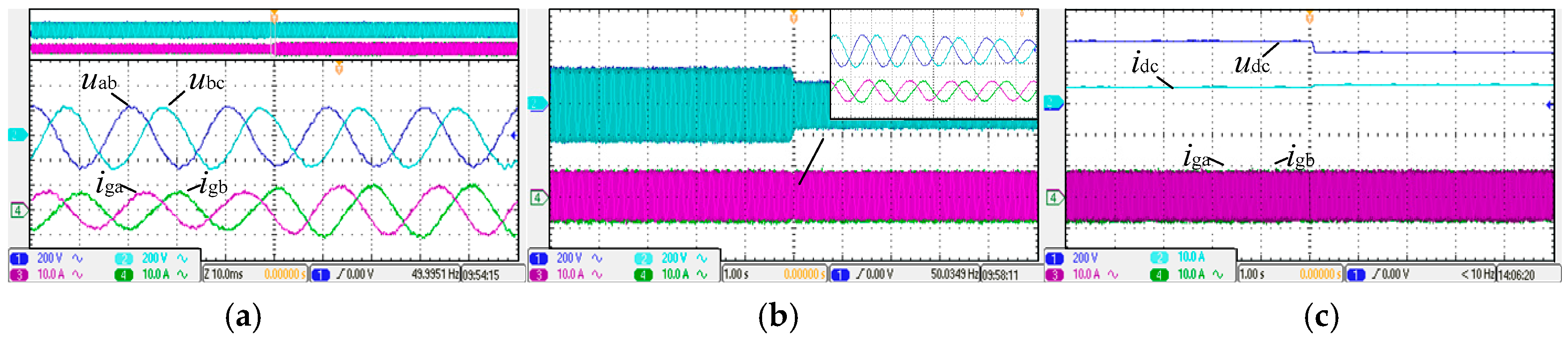
For further verification of the stability of the system with the proposed H∞ robust control strategy, the experimental results under the several conditions (three-phase current stepping, PCC voltage dropping and DC voltage dropping) are shown in Figure 18. Lg is 4.5 mH in this experiment. When the current reference iref increases from 9 A to 11 A, the factual three-phase currents can fleetly track the reference, shown in Figure 18a. When PCC line voltage ugab drops from 190 V to 120 V, the three-phase currents can still remain stable, as shown in Figure 18b. When DC voltage udc drops from 400 V to 330 V, the output current at DC side jumps from 5 A to 6 A to ensure the output power is stable. The magnitude of the three-phase currents can keep invariant, as shown in Figure 16c.
5. Conclusions
This paper proposes a novel H∞ robust control strategy based on mixed-sensitivity optimization in a stationary frame and illustrates the specific design steps. It gives a comparative analysis with a traditional control strategy with a quasi-PR controller. When the fr of LCL filter does not equal fs/6, with the change of grid impedance, a good magnitude and phase margin can be guaranteed to ensure system stability under the traditional control strategy by properly selecting the several sampling coefficients of capacitor current feedback. However, one coefficient may not simultaneously meet the requirements in the two ranges of fr > fs/6 and fr < fs/6. When the fr of the LCL filter equals fs/6 due to the grid impedance perturbation, the phase characteristic is tangential to −180°. The traditional control strategy cannot guarantee system stability no matter how it is designed. When the proposed H∞ robust controller is adopted, the reduced controller actually contains a second-order controller and an inertia link. The second-order controller achieves tracking performance without a steady-state error around power frequency. The inertia link moves −180° left of the phase frequency characteristic to increase magnitude margin, and guarantees the system stability in large-scale grid impedance perturbation.
The superiority of the proposed control strategy is summarized as follows: (1) Single-loop current feedback control is applied to control GCI with inherent damping of LCL filter resonance instead of adding an active damping loop; (2) Capacitor current sensors are not needed, which reduces the numbers of sensors; (3) The proposed H∞ robust controller has characteristics of high gain at the power frequency and its sideband, and has a sufficient margin of stability in high frequency, which can guarantee good tracking performance and inhibit resonance throughout the designed range of grid impedance perturbation; and (4) The H∞ robust controller is simplified to the third order, which is more suitable for implementation.
Acknowledgments
The authors gratefully acknowledge the support provided by the Fundamental Research Funds for the Central Universities (2017XKQY029).
Author Contributions
Yingjie Wang and Jiashi Wang design the research; Wei Zeng and Haiyuan Liu collected and compiled the data and literature; Yingjie Wang and Yushuo Chai finished the experiment and calculation; Yingjie Wang and Jiashi Wang analyzed the results and put forward the policies. All authors read and approved the final manuscript.
Conflicts of Interest
The authors declare no conflict of interest.
References
- Blaabjerg, F.; Teodorescu, R.; Liserre, M.; Timbus, A.V. Overview of Control and Grid Synchronization for Distributed Power Generation Systems. IEEE Trans. Ind. Electron. 2006, 53, 1398–1409. [Google Scholar] [CrossRef]
- Agorreta, J.L.; Borrega, M.; LóPez, J.; Marroyo, L. Modeling and Control of N-Paralleled Grid-Connected Inverters with LCL Filter Coupled Due to Grid Impedance in PV Plants. IEEE Trans. Power Electron. 2011, 26, 770–785. [Google Scholar] [CrossRef]
- Cobreces, S.; Bueno, E.; Rodriguez, F.J.; Huerta, F. Influence Analysis of the Effects of an Inductive-Resistive Weak Grid over L and LCL Filter Current Hysteresis Controllers. In Proceedings of the 2007 European Conference on Power Electronics and Applications, Alborg, Denmark, 2–5 September 2007; pp. 1–10. [Google Scholar]
- Xu, J.; Xie, S.; Tang, T. Evaluations of Current Control in Weak Grid Case for Grid-Connected LCL-filtered Inverter. IET Power Electron. 2013, 6, 227–234. [Google Scholar] [CrossRef]
- Zou, C.; Liu, B.; Duan, S.; Li, R. Influence of Delay on System Stability and Delay Optimization of Grid-Connected Inverters with LCL Filter. IEEE Trans. Ind. Inform. 2014, 10, 1775–1784. [Google Scholar] [CrossRef]
- Lyu, Y.; Lin, H.; Cui, Y. Stability Analysis of Digitally Controlled LCL-type Grid-Connected Inverter Considering the Delay Effect. IET Power Electron. 2015, 8, 1651–1660. [Google Scholar] [CrossRef]
- Wang, J.; Yan, J.D.; Jiang, L.; Zou, J. Delay-Dependent Stability of Single-Loop Controlled Grid-Connected Inverters with LCL Filters. IEEE Trans. Power Electron. 2016, 31, 743–757. [Google Scholar] [CrossRef]
- Yang, D.; Ruan, X.; Wu, H. Impedance Shaping of the Grid-Connected Inverter with LCL Filter to Improve its Adaptability to the Weak Grid Condition. IEEE Trans. Power Electron. 2014, 29, 5795–5805. [Google Scholar] [CrossRef]
- Yang, D.; Ruan, X.; Wu, H. Using Virtual Impedance Network to Improve the Control Performances of LCL-Type Grid-Connected Inverter under the Weak Grid Condition. In Proceedings of the 2014 Twenty-Ninth Annual IEEE Applied Power Electronics Conference and Exposition, Fort Worth, TX, USA, 16–20 March 2014; pp. 3048–3054. [Google Scholar]
- Cespedes, M.; Sun, J. Adaptive Control of Grid-Connected Inverters Based on online Grid Impedance Measurements. IEEE Trans. Sustain. Energy 2014, 5, 516–523. [Google Scholar] [CrossRef]
- Xue, M.; Zhang, Y.; Kang, Y.; Yi, Y.; Li, S.; Liu, F. Full Feed forward of Grid Voltage for Discrete State Feedback Controlled Grid-Connected Inverter with LCL Filter. IEEE Trans. Power Electron. 2012, 27, 4234–4247. [Google Scholar] [CrossRef]
- Li, W.; Ruan, X.; Pan, D.; Wang, X. Full-Feedforward Schemes of Grid Voltages for a Three-Phase LCL-Type Grid-Connected Inverter. IEEE Trans. Ind. Electron. 2013, 60, 2237–2250. [Google Scholar] [CrossRef]
- Xu, J.; Qian, Q.; Xie, S.; Zhang, B. Grid-Voltage Feedforward Based Control for Grid-Connected LCL-Filtered Inverter with High Robustness and Low Grid Current Distortion in Weak Grid. In Proceedings of the 2016 IEEE Applied Power Electronics Conference and Exposition, Long Beach, CA, USA, 20–24 March 2016; pp. 1919–1925. [Google Scholar]
- Yang, S.; Lei, Q.; Peng, F.Z.; Qian, Z. A Robust Control Scheme for Grid-Connected Voltage-Source Inverters. IEEE Trans. Ind. Electron. 2011, 58, 202–212. [Google Scholar] [CrossRef]
- Chen, C.; Xiong, J.; Wan, Z.; Lei, J.; Zhang, K. A Time Delay Compensation Method Based on Area Equivalence for Active Damping of an LCL-Type Converter. IEEE Trans. Power Electron. 2017, 32, 762–772. [Google Scholar] [CrossRef]
- Pan, D.; Ruan, X.; Bao, C.; Li, W. Capacitor current feedback Active Damping with Reduced Computation Delay for Improving Robustness of LCL-Type Grid-Connected Inverter. IEEE Trans. Power Electron. 2014, 29, 3414–3427. [Google Scholar] [CrossRef]
- Bao, C.; Ruan, X.; Wang, X.; Li, W. Step-by-Step Controller Design for LCL-Type Grid-Connected Inverter with Capacitor–Current-Feedback Active-Damping. IEEE Trans. Power Electron. 2014, 29, 1239–1253. [Google Scholar]
- Gabe, I.J.; Montagner, V.F.; Pinheiro, H. Design and Implementation of a Robust Current Controller for VSI Connected to the Grid through an LCL Filter. IEEE Trans. Power Electron. 2009, 24, 1444–1452. [Google Scholar] [CrossRef]
- Cobreces, S.; Bueno, E.J.; Rodriguez, F.J.; Pizarro, D.; Huerta, F. Robust Loop-shaping H∞ Control of LCL-connected Grid Converters. In Proceedings of the 2010 IEEE International Symposium on Industrial Electronics, Bary, Italy, 4–7 July 2010; pp. 3011–3017. [Google Scholar]
- Kahrobaeian, A.; Mohamed, Y.A.I. Robust Single-Loop Direct Current Control of LCL-Filtered Converter-Based DG Units in Grid-Connected and Autonomous Microgrid Modes. IEEE Trans. Power Electron. 2014, 29, 5605–5619. [Google Scholar] [CrossRef]
- Huang, X.; Zhang, H.; Zhang, G.; Wang, J. Robust Weighted Gain-Scheduling H-Infinity Vehicle Lateral Motion Control with Considerations of Steering System Backlash-Type Hysteresis. IEEE Trans. Control Syst. Technol. 2014, 22, 1740–1753. [Google Scholar] [CrossRef]
- Li, W.K.; Zhou, G.; Chen, Y.B.; Gao, J.D. GA Optimized Signal Based Mixed Sensitivity Controller Design for Ship Heading Changing. In Proceedings of the 2015 Chinese Automation Congress, Wuhan, China, 27–29 November 2015; pp. 179–182. [Google Scholar]
- Gu, D.W.; Petkov, P.H.; Konstantinov, M.M. Robust Control Design with MATLAB®; Advanced Textbooks in Control & Signal Processing; Springer: Berlin, Germany, 2005. [Google Scholar]
- Komurcugil, H.; Altin, N.; Ozdemir, S.; Sefa, I. Lyapunov-Function and Proportional-Resonant-Based Control Strategy for Single-Phase Grid-Connected VSI with LCL Filter. IEEE Trans. Ind. Electron. 2016, 63, 2838–2849. [Google Scholar] [CrossRef]
- Yepes, A.G.; Freijedo, F.D.; Gandoy, J.D.; Lopez, O.; Malvar, J.; Comesana, P.F. Effects of discretization methods on the performance of resonant controllers. IEEE Trans. Power Electron. 2010, 25, 1692–1712. [Google Scholar] [CrossRef]
Figure 1.
Topology of a grid-connected inverter (GCI) with an Inductance Capacitance Inductance (LCL) filter and grid impedance.
Figure 1.
Topology of a grid-connected inverter (GCI) with an Inductance Capacitance Inductance (LCL) filter and grid impedance.

Figure 2.
Standard H∞ model of a GCI.
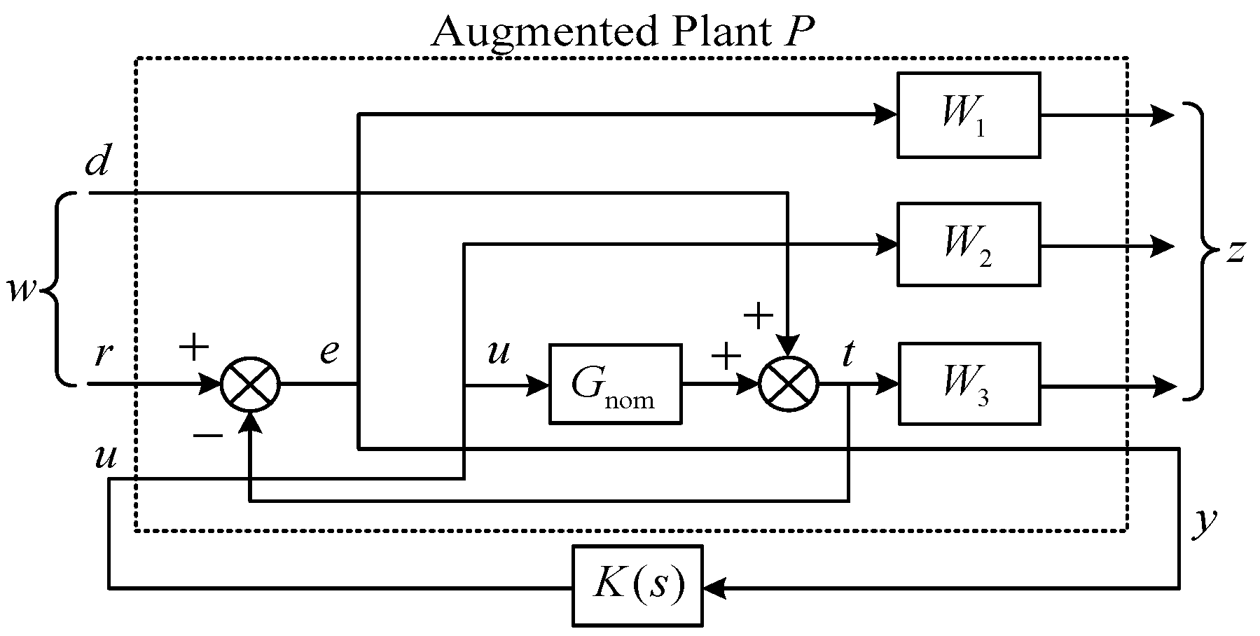
Figure 3.
Resonant frequency change with grid impedance.

Figure 4.
Description of multiplicative perturbation.
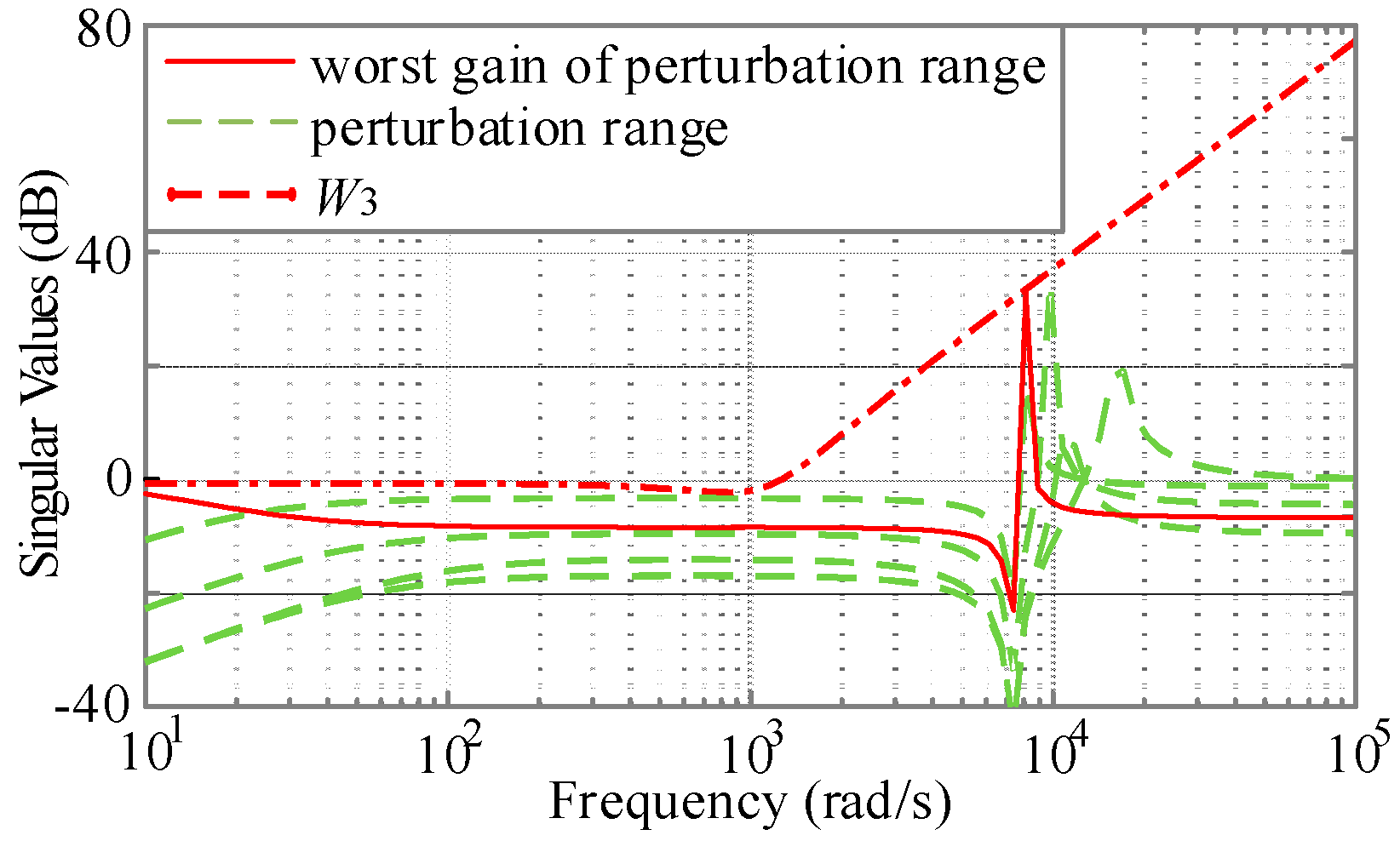
Figure 5.
Singular values of the open-loop system.

Figure 6.
Bode diagram of the seventh-order controller and the reduced controllers.

Figure 7.
Control frame of the LCL-type GCI. PWM: Pulse Width Modulation

Figure 8.
Bode diagram of F(z) with quasi-PR. (a) fr > fs/6, (b) fr < fs/6, (c) fr < fs/6.

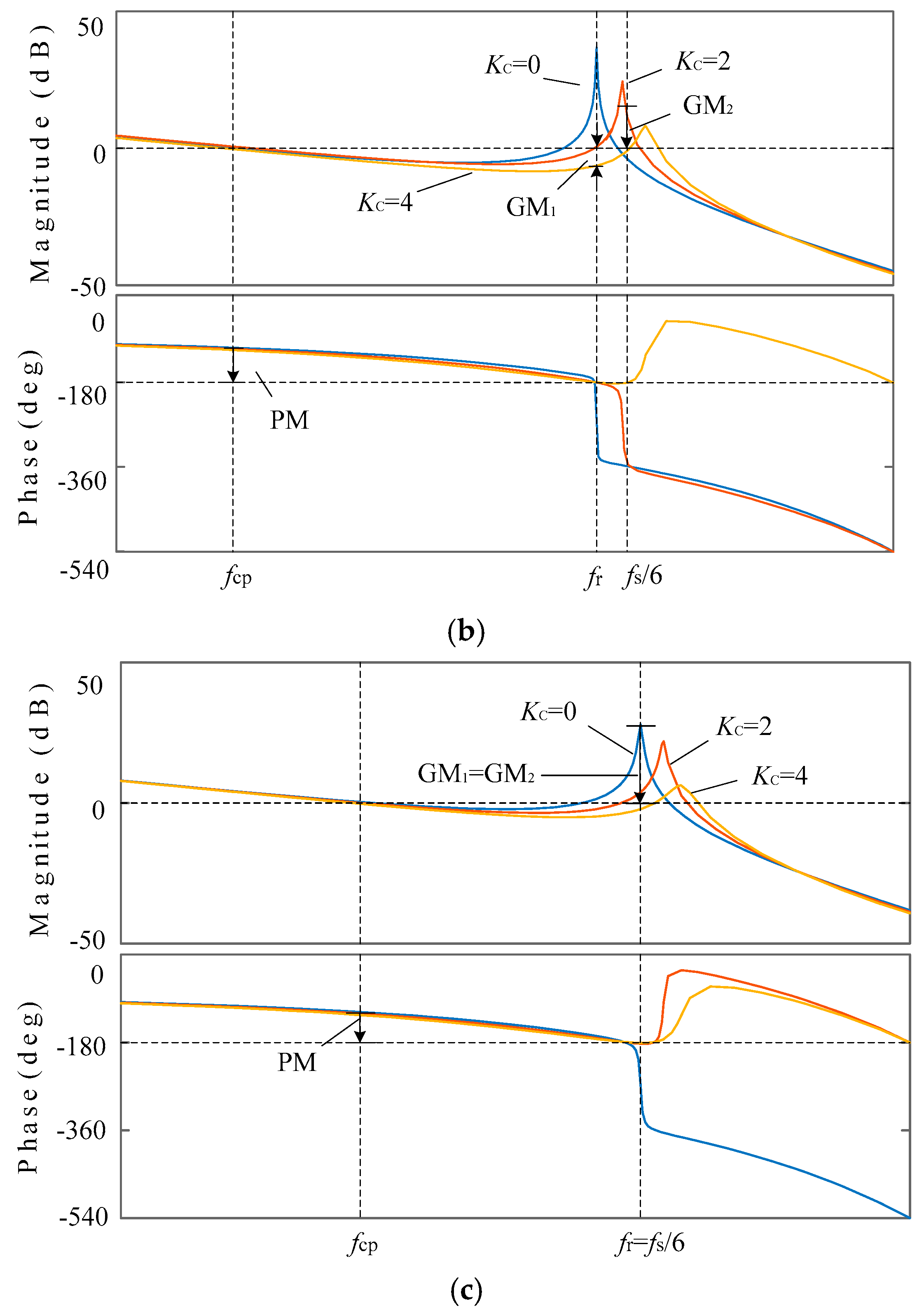
Figure 9.
Bode diagram of open-loop system with quasi-PR, Kred(s) and K(s).
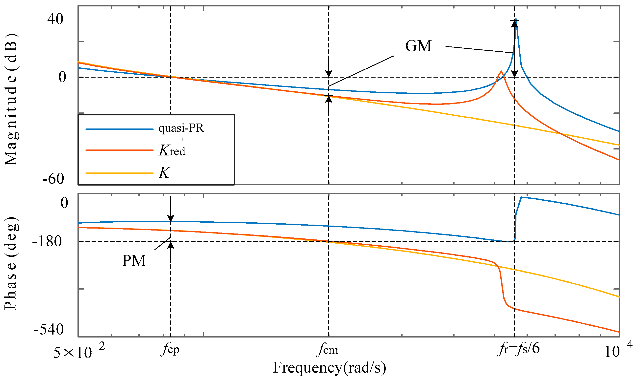
Figure 10.
Bode diagram of open-loop system with Kred on large scale grid impedance perturbation.

Figure 11.
Bode diagram of Kred(s), K1(s), K2(s).
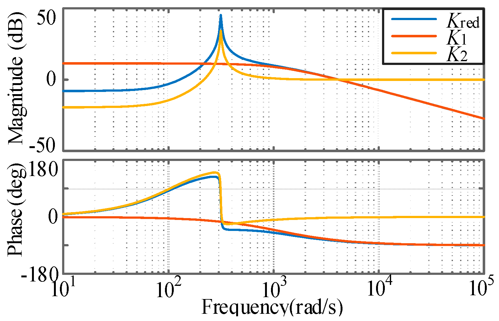
Figure 12.
Bode diagram of open-loop system with different T of K1(s).
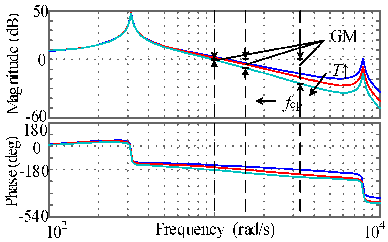
Figure 13.
Experimental platform.
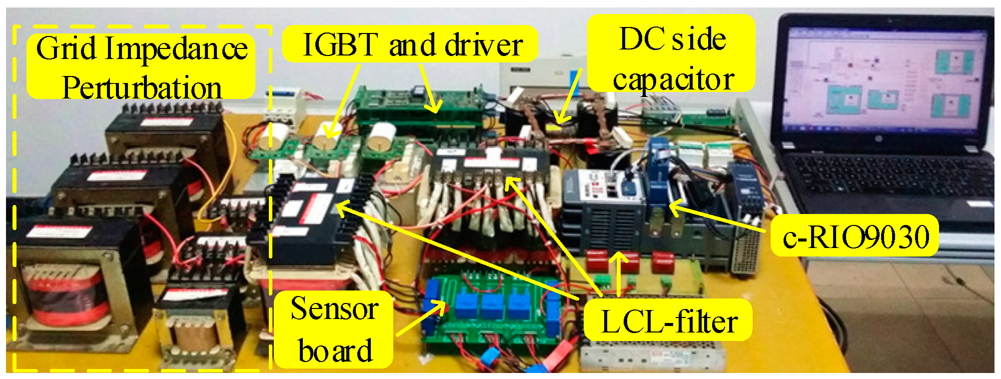
Figure 14.
Experimental results of the traditional control strategy with a quasi-PR controller of grid impedance perturbation, with Lg changing from 0 mH to 0.8 mH at t1, and Lg changing from 0.8 mH to 1.2 mH at t2. (a) Grid-side current, (b) Point of common coupling (PCC) voltage.
Figure 14.
Experimental results of the traditional control strategy with a quasi-PR controller of grid impedance perturbation, with Lg changing from 0 mH to 0.8 mH at t1, and Lg changing from 0.8 mH to 1.2 mH at t2. (a) Grid-side current, (b) Point of common coupling (PCC) voltage.
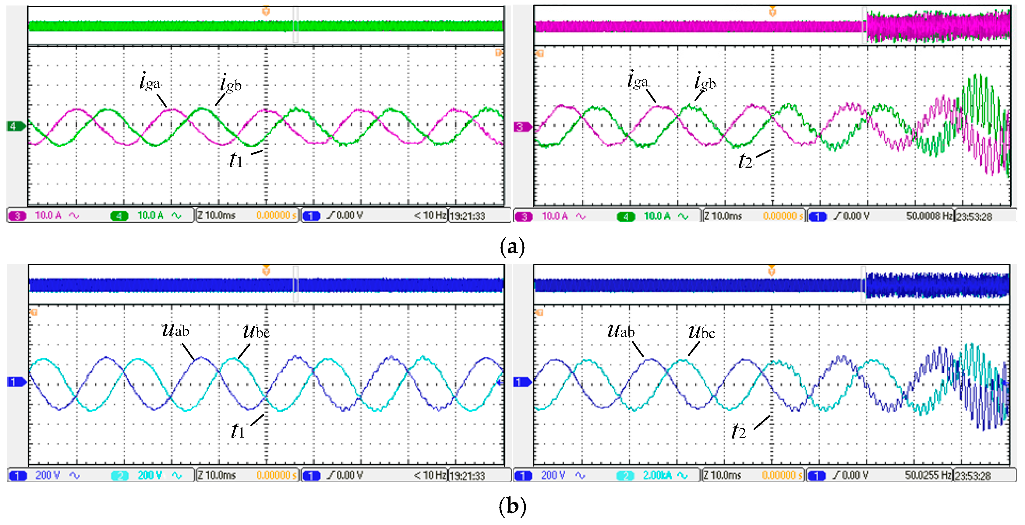
Figure 15.
The total harmonic distribution (THD) of the three-phase currents and PCC voltages under traditional control strategy with quasi-PR controller when Lg is 0 mH and 0.8 mH. (a) THD of grid-side current; (b) THD of PCC voltage.
Figure 15.
The total harmonic distribution (THD) of the three-phase currents and PCC voltages under traditional control strategy with quasi-PR controller when Lg is 0 mH and 0.8 mH. (a) THD of grid-side current; (b) THD of PCC voltage.
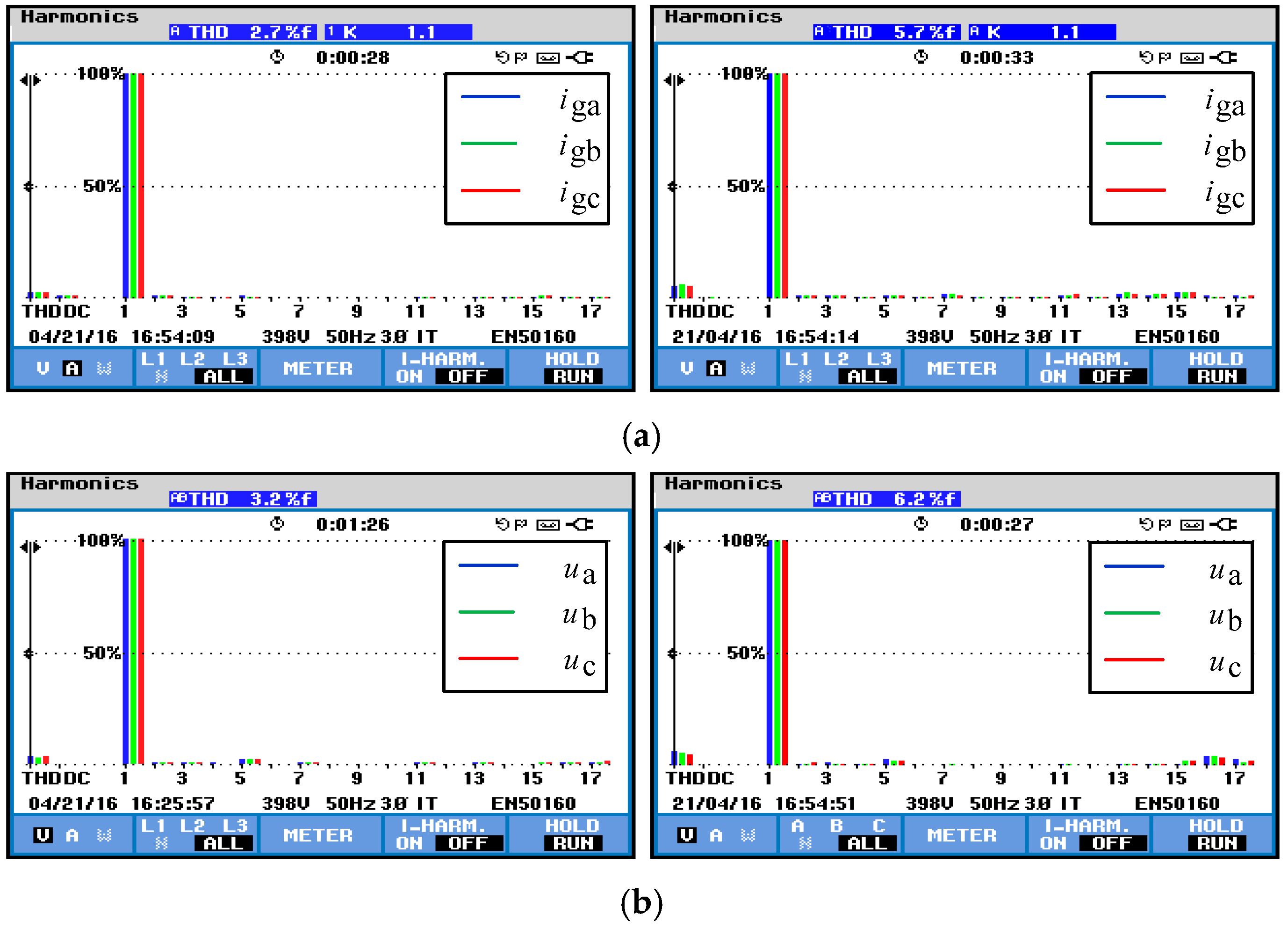
Figure 16.
Experimental results under the proposed H∞ robust control strategy on grid impedance perturbation, with Lg changing from 0 mH to 0.8 mH at t1; Lg changing from 0.8 mH to 1.2 mH at t2; and Lg changing from 1.2 mH to 4.5 mH: (a) Grid-side current, (b) PCC voltage.
Figure 16.
Experimental results under the proposed H∞ robust control strategy on grid impedance perturbation, with Lg changing from 0 mH to 0.8 mH at t1; Lg changing from 0.8 mH to 1.2 mH at t2; and Lg changing from 1.2 mH to 4.5 mH: (a) Grid-side current, (b) PCC voltage.
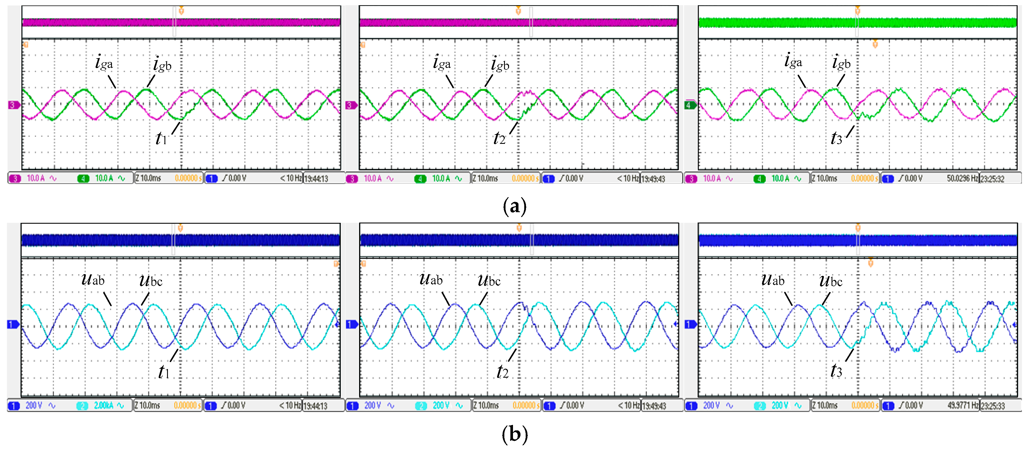
Figure 17.
THD of three-phase currents and PCC voltages under the proposed H∞ robust control strategy when Lg is 0.8 mH, 1.2 mH, and 4.5 mH. (a) THD of the grid-side current, (b) THD of PCC voltage.
Figure 17.
THD of three-phase currents and PCC voltages under the proposed H∞ robust control strategy when Lg is 0.8 mH, 1.2 mH, and 4.5 mH. (a) THD of the grid-side current, (b) THD of PCC voltage.
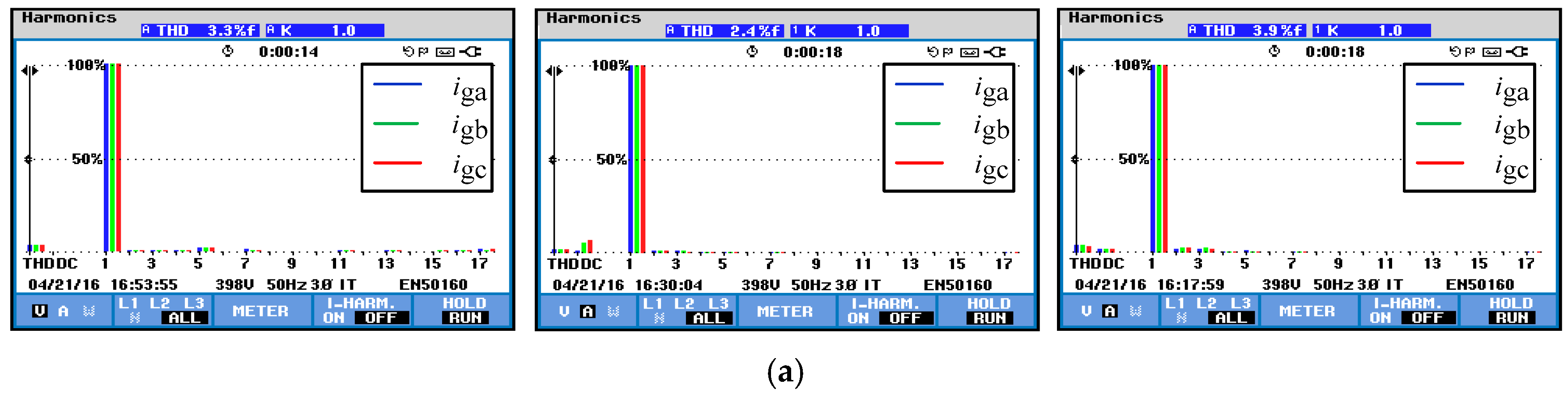
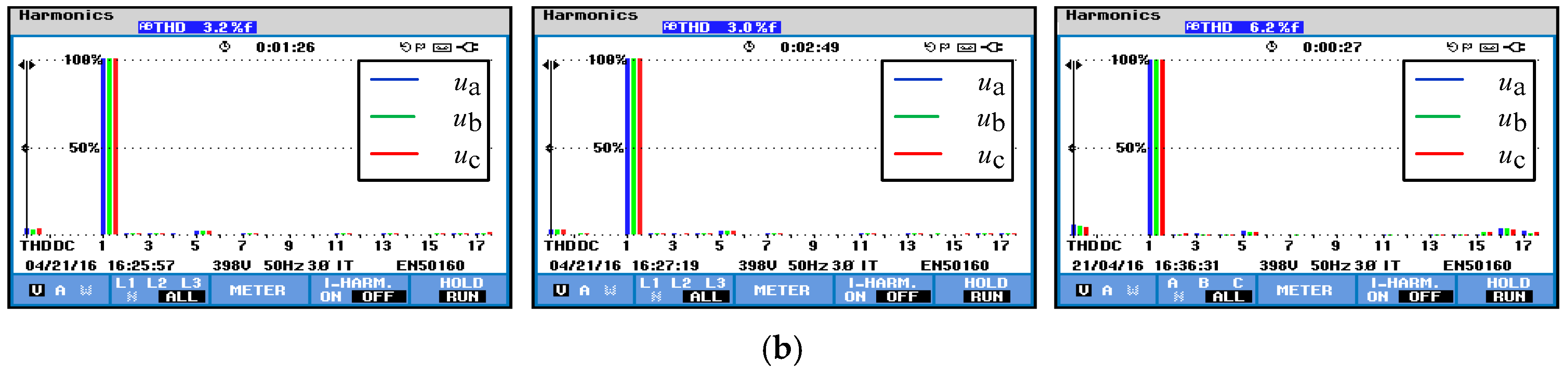
Figure 18.
Experimental waveforms under the H∞ robust control strategy when Lg is 4.5 mH: (a) Iref changing from 9 A to 11 A, (b) Grid voltage dropping from 190 V to 120 V Direct-Current (DC), (c) voltage dropping from 400 V to 330 V.
Figure 18.
Experimental waveforms under the H∞ robust control strategy when Lg is 4.5 mH: (a) Iref changing from 9 A to 11 A, (b) Grid voltage dropping from 190 V to 120 V Direct-Current (DC), (c) voltage dropping from 400 V to 330 V.


Table 1.
System parameters.
| System Parameters | ||
|---|---|---|
| Rated power | 2 kW | |
| DC voltage | 400 V | |
| Grid phase voltage | 110 V | |
| Frequency | 50 Hz | |
| Switching frequency | 5 kHz | |
| Sampling frequency | 5 kHz | |
| LCL filter | Lf1 | 2 mH |
| Lf2 | 0.5 mH | |
| Cf | 40 μF | |
| Grid impedance | Lg | [0–4.5] mH, Lgnom = 1.2 mH |
| rg | 0.1 Ω | |
© 2018 by the authors. Licensee MDPI, Basel, Switzerland. This article is an open access article distributed under the terms and conditions of the Creative Commons Attribution (CC BY) license (http://creativecommons.org/licenses/by/4.0/).
Share and Cite
MDPI and ACS Style
Wang, Y.; Wang, J.; Zeng, W.; Liu, H.; Chai, Y. H∞ Robust Control of an LCL-Type Grid-Connected Inverter with Large-Scale Grid Impedance Perturbation. Energies 2018, 11, 57. https://doi.org/10.3390/en11010057
AMA Style
Wang Y, Wang J, Zeng W, Liu H, Chai Y. H∞ Robust Control of an LCL-Type Grid-Connected Inverter with Large-Scale Grid Impedance Perturbation. Energies. 2018; 11(1):57. https://doi.org/10.3390/en11010057
Chicago/Turabian StyleWang, Yingjie, Jiashi Wang, Wei Zeng, Haiyuan Liu, and Yushuo Chai. 2018. "H∞ Robust Control of an LCL-Type Grid-Connected Inverter with Large-Scale Grid Impedance Perturbation" Energies 11, no. 1: 57. https://doi.org/10.3390/en11010057
Note that from the first issue of 2016, this journal uses article numbers instead of page numbers. See further details here.